Bose-Einstein Condensate in a Linear Trap With a Dimple Potential

Abstract

We study Bose-Einstein condensation in a linear trap with a dimple potential where we model dimple potentials by Dirac $\delta$ function. Attractive and repulsive dimple potentials are taken into account. This model allows simple, explicit numerical and analytical investigations of noninteracting gases. Thus, the Schrödinger equation is used instead of the Gross-Pitaevski equation. We calculate the atomic density, the chemical potential, the critical temperature and the condensate fraction. The role of the relative depth of the dimple potential with respect to the linear trap in large condensate formation at enhanced temperatures is clearly revealed. Moreover, we also present a semi-classical method for calculating various quantities such as entropy analytically. Moreover, we compare the results of this paper with the results of a previous paper in which the harmonic trap with a dimple potential in 1D was investigated.

1 Introduction

The experimental realization of Bose-Einstein condensates (BEC) of dilute gases of alkalis ${}^{87}Rb$, ${}^{23}Na$ and ${}^{7}Li$ were observed at very low temperatures following the improvement in cooling and trapping techniques [1, 2, 3]. A finite number of atoms $N$ which are confined in spatially inhomogeneous trapping potentials are possible experimentally. Despite the enhanced importance of phase fluctuations [4], several studies [5, 6] showed that BEC can occur in harmonically trapped lower-dimensional systems for finite $N$. Bose-Einstein condensation in one dimension (1D) with a harmonic trap is attractive due to the enhanced critical temperature and the condensate fraction [5, 6]. One- and two- dimensional BECs were created in experiments[7]. One-dimensional quasicondensates were also generated on a microchip [8, 9] and in lithium mixtures [10] a decade ago.

The possibility of using all optical power-law traps have been proposed for fast and efficient production of Bose-Einstein condensates very recently[11]. Taking into account weakly interacting Bose gases, theoretical and experimental investigation of momentum distribution of weakly interacting one-dimensional (1D) Bose gases at the quasicondensation crossover have been studied [12].

Using the semiclassical approximation, one can show that Bose-Einstein condensation in one dimensional harmonic traps are not stable[13]. Indeed, in all (1D) BEC experiments with ${}^{87}Rb$, ${}^{23}Na$ and ${}^{7}Li$, the (1D) objects resembling BEC that have been created are ”quasi-condensates”, which have suppressed density fluctuations where the phase still fluctuates along the cloud, and no single quantum state is macroscopically occupied. In all of these experiments, the phase coherence length is much smaller than the size of the cloud. The transition to the quasicondensate regime is governed by interactions. (see Ref. [14] and references therein). The conditions for having interaction induced quasicondensation versus finite-size condensation (1D BEC formation) have been studied precisely [15]. In typical experiments (and actually all cases so far), interactions are too strong to allow for the (1D) BEC instead of the quasicondensate.

Cavalcanti et.al. showed even 3D gases in the presence of a uniform field do not go undergo Bose-Einstein condensation at finite temperatures [16]. However, the authors have revealed that if there is a point-like impurity at the bottom of the vessel, Bose-Einstein condensation occurs at $T\neq 0$. Moreover, as mentioned in a previous paper, modification of the shape of the trapping potential can be used to increase the phase space density [17]. “Dimple”-type potentials are the most favorable potentials for this purpose. The phase-space density can be enhanced by an arbitrary factor by using a dimple potential at the equilibrium point of the harmonic trapping potential [18, 19]. The formation of a Bose-Einstein condensate in a cigar-shaped three-dimensional harmonic trap, induced by the controlled addition of an attractive ”dimple” potential along the $z$ axis has been realized very recently [20]. Moreover, the effect of variations of the longitudinal trap frequency on the BEC profile has been analytically treated by using delta kicks [21] and the ground state properties of 1D quantum gases in a harmonic trap in the presence of a point-like attractive potential have been also investigated [22].

A simple magnetic trap mechanism is called quadrupole trap which varies linearly in all directions and vanishes at the center. This trapping mechanism has been used to obtain BEC of dilute gases however it has a major disadvantage that there can be appreciable losses in the vicinity of the node in the field [23]. There have been attempts to overcome this disadvantage of the simple quadrupole trap [2, 23]. Dimple type potentials are good candidates for this reason. Therefore we study the properties of a BEC in a V shaped potential with a dimple at the center. Attractive and repulsive dimple potentials are taken into account. We model the dimple potential using a Dirac $\delta$ function. The delta function can be defined via a Gaussian function [24] $g(x,a)=(1/\sqrt{\pi}a)\exp{(-x^{2}/a^{2})}$ of infinitely narrow width $a$ so that $g(x,a)\rightarrow\delta(x)$ for $a\rightarrow 0$. This allows for analytical calculations in some limiting cases as well as a simpler numerical treatment for arbitrary parameters. The Schrödinger equation for a particle in the V-shaped potential decorated by a repulsive or attractive Dirac delta function interaction at the center has been solved very recently [25]. We apply this potential as a model for quadrupole trap with a dimple. We also compare the results of this paper with the results of a previous paper in which the harmonic trap with a dimple potential in 1D was investigated [18]. On one hand, the linear trap could be imagined as a disadvantageous against harmonic trap applications. However, experimental easiness of may lead experimentalists to prefer quadrupole trap with a dimple.

We calculate the transition temperature as well as the chemical potential and condensate fraction for various number of atoms and for various relative depths of the dimple potential. For describing a system with interacting particles, the Gross-Pitaevski equation is usually utilized. We note that we neglect the interactions between the atoms in our model, and thus the Schrödinger equation for the linear trap with the dimple potential is solved.

The paper is organized as follows. In Sect. II, we present the analytical solutions of the Schrödinger equation for a Dirac $\delta$-decorated linear potential and the corresponding eigenvalue equation. In Sect. III, we present a semiclassical approach and calculate the entropy of a Bose gas in a V shaped potential. In Sec. IV, determining the eigenvalues numerically, we show the effect of the dimple potential on the condensate fraction, the transition temperature and the chemical potential. Finally, we present our conclusions in Sect. V.

2 Linear confining potential decorated with a Dirac $\delta$ potential at the origin

We begin our discussion with the one dimensional linear potential decorated with a Dirac $\delta$ function at x=0, ($\delta(x)$) . This potential is given as:

$$V(x)=f|x|-\frac{\hbar^{2}}{2m}\sigma\delta(x),$$ (1)

where $m$ is the mass of the particles, $f$ is force term due to the linear trap and $\sigma$ is the strength (depth) of the dimple potential located at $x=0$. The factor $\hbar^{2}/2m$ is used for calculational convenience. The negative $\sigma$ values represent repulsive interaction while the positive $\sigma$ values represent attractive interaction. The time-independent Schrödinger equation for the potential given in Equation (1) is:

$$-\frac{\hbar^{2}}{2m}\frac{d^{2}\Psi(x)}{dx^{2}}+V(x)\Psi(x)=E\Psi(x).$$ (2)

Although the solution of this equation can be found easily we summarize it for the sake of completeness. First, we solve Equation (2) for $x\neq 0$. Since the potential is an even function, the eigenstates of this potential are even and odd functions (see e.g. [26]). Hence it is enough to find the solution for positive $x$. Defining $k^{2}=2mE/\hbar^{2}$, $l=\left(\hbar^{2}/(2mf)\right)^{1/3}$ and $u=x/l-k^{2}l^{2}$ for $x>0$ and inserting these definitions into Equation (2) one gets the Airy differential equation for the variable $u$ [27]:

$$\frac{d^{2}\Psi(u)}{du^{2}}-u\,\Psi(u)=0$$ (3)

Therefore, utilizing the fact that the wave functions are either even or odd, one finds the wave functions in terms of Airy Ai function $Ai(x)$ as [27] :

$$\Psi_{e}(x) = c^{e}_{n}\,Ai[\frac{1}{l}(|x|-k_{n}^{2}l^{3})]\quad\rm{~{}for~{}}n=0,2,\ldots$$

$$\Psi_{o}(x) = c^{o}_{n}sgn(x)Ai[\frac{1}{l}(|x|-k_{n}^{2}l^{3})]\quad\rm{~{}for~{}}n=1,3,\ldots\;.$$ (4)

for $\sigma=0$ in Equation (1). Here, $c^{e}_{n}$ and $c^{o}_{n}$ are the normalization constants for even and odd wave functions respectively and $sgn(x)$ stands for the sign function. The $c^{e}_{n}$ and $c^{o}_{n}$ can be found using the roots of $Ai(x)$ and the derivative of AiryAi function $Ai^{\prime}(x)$ [27]. Both $Ai(x)$ and $Ai^{\prime}(x)$ have infinite number of zeros and all the roots of these functions are negative. Let us denote the roots of $Ai(x)$ by $-s_{n}$ and the roots of $Ai^{\prime}(x)$ by $-z_{n}$, i.e $Ai(-s_{n})=Ai^{\prime}(-z_{n})=0$. These coefficients can be ordered as $-z_{1}<-s_{1}<-z_{2}<-s_{2}<\ldots$ . Ordering these coefficients just using one symbol like $\alpha_{0}=z_{1},\alpha_{1}=s_{1},\ldots\alpha_{2n-1}=s_{n},\alpha_{2n-2}=z_{n},\;n=1,2,\ldots$, one gets for the normalization coefficients [27]:

$$c^{e}_{n} = \left[2\alpha_{n}l\left[Ai(-\alpha_{n})\right]^{2}\right]^{-1/2}\quad\rm{~{}for~{}}n=0,2,\ldots$$

$$c^{o}_{n} = \left[2lAi^{\prime}(-\alpha_{n})\right]^{-1}\quad\rm{~{}for~{}}n=1,3,\ldots\;.$$ (5)

Using the fact that $\Psi_{o}(0)=0$ and $(d\Psi_{e}(x)/dx)_{x=0}=0$, one finds the eigenvalues of the Hamiltonian whose the potential term is given in Equation (1) for $\sigma=0$:

$$E_{n}=\left(\frac{\hbar^{2}f^{2}}{2m}\right)^{1/3}\alpha_{n}\quad\rm{for~{}}n=0,1,\ldots\;.$$ (6)

We define

$$k_{n}=\sqrt{(2mE_{n})}/\hbar.$$ (7)

Using $l=\left(\hbar^{2}/(2mf)\right)^{1/3}$ we get

$$k_{n}=\sqrt{\alpha_{n}}/l\quad\rm{for~{}}n=0,1,\ldots\;.$$ (8)

If $\sigma$ in Equation (1) is not zero, the eigenvalues of the even states can be found by taking the integral of the Schrödinger equation from $-\epsilon$ to $\epsilon$ in the limit $\epsilon\rightarrow 0$:

$$\lim_{\epsilon\to 0} \left(-\frac{\hbar^{2}}{2m}\int\limits^{\epsilon}_{-\epsilon}\frac{d^{2}\Psi(x)}{dx^{2}}dx+f\int\limits^{\epsilon}_{-\epsilon}|x|\Psi(x)dx-\frac{\hbar^{2}}{2m}\sigma\int\limits^{\epsilon}_{-\epsilon}\delta(x)\Psi(x)dx\right)=$$ (9)

$$\lim_{\epsilon\to 0} \,E\int\limits^{\epsilon}_{-\epsilon}\Psi(x)dx.$$

Since the functions $|x|\psi(x)$ and $\psi(x)$ are continuous at $x=0$ the second integral on the left hand side and the integral on the right hand side of the Equation (9) vanish. Therefore this equation reduces to

$$\lim_{\epsilon\to 0}\frac{d\psi(x)}{dx}|_{x=\epsilon}-\frac{d\psi(x)}{dx}|_{x=\epsilon}+\sigma\psi(0)=0$$ (10)

This equation reveals that the derivative of the even eigenfunctions are not continuous when $\sigma\neq 0$. Therefore, the eigenvalues of the even eigenfunctions cannot be found from the roots of $Ai^{\prime}(x)$ in this case. However, substituting $\Psi_{e}(x)$ in Equation (4) for the $\psi(x)$ into the Equation (10) we get an equation for the eigenvalues of the even eigenfunctions for the potential given in Equation (1) for $\sigma\neq 0$:

$$\frac{2Ai^{\prime}(-k_{n}^{2}l^{2})}{Ai(-k_{n}^{2}l^{2})}=-\sigma l.$$ (11)

This equation can be solved numerically for $k_{n}$. Substituting these $k_{n}$ values into the argument of AiryAi function for even wave functions in Equation (4) one gets the even eigenfunctions for $\sigma\neq 0$ of the Hamiltonian for the potential given in Equation (1).

The odd wave functions vanish at $x=0$. Hence their derivatives are continuous and they are not affected by Dirac $\delta$ function at the origin. Therefore the eigenvalues corresponding to the odd eigenfunctions of the potential in Equation (1) are the same with the eigenvalues of odd eigenfunctions of the potential $V(x)=f|x|$. On the other hand, we showed that the energy eigenvalues of even states change as a function of $\sigma$. As shown in Ref. [25], the ground state energy eigenvalue decreases without a lower limit as $\sigma$ increases (attractive case). However, the energies of the excited even states are limited by the energies $E_{2n+1}$ of odd states and as $\sigma\rightarrow\infty$, $E_{2n+2}\rightarrow E_{2n+1}$ where $n=0,1,...$.

3 Semiclassical Approach

We will first investigate Bose gas in a V shaped potential with a Dirac $\delta$ at the origin semiclassically . The spectrum of the Hamiltonian with the potential in Equation (1) is discrete for all values of $\sigma$ including $\sigma=0$ (only the linear confining potential). For convenience, we define a dimensionless parameter $\Lambda$ in terms of $\sigma$ as:

$$\Lambda=\sigma l.$$ (12)

We choose the value of $l$ such that $\Lambda$ defined in equation above has the same order of magnitude with $\Lambda$ values defined in Ref. [18] for a given $\sigma$, so that we can compare the effect of dimple potential to the linear confining potential with the effect of dimple potential to the the harmonic trap. In [18] the calculations are made for ${}^{23}Na$ particles with $m=23$ amu and the frequency $\omega$ of the harmonic trap was chosen as $\omega=2\pi 21Hz$. Equating the length scales of the harmonic trap $\sqrt{\hbar/(2m\omega)}$ to the length scale of the confining linear potential $l$, we get for $l=3.23\mu m$.

Quantum mechanically - as we will present in the following section- one calculates the thermodynamic variables of a non-interacting condensate like critical temperature, condensate fraction and the chemical potential taking sums over the discrete energy eigenvalues. However, in the semiclassical approximation one uses the density of states and employs integrals instead of sums (see e.g. [23, 28]). Therefore we first find the density of states for a linear confining potential. As we have showed in the previous section, the odd and even energy eigenvalues of the linear confining potential ($\sigma=0$ in Equation (1)) is proportional to the negative of the root values of $Ai(x)$ and to the $Ai^{\prime}(x)$ ($s_{n}$ and $z_{n}$ values defined in the previous section), respectively. This proportionality can be used to calculate the density of states for linear confining potential. The $s_{n}$ values can be approximated by the formula [27], :

$$-s_{n}\approx[\frac{3\pi}{2}(n-\frac{1}{4})]^{2/3}.$$ (13)

$-s_{n}$ values are an approximation to the roots of $Ai$. Using the definitions $\alpha_{n}$, $s_{n}$ and Equation (6), we get an equality between $s_{n}$ and the eigenenergies of odd states as $-s_{n}=(2m/\hbar^{2}f^{2})^{1/3}E_{n}$. We take $n$ and therefore $E_{n}\equiv E$ as continuous variables and get $\frac{3\pi}{2}(n-\frac{1}{4})=(2m/\hbar^{2}f^{2})^{1/2}E^{3/2}$. So we obtain the density of the odd states

$$\frac{dn}{dE}=\frac{1}{\pi}(\frac{2m}{\hbar^{2}f^{2}})^{1/2}E^{1/2}.$$ (14)

For each odd state there is an even state. Hence the density of states ($g(E)$) for the linear confining potential is

$$g(E)=\frac{2}{\pi}(\frac{2m}{\hbar^{2}f^{2}})^{1/2}E^{1/2}.$$ (15)

Using the density of states one can calculate the number of particles $N_{T}$ in the thermal gas that is the number of particles which are not in condensate phase [23]. Above the critical temperature $T_{c}$ the number of particles in the ground state is negligible and all the particles are assumed to be in the thermal gas. As the temperature decreases the chemical potential increases and comes very close to the ground state energy. Therefore one gets the critical temperature taking the chemical potential $\mu$ equal to the ground state value [28]. Using the density of states and Bose distribution we find:

$$N=\int_{\epsilon_{1}}^{\infty}\frac{g(\epsilon)}{e^{\beta_{c}(\epsilon-\mu)-1}}d\epsilon=\frac{2}{\pi}(\frac{2m}{\hbar^{2}f^{2}})^{1/2}\int_{\epsilon_{1}}^{\infty}\frac{\epsilon^{1/2}}{e^{\beta_{c}(\epsilon-\mu)-1}}d\epsilon$$ (16)

where the lower limit of the integral is the energy eigenvalue of the first excited state and $\beta_{c}=1/(k_{B}T_{c})$. For different $\Lambda$ values which are used to model the strength of the dimple potential we can find the energy eigenvalue of the ground state using Equation (11). The energy eigenvalue of the first excited state is same for all $\Lambda$ and found by Equation (6) taking $n=1$ because it is an odd eigenfunction. The Dirac $\delta$ potential in Equation (1) does not change the density of states. That is it does not create or destroy eigenstates but only change the values of the energy eigenvalues. Therefore the same density of state expression can be used for all $\Lambda$ values. However, the total number of particles in the thermal gas or (in the condensate) differ for different $\Lambda$ values because as $\Lambda$ varies the energy eigenvalue of the ground state varies which cause a change in the chemical potential value.

So, if the Equation (16) can be solved for $\beta_{c}$ for fixed N, one can find the change of critical temperature with increasing $\sigma$ which determines the strength of the dimple potential. We approximately calculate the integral in Equation (16) taking the lower limit zero (i.e we set $\epsilon_{1}=0$) and shifting the chemical potential by the same amount ($\mu\rightarrow\mu-\epsilon_{1}$). Applying these approximations we take the integral in Equation (16) and find

$$N\approx 2(\frac{2m}{\pi\hbar^{2}f^{2}})^{1/2}(\frac{1}{\beta_{c}})^{3/2}g_{3/2}(e^{\beta_{c}\mu}).$$ (17)

where the Bose function $g_{p}(x)$ is defined as [23]:

$$g_{p}(x)=\sum_{l=1}^{\infty}\frac{x^{l}}{l^{p}}\,.$$ (18)

We have solved Equation (17) and find $T_{c}$ for various $\Lambda$ values. We will present our results in the following section in order to compare the results obtained from semiclassical approximation with the results obtained from quantum mechanical calculations.

Adding a dimple potential adiabatically changes the critical temperature by changing the value of chemical potential $\mu$ [28]. If an attractive dimple is added to the trap potential at temperatures slightly above the critical temperature of the trap without a dimple adiabatically, the entropy remains constant. Hence the decrease in the ground state energy cause the formation of BEC [28]. In the laboratory this process can be maintained adiabatically and the entropy of the boson gas remains constant during the process. Therefore if one finds an expression for the entropy of the Bose gas one can calculate the value of condensate fraction of a BEC obtained for an adiabatic process.

The entropy of a non-interacting Bose gas is easily calculated using the grand potential $\Omega$ [28]:

$$\Omega=\Omega_{0}+k_{B}T\sum_{i}ln[1-e^{\beta(\mu-\epsilon_{i})}].$$ (19)

Using the density of states for a linear confining potential given in Equation (15), the grand potential of a non-interacting Bose gas trapped using linear confining potential can be written as

$$\Omega=\Omega_{0}+\frac{2k_{B}T}{\pi}(\frac{2m}{\hbar^{2}f^{2}})^{1/2}\int_{\epsilon_{1}}^{\infty}\epsilon^{1/2}\ln[1-e^{\beta(\mu-\epsilon)}]\,\rmd\epsilon.$$ (20)

Calculating the integral in Equation (20) one finds

$$\Omega=\Omega_{0}-\frac{2}{\pi}(\frac{2m}{\hbar^{2}f^{2}})^{1/2}\times$$

$$\left[\frac{\sqrt{\epsilon_{1}}}{\beta^{2}}g_{2}(e^{\beta(\mu-\epsilon_{1})})+\frac{\sqrt{\pi}}{2\beta^{5/2}}\sum_{n}^{\infty}\frac{e^{n\beta\mu}\rm{Erfc}(\sqrt{n\beta\epsilon_{1}})}{n^{5/2}}\right]$$ (21)

where $\beta=1/(k_{B}T)$, $\rm{Erfc}(x)=1-\rm{Erf}(x)=1-(2/\sqrt{\pi})\int_{0}^{x}e^{-t^{2}}dt$ and $g_{p}(x)$ is defined in (18). Then, we find the entropy by $S=-d{\Omega}/{dT}$:

$$S=k_{B}\frac{2}{\pi}(\frac{2m}{\hbar^{2}f^{2}})^{1/2}\times$$

$$\bigg{\{}\frac{5\sqrt{\epsilon_{1}}}{2\beta}g_{2}(e^{\beta(\mu-\epsilon_{1})})+\sqrt{\epsilon_{1}}(\mu-\epsilon_{1})\ln[1-e^{\beta(\mu-\epsilon_{1})}]+$$

$$\frac{5\sqrt{\pi}}{2\beta^{3/2}}\sum_{n=1}^{\infty}(\frac{e^{n\beta\mu}\rm{Erfc}(\sqrt{n\beta\epsilon_{1}})}{n^{5/2}})-\frac{\sqrt{\pi}\mu}{2\beta^{1/2}}\sum_{n=1}^{\infty}\frac{e^{n\beta\mu}\rm{Erfc}(\sqrt{n\beta\epsilon_{1}})}{n^{3/2}}\bigg{\}}.$$

(22)

For the temperatures slightly above $T_{c}$, one can take $\mu=\epsilon_{0}$ and $\beta=\beta_{c}$. Therefore for temperatures slightly above $T_{c}$, Equation(22) becomes

$$S=k_{B}\frac{2}{\pi}(\frac{2m}{\hbar^{2}f^{2}})^{1/2}\times$$

$$\bigg{\{}\frac{5\sqrt{\epsilon_{1}}}{2\beta_{c}}g_{2}(e^{\beta_{c}(\epsilon_{0}-\epsilon_{1})})+\sqrt{\epsilon_{1}}(\epsilon_{0}-\epsilon_{1})\ln[1-e^{\beta_{c}(\epsilon_{0}-\epsilon_{1})}]$$

$$+\frac{5\sqrt{\pi}}{2\beta_{c}^{3/2}}\sum_{n=1}^{\infty}(\frac{e^{n\beta_{c}\epsilon_{0}}\rm{Erfc}(\sqrt{n\beta_{c}\epsilon_{1}})}{n^{5/2}})$$

$$-\frac{\sqrt{\pi}\epsilon_{0}}{2\beta_{c}{1/2}}\sum_{n=1}^{\infty}\frac{e^{n\beta_{c}\epsilon_{0}}\rm{Erfc}(\sqrt{n\beta_{c}\epsilon_{1}})}{n^{3/2}}\bigg{\}}$$

(23)

where $\epsilon_{0}=\left(\frac{\hbar^{2}f^{2}}{2m})^{1/3}\right)z_{1}$ and $\epsilon_{1}=\left(\frac{\hbar^{2}f^{2}}{2m})^{1/3}\right)s_{1}$. Adding a dimple potential changes the ground state therefore the chemical potential changes also because $\mu=\epsilon_{g}<\epsilon_{0}$. So, we get

$$S=k_{B}\frac{2}{\pi}(\frac{2m}{\hbar^{2}f^{2}})^{1/2}\times$$

$$\bigg{\{}\frac{5\sqrt{\epsilon_{1}}}{2\beta}g_{2}(e^{\beta_{f}(\epsilon_{g}-\epsilon_{1})})+\sqrt{\epsilon_{1}}(\epsilon_{g}-\epsilon_{1})\ln[1-e^{\beta_{f}(\mu-\epsilon_{1})}]$$

$$+\frac{5\sqrt{\pi}}{2\beta_{f}^{3/2}}\sum_{n=1}^{\infty}(\frac{e^{n\beta_{f}\epsilon_{g}}\rm{Erfc}(\sqrt{n\beta_{f}\epsilon_{1}})}{n^{5/2}})$$

$$-\frac{\sqrt{\pi}\epsilon_{0}}{2\beta_{f}{1/2}}\sum_{n}^{\infty}\frac{e^{n\beta_{f}\epsilon_{g}}\rm{Erfc}(\sqrt{n\beta_{f}\epsilon_{1}})}{n^{3/2}}\bigg{\}}.$$

(24)

for the entropy of the BEC in the linear trap with a dimple potential where $\beta_{f}=1/(k_{b}T_{f})$ and $T_{f}$ is the final temperature of the system. Since we model the dimple potential with a Dirac $\delta$ potential, we can calculate the new ground state energy ($\epsilon_{g}$), -i.e the ground state energy of the trap with a dimple- using Equation (11). Then, we equate Equation (23) and Equation (24) to calculate the final temperature of the system, because the entropy remains constant during adiabatic process. Then, we calculate condensate fraction for this final temperature.

We present the increase of the condensate fraction with the decrease in the ground state energy value in Fig. (1). To obtain this figure, we have first calculated the ground state energy values ($\epsilon_{g}$’s) of linear confining potential with a dimple potential for different strengths of the dimple i.e for different $\sigma$ ($\Lambda$) values in our model. Then applying the procedure outlined in the previous paragraph we find $T_{f}$. Finally, we use Equation (17) to find the number of particles in the thermal gas $N_{T}$. Since we assume that the number of particles $N$ in the Bose gas is fixed we get the condensate fraction using ($N_{0}/N=1-N_{T}/N$). We choose the range of $\sigma$ values which determines the strength of the dimple same as in the paper [18], i.e. between $0\,\mathrm{m}^{-1}$ and $10^{8}\,\mathrm{m}^{-1}$.

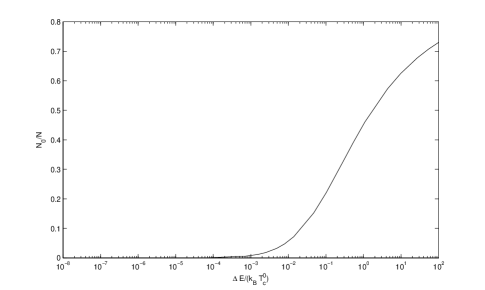
Figure 1: The condensate fraction values evaluated with the semiclassical method for $N=10^{4}$. The logarithmic scale is used for x axis, where $\Delta E=\epsilon_{0}-\epsilon_{g}$.

4 BEC In a One-Dimensional Linear Potential with a Dirac $\delta$ Function

In this section, we will investigate the behavior of a BEC confined in a one-dimensional linear confining potential decorated with a Dirac $\delta$ function given in Equation (2) quantum mechanically. That is we will use the discrete energy eigenvalues calculated numerically by Equation (8) and Equation (11) for odd ($n=1,3,\cdots$) and even ($n=0,2,\cdots$) states, respectively.

First we will investigate the change of the critical temperature as a function of $\Lambda$ which shows the effect of the dimple potential in our model.

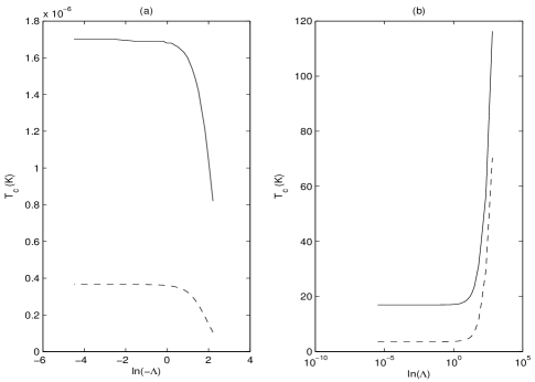
Figure 2: (a) The critical temperature $T_{c}$ vs. $\Lambda$ for $N=10^{4}$ and $N=10^{5}$ and for negative $\Lambda$. $\Lambda$ is a dimensionless variable defined in Equation (12). The solid line and the dashed line show $T_{c}$ values with decraeasing $\Lambda$ for $N=10^{4}$ and $N=10^{5}$, respectively. Here we use m $=23$ amu (${}^{23}\mathrm{Na}$) and $l=3.23\mu m$. The logarithmic scale is used for $-\Lambda$ axis. (b) The critical temperature $T_{c}$ vs. $\Lambda$ for $N=10^{4}$ and $N=10^{5}$ and for positive$\Lambda$. The logarithmic scale is used for $\Lambda$ axis.

We will present the change of the critical temperature with respect to $\Lambda$ both for attractive and repulsive dimple. The critical temperature ($T_{c}$) is obtained by taking the chemical potential equal to the ground state energy ($\mu=E_{g}=E_{0}$) and

$$N\approx\sum_{i=1}^{\infty}\frac{1}{e^{\beta_{c}\varepsilon_{i}}-1}\;\;,$$ (25)

at $T=T_{c}$, where $\beta_{c}=1/(k_{B}T_{c})$. For finite $N$ values, we define $T_{c}^{0}$ as the solution of Equation (25) for $\Lambda=0$ i.e. only for the linear confining potential.

In Equation (25), $\varepsilon_{i}$’s are the eigenvalues for the potential given in Equation (1). For $\Lambda\neq 0$ the energies of odd states are unchanged and equal to $\sqrt{\alpha_{n}}/l$ for $n=1,2,3$. The energies of even states are found by solving Equation (11) numerically. Then, these values are substituted into Equation (25); and finally this equation is solved numerically to find $T_{c}$.

For positive $\Lambda$, we present the change of $T_{c}$ with increasing $\Lambda$ for $N=10^{4}$ and $N=10^{5}$ in Fig. (2-b). For negative $\Lambda$, we present the change with increasing absolute $\Lambda$ in Figure (2-a). In this figure, logarithmic scale is used for $|\Lambda|$ axes. As $|\Lambda|$ increases, the critical temperature increases (decreases) very rapidly when $|\Lambda|\sim 10^{2}$ for positive (negative) $|\Lambda|$. However the decrease of critical temperature for negative $\Lambda$ is not as rapid as the increase for positive $\Lambda$. This is due to the fact that as $|\Lambda|$ increases for the attractive case the ground state energy value decreases indefinitely however the excited states are bounded. The limit value of the eigenenergies of the excited states with a tough dimple (modeled by a Dirac $\delta$) are the eigenvalues of the one lower level of the confining potential without a dimple. On the other hand for the repulsive case (negative $\Lambda$ in our case) all the energies with a tough dimple are bounded above by the eigenvalues of one higher level of the confining potential without a dimple.

Figure 3: The critical temperature $T_{c}$ vs. $\Lambda$ for $N=10^{4}$ for harmonic and linear trap with a dimple, respectively. $\Lambda$ is defined in Equation (12). The solid line and the dashed line show $T_{c}$ values with increasing $\Lambda$ for harmonic and linear traps, respectively. The other parameters are same as Fig. (2) The logarithmic scale is used for $\Lambda$ axis.

At this point it may be useful to compare the critical temperature values of a harmonic trap and linear trap with in 1D with the increasing depth of dimple ($\Lambda$ values in our model) . We show the change of the critical temperature with respect to $\Lambda$ for both cases in Fig. (3). The critical temperature values are higher for harmonic trap compared to linear trap if one chooses the length scales same for both potential. This is an expected result because the confinement strength of harmonic potential which increases quadratically with respect to distance to the center of the potential is larger than linear trap which increases linearly with respect to distance to the center.

As we mentioned in the previous section the increase of the critical temperature can be calculated approximately by solving Equation (16) obtained by the semi-classical method. We compare the critical temperature values obtained quantum mechanically and semiclassically in Figure (4). This figure shows that the agreement of the results of two methods is better for large $\Lambda$ (or large $\Delta E$) values. This is due to the fact that the average occupations for excited states is so low ($n^{excited}\ll 1$) that the semiclassical treatment for this gas is valid. Therefore, the semiclassical method may be useful for calculations with large $\Lambda$ values because for $\Lambda\approx 10^{3}$ the numerical calculations do not give accurate results.

Figure 4: ($T_{c}^{SC},\,T_{c})$ vs. $\Lambda$ for $N=10^{4}$. The dashed line shows the $T_{c}^{SC}$ values obtained semiclassically where the solid line shows the $T_{c}$ values obtained quantum mechanically. The logarithmic scale is used for $\Lambda$ axis.

For a gas of N identical bosons, the chemical potential $\mu$ is obtained by solving equation

$$N=\sum_{i=0}^{\infty}\frac{1}{e^{\beta(\varepsilon_{i}-\mu)}-1}=N_{0}+\sum_{i=1}^{\infty}\frac{1}{e^{\beta(\varepsilon_{i}-\mu)}-1},$$ (26)

at constant temperature and for given N, where $\varepsilon_{i}$ is the energy of state $i$. We present the change of $\mu$ as a function of $T/T_{c}^{0}$ for $N=10^{4}$ in Fig.(5) and in Fig.(6) for $\Lambda=0$ and $\Lambda=32$, respectively.

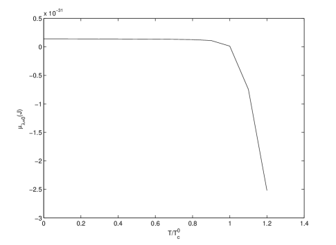
Figure 5: The chemical potential $\mu$ vs temperature $T/T_{c}^{0}$ for $N=10^{4}$ and $\Lambda=0$. The other parameters are the same as Fig. 2.

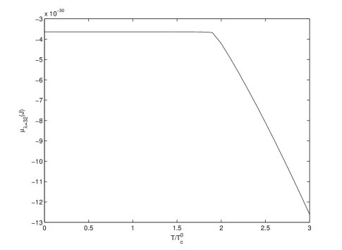
Figure 6: The chemical potential $\mu$ vs temperature $T/T_{c}^{0}$ for $N=10^{4}$ and $\Lambda=32$. The other parameters are the same as Fig. 2.

By inserting $\mu$ values into the equation

$$N_{0}=\frac{1}{e^{\beta(\varepsilon_{0}-\mu)}-1},$$ (27)

we find the average number of particle in the ground state. $N_{0}/N$ versus $T/T_{c}^{0}$ for $N=10^{4}$, $\Lambda=0,3.2,32$ are shown in Fig. (7).

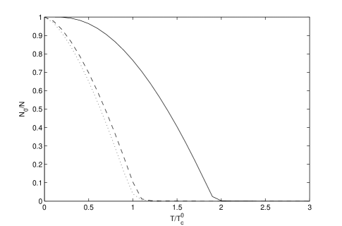
Figure 7: $N_{0}/N$ vs $T/T_{c}^{0}$ for $N=10^{4}$ dotted line for $\Lambda=0$, dashed line for $\Lambda=3.2$, solid line for $\Lambda=32$. The other parameters are the same as Fig. 2.

We also present the change of condensate fraction for $N=10^{4}$ and $N=10^{5}$ with increasing temperature for fixed $\Lambda=32$ in Fig. (8). The condensate fractions for different N values are drawn by using their corresponding $T_{c}^{0}$ values. The $T_{c}^{0}$ values are $0.37\,\mu$K for $N=10^{4}$, and $1.7\,\mu$K for $N=10^{5}$.

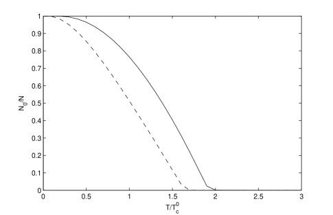
Figure 8: Condensate fraction $N_{0}/N$ vs $T/T_{c}^{0}$ for fixed $\Lambda=32$. The solid and dashed lines show condensate fraction for $N=10^{4}$ and $N=10^{5}$, respectively. Logarithmic scale is used for $\Lambda$ axis. The other parameters are the same as Fig. 2.

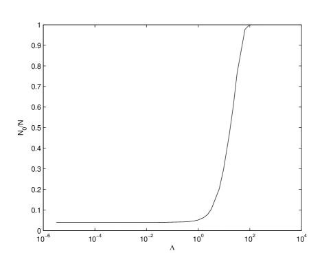
Figure 9: Condensate fraction $N_{0}/N$ vs the strength of the Dirac $\delta$ potential $\Lambda$ for $N=10^{4}$ at $T=T_{c}^{0}$. The logarithmic scale is used for $\Lambda$ axis. The other parameters are the same as Fig. 2.

We also find the condensate fraction as a function of $\Lambda$ at a constant $T=T_{c}^{0}$. These results for $N=10^{4}$ are shown in Fig. (9). We notice that large $\Lambda$ values ($\Lambda>1$) induce sharp increase in condensate fraction like in the harmonic trap with a dimple potential [18].

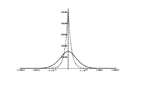
Figure 10: Comparison of density profiles of a BEC in a harmonic trap with a BEC in a harmonic trap decorated with a delta function ($\Lambda=4.6$). The solid curve is the density profile of the BEC in decorated potential. The dashed curve is the density profile of the 1D harmonic trap ($\Lambda=0$). The parameter z is dimensionless length defined after Equation (2). The other parameters are the same as Fig. 2.

Finally, we compare density profiles of condensates for a linear trap and a linear trap decorated with a delta function ($\Lambda=4.6$) in Fig. (10). Since the ground state wave functions can be calculated analytically for both cases, we find the density profiles by taking the absolute square of the ground state wave functions.

5 Conclusion

We have investigated the effect of the tight dimple potential on the linearly confined one dimensional BEC. We model the dimple potential with the Dirac $\delta$ function. In our model system, the increase in the strength of the Dirac $\delta$ function can be interpreted as increasing the depth of a dimple potential. This allows for analytical expressions for the eigenfunctions of the system and a simple eigenvalue equation greatly simplifying numerical treatment. We have calculated the critical temperature, the chemical potential and the condensate fraction and demonstrated the effect of the dimple potential. We have found that the critical temperature can be enhanced by an order of magnitude for experimentally accessible dimple potential parameters. In general, we find that $T_{c}$ increases with the relative strength for an attractive dimple and decreases for repulsive dimple for a non-interacting gas. However as our results show the decrease of the critical temperature for the negative dimple is not as rapid as the increase for the repulsive case. These results may be used to propose that the dimple potentials can be a good candidate to circumvent the disadvantage of the simple quadrupole trap mentioned in Reference [23]. Repulsive dimple can be used to repel atoms from the vicinity of the node ($x=0$) of the quadrupole trap. Moreover, it may be also possible to use attractive dimple potentials for the same reason because only dimple type potentials are also able to trap several atoms [29]. So they can prevent loosing atoms in the vicinity of the node. Moreover the increase of the critical temperature will be a further advantage for attractive dimple potentials.

We have also analyzed the change of the condensate fraction with respect to the strength of the Dirac $\delta$ function at a constant temperature ($T=T_{c}^{0}$), and with respect to temperature at a constant strength. It has been shown that the condensate fraction can be increased considerably and large condensates can be achieved at higher temperatures due to the strong localization effect of the dimple potential. Finally, we have determined and compared the density profiles of the linear trap and the decorated trap with the Dirac $\delta$ function at the equilibrium point using analytical solutions of the model system. Comparing the graphics of density profiles, we see that a dimple potential maintain a considerably higher density at the center of the linear trap.

The comparison of the critical temperature values for BEC’ s in linear trap with a dimple and harmonic potential with a dimple shows that the critical temperature values are higher for harmonic trap for the same dimple strength which is an expected result since the confinement of harmonic potential are more powerful. However the simplicity of the linear trap may still be useful in obtaining BEC.

We have also presented a semi-classical method for calculating various quantities such as entropy, critical temperature and condensate fraction. The results show that as the dimple strength increases the semi-classical approximation gives better results for non-interacting gas.

We believe that the presented results obtained for the noninteracting condensate in a quadrupole trap with a dimple by modeling dimple potentials by using a $\delta$ function can provide a theoretical model for such experiments.

References

References

- [1] M. H. Anderson, J. R. Ensher, M. R. Matthews, C. E. Wieman and E. A. Cornell Science 269 (1995) 198.
- [2] K. B. Davis, M. O. Mewes, M. R. Andrews, N. J. Van Druten, D. S. Durfee, D. M. Kurn and W. Ketterle Phys. Rev. Lett.75 (1995) 3969.
- [3] C. C. Bradley, C. A. Sackett, J. J. Tollett and R. G. Hulet Phys. Rev. Lett.75 (1995) 1687.
- [4] U. Al Khawaja, J. O. Andersen, N. P. Proukakis and H. T. C. Stoof Phys. Rev. A 66 (2002) 013615.
- [5] W. Ketterle and N. J. Van Druten Phys. Rev. A 54 (1996) 656.
- [6] N. J. Van Druten and W. Ketterle Phys. Rev. Lett.79 (1997) 549.
- [7] A. Görlitz, J. M. Vogels, A. E. Leanhardt, C. Raman, T. L. Gustavson, J. R. Abo-Shaeer, A. P. v, Gupta S, S. Inouye, T. Rosenband and W. Ketterle Phys. Rev. Lett.87 (2001) 130402.
- [8] H. Ott, J. Fortagh, G. Schlotterbeck, A. Grossmann and C. Zimmermann Phys. Rev. Lett.87 (2001) 230401.
- [9] W. Hänsel, P. Hommelhoff, T. W. Hansch and J. Reichel Nature 413 (2001) 501.
- [10] F. Schreck, L. Khaykovich, K. L. Corwin, G. Ferrari, T. Bourdel, J. Cubizolles and C. Salomon Phys. Rev. Lett.87 (2001) 080403.
- [11] G. D. Bruce, S. L. Bromley, G. Smirne, L. Torralbo-Campo, and D. Cassetari Phys. Rev. A 84 (2011) 053410.
- [12] T. Jacqmin, B. Fang, T. Berrada, T. Roscilde, and I. Bouchoule Phys. Rev. A 86 (2012) 043626.
- [13] V. I. Yukalov Phys. Rev. A 72 (2005) 033608.
- [14] J. Armijo, T. Jacqmin, K. Kheruntsyan, and I. Bouchoule Phys. Rev. A 83 (2011) 021605.
- [15] I. Bouchoule, K. Kheruntsyan, and G. V. Shlyapnikov Phys. Rev. A 75 (2007) 031606(R).
- [16] R. M. Cavalcanti, P. Giacconi, G. Pupillo and R. Soldati Phys. Rev. A 65 (2002) 053606.
- [17] P. W. H. Pinkse, A. Mosk, M. Weidemüller, M. W. Reynolds, T. W. Hijmans and J. T. M. Walraven Phys. Rev. Lett.78 (1997) 990.
- [18] H. Uncu, D. Tarhan, E. Demiralp and O. E. Mustecaplioglu Phys. Rev. A 76 (2007) 013618.
- [19] D. M. Stamper-Kurn, H.J. Miesner, A. P. Chikkatur, S. Inouye, J. Stenger and W. Ketterle Phys. Rev. Lett.81 (1998) 2194.
- [20] M. C. Garrett et all. Phys. Rev. A 83 (2011) 013630.
- [21] S. Ranjani, U. Roy, P. K. Panigrahi and A. K. Kapoor J. Phys. B: At. Mol. Opt. Phys. 41 (2008) 235301.
- [22] J. Goold, D. Donoghue and T. Busch J. Phys. B: At. Mol. Opt. Phys. 41 (2008) 215301.
- [23] C. J. Petchick and H. Smith Bose-Einstein Condensation in Dilute Gases (Cambridge University Press, Cambridge) (2001).
- [24] M. J. Lighthill An introduction to Fourier analysis and generalized functions (Cambridge: University Press) (1959).
- [25] WANG Xin, TANG Liang-Hui, WU Reng-Lai, WANG Nan, WANG Nan, LIU Quan-Hui Commun. Theor. Phys 53 (2010) 247.
- [26] L. D. Landau and E. M. Lifshitz Quantum Mechanics (Oxford: Buuterworth Heinemann) (1977).
- [27] J. Schwinger Quantum Mechanics (Berlin: Springer Verlag) (2001).
- [28] L. Pitaevskii, S. Stringari Bose-Einstein Condensation (Oxford: Clarendon Press) (2003).
- [29] Z. H. Ma, J. F. Christopher and Z. L. Cornish J. Phys. B: At. Mol. Phys.37 (2004) 3187.