Superluminal Pulse Propagation in a One-sided Nanomechanical Cavity System

Abstract

We investigate the propagation of a pulse field in an optomechanical system. We examine the question of advance of the pulse under the conditions of electromagnetically induced transparency in the mechanical system contained in a high quality cavity. We show that the group delay can be controlled by the power of the coupling field. The time delay is negative which corresponds to superluminal light when there is a strong coupling between the nano-oscillator and the cavity.

I Introduction

The experimental accomplishment of ultraslow light slowlight-exp1 in ultracold atoms by using electromagnetically induced transparencyeit1 (EIT), inspired appealing applications slowlight-apps1 ; slowlight-apps2 ; slowlight-apps3 ; slowlight-apps4 . Besides the ultraslow light, fast light effects ($v_{g}>c\,\,or\,\,v_{g}\,\,$ is negative) were observed experimentally by using a gain-assisted linear anomalous dispersion medium kuzmich ; kuzmich1 and coherent population oscillations bigelow . Slow light has been also observed in nanomechanical systems very recently painter . In this experiment, the transmitted signal delay can be tuned with control beam power in a side-coupled cavity system. There has been great interest in nanomechanical optical systems more recently painter1 ; favero ; schliesser ; aspel ; meystre ; kippenberg ; nunnenkamp ; schwab ; agarwal1 . At the same time light storage in an optical waveguide coupled to an optomechanical crystal array has been suggested that information is coherently transferred to mechanical vibrations of the array painter1 . On the other hand, quite recently optomechanical analogy of EIT in a high-quality cavity with nanomechanical mirror has been considered independently agarwal1 . The experimental analogue of electromagnetically induced transparency has been demonstrated in a room temperature cavity optomechanics setup formed by a thin semitransparent membrane within a Fabry-Perot cavity vitali1 and detailed experimental studies on optomechanical light storage in a silica microresonator have been done very recently fiore ; fiore1 . And also EIT in a cavity optomechanical system with an atomic medium has been studied zhou . Furthermore, tunable group delay of the pulse in a cavity optomechanical system with a Bose-Einstein condensate kadizhu and in a nanomechanical resonator-superconducting microwave cavity systems kadizhu1 have been studied theoretically very recently. Moreover, nonclassical states in optomechanical systems can be generated experimentally. Entangled states can be prepared between the probe light field and the oscillating nano-mirror (see Ref.marquardt and references therein). It has shown experimentally that entanglement between an optical cavity field mode and a macroscopic vibrating mirror can be generated by means of radiation pressure vitali . A theoretical work has shown that squeezing of the movable mirror can be achieved by the injection of squeezed vacuum light and a laser recently sumei .

In this work, we investigate the time delay of the weak probe field at the probe resonance in a high quality cavity nanomechanical mirror under the action of coupling laser. We investigate the propagation of a pulse field in an optomechanical system and examine the question of advance of the pulse under the conditions of electromagnetically induced transparency in the mechanical system contained in a high quality cavity. We show that the group delay can be controlled by the power of the coupling field. Before this work, there were some theoretical studies on the tunable group delay of the pulse in a cavity optomechanical system with a Bose-Einstein condensate kadizhu and in a nanomechanical resonator-superconducting microwave cavity systems kadizhu1 . However our group delay results are in disagreement with a theoretical study kadizhu1 for the nanomechanical resonator-superconducting microwave cavity systems.

II Model System

Let us consider the same model in Ref. (agarwal1 ). The pump-probe response of a nanomechanical oscillator of frequency $\omega_{m}$ is coupled to a high quality cavity via radiation pressure effects agarwal1 . As shown in Fig.(1) the system is driven by a coupling field of frequency $\omega_{c}$ and the probe field has frequency $\omega_{p}$.

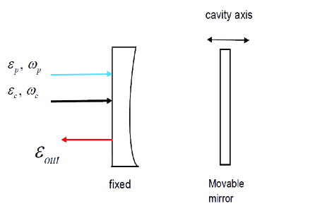
Figure 1: (Color online) Schematic of a optomechanical system coupled to a high quality cavity via radiation pressure effects adapted from Ref.agarwal1 .

The Hamiltonian of this system is agarwal1 :

$$H = \hbar\omega_{0}c^{\dagger}c+(\frac{p^{2}}{2m}+\frac{1}{2}m\omega_{m}^{2}q^{2})+i\hbar(c^{\dagger}\varepsilon_{c}e^{-i\omega_{c}t}-c\varepsilon_{c}^{\star}e^{i\omega_{c}t})$$ (1)

$$- i\hbar(c^{\dagger}\varepsilon_{p}e^{-i\omega_{p}t}-c\varepsilon_{p}^{\star}e^{i\omega_{p}t})-\chi_{0}c^{\dagger}cq,$$

where $\hat{c}^{\dagger}$ and $\hat{c}$ are the creation and annihilation operators in the cavity respectively; $p$ and $q$ are the momentum and position operators of the nanomechanical oscillator respectively; the amplitudes of the pump and probe field are introduced by $|\varepsilon_{c}|=\sqrt{2\kappa P_{c}/\hbar\omega_{c}}$ and $|\varepsilon_{p}|=\sqrt{2\kappa P_{p}/\hbar\omega_{p}}$ respectively. $P_{c}$ and $P_{p}$ are the pump and probe powers respectively. $\chi_{0}=\hbar\omega_{0}/L$ is the coupling constant between the cavity field and the movable mirror, where $L$ is the cavity length. Quantum fluctuations are not taken into account because we are dealing with the main response of the system. We use the mean field assumption $\langle Qc\rangle=\langle Q\rangle\langle c\rangle$ in order to derive Eq.(II) agarwal2 . The mean value equations are found by Heisenberg equation of motion($\langle\dot{O}\rangle=\langle 1/i\hbar[O,H]\rangle$)by adding the damping and the noise terms agarwal1 :

$$\langle\dot{q}\rangle = \frac{\langle p\rangle}{m}$$

$$\langle\dot{p}\rangle = -m\omega_{m}^{2}\langle q\rangle+\chi_{0}\langle\hat{c}^{\dagger}\rangle\langle\hat{c}\rangle-\gamma_{m}\langle p\rangle$$

$$\langle\dot{\tilde{c}}\rangle= - [\kappa+i(\omega_{0}-\omega_{c}-\frac{\chi_{0}}{\hbar}\langle q\rangle)]\langle\tilde{c}\rangle.$$

$$+ \varepsilon_{c}+\varepsilon_{p}e^{-i(\omega_{p}-\omega_{c})t}$$

At the rotating frame at the frequency $\omega_{c}$ transformed operator $\langle\tilde{c}(t)\rangle=\langle c(t)\rangle e^{i\omega_{c}t}$. If we use input-output relations collet , we obtain

$$\frac{1}{\sqrt{2\kappa}}\{\varepsilon_{out}(t)+\varepsilon_{p}e^{-i\omega_{p}t}+\varepsilon_{c}e^{-i\omega_{c}t}\}=\sqrt{2\kappa}\langle c\rangle.$$ (3)

In this system for the cavity decay rate $2\kappa$ is used. We use the following anzatsboyd in terms of probe field so as to solve Eq.(II):

$$q(t) = q_{0}+q_{+}\varepsilon_{p}e^{-i\delta t}+q_{-}\varepsilon_{p}^{*}e^{i\delta t}$$

$$p(t) = p_{0}+p_{+}\varepsilon_{p}e^{-i\delta t}+p_{-}\varepsilon_{p}^{*}e^{i\delta t}.$$ (4)

$$\tilde{c}(t) = \tilde{c}_{0}+\tilde{c}_{+}\varepsilon_{p}e^{-i\delta t}+\tilde{c}_{-}\varepsilon_{p}^{*}e^{i\delta t}$$

The field $\varepsilon_{p}$ with frequency $\omega_{p}$ is much weaker than the pump field $\varepsilon_{c}$. We obtain the steady state and first order solutions. The zeroth order and first order equations according to $\varepsilon_{p}$ are:

$$p_{0}=0$$

$$-i(\omega_{p}-\omega_{c})q_{+}=\frac{p_{+}}{m}$$ (5)

$$i(\omega_{p}-\omega_{c})q_{-}=\frac{p_{-}}{m}$$

$$-m\omega_{m}^{2}q_{0}+\chi_{0}|\tilde{c}_{0}|^{2}-\gamma_{m}p_{0}=0$$

$$-i(\omega_{p}-\omega_{c})p_{+}=-m\omega_{m}^{2}q_{+}+\chi_{0}(\tilde{c}_{0}^{\star}\tilde{c}_{+}+\tilde{c}_{0}\tilde{c}_{-}^{\star})$$ (6)

$$i(\omega_{p}-\omega_{c})p_{-}=-m\omega_{m}^{2}q_{-}+\chi_{0}(\tilde{c}_{0}^{\star}\tilde{c}_{-}+\tilde{c}_{+}^{\star}\tilde{c}_{0}).$$

$$-[\kappa+i(\omega_{0}-\omega_{c})]\tilde{c}_{0}+i\frac{\chi_{0}}{\hbar}q_{0}\tilde{c}_{0}+\varepsilon_{c}=0$$

$$-i(\omega_{p}-\omega_{c})\tilde{c}_{+}=-[\kappa+i(\omega_{0}-\omega_{c})]\tilde{c}_{+}+i\frac{\chi_{0}}{\hbar}(q_{0}\tilde{c}_{+}+q_{+}\tilde{c}_{0})+1$$ (7)

$$i(\omega_{p}-\omega_{c})\tilde{c}_{-}=-[\kappa+i(\omega_{0}-\omega_{c})]\tilde{c}_{-}+i\frac{\chi_{0}}{\hbar}(q_{0}\tilde{c}_{-}+q_{-}\tilde{c}_{0}).$$

When we use steady state equations in Eq.(II), Eq.(II), and Eq.(II), we get the steady state solutions $\langle\tilde{c}_{0}\rangle=\varepsilon_{c}/(\kappa+i\Delta)$, $\langle q_{0}\rangle=\chi_{0}|\varepsilon_{c}|^{2}/[m\omega_{m}^{2}(\kappa^{2}+\Delta^{2})]$, and $\Delta=\omega_{0}-\omega_{c}-\chi_{0}\,\,q_{0}/\hbar$. If we use first order equations in Eq.(II), Eq.(II), and Eq.(II), we get the $\tilde{c}_{+}$

$$\tilde{c}_{+}=\frac{m(\delta^{2}-\omega_{m}^{2}+i\gamma_{m}\delta)[\kappa-i(\Delta+\delta)]-i\alpha}{m(\delta^{2}-\omega_{m}^{2}+i\gamma_{m}\delta)[\kappa+i(\Delta-\delta)][\kappa-i(\Delta+\delta)]+2\Delta\alpha}$$ (8)

where $\delta=\omega_{p}-\omega_{c}$, and $\alpha=\chi_{0}^{2}|\tilde{c}_{0}|^{2}/\hbar$ .

III Results and Discussions

We can write the output field $\varepsilon_{out}(t)=\varepsilon_{out0}+\varepsilon_{out+}\varepsilon_{p}e^{-i\delta t}+\varepsilon_{out-}\varepsilon_{p}e^{i\delta t}$ boyd . Inserting this to the input-output relation and compare the first order according to the $\varepsilon_{p}$, we will get $(\varepsilon_{out+}+1)=2\kappa\tilde{c}_{+}$. $2\kappa\tilde{c}_{+}$ is component of the output field. The output field is given by

$$\varepsilon_{out+}=2\kappa\tilde{c}_{+}-1.$$ (9)

On the other hand, the output field can be written as $\varepsilon_{out}(t)=\varepsilon_{out+}\varepsilon_{p}e^{-i\delta t}$. The amplitude of the output field is

$$\varepsilon_{out+}=|T|\,e^{i\phi(\omega_{p})}.$$ (10)

The transmission is $T=1$ at resonance at $\omega_{p}=\omega_{c}+\omega_{m}\equiv\overline{\omega}$. If we expand $\phi(\omega_{p})$ around $\overline{\omega}$, we will get for the phase $\Phi$

$$\Phi(\omega_{p})=\Phi(\overline{\omega})+(\omega_{p}-\overline{\omega})\frac{\partial\Phi}{\partial\omega_{p}}\mid_{\overline{\omega}}.$$ (11)

The transmitted probe pulse can be expressed as $|T|\,\varepsilon_{p}e^{-i\omega_{p}t}e^{i\Phi(\overline{\omega})}e^{-i(\omega_{p}-\overline{\omega})\frac{\partial\Phi}{\partial\omega_{p}}\mid_{\overline{\omega}}}$, where $\Phi(\overline{\omega})=0$ at resonance. Combing with the $e^{-i\omega_{p}(t-\tau)}$, the transmitted probe pulse peaks at $t=\tau$, where $\tau$ is the pulse delay. Then the time delay of the pulse can defined as the following:

$$\tau=[\frac{\partial\Phi}{\partial\omega_{p}}]\mid_{\overline{\omega}}.$$ (12)

Phase of the output field can be found as

$$\Phi=\frac{1}{2i}\ln(\frac{\varepsilon_{out+}}{\varepsilon_{out+}^{\star}}).$$ (13)

The time delay of the pulse can easily calculated from Eq.(13):

$$\tau=\texttt{Im}[\frac{1}{\varepsilon_{out+}}\frac{\partial\varepsilon_{out+}}{\partial\omega_{p}}]|_{\overline{\omega}}.$$ (14)

In the absence of the coupling field the time delay is $\tau=2/\kappa$. For numerical work we use experimental parameters aspel : the length of the cavity $L=25$ mm, the wavelength of the laser $\lambda=2\pi c/\omega_{c}=1064$ nm, $m=145$ ng, $\kappa=2\pi\times 215$ kHz, $\omega_{m}=2\pi\times 947$ kHz, $\gamma=2\pi\times 141$ Hz, and mechanical quality factor $Q=\omega_{m}/\gamma_{m}=6700$. If $\delta=\pm\omega_{m}$ and $\Delta=\omega_{m}$ or in the sideband resolved limit $\omega_{m}\gg\kappa$, the coupling between the nano-oscillator and the cavity is the strongest. The real and the imaginer parts of the ($2\kappa\tilde{c}_{+}$) represent the absorptive and dispersive behavior, respectively.

Figure 2: The real (solid) and the imaginary (dashed) parts of the ($2\kappa\tilde{c}_{+}$) as a function of $\delta/\omega_{m}$ for input coupling laser power of $P_{c}=1$ mW. The parameters used are the length of the cavity $L=25$ mm, the wavelength of the laser $\lambda=2\pi c/\omega_{c}=1064$ nm, $m=145$ ng, $\kappa=2\pi\times 215$ kHz, $\omega_{m}=2\pi\times 947$ kHz, $\gamma=2\pi\times 141$ Hz, and mechanical quality factor $Q=\omega_{m}/\gamma_{m}=6700$, and $\Delta=\omega_{m}$. This figure is the same as in Ref.(agarwal1 )

As seen in Fig.(2) the imaginary part of the ($2\kappa\tilde{c}_{+}$) exhibits dispersive behavior however the slope of the curve is negative. Therefore the group delay will become negative. In Fig.(2) we show the real and imaginary part of the ($2\kappa\tilde{c}_{+}$). Under the conditions of electromagnetically induced transparency in the mechanical system contained in a high quality cavity the system gives rise to anomalous dispersion for the probe field which is in accord with Ref.(agarwal1 ). Because the slop of the curve in Fig.(2) is negative as well as in Ref.(agarwal1 ). This corresponds to superluminal light propagation.

Figure 3: Phase as a function of normalized frequency $\delta/\omega_{m}$ for input coupling laser power $P_{c}=1$ mW. The parameters are the same as Fig. (2).

After some simplifications, we can write the ($2\kappa\tilde{c}_{+}$) in an instructive form. By using ($2\kappa\tilde{c}_{+}$) in Eq.(13) and we plot the phase which is shown in Fig. (3) as a function of the normalized frequency $\delta/\omega_{m}$ for input coupling laser power $P_{c}=1$ mW. In these experimental parameters under no coupling field the delay time is $\tau_{0}=1.48\mu$sec. If there is no coupling, the coupling constant is $\chi_{0}=0$. In the existence of coupling EIT reverses the behavior of the system and the group delay becomes negative. We plot the group delay $\tau$ as a function of the pump power in Fig.(4) which shows the group delay $\tau$ as a function of the pump power $P_{c}$.

At low power pump group delay increases linearly with increasing strength of the power pump for small power pump strengths. But there is no transparency window if we use a pump power on the order of $1-10\mu$W. On the other hand, the group delay increases slowly at large power of the coupling field. The probe pulse delay can be tuned by calibrating the pump power in the probe resonance ($\delta=\pm\omega_{m}$) and $\Delta=\omega_{m}$. The pump power that we have used in the Fig.(4) is on the order of $10-400\mu$W. The transparency window begin to be seen clearly.

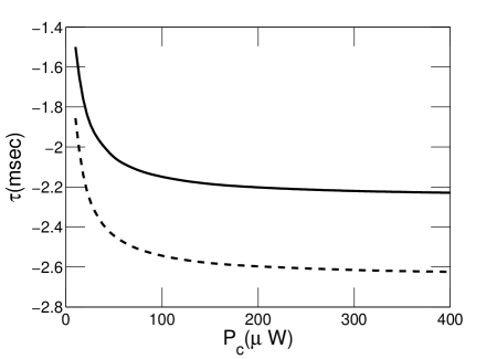
Figure 4: Group delay as a function of the pump power. Time delay of the probe in the presence of the coupling field as a function of the power of the pumping or coupling field with $\delta=\omega_{m}$. The solid and dashed lines are for $\gamma_{m}=2\pi\times 141$ Hz and $\gamma_{m}=2\pi\times 120$ Hz, respectively. The other parameters are the same with those of Fig.2.

.

We find large negative group delays of order $-2$ msec in a high quality cavity under the action of a coupling laser and a probe laser. In Fig.(4) the group delay is negative, as a result the fast light effect can be observed. This corresponds to a superluminal situation. In Fig.(4) the solid curve is for $\gamma_{m}=2\pi 141$ Hz and the dashed curve is for $\gamma_{m}=2\pi 120$ Hz. As the damped rate of the mirror decreases, the group delay increases at all pump powers, however after a critical value the group delays become approximately constant.

IV Conclusion

We have examined the question of advance of the pulse under the conditions of electromagnetically induced transparency in the mechanical system contained in a high quality cavity. We have investigated the tunable group delay of optical pulse in a nanomechanical one-sided cavity system and also we have explored the effect of the pump field power on the group delay. As the strength of the pump power increases the group delay becomes negatively larger. However, at a critical value of pump field power, group delay becomes approximately constant. Moreover, the dependence of the phase of the transmitted probe pulse on the frequency has been computed. In the absence of the coupling field, the group delay time is $\tau_{0}=2/\kappa=1.48\mu$sec. Whereas the magnitude of the group delay is on the order of $-2$ msec at a high pump power such as $400\mu$W for the parameters chosen in Ref.aspel . One can interpret that EIT reverses the behavior of the nanomechanical system. Superluminal light can be observed experimentally in a one-sided cavity system by adjusting the pump power. Our results may be used for measuring the fast light in a nanomechanical medium by comparing the group delay of the probe pulse with a reference pulse propagating in the absence of medium.

- (1) L.V. Hau, S.E. Harris, Z. Dutton, and C.H. Behroozi, Nature 397, 594 (1999).
- (2) S. E. Harris, Physics Today 50, 36 (1997).
- (3) M. D. Lukin, Rev. Mod. Phys. 75, 457 (2003).
- (4) M. Fleischhauer, A. Imamoglu, and J. P. Marangos, Rev. Mod. Phys. 77, 633 (2005).
- (5) M. D. Lukin and A. Imamoglu, Phys. Rev. Lett. 84, 1419 (2000).
- (6) M. S. Bigelow, N. N. Lepeshkin, and R. W. Boyd, Phys. Rev. Lett. 90, 113903 (2003).
- (7) L. J. Wang, A. Kuzmich, and A. Dogariu, Nature 406, 277 (2000).
- (8) A. Dogariu, A. Kuzmich, and L. J. Wang Phys. Rev. A 63, 053806 (2001).
- (9) M. S. Bigelow, N. N. Lepeshkin, and R. W. Boyd, Science 301, 200 (2003).
- (10) A. H. Safavi-Naeini, T. P. Alegre, J. Chan, M. Eichenfield, M. Winger, Q. Lin, J. T. Hill, D. E. Chang, and O. Painter, Nature 472, 69 (2011).
- (11) D. E. Chang, A. H. Safavi-Naeini, M. Hafezi and O. Painter, New J. Phys. 13, 023003 (2011).
- (12) I. Favero, and K. Karrai, Nature Photonics 3, 201 (2009).
- (13) A. Schliesser, R. Rivière, G. Anetsberger, O. Arcizet, and T. J. Kippenberg, Nature Physics 4, 415 (2008).
- (14) S. Gröblacher, K. Hammerer, M. Vanner, and M. Aspelmeyer, Nature 460, 724 (2009).
- (15) M. Bhattacharya, and P. Meystre, Phys. Rev. Lett. 99, 073601 (2007).
- (16) S. Weis, R. Riviere, S. Deleglise, E. Gavartin, O. Arcizet, A. Schliesser, and T. J. Kippenberg, Science 330, 1520 (2010).
- (17) A. Nunnenkamp, K. Borkje, and S. M. Girvin, Phys. Rev. Lett. 107, 063602 (2011).
- (18) T. Rocheleau, T. Ndukum, C. Macklin, J. B. Hertzberg, A. A. Clerk, and K. C. Schwab, Nature 463, 72 (2010).
- (19) G. S. Agarwal, and S. Huang, Phys. Rev. A 81, 041803(R) (2010).
- (20) M. Karuza, C. Biancofiore, C. Molinelli, M. Galassi, R. Natali, P. Tombesi, G. Di Giuseppe, and D. Vitali, arXiv:1209.1352 (2012).
- (21) V. Fiore, C. Dong, M. C. Kuzyk, and H. Wang, Phys. Rev. A 87, 023812 (2013).
- (22) V. Fiore, Y. Yang, M. C. Kuzyk, R. Barbour, L. Tian, and H. Wang, Phys. Rev. Lett. 107, 133601 (2011).
- (23) Y. Han, J. Cheng and L. Zhou, J. Phys. B: At. Mol. Opt. Phys. 44, 165505 (2010).
- (24) B. Chen, C. Jiang, and Ka-di Zhu, Phys. Rev. A 83, 055803 (2011).
- (25) C. Jiang, B. Chen, and Ka-di Zhu, Euro Phys. Lett. 94, 38002 (2011).
- (26) F. Marquardt, and S. M. Girvin, Physics 2, 40 (2009).
- (27) D. Vitali, S. Gigan, A. Ferreira, H. R. Böhm, P. Tombesi, A. Guerreiro, V. Vedral, A. Zeilinger, and M. Aspelmeyer, Phys. Rev. Lett. 98, 030405 (2007).
- (28) S. Huang, and G. S. Agarwal, New J. Phys 11, 103044 (2009).
- (29) S. Huang, and G. S. Agarwal, Phys. Rev. A 81, 033830 (2010).
- (30) M. J. Collet, and C. W. Gardiner, Phys. Rev. A 30, 1386 (1984).
- (31) R. Boyd, Nonlinear Optics, Academic Press, Amsterdam, 2008.