Replacing standard galaxy profiles with
mixtures of Gaussians

Abstract

Exponential, de Vaucouleurs, and Sérsic profiles are simple and successful models for fitting two-dimensional images of galaxies. One numerical issue encountered in this kind of fitting is the pixel rendering and convolution (or correlation) of the models with the telescope point-spread function (PSF); these operations are slow, and easy to get slightly wrong at small radii. Here we exploit the realization that these models can be approximated to arbitrary accuracy with a mixture (linear superposition) of two-dimensional Gaussians (MoGs). MoGs are fast to render and fast to affine-transform. Most importantly, if you have a MoG model for the pixel-convolved PSF, the PSF-convolved, affine-transformed galaxy models are themselves MoGs and therefore very fast to compute, integrate, and render precisely. We present worked examples that can be directly used in image fitting; we are using them ourselves. The MoG profiles we provide can be swapped in to replace the standard models in any image-fitting code; they sped up model fitting in our projects by an order of magnitude; they ought to make any code faster at essentially no cost in precision.

Gaussians are remarkable distribution functions. They have the incredible properties that—in any number of dimensions—the convolution (or correlation) of one multivariate Gaussian with another is itself a multivariate Gaussian, and any product of multivariate Gaussians is itself a multivariate Gaussian but with a different normalization. Furthermore, the means and variance tensors of the Gaussians output by these operations are related simply to the means and variance tensors of the inputs. Add to these wonders the fact that Gaussians form a complete basis for representing (smooth) probability distribution functions and it becomes remarkable that we don’t do everything we do in terms of Gaussians.

To elaborate, a mixture of multivariate Gaussians—a linear superposition—can be used to represent any reasonable distribution in any number of dimensions to any reasonable precision. Convolution (or correlation) by any other distribution that has also been represented by a mixture of multivariate Gaussians creates a new mixture of Gaussians with simply adjusted amplitudes, means, and variance tensors. The ubiquity of convolution operations in astronomy suggests the widespread adoption of mixture-of-Gaussian (MoG) modeling. We have pioneered this in the area of distribution modeling in large numbers of dimensions (Bovy et al. 2011a, b, 2012), where convolution occurs because the true or noise-free distribution is convolved with the noise before being observed. Here we are going to capitalize on the convolution properties of MoGs in modeling galaxy morphologies in imaging data, where the true or high-angular-resolution intensity field is convolved with the point-spread function (PSF) before being observed. This is always easier with Gaussians than cuspy profiles, but is particularly useful in data sets in which the PSF itself has also been modeled as a MoG, which is not uncommon (for example, the Sloan Digital Sky Survey imaging pipelines described by Lupton et al. 2001 make approximate MoG PSF models for every imaging field).

We are not the first in this space: Deconvolution and modeling of galaxy images with MoGs has been done very successfully before (for example, Bendinelli 1991; Emsellem et al. 1994; Bendinelli & Parmeggiani 1995; Cappellari 2002; they use the name “multi-Gaussian expansion” or MGE). However, the idea behind those projects was to use the MoGs to provide a very free form for the isophotes or morphologies of resolved galaxies or other complex scenes. Here our goals are very limited: We want to improve the performance of standard galaxy image model fitting by expressing the standard galaxy models—the exponential and de Vaucouleurs profiles—as rigid MoGs.

Whenever an investigator is fitting PSF-convolved exponential or de Vaucouleurs profiles, the models presented here will improve code performance. That doesn’t mean that doing such fitting is a Good Idea. These profiles are effective models for galaxies at low signal-to-noise (as they are used in the SDSS) and they are useful templates for performing consistent photometry across morphologically diverse objects (as we use them in Bundy et al. 2012). More radically, these profiles are sometimes used to distinguish disk and bulge light (as in Simard et al. 2011 and references cited therein); these uses are prone to over-interpretation: There is no theoretical argument and only weak observational arguments that the rotation-supported parts of galaxies are always exponential and that the kinematically hot components are always more de-Vaucouleurs-like.

The performance advantages we will obtain from using MoG approximations are not simply that convolution itself is trivial. The standard unconvolved galaxy models, especially the de Vaucouleurs and Sérsic models (de Vaucouleurs 1948, Sérsic 1963), are very ill-behaved near the galaxy center. Rendering these profiles precisely near the center can be very challenging numerically. In addition, most of the rendering time is spent at very small radii, where PSF convolution is going to erase all structure anyway. That is, a MoG description of the de Vaucouleurs profile saves time both in rendering and in PSF convolution; it produces profiles that are approximate but very high performance when all real uses of the profiles are PSF-convolved, as they usually are.

On the subject of PSF-convolution, it is important in any image-modeling situation to think of the PSF as the pixel-convolved point-spread function. Under this choice, synthesis of a pixelized image involves only convolution with the PSF and evaluation at the pixel centers. That is, image synthesis (returned to at the end of this Note) consists of PSF convolution—an arithmetic operation on the two MoGs—followed by evaluation of the resulting MoG at the pixel centers).

We need good performance in two-dimensional image synthesis (for fitting) because, with The Tractor (Lang et al., forthcoming), we are building a comprehensive model of all the imaging data we have; this will have models of many millions of galaxies in imaging that contains on the order of $10^{13}$ pixels. We are basing our models on the Sloan Digital Sky Survey (SDSS) Catalog galaxy models, which only include exponential, de Vaucouleurs, and composite (mixture of the two) radial profiles. In detail, in fact, the SDSS Catalog models are small modifications of these; details below. So our goal here is to provide replacements for these models in order to improve the performance of galaxy image modeling and analysis software. Some of the models we present have been used previously in tools for precise photometry (Bundy et al. 2012), and are being used in the Large Synoptic Survey Telescope (LSST) prototype galaxy photometry pipeline (Shaw 2012), in which these models are convolved with a shapelet representation of the PSF; because shapelets are simply polynomial perturbations on a Gaussian, they can also be convolved analytically with mixture-of-Gaussian galaxy models (Bosch 2010). These models could also be used to speed other image-fitting systems, like the very successful GALFIT (Peng et al. 2002). An alternative to making MoG profiles is to find exact analytic expressions for certain kinds of convolutions. There are some analytic results for PSF-convolved Sérsic models but they involve some non-trivial series and special-function expressions (Trujillo et al. 2001); we won’t come back to these again but they might be very useful in many situations.

Because we are thinking about two-dimensional imaging, we use here two-dimensional Gaussian or Normal distributions, which look like

$$\displaystyle N(\boldsymbol{x}\,|\,\boldsymbol{m},\boldsymbol{V}) \equiv \frac{1}{2\pi}\,\det(\boldsymbol{V})^{-1/2}\,\exp(-\frac{1}{2}\,{[\boldsymbol{x}-\boldsymbol{m}]}^{\mathsf{T}}\cdot{\boldsymbol{V}}^{-1}\cdot[\boldsymbol{x}-\boldsymbol{m}])\quad,$$ (1)

where $\boldsymbol{x}$ and $\boldsymbol{m}$ are two-dimensional vectors (usually in the focal plane or on the sky or something like that), and $\boldsymbol{V}$ is a symmetric $2\times 2$ variance tensor or matrix, and implicitly the vectors are column vectors. A mixture of Gaussians is a linear superposition of Gaussians. Any positive two-dimensional function with finite support and finite total integral—including as a special case any two-dimensional probability distribution function—can be represented as a MoG to arbitrary accuracy; that is

$$p(\boldsymbol{x}) \approx \sum_{k=1}^{K}a_{k}\,N(\boldsymbol{x}\,|\,\boldsymbol{m}_{k},\boldsymbol{V}_{k})$$ (2)

$$1 = \sum_{k=1}^{K}a_{k}\quad,$$ (3)

where $p(\boldsymbol{x})$ is any probability distribution of a two-dimensional quantity $\boldsymbol{x}$, the $\approx$ symbol implies approximation, $K$ is the number of Gaussians used in the MoG, and the $K$ Gaussians have amplitudes $a_{k}$, means $\boldsymbol{m}_{k}$, and variance tensors $\boldsymbol{V}_{k}$. The sum-to-one condition ensures that the probability distribution approximation is properly normalized.

We wish to make an approximation to the two-dimensional circular exponential (exp) profile $Q^{\exp}(\cdot)$

$$\displaystyle Q^{\exp}(\boldsymbol{\xi}) \equiv \exp(-\alpha^{\exp}\,[|\boldsymbol{\xi}|-1])$$ (4)

$$\alpha^{\exp} \equiv 1.67834699\quad,$$ (5)

where $\boldsymbol{\xi}$ is a dimensionless focal-plane position, and $\alpha^{\exp}$ is a dimensionless inverse length set to ensure that the profile has unit half-light radius. The position $\boldsymbol{\xi}$ is dimensionless because it parameterizes the unit-size dimensionless function. We seek the best (where “best” will be defined below) $M^{\exp}$-Gaussian MoG (where $M^{\exp}$ is an integer) approximation

$$\displaystyle Q^{\exp}(\boldsymbol{\xi}) \approx \sum_{m=1}^{M^{\exp}}a^{\exp}_{m}\,N(\boldsymbol{\xi}\,|\,\boldsymbol{0},\boldsymbol{V}^{\exp}_{m})$$ (6)

$$\boldsymbol{V}^{\exp}_{m} \equiv v^{\exp}_{m}\,\boldsymbol{I}\quad,$$ (7)

where all of the means are exactly zero and all of the variances $\boldsymbol{V}^{\exp}_{m}$ in the MoG can be represented as a scalar $v^{\exp}_{m}$ multiplied by the identity matrix $\boldsymbol{I}$ because we are requiring this dimensionless function to be precisely circular (so every component is itself circular and concentric). Similarly for the de Vaucouleurs (dev) profile

$$\displaystyle Q^{\mathrm{dev}}(\boldsymbol{\xi}) \equiv \exp(-\alpha^{\mathrm{dev}}\,[|\boldsymbol{\xi}|^{1/4}-1])$$ (8)

$$\alpha^{\mathrm{dev}} \equiv 7.66924944$$ (9)

$$Q^{\mathrm{dev}}(\boldsymbol{\xi}) \approx \sum_{m=1}^{M^{\mathrm{dev}}}a^{\mathrm{dev}}_{m}\,N(\boldsymbol{\xi}\,|\,\boldsymbol{0},\boldsymbol{V}^{\mathrm{dev}}_{m})$$ (10)

$$\boldsymbol{V}^{\mathrm{dev}}_{m} \equiv v^{\mathrm{dev}}_{m}\,\boldsymbol{I}\quad.$$ (11)

The half-light inverse-radius parameters $\alpha^{\exp}$ and $\alpha^{\mathrm{dev}}$ are from Ciotti & Bertin (1999). The challenge we meet below is to determine the parameters

$$\{a^{\exp}_{m},v^{\exp}_{m}\}_{m=1}^{M^{\exp}}~{},~{}\{a^{\mathrm{dev}}_{m},v^{\mathrm{dev}}_{m}\}_{m=1}^{M^{\mathrm{dev}}}$$ (12)

to best approximate the traditional galaxy profile functions, under some sensible definition of the word “best”, as a function of the model complexity parameters (numbers of components) $(M^{\exp},M^{\mathrm{dev}})$.

In addition to these, there are general Sérsic (“ser”) profiles, of which the exp and dev profiles are special cases. The general ser profile has one parameter (the “index”) $n$:

$$\displaystyle Q^{\mathrm{ser}(n)}(\boldsymbol{\xi}) \equiv \exp(-\alpha^{\mathrm{ser}(n)}\,[|\boldsymbol{\xi}|^{1/n}-1])$$ (13)

$$\{\alpha^{\mathrm{ser}(2)},\alpha^{\mathrm{ser}(3)},\alpha^{\mathrm{ser}(5)}\} \equiv \{3.67206075,5.67016119,9.66871461\}\quad,$$ (14)

where we have given the constant $\alpha^{\mathrm{ser}(n)}$ for just a few values of $n$ (Ciotti & Bertin 1999; the $\exp$ and $\mathrm{dev}$ profiles given above provide values for $n=1$ and $n=4$.)

The SDSS pipelines (Lupton et al. 2001) make use of modified profiles, which have been truncated smoothly at large radius and (in the case of the de Vaucouleurs profile) “softened” at the center. The SDSS form of the exponential (lux) profile is

$$\displaystyle Q^{\mathrm{lux}}(\boldsymbol{\xi}) \equiv \left\{\begin{array}[]{ll}\exp(-\alpha^{\mathrm{lux}}\,[|\boldsymbol{\xi}|-1])&\mbox{for~{}}|\boldsymbol{\xi}|<3\\ \exp(-\alpha^{\mathrm{lux}}\,[|\boldsymbol{\xi}|-1])\,\left[1-[|\boldsymbol{\xi}|-3]^{2}\right]^{2}&\mbox{for~{}}3<|\boldsymbol{\xi}|<4\\ 0&\mbox{for~{}}4<|\boldsymbol{\xi}|\end{array}\right.$$ (18)

$$\alpha^{\mathrm{lux}} \equiv 1.67835\quad,$$ (19)

and the SDSS form of the de Vaucouleurs (luv) profile is

$$\displaystyle Q^{\mathrm{luv}}(\boldsymbol{\xi}) \equiv \left\{\begin{array}[]{ll}\exp(-\alpha^{\mathrm{luv}}\,\left[[|\boldsymbol{\xi}|^{2}+0.0004]^{1/8}-1\right])&\mbox{for~{}}|\boldsymbol{\xi}|<7\\ \exp(-\alpha^{\mathrm{luv}}\,\left[[|\boldsymbol{\xi}|^{2}+0.0004]^{1/8}-1\right])\,\left[1-[|\boldsymbol{\xi}|-7]^{2}\right]^{2}&\mbox{for~{}}7<|\boldsymbol{\xi}|<8\\ 0&\mbox{for~{}}8<|\boldsymbol{\xi}|\end{array}\right.$$ (23)

$$\alpha^{\mathrm{luv}} \equiv 7.66925\quad.$$ (24)

The half-light inverse-radius parameters $\alpha^{\exp}$ and $\alpha^{\mathrm{dev}}$—and the softening and cutoff radius parameters—are taken from the SDSS codebase.

The profiles above are normalized to have unit intensity (approximately) at their half-light radii. In many cases, the investigator wants profiles that are normalized to have unit total flux (intensity integrated over solid angle). Although there is an analytic result for the dev profile, numerical integration of the concentrated profiles dev and luv to determine total fluxes can be challenging. This is not true for the MoG approximations: Each Gaussian is normalized, so the sum of the amplitudes $\sum_{m}a^{\mathrm{luv}}_{m}$ (for the luv profile, say) gives the total flux for the MoG approximation to that profile.

We seek the best MoG approximations. This necessitates definition of the word “best”. If we think of the profiles as being two-dimensional probability distribution functions (for, say, the arrivals of photons), then one natural choice is the K-L divergence or similar cross-entropy or information-theoretic measure. However, in typical astronomical imaging, the galaxy is superimposed on a substantial, flat sky level, and the noise in the data is close to Gaussian. This suggests more chi-squared-like objectives. We adopt the latter, in part because they are most appropriate for our specific proposed application (modeling SDSS-like astronomical imaging), but experiments we have performed suggest that information-theoretic objectives also lead to good results.

In detail, the chi-squared objective we minimize—the badness—is a squared residual between the exact profile function $Q(\boldsymbol{\xi})$ and its MoG approximation. It is designed to be equivalent to a chi-squared statistic in a homoskedastic two-dimensional image of the profile taken with extremely high angular resolution (pixels of size 0.001 the half-light radius) and vanishing point-spread function. Quantitatively the badness is defined to be the mean squared residual in the $Q(\boldsymbol{\xi})$ functions, which are normalized to have unit intensity at the half-light radius, averaged over a two-dimensional circular region in the $\boldsymbol{\xi}$ plane centered on the (circularly symmetric) profile and extending out to radius $\xi_{\max}$. We use $\xi_{\max}=8$ for all profiles except the $\mathrm{lux}$ profile, for which we use $\xi_{\max}=4$. In practice, the badness is computed in a one-dimensional numerical integral but the integral is weighted in radius (weight increasing linearly with radius) to make it equivalent to the two-dimensional chi-squared. We also add to the badness a very tiny coefficient (on the order of $10^{-3}$ of the best-fit badness) times the sum of the variances $v_{m}$ for regularization. In practice, this term doesn’t have much effect and could be dropped.

Optimization (minimization) of the badness is performed by the scipy implementation of the BFGS algorithm, with many initializations to explore multiple local minima. Further details are available in the code, which is publicly available.

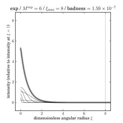
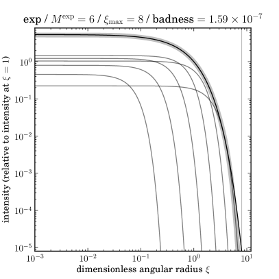
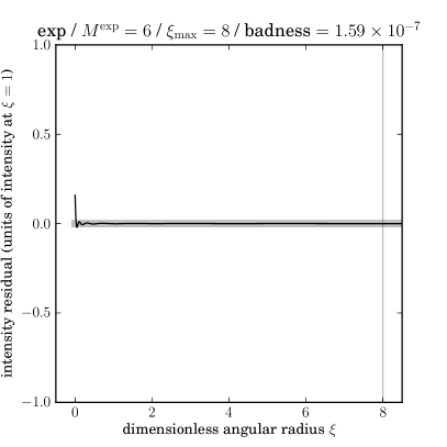
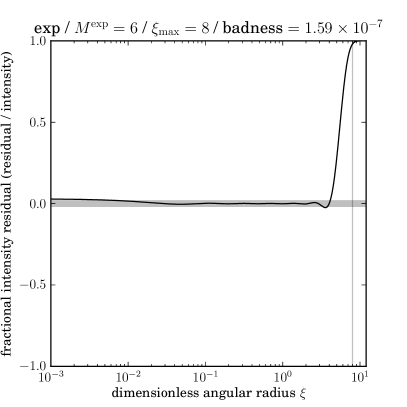
Figure 1: top-left: The true exp profile (thin black line), the best $M^{\exp}=6$ mixture-of-Gaussian approximation (thick grey line), and the component Gaussians (multiplied by their corresponding amplitudes) contributing to the approximation (thin grey lines). The plot title text gives $\xi_{\max}$ and the badness. top-right: The same but shown logarithmically. bottom-left: A representation of the residual or devation, on which the badness is computed. bottom-right: The same but shown fractionally and logarithmically.

The results of the optimizations are shown in Tables 1 and 2 and Figures 1 through 5. All the results shown in these figures and tables and more are available in machine-readable form from author DWH upon request. In the Tables and Figures we show root-variances rather than variances because these have units of half-light radii; they are simple standard deviations for the Gaussian components.

In our work on The Tractor, we use the $M^{\mathrm{lux}}=6$ lux and the $M^{\mathrm{luv}}=8$ luv profiles. Our advice to users would be to do the same. We use the lux and luv over the exp and dev partly because of their better behaviors numerically, and partly because they and we are both part of the SDSS tradition. These—$M^{\mathrm{lux}}=6$ and $M^{\mathrm{luv}}=8$—are good compromises between mixture complexity ($M$) and quality of fit (badness). Also, even the best-fitting late-type and early-type galaxies deviate from exponential and de Vaucouleurs fits by more than do these high-quality MoG approximations; no precision is lost.

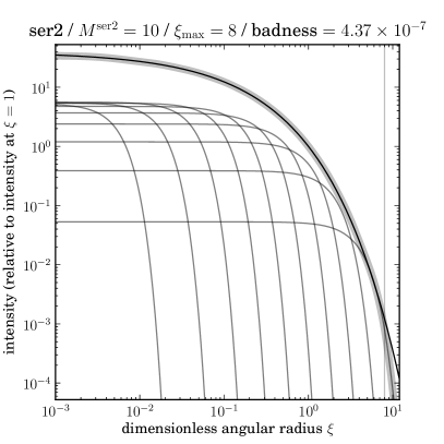
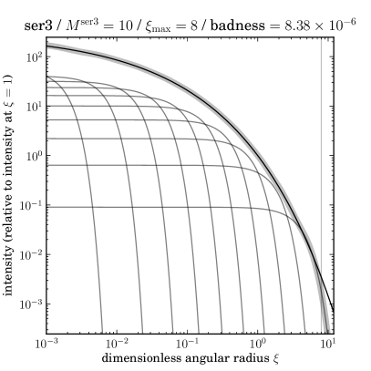
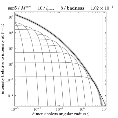
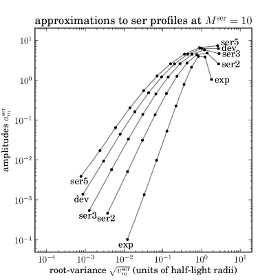
Figure 4: Three ser profiles—with $n=2$, $3$, and $5$—and approximations. The top-left, top-right, and bottom-left panels are equivalent to those in the top-right of Figure 1. bottom-right: The dependence on the amplitudes $a^{\mathrm{ser}(n)}_{m}$ and root-variances $\sqrt{v^{\mathrm{ser}(n)}_{m}}$ on ser index $n$.

In Figure 4, we show the dependence of amplitudes $a^{\mathrm{ser}(n)}_{m}$ and variances $v^{\mathrm{ser}(n)}_{m}$ on the ser index $n$. There is clearly continuity; a valuable follow-up project would be to give expressions for the amplitudes and variances as a function of ser index $n$. In the absence of cleverness our advice would be to make use of smooth interpolation.

The value of these MoG approximations comes when they are to be convolved with a PSF (usually in fact a pixel-convolved PSF) that is itself also represented as a MoG. In this scenario, the PSF $\psi(\Delta\boldsymbol{x})$—which is thought of as a function of focal-plane displacement $\Delta\boldsymbol{x}$ away from, say, a true stellar position—is represented as a $K$-Gaussian MoG

$$\displaystyle\psi(\Delta\boldsymbol{x}) = \sum_{k=1}^{K}p_{k}\,N(\Delta\boldsymbol{x}\,|\,\boldsymbol{m}_{k},\boldsymbol{V}_{k})$$ (25)

$$1 = \sum_{k=1}^{K}p_{k}\quad,$$ (26)

where the means $\boldsymbol{m}_{k}$ are not required to vanish because the PSF can have arbitrarily non-trivial structure (think speckles and the like) and the variances $\boldsymbol{V}_{k}$ will not in general be proportional to the identity or even diagonal because the PSF will not in general be round. An example that illustrates the use of this PSF is the following: A star of flux $S_{s}$ at focal-plane position $\boldsymbol{x}_{s}$ will lead to an image (PSF-convolved intensity map) of the form

$$\displaystyle I(\boldsymbol{x}\,|\,\mathrm{star},S_{s},\boldsymbol{x}_{s}) = \sum_{k=1}^{K}S_{s}\,p_{k}\,N(\boldsymbol{x}\,|\,\boldsymbol{x}_{s}+\boldsymbol{m}_{k},\boldsymbol{V}_{k})\quad.$$ (27)

That is, when the PSF is represented as a MoG, any image of a star—or indeed any image of any set of stars—is also represented as a MoG.

Applying this PSF to an exp or dev galaxy is slightly more complicated, because the galaxy has not just a flux $S_{g}$ and a central position $\boldsymbol{x}_{g}$; it also has a shape. Because we are only considering these simple galaxies, we are only permitting ellipsoidal shapes, which can be represented by a semi-major axis $a$, a semi-minor axis $b$, and a position angle $\phi$, or equivalently by eigenvalues $a,b$ and eigenvectors $\boldsymbol{u}_{1},\boldsymbol{u}_{2}$, or equivalently by an affine transformation $\boldsymbol{R}_{g}$ that takes a circle to the relevant ellipse (and is therefore a general representation of an ellipse; it is also the matrix square root of the symmetric variance tensor describing the ellipse). The galaxy is distorted by this affine transformation prior to PSF convolution, so the focal-plane image (PSF-convolved intensity field) for a general (say) $\exp$ galaxy is given by

$$\displaystyle I(\boldsymbol{x}\,|\,\exp,S_{g},\boldsymbol{x}_{g},\boldsymbol{R}_{g}) = \sum_{k=1}^{K}\sum_{m=1}^{M^{\exp}}S_{g}\,a^{\exp}_{m}\,p_{k}\,N(\boldsymbol{x}\,|\,\boldsymbol{x}_{g}+\boldsymbol{m}_{k},\boldsymbol{V}_{gm}+\boldsymbol{V}_{k})$$ (28)

$$\boldsymbol{V}_{gm} \equiv \boldsymbol{R}_{g}\cdot\boldsymbol{V}^{\exp}_{m}\cdot{\boldsymbol{R}_{g}}^{\mathsf{T}}$$ (29)

$$\boldsymbol{R}_{g} = \left[a\,\boldsymbol{u}_{1},b\,\boldsymbol{u}_{2}\right]\quad,$$ (30)

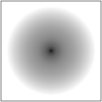
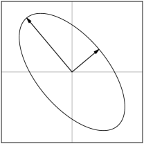
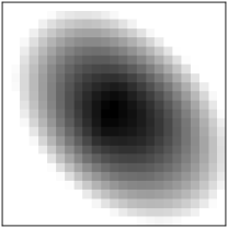
Figure 6: Demonstration of use of the profiles, or the implicit generative model in this Note. top-left: The circular dimensionless $M^{\mathrm{luv}}=8$ mixture-of-Gaussian approximation to the luv profile, represented on a very fine pixel grid. top-right: The ellipse representing the non-trivial affine transformation to be applied to the circular, dimensionless profile. middle-left: The sheared profile. middle-right: A $K=3$ mixture-of-Gaussian model of the pixel-convolved point-spread function, represented on the very fine pixel grid. bottom-left: The sheared profile convolved with the PSF, represented on the very fine pixel grid. bottom-right: The sheared luv convolved with the PSF, but now shown on a realistic pixel grid. Because by assumption the PSF is a pixel-convolved PSF, the representation on the realistic grid is found simply by interpolating to the pixel centers the mixture-component Gaussians.

where $a$ and $b$ are the major and minor axis lengths of the galaxy ellipse (in appropriate units) and $\boldsymbol{u}_{1}$ and $\boldsymbol{u}_{2}$ are the eigenvectors in image coordinates pointing in the major-axis and minor-axis directions respectively. Implicitly all vectors are two-dimensional column vectors, and $\boldsymbol{R}_{g}$ is a $2\times 2$ affine transformation matrix that contains the “shape” (position angle, major-axis, and ellipticity) information about the galaxy. The $\mathrm{dev}$, $\mathrm{ser}(n)$, $\mathrm{luv}$, and $\mathrm{lux}$ cases are all essentially the same. Note the important and key result of this Note, to wit, that a MoG galaxy model (with $M$ components) convolved with a MoG PSF model (with $K$ components) yields a MoG model image (with $[M\,K]$ components). In Figure 6 we show how we are using these MoG approximations in The Tractor—a generative modeling framework for measuring astronomical objects—to render PSF-convolved galaxy images.

In the above we said “pixel-convolved PSF”. In every context, when modeling images, it is valuable to use the pixel-convolved PSF. With this definition of the PSF, the pixelized image is the PSF-convolved true model evaluated at the pixel centers. This operation is fast. Other definitions for the PSF (the non-pixel-convolved, for example) require that the user do two convolutions, the first with the PSF and the second with the square (or worse) pixel. Our advice: Only fit for and use pixel-convolved PSFs.

If your PSF is not in MoG form, it is still the case that convolution of a MoG approximation of a dev (say) profile will in general be easier than convolution of the original dev profile. The reason is that convolution of a Gaussian with any PSF is fast (indeed most image-processing languages have such functions built in); the PSF-convolved profile becomes in this case just a mixture of Gaussian-convolved PSFs.

The speed-ups that can be obtained by using MoG approximations can be very large. In our image-modeling project The Tractor, we were PSF-convolving by rendering the profiles (especially the profile centers) at very high resolution (hundreds to thousands of resolution elements in the central pixel are necessary for good precision on the dev profile). We were then convolving that high-resolution model with a low-resolution PSF and rendering to a low-resolution image pixel grid. These expensive operations were obviated by the MoG profiles, which involve only rendering a small number of Gaussians at the pixel centers on the low-resolution pixel grid. The MoG approximations saved us more than an order of magnitude in compute time, especially in optimization, where derivatives have to be taken with respect to the unconvolved model properties.

In the SDSS, GALFIT, and much of our own work, the models that are fit are (effectively) mixtures of exp and dev or exp and ser or lux and luv profiles. Mixtures of profiles that are each themselves mixtures of Gaussians are no harder to render than either profile separately. There is some book-keeping, of course, because each component gets affine-transformed separately before they are both PSF-convolved.

One amusing aspect of MoG profiles has to do with projection from three to two dimensions. The projection of a three-dimensional Gaussian is a two-dimensional Gaussian; the two-dimensional, rigid, circular approximations we have made for the ser profiles can be deprojected to rigid, spherical approximations to the three-dimensional profiles trivially. The two-dimensional models we have started with are not accurate models of galaxies in detail—no galaxy follows exactly any ser profile—so deprojection of our approximations are not that interesting in themselves. However, the general program of fitting two-dimensional sources with MoGs may have strong implications in the future for three-dimensional modeling and deprojection.

	exp
$M^{\exp}=$	$4$		$6$		$8$
$m$	$a^{\exp}_{m}$	$\sqrt{v^{\exp}_{m}}$	$a^{\exp}_{m}$	$\sqrt{v^{\exp}_{m}}$	$a^{\exp}_{m}$	$\sqrt{v^{\exp}_{m}}$
$1$	$0.09733$	$0.12068$	$0.00735$	$0.05072$	$0.00077$	$0.02394$
$2$	$1.12804$	$0.32730$	$0.09481$	$0.13756$	$0.01017$	$0.06492$
$3$	$4.99846$	$0.68542$	$0.63572$	$0.28781$	$0.07313$	$0.13581$
$4$	$5.63632$	$1.28089$	$2.60077$	$0.53195$	$0.37184$	$0.25095$
$5$			$5.42848$	$0.91209$	$1.39736$	$0.42942$
$6$			$3.16445$	$1.50157$	$3.56100$	$0.69675$
$7$					$4.74338$	$1.08885$
$8$					$1.78684$	$1.67302$
$\sum_{m}a^{\exp}_{m}=$	$11.860$		$11.932$		$11.944$
badness $=$	$4.35\times 10^{-6}$		$1.59\times 10^{-7}$		$8.90\times 10^{-9}$

	dev
$M^{\mathrm{dev}}=$	$6$		$8$		$10$
$m$	$a^{\mathrm{dev}}_{m}$	$\sqrt{v^{\mathrm{dev}}_{m}}$	$a^{\mathrm{dev}}_{m}$	$\sqrt{v^{\mathrm{dev}}_{m}}$	$a^{\mathrm{dev}}_{m}$	$\sqrt{v^{\mathrm{dev}}_{m}}$
$1$	$0.01308$	$0.00263$	$0.00262$	$0.00113$	$0.00139$	$0.00087$
$2$	$0.12425$	$0.01202$	$0.02500$	$0.00475$	$0.00941$	$0.00296$
$3$	$0.63551$	$0.04031$	$0.13413$	$0.01462$	$0.04441$	$0.00792$
$4$	$2.22560$	$0.12128$	$0.51326$	$0.03930$	$0.16162$	$0.01902$
$5$	$5.63989$	$0.36229$	$1.52005$	$0.09926$	$0.48121$	$0.04289$
$6$	$9.81523$	$1.23604$	$3.56204$	$0.24699$	$1.20357$	$0.09351$
$7$			$6.44845$	$0.63883$	$2.54182$	$0.20168$
$8$			$8.10105$	$1.92560$	$4.46441$	$0.44126$
$9$					$6.22820$	$1.01833$
$10$					$6.15393$	$2.74555$
$\sum_{m}a^{\mathrm{dev}}_{m}=$	$18.454$		$20.307$		$21.290$
badness $=$	$2.01\times 10^{-3}$		$3.16\times 10^{-4}$		$3.90\times 10^{-5}$

Table 1: The amplitudes and root-variances for the best mixture-of-Gaussian approximations to the exp and dev profiles, for different mixture sizes. The total (dimensionless) fluxes and the badnesses are given for each approximation.

	lux
$M^{\mathrm{lux}}=$	$4$		$6$		$8$
$m$	$a^{\mathrm{lux}}_{m}$	$\sqrt{v^{\mathrm{lux}}_{m}}$	$a^{\mathrm{lux}}_{m}$	$\sqrt{v^{\mathrm{lux}}_{m}}$	$a^{\mathrm{lux}}_{m}$	$\sqrt{v^{\mathrm{lux}}_{m}}$
$1$	$0.07275$	$0.10938$	$0.00235$	$0.03465$	$0.00007$	$0.01092$
$2$	$0.86763$	$0.29694$	$0.03080$	$0.09405$	$0.00098$	$0.02966$
$3$	$4.33214$	$0.62601$	$0.22336$	$0.19785$	$0.00736$	$0.06241$
$4$	$6.48325$	$1.19571$	$1.17949$	$0.37413$	$0.04404$	$0.11794$
$5$			$4.33874$	$0.67894$	$0.24005$	$0.21345$
$6$			$5.99821$	$1.22540$	$1.18175$	$0.38155$
$7$					$4.31918$	$0.68169$
$8$					$5.97985$	$1.22635$
$\sum_{m}a^{\mathrm{lux}}_{m}=$	$11.756$		$11.773$		$11.773$
badness $=$	$1.37\times 10^{-5}$		$4.64\times 10^{-6}$		$4.55\times 10^{-6}$

	luv
$M^{\mathrm{luv}}=$	$6$		$8$		$10$
$m$	$a^{\mathrm{luv}}_{m}$	$\sqrt{v^{\mathrm{luv}}_{m}}$	$a^{\mathrm{luv}}_{m}$	$\sqrt{v^{\mathrm{luv}}_{m}}$	$a^{\mathrm{luv}}_{m}$	$\sqrt{v^{\mathrm{luv}}_{m}}$
$1$	$0.11960$	$0.01988$	$0.04263$	$0.01496$	$0.01468$	$0.01190$
$2$	$0.61327$	$0.05008$	$0.24013$	$0.03166$	$0.09627$	$0.02210$
$3$	$1.75843$	$0.12067$	$0.68591$	$0.06471$	$0.28454$	$0.03995$
$4$	$3.84242$	$0.28955$	$1.51937$	$0.13017$	$0.63005$	$0.07117$
$5$	$6.48187$	$0.72628$	$2.83627$	$0.26170$	$1.19909$	$0.12586$
$6$	$7.59437$	$2.12717$	$4.46467$	$0.53592$	$2.03195$	$0.22240$
$7$			$5.72441$	$1.15464$	$3.07255$	$0.39593$
$8$			$5.60990$	$2.89864$	$4.10682$	$0.71922$
$9$					$4.83948$	$1.37549$
$10$					$4.94943$	$3.13117$
$\sum_{m}a^{\mathrm{luv}}_{m}=$	$20.410$		$21.123$		$21.225$
badness $=$	$1.40\times 10^{-4}$		$8.42\times 10^{-6}$		$1.44\times 10^{-6}$

Table 2: Same as Table 1 but for the lux and luv profiles.

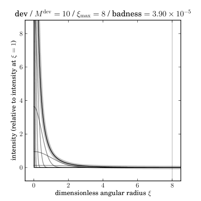
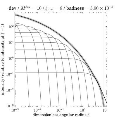
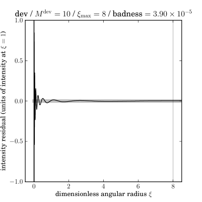
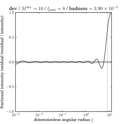
Figure 2: The dev profile and the best $M^{\mathrm{dev}}=10$ approximation. The panels are equivalent to those in Figure 1.

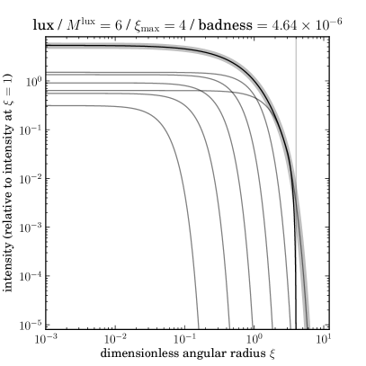
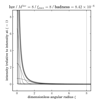
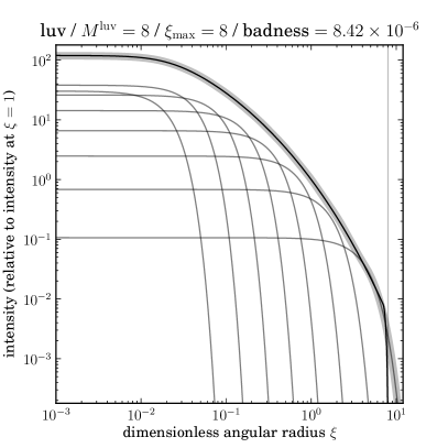
Figure 3: The lux and luv profiles and approximations. The panels are equivalent to those in the top-row of Figure 1.

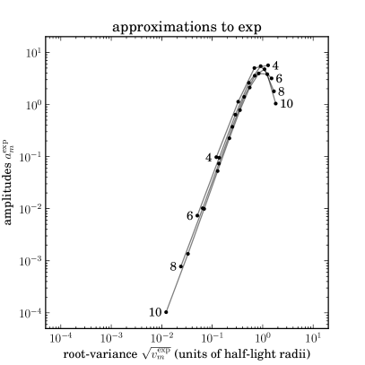
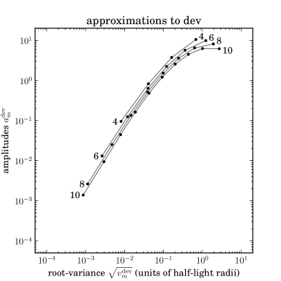
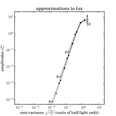
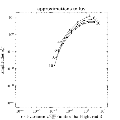
Figure 5: Comparisons of approximations. top-left: The dependence of amplitude $a^{\exp}_{m}$ and root-variance $\sqrt{v^{\exp}_{m}}$ on $M^{\exp}$ for the exp profile. top-right: The same but for the dev profile. bottom-left: The same but for the lux profile. bottom-right: The same but for the luv profile.

References

- Bendinelli (1991) Bendinelli, O., 1991, ApJ, 366, 599
- Bendinelli & Parmeggiani (1995) Bendinelli, O. & Parmeggiani, G., 1995, AJ, 109, 572
- Bosch (2010) Bosch, J., 2010, AJ, 140, 870
- Bovy et al. (2011a) Bovy, J., Hogg, D. W., & Roweis, S., 2011, Ann. Appl. Stat., 5, 1657
- Bovy et al. (2011b) Bovy, J., et al., 2011, ApJ, 729, 141
- Bovy et al. (2012) Bovy, J. et al., 2012, AJ, 749, 41
- Bundy et al. (2012) Bundy, K. et al., AJ, in press
- Cappellari (2002) Cappellari, M., 2002, MNRAS, 333, 400
- Ciotti & Bertin (1999) Ciotti, L. & Bertin, G., 1999, å, 352, 447
- de Vaucouleurs (1948) de Vaucouleurs, G., 1948, Annales d’Astrophysique, 11, 247
- Emsellem et al. (1994) Emsellem, E., Monnet, G., Bacon, R., & Nieto, J.-L., 1994, A&A, 285, 739
- Lupton et al. (2001) Lupton, R., Gunn, J. E., Ivezic, Z., Knapp, G. R., Kent, S. M., & Yasuda, N., 2001, ASPC, 238, 269
- Peng et al. (2002) Peng, C. Y., Ho, L. C., Impey, C. D., & Rix, H.-W., 2002, AJ, 124, 266
- Sérsic (1963) Sérsic, J. L., 1963, Boletin de la Asociacion Argentina de Astronomia La Plata Argentina, 6, 41
- Shaw (2012) Shaw, R. A., ed., 2012, LSST Data Challenge Handbook (Version 2.0; Tucson, AZ: LSST Corp.)
- Simard et al. (2011) Simard, L., Mendel, J. T., Patton, D. R., Ellison, S. L., & McConnachie, A. W., 2011, ApJS, 196, 11
- Trujillo et al. (2001) Trujillo, I., Aguerri, J. A. L., Cepa, J., & Gutiérrez, C. M., 2001, MNRAS, 321, 269