Magnetic Quantum Phase Diagram of Magnetic Impurities in 2 Dimensional Disordered Electron Systems

Abstract

The quantum phase diagram of disordered electron systems as function of the concentration of magnetic impurities $n_{m}$ and the local exchange coupling $J$ is studied in the dilute limit. We take into account the Anderson localisation of the electrons by a nonperturbative numerical treatment of the disorder potential. The competition between RKKY interaction $J_{\rm RKKY}$ and the Kondo effect, as governed by the temperature scale $T_{K}$, is known to gives rise to a rich magnetic quantum phase diagram, the Doniach diagram. Our numerical calculations show that in a disordered system both the Kondo temperature $T_{K}$ and $J_{\rm RKKY}$ are widely distributed. Accordingly, also their ratio, $J_{\rm RKKY}/T_{K}$ is widely distributed as shown in Fig. 1 (a). However, we find a sharp cutoff of that distribution, which allows us to define a critical density of magnetic impurities $n_{c}$ below which Kondo screening wins at all sites of the system above a critical coupling $J_{c}$, forming the Kondo phase [see Fig. 1 (b)]. As disorder is increased, $J_{c}$ increases and a spin coupled phase is found to grow at the expense of the Kondo phase. From these distribution functions we derive the magnetic susceptibility which show anomalous power law behavior. In the Kondo phase that power is determined by the wide distribution of the Kondo temperature, while in the spin coupled phase it is governed by the distribution of $J_{\rm RKKY}$. At low densities and small $J<J_{c}$ we identify a paramagnetic phase. We also report results on a honeycomb lattice, graphene, where we find that the spin coupled phase is more stable against Kondo screening, but is more easily destroyed by disorder into a PM phase.

I Introduction

Phenomena which emerge from the interplay of strong correlations and disorder remain a challenge for condensed matter theory. Spin correlations and disorder effects are however relevant for a wide range of materials, including doped semiconductors like Si:P close to metal-insulator transitions,v. Löhneysen (2000) and heavy Fermion systems, materials with 4f or 5f atoms, notably Ce, Yb, or U.Löhneysen et al. (2007) Many of these materials show a remarkable magnetic quantum phase transition which can be understood by the competition between indirect exchange interaction, the Ruderman-Kittel-Kasuya-Yoshida (RKKY) interaction between localised magnetic momentsRuderman and Kittel (1954); Kasuya (1956); Yosida (1957) and their Kondo screening.

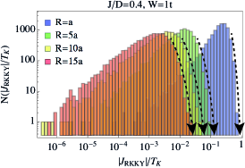
(a)                                         

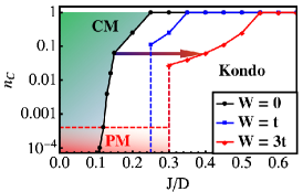
(b)                                         

Figure 1: (Color online) (a) Distribution of the ratio between $|J_{\rm RKKY}|$ and $T_{K}$ for various distances R. Black dashed arrow: sharp cutoff of each distribution (b) Magnetic quantum phase diagram: critical MI density $n_{c}$ as function of $J/D$ for various disorder strengths $W$ as determined by the distance $R$ below which $|J_{\rm RKKY}|/T_{K}$ does not exceed 1 at any site. Horizontal dashed line: density $n_{\xi}$ below which there is a paramagnetic moment phase (PM). CM= phase with coupled magnetic moments.

Thereby, one finds a suppression of long range magnetic order when exchange coupling $J$ is increased and Kondo screening succeeds. This results in a typical quantum phase diagram with a quantum critical point where the $T_{c}$ of the magnetic phase is vanishing, the Doniach diagram.Doniach (1977)

Recently, controlled studies of magnetic adatoms on the surface of metals,Zhou et al. (2010) on graphene,Chen et al. (2007) and on the conducting surface of topological insulatorsHsieh et al. (2009); Chen et al. (2010); Scholz et al. (2012); Seibel et al. (2012) with surface sensitive experimental methods like spin resolved STM and ARPES became possible. This demands a theoretical study of the Doniach diagram for magnetically doped disordered electron systems (DES), in particular 2D systems.

In any material there is some degree of disorder. In doped semiconductors it arises from the random positioning of the dopants themselves, in heavy Fermion metals and in 2D metals it may arise from structural defects or impurities. Disorder is known to cause Anderson localisation, which therefore has to be taken into account when deriving the Doniach diagram of disordered electrons systems. Moreover, as noted already early,Anderson (1977) the physics of random systems is fully described by probability distributions, not just averages. This must be particularly true for systems with random local magnetic impurities (MIs),Mott, N. F. (1976) since the magnetic impurities are exposed to the local density of states of the conduction electrons, which is widely distributed itself. In fact, it has been noticed that a wide distribution of the Kondo temperature $T_{K}$ of MIs in disordered host metals gives rise to non-Fermi liquid behavior, such as the low temperature power-law divergence of the magnetic susceptibility.Mott, N. F. (1976); Miranda and Dobrosavljevic (2005); Miranda et al. (1996); Bhatt and Fisher (1992); Langenfeld and Wölfle (1995); Castro Neto and Jones (2000); Cornaglia et al. (2006); Kettemann and Mucciolo (2007); Tran and Kim (2010) Nonmagnetic disorder quenches the Kondo screening of MIs due to Anderson-localisation and the formation of local pseudogaps at the Fermi energy,Kettemann and Mucciolo (2007); Zhuravlev et al. (2007); Kettemann and Raikh (2003); Kettemann et al. (2012) resulting in bimodal distributions of $T_{K}$ and a finite concentration of free, paramagnetic moments (PMs). However, in these studies the RKKY interaction $J_{\rm RKKY}$ between different MIs has not yet been taken into account. $J_{\rm RKKY}$ is mediated by the conduction electrons, and aligns the spins of the MIs ferromagnetically or antiferromagnetically, depending on their distance $R$. This is a long-ranged interaction, with a power law decay $J_{\rm RKKY}\sim 1/R^{d}$, where d is the dimension, and its typical value is not changed by weak disorder.Lerner (1993); Bulaevskii and Panyukov (1986); Bergmann (1987); Lee et al. (2012a) However, its amplitude has a wide log-normal distribution in disordered metals.Lerner (1993); Lee et al. (2012b) In this article we therefore intend to study the competition between RKKY interaction and the Kondo effect in disordered electron systems.

In the next section we introduce the model, and provide the equations for the Kondo temperature and the RKKY coupling. In section III, we derive numerically the distribution function of $J_{\rm RKKY}$, and compare it with an analytical result, based on a perturbative expansion of the nonlinear sigma model. We derive next numerically the distribution function of $T_{K}$ finding excellent agreement with approximate analytical results which were obtained, taking into account the multifracatlity and power law correlations of wave functions. In section IV we present the main results, the distribution function of the Ratio of TK and RKKY Interaction, for various distances between magnetic impurities R. From that we show how to derive the zero temperature magnetic quantum phase diagram as function of magnetic impurity density and exchange coupling, for 2D disordered electronic systems. At low densities and small $J<J_{c}$ we identify a paramagnetic phase. For graphene we find that the spin coupled phase is more stable against Kondo screening, but is more easily destroyed by disorder into a PM phase. In section V we derive from the distribution functions the magnetic susceptibility as function of temperature, which show anomalous power law behavior. In the Kondo phase that power is found to be determined by the wide distribution of the Kondo temperature, while at small exchange coupling there we identify spin coupled phase where the magnetic susceptibility is governed by the distribution of $J_{\rm RKKY}$. In the final section we conclude and discuss the relevance and limitations of our results.

II Model

In order to obtain the Doniach diagram of random electron systems we extend the approach of DoniachDoniach (1977) by calculating the distribution functions of $T_{K}$ and $J_{\rm RKKY}$ and their ratio. Thus, in our approach we try to draw conclusions on the quantum phase diagram of an electron system with a finite density of magnetic impurities, by considering the Kondo temperature of single impurities and the RKKY coupling of pairs of magnetic moments.

We start from a microscopic description of the MIs, the Anderson impurity model coupled to a non-interacting disordered electronic Hamiltonian with on-site disorder. Then, we map it with the Schrieffer-Wolff transformation on a model of Kondo impurity spins coupled to the disordered host electron spins by the local coupling $J$.Kettemann et al. (2012) We consider the single-impurity $T_{K}$ and the coupling $J_{\rm RKKY}$ between a pair of spins. For the numerical calculations we employ the single-band Anderson tight-binding model on a square lattice of size $L$ and lattice spacing $a$,

$$\centering H=-t\sum_{\langle i,j\rangle}c_{i}^{\dagger}c_{j}+\sum_{i}(w_{i}-\tilde{E}_{F})~{}c_{i}^{\dagger}c_{i},\@add@centering$$ (1)

where $t$ is the hopping energy between nearest neighbours $\langle i,j\rangle$, $w_{i}$ is the on-site disorder potential distributed in the interval $[-W/2,W/2]$. $\tilde{E}_{F}=E_{F}+\varepsilon_{\rm edge}$, where $E_{F}$ is the Fermi energy measured from the band edge, in 2D $\varepsilon_{\rm edge}=-4t$. We use periodic boundary conditions.

In the dilute limit, one can calculate the $T_{K}$ of a single magnetic impurity at position $\bm{R}_{i}$ from the Nagaoka-Suhl one-loop equation,Nagaoka (1965); Suhl (1965)

$$1=\frac{J}{2}\int_{0}^{D}d\varepsilon\,\frac{\tanh[(\varepsilon-E_{F})/2T_{K}]}{\varepsilon-E_{F}}\,\rho_{ii}(\varepsilon),$$ (2)

with band width $D$. $\rho_{ii}(\varepsilon)=\braket{i}{\delta(\varepsilon-H)}{i}$ is the local density of states (LDOS). The RKKY coupling $J_{{\rm RKKY}_{ij}}$ between two MIs located at positions $\bm{R}_{i}$,  $\bm{R}_{j}$ is in the zero temperature limit ($T=0$) given byRoche and Mayou (1999); Lee et al. (2012a)

$$J_{{\rm RKKY}_{ij}}=-J^{2}\frac{S(S+1)}{2S^{2}}\int_{\varepsilon<E_{F}}d\varepsilon\int_{\varepsilon^{\prime}>E_{F}}d\varepsilon^{\prime}\frac{F(\varepsilon,\varepsilon^{\prime})_{ij}}{\varepsilon-\varepsilon^{\prime}},$$ (3)

where $F(\varepsilon,\varepsilon^{\prime})_{ij}={\rm Re}[\rho_{ij}(\varepsilon)\rho_{ji}(\varepsilon^{\prime})]$, and $S$ is the magnitude of the MI spin.

III Distribution Functions

Using the Kernel Polynomial method (KPM),Roche and Mayou (1999); Weiße et al. (2006) one can evaluate the matrix elements of the density matrix $\rho_{ij}(\varepsilon)=\braket{i}{\delta(\varepsilon-\hat{H})}{j}$Lee et al. (2012a); Weiße et al. (2006); Mucciolo (2010) with a polynomial expansion of order $M$. Here, we increase the cutoff degree $M$ linearly with the linear system size $L$ based on our analysis for the convergence of RKKY interaction with respect $M$ in Ref. Lee et al., 2012b. It has been also carefully discussed in Ref. Wenk and Bouzerar, 2013 that the choice of $M\propto L$, not $M\propto L^{2}$, gives proper DOS and LDOS results avoiding finite size effect.

Eq. (3) yields in a clean 2D system

$$J^{0}_{\rm 2D}=-\frac{m^{*}}{8\pi}\sin(2k_{F}R)/(k_{F}R)^{2}$$

in the asymptotic limit $k_{F}R\gg 1$ with effective electron mass $m^{*}=1/(2a^{2}t)$ , and Fermi wave vector $k_{F}$. Ruderman and Kittel (1954) Its geometrical average is close to the clean limit for distances $R$ smaller than localisation length $\xi$, and decays exponentially at larger distances,Sobota et al. (2007); Lee et al. (2012a) $e^{{\langle\frac{1}{2}\ln J_{\rm RKKY}}^{2}\rangle}\sim e^{-R/\xi}.$ As shown in Figs. 2 a, b, the distribution of the absolute value of $J_{\rm RKKY}$ is well fitted by a log-normal,

$$N(x)=\frac{N}{\sqrt{2\pi\sigma}}\exp\left[-\frac{(x-x_{0})^{2}}{2\sigma^{2}}\right],$$

where $x=\ln|J_{\rm RKKY}|$ and the fitting gives for $R=5a$ and $W=2t,4t$, $x_{0}=5,6$ and width $\sigma=5.3+.85W/t$ increasing with the disorder strength $W$. This is qualitatively consistent with analytical results obtained at weak disorder,Lerner (1993) while analytical calculations at strong disorder have not been performed yet. This distribution width hardly depends on the distance $R$. We used $N=30\,000$ disorder configurations.

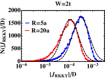
(a)

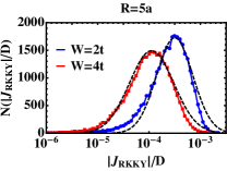
(b)

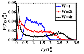
(c)

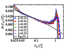
(d)

Figure 2: (Color online) $N(|J_{\rm RKKY}|)$ at (a) fixed disorder strength $W=2t$, (b) fixed $R=5a$ ($N=30\,000$, $L=100a$, $M=1000$). Black dashed lines: fit to log-normal distribution. (c) $P(T_{K})$ at fixed $j=J/D=0.25$, (d) $P(T_{K})$ at fixed $W=5t$ (N=30 000, L=40a, M=200). $E_{F}=2t$ in a)-d).

The distribution of $T_{K}$ is shown in Fig. 2 c, as obtained from the numerical solution of Eq. (2) for $L=40a$, $j=J/D=0.25$. Since for every sample only one single site is taken to avoid a distortion of the distribution due to intersite correlations, we had to use a huge number of $N=30\,000$ different random disorder configurations to get sufficient statistics. It has a strongly bimodal shape where the low $T_{K}$- peak becomes more distinctive with larger disorder amplitude $W$.Cornaglia et al. (2006); Kettemann and Mucciolo (2007, 2006) In Fig. 2 d we show these results for fixed disorder strength $W=5t$ for various exchange couplings $j$. Recently, an analytical derivation of the low $T_{K}$-tail of $P(T_{K})$ was done, using the multifractal distribution and correlations of intensities.Kettemann et al. (2012) These correlations are in 2D logarithmic with an amplitude of order $1/g$, where $g=E_{F}\tau$. For weak disorder, $g\gg 1$, it corresponds to a power law correlation with power $\eta_{2D}=2/\pi g.$ The correlation energy is of the order of the elastic scattering rate $E_{c}\sim 1/\tau$. Thus, for $T_{K}\ll{\rm Max}\{\Delta_{\xi}=D/\xi^{2},\Delta=D/L^{2}\}$,Kettemann et al. (2012)

$$P(T_{K})=\left(1-p_{FM}\right)\left(\frac{E_{c}}{T_{K}}\right)^{1-j}({\rm Min}\{\xi,L\})^{-\frac{d^{2}j^{2}}{2\eta_{2D}}},$$ (4)

where $p_{FM}=n_{FM}(0)/n=({\rm Min}\{\xi,L\})^{-\frac{d^{2}j^{2}}{2\eta_{2D}}}$, the ratio of free PMs. Eq. (4) has a power law tail with power $\beta_{j}=1-j$ in good agreement with the numerical results, Fig. 2 d, for $T_{K}/T_{K}^{0}<.03$. For $T_{K}^{0}>T_{K}>{\rm Max}\{\Delta_{\xi}=D/\xi^{2},\Delta=D/L^{2}\}$ one findsKettemann et al. (2012)

$$\frac{P(T_{K})}{1-p_{FM}}=(\frac{E_{c}}{T_{K}})^{1-\frac{\eta_{2D}}{2d}}\exp[-\frac{(\frac{T_{K}}{E_{c}})^{\frac{\eta_{2D}}{d}}}{2c_{1}}\ln^{2}\left(\frac{T_{K}}{T_{K}^{0}}\right)],$$ (5)

where $c_{1}=7.51$. This expression is in agreement with the numerical results, see Fig. 2 d, using $\xi=g\exp(\pi g)$, and $1/\tau=\pi W^{2}/6D$, fitting only $E_{c}\approx.73t$ and the prefactor. Thus, we confirm that the power law tail is governed by the multifractal correlation with power $\eta_{2D}$.

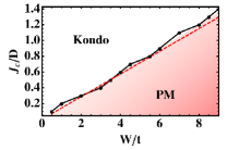
(a)

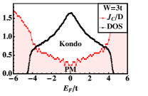
(b)

Figure 3: (Color online) Quantum phase diagram with paramagnetic moment phase (PM) and Kondo screened phase: Critical exchange coupling $J_{c}/D$ ($L=100$) (a) as function of $W$ ($M=300$,$E_{F}=2t$). Red dashed line: Eq. (6). (b) as function of Fermi energy $E_{F}$  ($M=200$); Red line:  (DOS).

The quantum phase transition between the free paramagnetic moment phase (PM) and a Kondo screened phase can be studied by calculating the critical exchange coupling $J_{c}$ above which there is no more than one free magnetic moment in the sample volume $L^{d}$.Zhuravlev et al. (2007) From the multifractality of the eigenfunction intensities it is found to be related to the power $\eta_{2D}$ of the power law correlations in the 2D DES as $J_{c}=\sqrt{\eta_{2D}}D$ and thus to increase in 2D linearly with disorder strength $W$ as,Kettemann et al. (2012)

$$J_{c}=\sqrt{D/(3E_{F})}W.$$ (6)

In Fig. 3 a,  Eq. (6) is plotted together with numerical results as function of disorder strength $W$. We find good agreement. There are only deviations at large disorder, $g<1$, where the $1/g$ expansion breaks down. We plot $J_{c}$ as function of $E_{F}$ in Fig. 3 b, together with the density of states (DOS). We find that $J_{c}$ is increasing towards the band edge as $1/\sqrt{E_{F}}$ in agreement with Eq. (6). Far outside of $\varepsilon_{\rm edge}$ of the clean system it increases as $J_{c}/D=1/\ln|\varepsilon_{\rm edge}-E_{F}|$ due to the gap in the DOS.

IV Magnetic Phase Diagram at $T=0$

In clean systems the critical density $n_{c}=1/R_{c}^{d}$ above which the MIs are coupled with each other can be obtained from the condition that $|J^{0}_{\rm RKKY}(R_{c})|=T_{K}$.Doniach (1977) Thus, in 2D with $|J^{0}_{\rm RKKY}|_{k_{F}R\gg 1}=J^{2}\frac{m}{8\pi^{2}k_{F}^{2}R^{2}}$ and $T_{K}=cE_{F}\exp(-D/J)$, $c\approx 1.14$, one finds $n_{c}=16\pi^{2}c\frac{E_{F}^{2}}{J^{2}}\exp(-\frac{D}{J})$.

In disordered systems, $T_{K}$ of an MI at a given site competes with the RKKY coupling to another MI at distance $R$. Thus, the distribution function $N(x_{JK})$ of the ratio of these two energy scales $x_{JK}=|J_{\rm RKKY}(R)|/T_{K}$ for a given disordered sample with density of MIs $n=1/R^{2}$, where $R$ is the average distance between the MIs, is crucial to determine its magnetic state. The distribution of $x_{JK}$ for $W=3t$ and $J/D=0.2$ is shown for several distances $R$ in Fig. 1 (a) ($N=10\,000$, $L=100a$, $E_{F}=t$ and $M=300$). Likewise $N(T_{K})$ and $N(J_{\rm RKKY})$, the distribution of $x_{JK}$ has an exponentially wide width characterized by a small-$x_{JK}$ tails and a sharp upper cutoff in $x_{JK}$ as shown in Fig. 1 (a). As increasing the distance $R$ between the magnetic impurities the distribution $N(x_{JK})$ is shifted to the left (smaller $x_{JK}$), since the RKKY interaction decreases with $R$. The sharp upper cutoff in $x_{JK}$ allows us to define a critical density $n_{c}(J)=1/R_{c}^{2}$ below which the Kondo effect dominates in the competition with RKKY interaction at all sites. $n_{c}(J)$ is plotted in Fig. 1 (b) for various values of disorder strength $W$. When the MI density $n$ exceeds $n_{c}$, magnetic clusters start to form at some sites and the MIs may be coupled by $J_{\rm RKKY}$. We see that this coupled moment phase (CM) expands at the expense of the Kondo phase with increasing $W$. When $R$ is larger than localisation length $\xi$ the coupling $J_{\rm RKKY}$ is exponentially small and there is a paramagnetic phase (PM) below $n_{\xi}=1/\xi(g)^{2},$ where MIs remain free up to exponentially small temperatures.

In graphene the pseudogap at the Dirac point quenches the Kondo effect below $J_{c}=D/2$, independently on disorder amplitude $W$. Thus, in graphene there is a larger parameter space where the MIs are coupled (CM) than in a normal 2DES, see Fig. 4. However, short range disorder localises the electrons, cutting off the RKKY-interaction and for $n<n_{\xi}$ there is a PM phase. Thus, the magnetic phase in graphene is more stable against Kondo screening but is more easily destroyed by disorder.

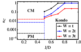
Figure 4: (Color online) Critical MI density $n_{c}$ as function of $J/D$ for graphene ($\varepsilon_{F}=3t$, Dirac point) $L$, $M$, $N$ as in Fig. 1.

V Doniach Phase Diagram of disordered 2DES and Graphene.

We find, that the Kondo phase splits at finite temperature into a Kondo Fermi-liquid (FL) phase, where all MIs are screened, and a Kondo Non-Fermi-liquid (NFL) phase, at $T>T^{*}(n)$, where some MIs remain unscreened and contribute to the magnetic susceptibility with an anomalous temperature dependence, given by,Kettemann et al. (2012)

$$\chi(T)\sim\frac{n}{E_{c}}\frac{2d}{\eta_{2D}}\left(\frac{T}{E_{c}}\right)^{\frac{\eta_{2d}}{2d}-1}{\rm for\,}T>T^{*}(n)>\frac{D}{\xi^{2}}.$$ (7)

The temperature $T^{*}(n)$, plotted schematically in Fig. 5  (blue line), is given by the position of the low $T_{K}$ peak in the distribution $P(T_{K})$, see Fig. 2 c. We note that $J$ may be distributed itself and may add a nonuniversal, material dependent contribution to the distribution of $T_{K}$Langenfeld and Wölfle (1995) and $J_{\rm RKKY}$.

For $n>n_{c}$ there is a succession of phases, starting with the RKKY phase where clusters are formed locally due to the widely distributed RKKY coupling. Anomalous power laws are observed when clusters are broken up successively as temperature is raised. From the log-normal distribution $N(|J_{\rm RKKY}|)$ one obtains for the magnetic susceptibility,

$$\chi(T)T = n_{FM}(T)=\int_{0}^{T}d|J_{\rm RKKY}|N(|J_{\rm RKKY}|)$$ (8)

$$\sim n\exp\Big{[}-\ln^{2}(T/|J_{\rm RKKY}^{0}|)/(2\sigma(W))^{2}\Big{]},$$

where width $\sigma(W)$ increases with disorder strength $W$. Accordingly, the excess specific heat is

$$C(T)=T\frac{dn_{FM}}{dT}\sim\exp\Big{[}-\ln^{2}(T/|J_{\rm RKKY}^{0}|)/(2\sigma(W)^{2}\Big{]}.$$ (9)

The detailed analysis of the quantum phase diagram at higher concentrations $n$ requires to go beyond our present analysis. One expects that at $n>n_{SG}$ a spin-glass phase appears, where the magnetic susceptibility shows a peak at spin glass temperature $T_{SG}$ as studied in Refs. Binder and Young, 1986; Coqblin et al., 2003. Above a critical density $n_{F}$ a phase with long range order may form below a critical temperature $T_{c}(n,J)$.Coqblin et al. (2003); Varma (1976); Magalhaes et al. (2006); Bouzerar et al. (2005)

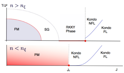
Figure 5: (Color online) Schematic Doniach diagram: temperature $T$ divided by $J^{2}$ versus $J/D$. Vertical dotted line: critical point $J_{c}(n)$ separating RKKY phase from Kondo phase. Blue line: $T^{*}(n)$ separating Kondo FL phase from Kondo NFL phase. For $n<n_{\xi}$ and $J<J_{c}$ a paramagnetic phase (PM) appears.

VI Conclusions and Discussion

We conclude that it is the full distribution function $N(x_{JK})$ of the ratio of the RKKY coupling and the Kondo temperature which determines the magnetic phase diagram of magnetic moments in disordered electron systems, especially at low concentrations. We identified a critical density of magnetic impurities $n_{c}$ below which Kondo wins at all positions in a disordered sample above a critical coupling $J_{c}$, which increases with the disorder amplitude. As a result, the Kondo phase is diminished as the disorder is increased, favoring a phase where the MI spins are coupled. The magnetic susceptibility obeys an anomalous power law behavior, which crosses over as function of $J$ from the Kondo regime where that power is determined by the wide distribution of the Kondo temperature $T_{K}$, to a spin coupled phase where it is governed by the log-normal distribution of $J_{\rm RKKY}$. At low densities and small $J<J_{c}$, we identify a paramagnetic phase. The distribution function of $|J_{\rm RKKY}|/T_{K}$ is expected to determine also the magnetic phase diagram of magnetically doped graphene and the surface of topological insulators with magnetic adatoms, see Fig. 4. This distribution function may also be crucial to explain the anomalous magnetic properties of doped semiconductors in the vicinity of metal-insulator transition,v. Löhneysen (2000) where we expect that $\eta$ is replaced by the universal value $\eta=2(\alpha_{0}-d)$, $d=3$ with the universal multifractality parameter $\alpha_{0}$.

In this work we considered the distribution function of the Kondo temperature of single impurities and the RKKY coupling of pairs of magnetic moments and extracted information on the quantum phase diagram of systems with finite concentrations of MIs. While this approach has its limitations, for example at finite concentration the RKKY coupling can reduce $T_{K}$ as has been already found by Tsay and Klein in the 70s.Tsay and Klein (1973, 1975) However, they concluded that this reduction is minor. More importantly, later work revealed that the Kondo lattice of a finite density of magnetic moments, which is coupled to the conduction electrons, has a coherent low temperature heavy fermion phase, and a Kondo insulator phase at half filling of the magnetic moment levels. More recently, the Kondo lattice in 1 dimension was studied more rigorously (see the review by Tsunetsugu et. alTsunetsugu et al. (1997)), and it was shown that, at least in 1D, the groundstate of this system can not be understood by the mere extension of the single and two-magnetic impurity problem, where the physics is governed by the competition between these two energy scales, the Kondo temperature and the RKKY coupling. However, the higher temperature behavior was found to be still governed by the competition between these two energy scales. Therefore, we expect that the consideration of the reduced problem of two impurity spins, will give important information on the physics of disordered electron systems at finite concentration of magnetic moments, which becomes more meaningful the lower the density and the higher the temperature is. Going beyond the limitations of this approach, one will have to study the disordered Kondo lattice where a finite density of magnetic moments is coupled to the conduction electrons. For a clean Kondo lattice it is known that a coherent low temperature heavy fermion phase, and a Kondo insulator phase at half filling of the magnetic moment levels appears.Coleman (1984); Newns and Read (1987) It remains to see how these low temperature phases are modified by the presence of nonmagnetic disorder.