Stability of three-sublattice order in $S=1$ bilinear-biquadratic Heisenberg Model on anisotropic triangular lattices

Abstract

The $S=1$ bilinear-biquadratic Heisenberg model on anisotropic triangular lattices is investigated by several complementary methods. Our focus is on the stability of the three-sublattice spin nematic state against spatial anisotropy. We find that, deviated from the case of isotropic triangular lattice, quantum fluctuations enhance and the three-sublattice spin nematic order is reduced. In the limit of weakly coupling chains, by mapping the systems to an effective one-dimensional model, we show that the three-sublattice spin nematic order develops at infinitesimal interchain coupling. Our results provide a complete picture for smooth crossover from the triangular-lattice case to both the square-lattice and the one-dimensional limits.

I introduction

Spin nematic states are the states of quantum spin systems in which no spin-dipolar ordering exists, but spin-rotation symmetry is spontaneously broken due to the appearance of spin-quadrupolar order. Penc_Laeuchli Prominent examples for the existence of such spin nematic phases include the spin-1 bilinear-biquadratic (BLBQ) model. Penc_Laeuchli ; Papanicolaou88 Interest in quantum states with spin nematic order has been raised recently by experimental findings in NiGa₂S₄, which is an insulating quantum magnet with spin-1 Ni²⁺ ions living on a triangular lattice. Nakatsujui05 This system is found to be in a gapless ground state without spin-dipolar ordering. It has been suggested that this compound can be considered as a physical realization of the BLBQ model on a triangular lattice and the candidate ground state is characterized by a three-sublattice spin nematic order. Tsunetsugu06 ; Lauchli06 The observed gapless excitation spectrum thus corresponds to the Nambu-Goldstone modes associated with spontaneous breaking of spin-rotation symmetry.

While consensus has been reached for the ground states of the BLBQ model on a triangular lattice, Penc_Laeuchli physics for spatially anisotropic models has not yet been addressed. Here we consider the spin-1 BLBQ model on anisotropic triangular lattices [see Fig. 1(a)] defined by the Hamiltonian,

$$H = J_{1}\sum_{\langle i,j\rangle}\left[\cos\theta\;\mathbf{S}_{i}\cdot\mathbf{S}_{j}+\sin\theta\;(\mathbf{S}_{i}\cdot\mathbf{S}_{j})^{2}\right]$$ (1)

$$+J_{2}\sum_{\langle\langle i,j\rangle\rangle}\left[\cos\theta\;\mathbf{S}_{i}\cdot\mathbf{S}_{j}+\sin\theta\;(\mathbf{S}_{i}\cdot\mathbf{S}_{j})^{2}\right]\;,$$

where $\mathbf{S}_{i}$’s are spin-1 operators. We use the notations $\langle i,j\rangle$ and $\langle\langle i,j\rangle\rangle$ to denote the nearest-neighbour bonds and the bonds along only one of the diagonals, respectively. $J_{1}$ and $J_{2}$ are the coupling strengths on the corresponding bonds. The relative strength of the linear and the biquadratic couplings is parameterized by $\theta$. Here $\alpha\equiv J_{2}/J_{1}$ defines the extent of spatial anisotropy. As the anisotropy $\alpha$ increases from zero, the model changes from the square lattice to the isotropic triangular lattice, and eventually to decoupled chains. We concentrate on the parameter region of $J_{1},\;J_{2}\geq 0$ and $\pi/4\leq\theta<\pi/2$, where the ground states with three-sublattice spin nematic order are expected.

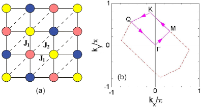
Figure 1: (Color online) (a) Illustration of the anisotropic triangular lattice in a square topology and the schematic representation of three-sublattice spin nematic order. Two groups of interactions, $J_{1}$ and $J_{2}$, are denoted by solid and dashed links, respectively. Here the three mutually orthogonal vectors $\mathbf{d}_{i}$ in the mean-field analysis (see Sec. II.1) are associated with three different colors. (b) Brillouin zone of square lattice. The reduced Brillouin zone for the three-sublattice order is enclosed by dashed lines. The $\mathbf{k}$ path used in Fig. 4 is defined as follows: $\Gamma:(0,0)$, $M:(\pi/3,\pi/3)$, $K:(-\pi/9,7\pi/9)$, and $Q:(-5\pi/9,5\pi/9)$.

The model in Eq. (1) includes several limiting cases, in which the ground states are known:

(i) At $J_{1}=0$, the anisotropic model becomes a set of decoupled one-dimensional (1D) BLBQ spin chains, in which each spin interacts with two neighbors only (i.e., the coordination number $z=2$). For each spin chain with $\pi/4\leq\theta<\pi/2$, the system is found to be in an extended critical phase with soft modes at momenta $k=0$, $\pm 2\pi/3$. Fath91 Away from the SU(3) point ($\theta=\pi/4$), this phase develops dominant antiferro-quadrupolar correlations with a period of three lattice units (i.e., almost “trimerized” ground state). Itoi97 ; Lauchli06_PRB

(ii) At $J_{1}=J_{2}$, the model in Eq. (1) is equivalent to an isotropic triangular-lattice model with $z=6$. The ground state for $\pi/4\leq\theta<\pi/2$ is shown to poss a three-sublattice spin nematic order, Tsunetsugu06 ; Lauchli06 where the nematic directors on the three sublattices $A$, $B$, and $C$ of the triangular lattice are orthogonal to each other (say, along $\hat{x}$, $\hat{y}$, and $\hat{z}$, respectively). The schematic representation of this order is shown in Fig. 1(a).

(iii) At $J_{2}=0$, our model reduces to a square-lattice model with $z=4$. It is established only recently that the ground state for $\pi/4\leq\theta<\pi/2$ develops an unexpected three-sublattice spin nematic order as a consequence of a subtle quantum order-by-disorder mechanism. Toth10 ; Toth12 ; Bauer12

In this paper, the spatially anisotropic BLBQ model in Eq. (1) is investigated. We pay our attention to the effect of spatial anisotropy on the stability of the three-sublattice spin nematic state in this model. Our main results for generic cases of anisotropy are based on the linear flavor-wave (LFW) theory, Penc_Laeuchli ; Papanicolaou88 ; Chubukov90 ; Joshi99 which has been applied to the triangular-lattice as well as the square-lattice cases with success. Tsunetsugu06 ; Lauchli06 ; Toth10 ; Toth12 ; Bauer12 We find that three-sublattice spin nematic order is most robust in the case of isotropic triangular lattice with anisotropy $\alpha\equiv J_{2}/J_{1}=1$. As deviated from this $\alpha=1$ case, quantum fluctuations enhance and the order is reduced. This behavior is reasonable, since the coordination number $z$ is decreased both in the $\alpha\rightarrow 0$ (square-lattice limit) and the $\alpha\rightarrow\infty$ (decoupled-chain limit) cases, and stronger quantum fluctuations are thus allowed. In order to address the validity of the LFW theory, we have performed exact diagonalizations (ED) on lattices of small sizes. By comparing our LFW predictions specialized to finite-size systems with the numerical results, we find that quantum fluctuations obtained by the LFW theory are overestimated, especially in both $\alpha\rightarrow 0$ and $\alpha\rightarrow\infty$ limits. Thus the stability region of the three-sublattice state could be larger than the LFW predictions. Since previous numerical investigations, Toth10 ; Toth12 ; Bauer12 have shown nonzero order in the square-lattice case at $\theta=\pi/4$, one may expect that the three-sublattice order could persist down to the $\alpha=0$ limit in the whole region of $\pi/4\leq\theta<\pi/2$. In the opposite large-$\alpha$ limit, the status is much less clear. Because there is no true long-range order at the decoupled-chain limit ($J_{1}/J_{2}=1/\alpha=0$), Fath91 ; Itoi97 ; Lauchli06_PRB an interesting issue is whether a nonzero interchain coupling is necessary or not for the appearance of two-dimensional (2D) three-sublattice order. By mapping from the system of weakly coupled chains ($J_{1}/J_{2}\ll 1$) to an effective 1D model, we show that the critical value of interchain coupling is $(J_{1}/J_{2})_{c}=0$ for all $\pi/4<\theta<\pi/2$. In other words, the transition from the 2D three-sublattice phase to the 1D “trimerized” critical phase Fath91 ; Itoi97 ; Lauchli06_PRB should occur at infinite $\alpha$.

The rest part of the paper is organized as follows. Generic cases of anisotropy are discussed in Sec. II, where details of the LFW analysis are presented in Sec. II A and the comparison between the finite-size LFW and the ED results is made in Sec. II B. The case in the decoupled-chain limit is explored in Sec. III through field-theoretical approach as well as ED calculations. The last section is devoted to our conclusions.

II Generic anisotropy

II.1 linear flavor-wave analysis

The LFW theory starts from representing the model in Eq. (1) in terms of three-flavor Schwinger bosons $a_{i,\alpha}$ under the local constraint $\sum_{\alpha}a_{i,\alpha}^{\dagger}a_{i,\alpha}=1$. Penc_Laeuchli ; Papanicolaou88 ; Chubukov90 ; Joshi99 ; Tsunetsugu06 ; Lauchli06 ; Toth10 ; Toth12 ; Bauer12 The Schwinger bosons $a_{i,\alpha}^{\dagger}$ (with $\alpha=x$, $y$, $z$) create three time-reversal-invariant local basis states, $|x\rangle=\frac{i}{\sqrt{2}}(|s_{z}=1\rangle-|s_{z}=-1\rangle)$, $|y\rangle=\frac{1}{\sqrt{2}}(|s_{z}=1\rangle+|s_{z}=-1\rangle)$, and $|z\rangle=-i\;|s_{z}=0\rangle$. In terms of these bosons, the spin operators become $S_{i}^{\alpha}=-i\sum_{\beta,\gamma}\epsilon_{\alpha\beta\gamma}a_{i,\beta}^{\dagger}a_{i,\gamma}$. We denote $\mathbf{d}_{i}$ as the local ordering vector and let $\{\mathbf{d}_{i},\mathbf{e}_{i},\mathbf{f}_{i}\}$ forming a local orthonormal basis. A generic local quantum state can be represented by the linear combination of the three basis states $\{\left|\mathbf{d}_{i}\right>,\left|\mathbf{e}_{i}\right>,\left|\mathbf{f}_{i}\right>\}$. Let $a_{i}^{\dagger}$, $b_{i}^{\dagger}$ and $c_{i}^{\dagger}$ representing the Schwinger boson operators which create the local states $\{\left|\mathbf{d}_{i}\right>,\left|\mathbf{e}_{i}\right>,\left|\mathbf{f}_{i}\right>\}$ out of the Schwinger boson vacuum. They are related to the operators $a_{i,\alpha}$ through the relation $a_{i,\alpha}=d_{i,\alpha}\,a_{i}+e_{i,\alpha}\,b_{i}+f_{i,\alpha}\,c_{i}$. Within the LFW analysis, we solve the local constraint $a_{i}^{\dagger}a_{i}+b_{i}^{\dagger}b_{i}+c_{i}^{\dagger}c_{i}=1$ by replacing $a_{i}=\sqrt{1-b_{i}^{\dagger}b_{i}-c_{i}^{\dagger}c_{i}}\approx 1$ and thus $a_{i,\alpha}\approx d_{i,\alpha}+e_{i,\alpha}\,b_{i}+f_{i,\alpha}\,c_{i}$. It has be shown that, for $\pi/4\leq\theta<\pi/2$, the mean-field energy of the nearest-neighbor bond is minimized when the $\mathbf{d}_{i}$ vectors are mutually orthogonal. Penc_Laeuchli In the case of isotropic triangular lattice, these $\mathbf{d}_{i}$ vectors are given by the unit vectors along the $x$, $y$, and $z$ directions on the three sublattices [see Fig. 1(a)]. Employing this mean-field condition and the approximate expression for $a_{\alpha,i}$, the model in Eq. (1) reduces to the following quadratic LFW Hamiltonian (up to a constant term),

$$H_{\textrm{LFW}}=2\sum_{\mathbf{k}} \left[\epsilon_{0}(b_{\mathbf{k}}^{\dagger}b_{\mathbf{k}}+c_{\mathbf{k}}^{\dagger}c_{\mathbf{k}})+(\Delta_{\mathbf{k}}^{*}b_{\mathbf{k}}c_{-\mathbf{k}}+\textrm{h.c.})\right.$$

$$\left.+(\phi_{\mathbf{k}}b_{\mathbf{k}}^{\dagger}c_{\mathbf{k}}+\textrm{h.c.})\right]\,.$$ (2)

Here the values of $\mathbf{k}$ run over the first Brillouin zone of the square lattice and

$$\epsilon_{0} = (J_{1}+\frac{J_{2}}{2})\sin\theta\;,$$

$$\Delta_{\mathbf{k}} = \frac{\cos\theta}{2}\left[J_{1}(e^{ik_{x}}+e^{ik_{y}})+J_{2}\;e^{-i(k_{x}+k_{y})}\right]\;,$$ (3)

$$\phi_{\mathbf{k}} = (\tan\theta-1)\Delta_{\mathbf{k}}\;.$$

For $\mathbf{k}\neq 0,\pm\mathbf{k}_{0}$ with $\mathbf{k}_{0}=(2\pi/3,2\pi/3)$, the resulting quadratic bosonic Hamiltonian can be diagonalized by the Boguliubov transformation, and the corresponding excitation spectrums are given by

$$\omega_{1,2}(\mathbf{k}) =2\left[\epsilon_{0}^{2}+\left|\phi_{\mathbf{k}}\right|^{2}-\left|\Delta_{\mathbf{k}}\right|^{2}\right.$$

$$\left.\pm\sqrt{2\left|\phi_{\mathbf{k}}\right|^{2}(2\epsilon_{0}^{2}-\left|\Delta_{\mathbf{k}}\right|^{2})+(\phi_{\mathbf{k}}^{*})^{2}\Delta_{\mathbf{k}}^{2}+(\Delta_{\mathbf{k}}^{*})^{2}\phi_{\mathbf{k}}^{2}}\right]^{1/2}\,.$$ (4)

The modes for $\mathbf{k}=0,\pm\mathbf{k}_{0}$ cannot be diagonalized in this way, because the Boguliubov transformation becomes singular here. As discussed in the finite-size spin-wave theory for spin-$1/2$ Heisenberg model, Zhong93 ; Trumper00 these singular modes have no contribution to the ground-state energy, while removal of these modes is required in the computation of order parameter.

Some general features of the LFW excitation spectrums are described below. At the SU(3) point of $\theta=\pi/4$, we have $\phi_{\mathbf{k}}=0$ and thus these two excitation modes become degenerate in energy. Away from this special point, $\omega_{1}(\mathbf{k})$ gives a gapped mode, while $\omega_{2}(\mathbf{k})$ is gapless and has nodes at $\mathbf{k}=0,\pm\mathbf{k}_{0}$. We remind that the primitive unit cell of three-sublattice states contains three lattice sites as its basis and therefore its size becomes three times larger. As a consequence, the original Brillouin zone of square lattice behaves as an extended Brillouin zone [as shown in Fig. 1(b)], such that each branch of excitations in Eq. (4) becomes three-fold degenerate within the original Brillouin zone. As a simple check for our derivations, we point out that the obtained dispersions at $J_{2}=0$ do reduce to those in Ref. Toth10, for the square-lattice case. For the case of isotropic triangular lattice ($J_{1}=J_{2}$), they are equivalent to the results in Ref. Tsunetsugu06, .

To determine the stability region of the three-sublattice states, a suitable order parameter should be measured. In the spin nematic state, spin rotational symmetry is spontaneously broken, though time reversal symmetry is preserved. In such a state, average magnetic moment must vanish ($\langle\mathbf{S}\rangle=0$). Nevertheless, quadrupole order can appear, which is characterized by a nonzero expectation value of the symmetric and traceless rank-2 tensor operator

$${\cal Q}^{\alpha\beta}_{i}=\frac{1}{2}\left(S^{\alpha}_{i}S^{\beta}_{i}+S^{\beta}_{i}S^{\alpha}_{i}\right)-\frac{2}{3}\delta^{\alpha\beta}\;.$$ (5)

Here $S^{\alpha}_{i}$ is the $\alpha$ component of spin-1 operator at site $i$ and $\delta^{\alpha\beta}$ is the Kroneker delta symbol. In terms of the local ordering vector $\mathbf{d}_{i}$, the expectation value of this quadrupole operator can be written as

$$\langle{\cal Q}_{i}^{\alpha\beta}\rangle=-q\left(d_{i}^{\alpha}d_{i}^{\beta}-\frac{1}{3}\delta^{\alpha\beta}\right)\;,$$ (6)

where the constant value of $q$ describes the magnitude of the quadrupolar ordering. For both cases of the triangular and the square lattices, Tsunetsugu06 ; Toth10 the $\mathbf{d}_{i}$ vectors of the three-sublattice states point along three orthogonal directions in three different sublattices, as shown in Fig. 1(a). From Eqs. (5) and (6), we have (from now on, summation is implied over the repeated Greek indices)

$$q=-\frac{3}{2}\langle{\cal Q}_{i}^{\alpha\beta}\rangle d_{i}^{\alpha}d_{i}^{\beta}=1-\frac{3}{2}\langle(\mathbf{S}_{i}\cdot\mathbf{d}_{i})^{2}\rangle\;.$$ (7)

At classical level, $q=1$ because $(\mathbf{S}_{i}\cdot\mathbf{d}_{i})|\mathbf{d}_{i}\rangle=0$.

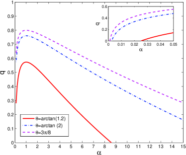
Figure 2: (Color online) Effect of anisotropy $\alpha=J_{2}/J_{1}$ on the quadrupole order parameter $q$ within the LFW theory for various values of $\theta$. The inset shows the details around the region of $\alpha=0$.

Within the LFW theory, $q$ can be expressed by

$$q=1-\frac{3}{2}\left<\Delta n_{a}\right>$$ (8)

with

$$\left<\Delta n_{a}\right>=1-\frac{1}{N}\sum_{i}\left<a_{i}^{\dagger}a_{i}\right>=\frac{1}{N}\sum_{i}\left<b_{i}^{\dagger}b_{i}+c_{i}^{\dagger}c_{i}\right>$$ (9)

being the deviation of the number density for the Schwinger boson $a_{i}$ from its classical value of one. Here $N$ is the total number of lattice sites. We note that this expression of $q$ is nothing but the local moment defined in Eq. (24) of Ref. Bauer12, . From this expression, it is obvious that the quantum correction for $q$ comes from the non-vanishing contribution of $\left<\Delta n_{a}\right>$. When $\left<\Delta n_{a}\right>$ increases to $2/3$, $q$ vanishes. This gives a phase transition out of the three-sublattice states within the LFW theory. The explicit expression of $\left<\Delta n_{a}\right>$ is given by

$$\left<\Delta n_{a}\right>=\frac{1}{N}\sum_{\mathbf{k}\neq 0,\pm\mathbf{k}_{0}}\left(\frac{\epsilon_{0}+\left|\phi_{\mathbf{k}}\right|}{\omega_{1}(\mathbf{k})}+\frac{\epsilon_{0}-\left|\phi_{\mathbf{k}}\right|}{\omega_{2}(\mathbf{k})}-1\right)\;.$$ (10)

Here the singular modes at $\mathbf{k}=0,\pm\mathbf{k}_{0}$ are excluded from this summation. Note that, for the case of square lattice ($J_{2}=0$) and at the SU(3) point ($\theta=\pi/4$), Eq. (10) reduces to $\left<\Delta n_{a}\right>=\frac{1}{N}\sum_{\mathbf{k}\neq 0,\pm\mathbf{k}_{0}}\left(\frac{1}{\sqrt{1-\left|\gamma_{\mathbf{k}}\right|^{2}}}-1\right)$ with $\gamma_{\mathbf{k}}=\cos[(k_{x}-k_{y})/2]$, and reproduces the previous result (see Eq. (22) of Ref. Bauer12, ). The general behavior of the order parameter $q$ as functions of $\alpha$ for distinct values of $\theta$ is shown in Fig. 2. It is seen clearly that the three-sublattice nematic order is most robust at $\alpha=1$. Far away from this point of isotropic triangular lattice, quantum fluctuations arising from the flavor-wave excitations become more stronger, and they destroy eventually the quadrupolar ordering in both limits of $\alpha\rightarrow 0$ and $\alpha\rightarrow\infty$. Exploiting Eqs. (8) and (10) and employing the condition $q=0$ as the criterion for the transitions out of the three-sublattice states, we can establish the phase boundaries of the three-sublattice states as shown in Fig. 3. We find that, in general, the lower transition points are nonzero and the upper ones are large but finite. The stability region of the three-sublattice order is largely reduced as $\theta$ approaches the SU(3) point ($\theta=\pi/4$). It implies that there exist more low-lying excitations and thus larger quantum fluctuations as $\theta$ gets closer to $\pi/4$.

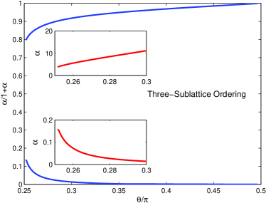
Figure 3: (Color online) Phase diagram for the spatially anisotropic $S=1$ BLBQ model in Eq. (1) determined by the LFW theory. The insets show the details of two phase boundaries around $\theta=\pi/4$.

As seen from the expression of Eq. (10), the gapless mode $\omega_{2}(\mathbf{k})$ should make a dominant contribution in reducing the three-sublattice order. To have a better understanding of the enhancement of quantum fluctuations both in the square-lattice limit ($\alpha\to 0$) and the quasi-1D limit ($\alpha\gg 1$), it is instructive to examine the softening behavior of this excitation mode more closely. The flavor-wave dispersions of the gapless branch $\omega_{2}(\mathbf{k})$ along the path defined in Fig. 1(b) for various values of anisotropy $\alpha=J_{2}/J_{1}$ are shown in Fig. 4. It can be seen that, as system approaches the square-lattice limit ($\alpha\to 0$), the flavor-wave velocity at the $\Gamma$ point (defined by the slope of the dispersion relation) decreases to zero. Therefore, the excitation modes along the $\Gamma$-$M$ line (i.e., line of $k_{x}=k_{y}$) become zero-energy modes eventually. On the other hand, in the limit of decoupled chains ($\alpha\to\infty$), the excitation energies in the whole Brillouin zone are softened. Within the LFW theory, the disappearance of three-sublattice order in both limits of $\alpha\to 0$ and $\alpha\to\infty$ can be explained by such softening in energy.

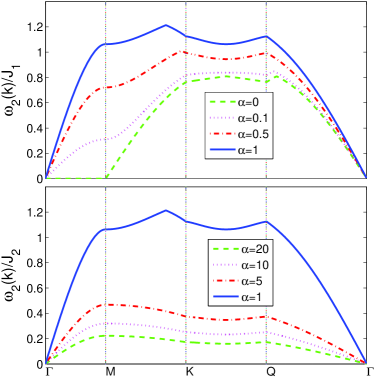
Figure 4: (Color online) Dispersion relation of gapless branch $\omega_{2}(\mathbf{k})$ of the flavor-wave excitation for different anisotropy parameters $\alpha=J_{2}/J_{1}$ at $\theta=0.3\pi$. Note that energies are measured in unit of $J_{1}$ for $\alpha<1$ (upper panel), while they are measured in unit of $J_{2}$ for $\alpha>1$ (lower panel).

Near the node, say, at $\mathbf{k}=0$, analytic expressions can be derived. By expanding $\Delta_{\mathbf{k}}$ in Eq. (II.1) near $\mathbf{k}=0$, we can show that the gapless flavor-wave mode behaves as $\omega_{2}(\mathbf{k})/J_{1}\approx\sqrt{c_{+}^{2}k_{+}^{2}+c_{-}^{2}k_{-}^{2}}$ with $k_{\pm}=\frac{1}{\sqrt{2}}(k_{x}\pm k_{y})$, $c_{+}=\frac{3}{\sqrt{2}}\sqrt{\sin(2\theta)\alpha}$, and $c_{-}=\frac{1}{\sqrt{2}}\sqrt{\sin(2\theta)(\alpha+2)}$. For $\alpha\to 0$, we have $c_{+}\to 0$ while $c_{-}$ remaining finite. The outcome of $c_{+}=0$ for $\alpha=0$ gives a nodal line in the excitation spectrum along the $k_{x}=k_{y}$ direction (i.e., $\Gamma$-$M$ line), as observed in Fig. 4. Within the LFW theory, these soft modes play a significant role in the destruction of the nematic order in the square-lattice limit, as noticed in the previous investigations. Toth10 ; Bauer12 On the other hand, in the extreme anisotropic quasi-1D limit ($J_{1}\to 0$ or $\alpha\to\infty$), we have $c_{-}/c_{+}=1/3$ for all values of $\theta$. That is, this ratio of the flavor-wave velocities does not goes to zero in the quasi-1D limit. Instead, the whole spectrum, in unit of the diagonal coupling $J_{2}$, becomes nearly flat in the entire Brillouin zone, as seen from Fig. 4. Therefore, the associated quantum fluctuations become more and more significant and finally the 2D nematic order ceases to exist for $\alpha$ being large enough. We stress that the mode softening of the flavor-wave excitations in the quasi-1D limit is quite different from what one got for the spin-wave excitations in spatially anisotropic spin-$1/2$ antiferromagnetic Heisenberg models on either triangular Merino99 or square lattices. Sakai89 ; Affleck94 In these spin-$1/2$ cases, one can show that, as the interchain couplings approach zero, only the spin-wave velocity $c_{\perp}$ for the excitation transverse to the chains will vanish, but the spin-wave velocity $c_{\parallel}$ for the excitation along the chains will remain finite. Thus the whole spectrum, in unit of the intrachain coupling, never becomes nearly flat in the whole Brillouin zone, and the ratio of these two spin-wave velocities $c_{\perp}/c_{\parallel}$ does go to zero in the quasi-1D limit.

We remind that the LFW analysis is valid only when quantum fluctuations are weak (i.e., only when $\langle b_{i}^{\dagger}b_{i}\rangle+\langle c_{i}^{\dagger}c_{i}\rangle\ll 1$) because the local constraint, $a_{i}^{\dagger}a_{i}+b_{i}^{\dagger}b_{i}+c_{i}^{\dagger}c_{i}=1$, is considered only approximatively. Therefore, we should be cautious with the LFW results about the phase boundaries shown in Fig. 3, since large quantum fluctuations are expected near the transition points. To examine the validity of the LFW predictions, comparison with exact results is necessary.

II.2 exact diagonalizetion

In this subsection, we perform ED calculations for the Hamiltonian in Eq. (1) on small clusters and compare the results with those obtained by the LFW analysis on the same clusters.

We remind that there exist subtleties in making careful comparison of order parameter between symmetry-breaking solutions (say, LFW results) and symmetry-nonbreaking ones (say, ED findings). Such an observation has been put forward in Ref. Bernu94, in concern with magnetic ordering in spin-$1/2$ Heisenberg antiferromagnets on a triangular lattice. To uncover the long-range order on lattices of small sizes, a proper quantity has to be measured in ED calculations. Here the squared quadrupole moment $\mathcal{Q}^{2}$ in a given sublattice (say, $A$ sublattice) is considered,

$$\mathcal{Q}^{2}\equiv\left\langle\left(\sum_{j\in A}\mathcal{Q}^{\alpha\beta}_{j}\right)^{2}\right\rangle=\sum_{i,j\in A}\left\langle\mathcal{Q}^{\alpha\beta}_{i}\mathcal{Q}^{\alpha\beta}_{j}\right\rangle\;.$$ (11)

As mentioned before, the Einstein summation convention for the repeated Greek indices is assumed. The signature of three-sublattice order will be manifested as a macroscopic value of $\mathcal{Q}$. To obtain a order parameter that is normalized to 1 in the absence of quantum fluctuations, the sublattice quadrupole moment $\mathcal{Q}$ should be divided by a size-dependent normalization factor. For deriving the correct normalization factor, it should be kept in mind that the sublattice quadrupole moment cannot be treated as a classical quantity. For example, it can be shown that there exists an exact operator identity: $\mathcal{Q}^{\alpha\beta}_{i}\mathcal{Q}^{\alpha\beta}_{i}=5/3$ on a given site $i$. On the other hand, when $i$ and $j$ denote different sites of the same sublattice, $\left\langle\mathcal{Q}^{\alpha\beta}_{i}\mathcal{Q}^{\alpha\beta}_{j}\right\rangle=2/3$ for fully aligned classical ordered state. From these observations, the maximum quantum value of $\mathcal{Q}^{2}$ can be shown to be $(2N^{2}/27)(1+9/2N)$ for systems of $N$ sites. Thus a valid definition of the order parameter would be

$$q=\sqrt{\frac{27\mathcal{Q}^{2}}{2N^{2}(1+\frac{9}{2N})}}\;.$$ (12)

Now $q$ saturates at one in the classical state and should be decreased by quantum fluctuations in the quantum ground state. We stress that, for careful comparison between the ED and the LFW results for small values of $N$, it is important to use the correct normalization factor in the definition of the order parameter $q$.

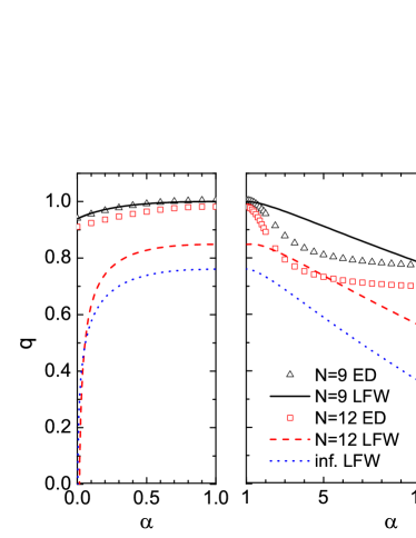
Figure 5: (Color online) Comparison of order parameter $q$ between the ED and the LFW results for different lattice sites as anisotropy $\alpha$ ia varied. Here, $\theta=\arctan(2)$. The ED data are obtained on lattices with sites $N=9$ (triangles) and $N=12$ (squares). The LFW results of the corresponding sizes are shown by solid and dashed lines, respectively. The lowest curve refers to the infinite-size LFW results (dotted line).

The comparison between the ED and the LFW results is shown in Fig. 5 for $\theta=\arctan(2)$. The ED data are calculated by using Eqs. (11) and (12). On the other hand, the LFW results for systems of finite sizes are obtained from Eqs. (8) and (10) by summing the momenta (except $\mathbf{k}=0$, $\pm\mathbf{k}_{0}$) determined by the clusters in ED calculations. We find that, around the isotropic point ($\alpha=1$), two sets of results do not differ by large amounts. Good agreement can persist even down to the $\alpha=0$ limit for the special case of $N=9$. This indicates that the LFW theory does in general provide good approximation around $\alpha=1$. However, serious reduction in the LFW results of $q$ as compared to the ED ones is observed both when $\alpha\ll 1$ and $\alpha\gg 1$. This implies that quantum fluctuations are significantly overestimated in the LFW analysis in both of the square-lattice and the quasi-1D limits. In other words, the softening of the flavor-wave excitations in both limits (see Fig. 4) should be exaggerated. Thus one has to go beyond the LFW approximation to find improvements on the excitation spectrums. According to previous numerical investigations, Toth10 ; Toth12 ; Bauer12 where nonzero order was reported in the square-lattice case at $\theta=\pi/4$, the lower phase boundary obtained within the LFW theory (see Fig. 3) may be illusive. Instead, the three-sublattice order may persist down to the $\alpha=0$ limit in the whole region of $\pi/4\leq\theta<\pi/2$.

The above comparison suggests as well that the upper phase boundary may take much larger values than the ones estimated by the LFW theory. To achieve the true values of the transition points in the large $\alpha$ limit, it is instructive to analyze the model from its quasi-1D limit. Because there is no true long-range order in strictly 1D models, our main concern is to show whether a nonzero interchain coupling is necessary or not to establish the 2D order. This is what we shall do in the next section.

III weakly-coupled-chain limit

When $J_{1}\ll J_{2}$, the system described by Eq. (1) reduces to weakly coupled 1D chains with intrachain coupling strength $J_{2}$ and weak interchain coupling strength $J_{1}$. Taking advantage of conventional mean-field treatment for the interchain coupling, Sakai89 ; Affleck94 ; Scalapino75 ; Schulz96 our quasi-1D systems can be transformed into effective single-chain problems.

The desired effective single-chain model can be derived in the following way. Using the definition of the quadrupole operator in Eq. (5), the part of Hamiltonian with the interchain coupling $J_{1}$ can be rewritten as

$$H_{1}=J_{1}(\cos\theta-\frac{\sin\theta}{2})\sum_{\langle ij\rangle}\mathbf{S}_{i}\cdot\mathbf{S}_{j}+J_{1}\sin\theta\sum_{\langle ij\rangle}{\cal Q}^{\alpha\beta}_{i}{\cal Q}^{\alpha\beta}_{j}$$ (13)

by dropping some constant terms. Again, the repeated Greek indices imply the Einstein summation convention. Assuming the three-sublattice quadrupolar ordering, in which $\langle\mathbf{S}_{j}\rangle=0$ but $\langle{\cal Q}_{j}^{\alpha\beta}\rangle$ is nonzero, $H_{1}$ can be approximated by an on-site Hamiltonian,

$$\tilde{H}_{1}=\sum_{n}{\cal Q}_{n}^{\alpha\beta}\left[J_{1}\sin\theta\sum_{m}\langle{\cal Q}_{n+m}^{\alpha\beta}\rangle\right]\;,$$ (14)

where $m$ runs over all neighbors on the $J_{1}$ bonds for the $n$-th site along a given single chain. Substituting suitable mean-field expression for $\langle{\cal Q}_{n+m}^{\alpha\beta}\rangle$, an effective 1D Hamiltonian for the model in Eq. (1) can be written as

$$H_{\textrm{eff}}=J_{2}\sum_{n}\left[\cos\theta\;\mathbf{S}_{n}\cdot\mathbf{S}_{n+1}+\sin\theta\;(\mathbf{S}_{n}\cdot\mathbf{S}_{n+1})^{2}\right]+\tilde{H}_{1}\;.$$ (15)

This describes a 1D BLBQ chain in a self-consistent external field triggering three-sublattice quadrupolar ordering. For convenience, we set $J_{2}\equiv 1$ as the energy unit in this section. We note that the self-consistent field is proportional to $J_{1}\sin\theta$. It is thus expected that, for a given anisotropy (i.e., for a fixed value of $J_{1}$), the resulting order will be stronger as $\theta$ gets closer to $\pi/2$. This observation is consistent with our LFW results, where the stability region of the three-sublattice state is pushed toward larger $\alpha=J_{2}/J_{1}$ as $\theta\to\pi/2$.

In the following, both analytical and numerical techniques are exploited to determine the critical interchain coupling $J_{1,c}$ for the emergence of 2D three-sublattice order.

III.1 scaling analysis

Employing the mean-field expression of $\langle{\cal Q}_{j}^{\alpha\beta}\rangle$ in Eq. (6), the on-site part of Eq. (14) for the effective 1D Hamiltonian becomes

$$\tilde{H}_{1}=h\sum_{n}\left[1-\frac{3}{2}(\mathbf{S}_{n}\cdot\mathbf{d}_{n})^{2}\right]\;,$$ (16)

where the self-consistent field conjugate to the operator for the order parameter $q$ in Eq. (7) is defined by $h\equiv(4/3)qJ_{1}\sin\theta$.

For $J_{1}\ll 1$, the effective 1D Hamiltonian in Eq. (15) can be considered as a 1D BLBQ model in a weak external field $h$. Thus it should be valid to treat the effect of $h$ as a perturbation. It is known from Ref. Itoi97, that, near $\theta=\pi/4$, the 1D BLBQ spin chain can be described by an SU(3)₁ Wess-Zumino-Witten conformal field theory perturbed by some marginally irrelevant current-current interactions. To see whether the three-sublattice order can be induced by vanishing self-consistent field $h$ or not, we need only to calculate the scaling dimension $\Delta_{h}$ of the corresponding operator in the on-site term and then determine its relevancy. If $\Delta_{h}<2$, the on-site term provides a relevant perturbation and thus the three-sublattice order will be induced by an infinitesimal $h$. Otherwise, the on-site term becomes irrelevant and the three-sublattice order can be established only when $h$ exceeds a nonzero critical field $h_{c}$. In this latter case, we need to determine $h_{c}$ numerically by solving this model explicitly.

In terms of the field-theoretical variables discussed in Ref. Itoi97, , the operator in the on-site term of Eq. (16) takes the form of the primary fields of an SU($\nu$) Wess-Zumino-Witten model for $\nu=3$. That is, the scaling dimension $\Delta_{h}$ of our operator is nothing but that of those primary fields, which is equal to $1-1/\nu=2/3$ according to the analysis in Ref. Itoi97, . Because of $\Delta_{h}<2$, the perturbation caused by the self-consistent field is strongly relevant. Since the above scaling argument is essentially independent of the value of $\theta$, we claim that $h_{c}=0$ and thus $J_{1,c}=0$ for $\pi/4<\theta<\pi/2$, even though the field theory in Ref. Itoi97, is derived for $\theta$ close to $\pi/4$. This implies that, for original quasi-1D anisotropic BLBQ model, true phase transitions out of the three-sublattice states actually occur at infinite $\alpha$, rather than at large but finite $\alpha_{c}$ as obtained in the LFW analysis.

We can go one step further to establish a nonperturbative relation between the order parameter $q$ and the weak interchain couplings $J_{1}$ by making use of the field-theoretic approach. According to the standard scaling argument, Cardy the order parameter $q$ induced by the perturbation of self-consistent field $h$ scales as $q\propto h^{\Delta_{h}/(2-\Delta_{h})}$. Combined with the self-consistency relation, $h=(4/3)qJ_{1}\sin\theta$, we get $q\propto(J_{1}\sin\theta)^{\Delta_{h}/[2(1-\Delta_{h})]}$. Since $\Delta_{h}=2/3$, we conclude that $q\propto J_{1}\sin\theta$. Interestingly, this result coincides with the one that is expected naively from the perturbation theory for original $H_{1}$ without taking mean-field approximation. This seems to indicate that it is possible to study this model in its quasi-1D limit directly from perturbation theory for $H_{1}$. Instead of pursuing along this direction, we shall determine the phase boundary by the numerical ED method below.

III.2 exact diagonalization

In this subsection, the critical values of the interchain coupling $J_{1}$ are estimated by the ED method. Here we follow the treatment in Ref. Sakai89, for quasi-1D Heisenberg antiferromagnets. Our ED results provide numerical evidences in supporting the above conclusions based on scaling arguments.

For the sake of ED calculations, we assume here that only the $zz$ component of the expectation value $\langle{\cal Q}_{j}^{\alpha\beta}\rangle$ is nonzero. Thus the effective 1D Hamiltonian in Eq. (15) has still spin-rotation symmetry in the $z$ direction and the total $z$-component spin remains a conserved quantity. This reduces much computational effort and thus calculations for systems of large sizes become available. In consistent with Eq. (6), the explicit form of $\langle{\cal Q}_{j}^{\alpha\beta}\rangle$ is taken to be $\langle{\cal Q}_{j}^{zz}\rangle=\langle(S^{z}_{j})^{2}\rangle-\frac{2}{3}=-\frac{2}{3}q\cos(\mathbf{Q}\cdot\mathbf{r}_{j})$. Substituting the present mean-field solution to Eq. (14), the on-site part of the effective 1D Hamiltonian becomes

$$\tilde{H}_{1}=h\sum_{n}\cos(\frac{4\pi}{3}n)(\mathbf{S}^{z}_{n})^{2}\;.$$ (17)

Here the self-consistent field is again given by $h\equiv(4/3)qJ_{1}\sin\theta$.

By taking $h$ as a free parameter, we diagonalize numerically the effective single-chain model up to system length $L=18$. For the present single-chain problem, the order parameter for spin quadrupole ordering becomes

$$q=-\frac{3}{L}\sum_{n}e^{i\frac{4\pi}{3}n}\langle{\cal Q}_{n}^{zz}\rangle\;.$$ (18)

This expression is compatible with the form of 2D order parameter used in this subsection. The results of $q$ as function of $h$ for several $\theta$’s with $L=18$ are presented in Fig. 6(a). The susceptibility $\chi\equiv(\partial q/\partial h)|_{h=0}$ can then be evaluated from the slope of the linear fit as shown in the inset of this figure. Within the present mean-field approach, to have a nonzero solution of $q$, the slope $\chi$ of the tangent line around $h=0$ must be larger than that of the straight line, $q=h/[(4/3)J_{1}\sin\theta]$, given by the self-consistent relation. That is, long-range order appears only when $\chi\geq 1/[(4/3)J_{1}\sin\theta]$. This requirement leads to a critical value $J_{1,c}$ of the interchain coupling for a given length $L$,

$$J_{1,c}=\frac{1}{(4/3)\chi\sin\theta}\;.$$ (19)

The size dependence of $J_{1,c}$ for various $\theta$’s is shown in Fig. 6(b). As seen from this figure, size dependence of $J_{1,c}$ is more prominent as $\theta$ gets closer to $\pi/4$. This reflects the fact that quantum fluctuations for the 1D systems become larger as $\theta$ approaches to the SU(3) point, where more low-energy excitations appear. Except for the case of $\theta=0.3\pi$, in which size effect may be profound, a smooth extrapolation of $J_{1,c}$ to zero in the thermodynamic limit is found for all $\theta$’s. This indicates that the 2D three-sublattice order will emerge for infinitesimal $J_{1}$ within the whole region of $\pi/4<\theta<\pi/2$. In other words, the phase transitions out of the three-sublattice states actually occur at infinite $\alpha$ for original 2D anisotropic BLBQ model. Thus our ED results lend strong support on the conclusions based on the scaling arguments discussed in the previous subsection.

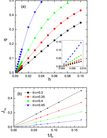
Figure 6: (Color online) (a) Order parameter $q$ as function of self-consistent field $h$ for various $\theta$’s with $L=18$. Lines are guide to eyes. Inset: linear fit around $h=0$ region. (b) Critical value $J_{1,c}$ of the interchain coupling as function of $1/L$. Lines show the extrapolations in the thermodynamic limit by using data for the largest two sizes (i.e., $L=15$ and 18).

IV Conclusions

To summarize, we elaborate the effect of spatial anisotropy $\alpha$ on the stability of the three-sublattice spin nematic state in the model of Eq. (1) through various analytic as well as numerical approaches. We conclude that the three-sublattice state is stable for all $0\leq\alpha<\infty$ within the whole region of $\pi/4<\theta<\pi/2$. Our analysis thus gives a complete picture for smooth crossover from the triangular-lattice case to both the square-lattice and the 1D-chain limits as the anisotropy $\alpha$ is varied. Moreover, our work provides some insights on the validity of the LFW theory. Basically, the strength of the stability for the considered order can be understood within the simple LFW theory. Nevertheless, the predicted phase boundaries and the excitation spectrums is merely suggestive, especially in both of the $\alpha=0$ and $\alpha\to\infty$ limits. Because the local constraints are released in the LFW analysis, it is interesting to see if great improvement can be obtained through other approaches (say, the variational Monte Carlo method), in which these constraints are taken into account rigorously. Such discussions go beyond the scope of the present work and deserve further investigations.

- (1) For a recent review, see K. Penc and A. M. Läuchli, in Introduction to Highly Frustrated Magnetism, Vol. 164 of Springer Series in Solid-State Sciences, edited by C. Lacroix, P. Mendels and F. Mila (Springer, New York, 2011), pp. 331–360.
- (2) N. Papanicolaou, Nucl. Phys. B 305, 367 (1988).
- (3) S. Nakatsuji, Y. Nambu, H. Tonomura, O. Sakai, S. Jonas, C. Broholm, H. Tsunetsugu, Y. Qiu, and Y. Maeno, Science 309, 1697 (2005).
- (4) H. Tsunetsugu and M. Arikawa, J. Phys. Soc. Jap. 75, 083701 (2006).
- (5) A. Läuchli, F. Mila, and K. Penc, Phys. Rev. Lett. 97, 087205 (2006).
- (6) G. Fáth and J. Sólyom, Phys. Rev. B 44, 11836 (1991).
- (7) C. Itoi and M. Kato, Phys. Rev. B 55, 8295 (1997).
- (8) A. Läuchli, G. Schmid, and S. Trebst, Phys. Rev. B 74, 144426 (2006).
- (9) T. A. Tóth, A. M. Läuchli, F. Mila, and K. Penc, Phys. Rev. Lett. 105, 265301 (2010).
- (10) T. A. Tóth, A. M. Läuchli, F. Mila, and K. Penc, Phys. Rev. B 85, 140403(R) (2012).
- (11) B. Bauer, P. Corboz, A. M. Läuchli, L. Messio, K. Penc, M. Troyer, and F. Mila, Phys. Rev. B 85, 125116 (2012).
- (12) A. Chubukov, J. Phys. Condens. Matter 2, 1593 (1990).
- (13) A. Joshi, M. Ma, F. Mila, D.N. Shi, and F.C. Zhang, Phys. Rev. B 60, 6584 (1999).
- (14) Q. F. Zhong and S. Sorella, Europhys. Lett. 21, 629 (1993).
- (15) A. E. Trumper, L. Capriotti, and S. Sorella, Phys. Rev. B 61, 11 529 (2000).
- (16) J. Merino, R. H. Mckenzie, J. B. Marston, and C. H. Chung, J. Phys.: Condens. Matter 11, 2965 (1999).
- (17) T. Sakai and M. Takahashi, J. Phys. Soc. Jpn. 58, 3131 (1989).
- (18) I. Affleck, M. P. Gelfand, and R. R. P. Singh, J. Phys. A 27, 7313 (1994).
- (19) B. Bernu, P. Lecheminant, C. Lhuillier, and L. Pierre, Phys. Rev. B 50, 10048 (1994).
- (20) D. J. Scalapino, Y. Imry, and P. Pincus, Phys. Rev. B 11, 2042 (1975).
- (21) H. J. Schulz, Phys. Rev. Lett. 77, 2790 (1996).
- (22) J. Cardy, Scaling and Renormalization in Statistical Physics, (Cambridge University Press, Cambridge, England, 1996).