De novo genomic analyses for non-model organisms: an evaluation of methods across a multi-species data set

Abstract

High-throughput sequencing (HTS) is revolutionizing biological research by enabling scientists to quickly and cheaply query variation at a genomic scale. Despite the increasing ease of obtaining such data, using these data effectively still poses notable challenges, especially for those working with organisms without a high-quality reference genome. For every stage of analysis – from assembly to annotation to variant discovery – researchers have to distinguish technical artifacts from the biological realities of their data before they can make inference. In this work, I explore these challenges by generating a large de novo comparative transcriptomic dataset data for a clade of lizards and constructing a pipeline to analyze these data. Then, using a combination of novel metrics and an externally validated variant data set, I test the efficacy of my approach, identify areas of improvement, and propose ways to minimize these errors. I find that with careful data curation, HTS can be a powerful tool for generating genomic data for non-model organisms.

Keywords: de novo assembly, transcriptomes, suture zones, variant discovery, annotation

Running Title: De novo genomic analyses for non-model organisms

1 Introduction

High-throughput sequencing (HTS) is poised to revolutionize the field of evolutionary genetics by enabling researchers to assay thousands of loci for organisms across the tree of life. Already, HTS data sets have facilitated a wide range of studies, including identification of genes under natural selection (Yi et al. 2010), reconstructions of demographic history (Luca et al. 2011), and broad scale inference of phylogeny (Smith et al. 2011). Daily, sequencing technologies and the corresponding bioinformatics tools improve, making these approaches even more accessible to a wide range of researchers. Still, acquiring HTS data for non-model organisms is non-trivial, especially as most applications were designed and tested using data for organisms with high-quality reference genomes. Assembly, annotation, variant discovery, and homolog identification are challenging propositions in any genomics study (Baker 2012; Nielsen et al. 2011); doing the same de novo for non-model organisms adds an additional layer of complexity. Already, many studies have collected HTS data sets for organisms of evolutionary and ecological interest (Hohenlohe et al. 2010; Keller et al. 2012; Ellegren et al. 2012) and have developed associated pipelines. Some have published these pipelines to share with other researchers (Catchen et al. 2011; Hird et al. 2011; de Wit et al. 2012); such programs make HTS more accessible to a wider audience and serve as an excellent launching pad for beginning data analysis. However, because each HTS data set likely poses its own challenges and idiosyncracies, researchers must evaluate the efficacy and accuracy of any pipeline for their data sets before they are used for biological inference. Evaluating pipeline success is easier for model organisms, where reference genomes and single nucleotide polymorphism (SNP) sets are more common; however, for most non-model organisms, we often lack easy metrics for gauging pipeline efficacy.

In this study, I generate a large HTS data set for five individuals each from seven phylogeographic lineages in three species of Australian skinks (family: Scincidae; Fig. S2), for which the closest assembled genome (Anolis carolinesis) is highly divergent (most recent common ancestor [MRCA], 150 million years ago [Mya], Alföldi et al. (2011)). These seven lineages are closely related; they shared a MRCA about 25 Mya (Skinner et al. 2011). This clade is the focus of a set of studies looking at introgression across lineage boundaries (Singhal and Moritz 2012), and to set the foundation for this work, I generate and analyze genomic data for lineages meeting in four of these contacts, two of which are between sister-lineages exhibiting deep divergence (Carlia rubrigularis N/S, Lampropholis coggeri C/S) and two which show shallow divergence (Saproscincus basiliscus C/S, Lampropholis coggeri N/C) (Fig. S2). I use these data to develop a bioinformatics pipeline to assemble and annotate contigs, and then, to define variants within and between lineages and identify homologs between lineages. Using both novel and existing metrics and an externally validated SNP data set, I am able to test the effectiveness of this pipeline across all seven lineages. In doing so, I refine my pipeline, identify remaining challenges, and evaluate the consequences of these challenges for downstream inferences. My work makes suggestions to other researchers conducting genomics research with non-model organisms, offers ideas on how to evaluate the efficacy of pipelines, and discusses how the technical aspects of HTS sequencing can affect biological inference.

2 Methods

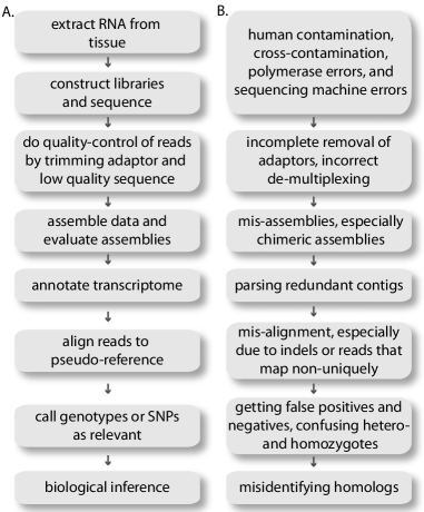
Figure 1: A. Pipeline for handling transcriptome data for de novo population genomic analyses, as presented in this study. B. Errors introduced at each stage in the pipeline.

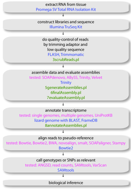
Figure 1: Pipeline used in this work, annotated to show (1) different approaches tested [pink], (2) the approach used for the final analysis [blue], and (3) scripts used, as named in the DataDryad package [green].

All bioinformatic pipelines are available as Perl scripts on https://sites.google.com/site/mvzseq/original-scripts-and-pipelines/pipelines, and they are summarized graphically in Figs. 1A and S1. I have also shared R scripts (R Development Core Team 2011) that use ggplot2 to do the statistical analyses and graphing presented in this paper (Wickham 2009).

2.1 Library Preparation and Sequencing

Even though costs of sequencing continue to drop and assembly methods improve (Glenn 2011; Schatz et al. 2010), whole-genome de novo sequencing remains inaccessible for researchers interested in organisms with large genomes (i.e., over 500 Mb) and for researchers who wish to sample variation at the population level. Thus, most de novo sequencing projects must still use some form of complexity reduction (i.e., target-based capture or restriction-based approaches) in order to interrogate a manageable portion of the genome. Here, I chose to sequence the transcriptome, because it is appropriately sized to ensure high coverage and successful de novo assembly, I will surely obtain homologous contigs across taxa, I can capture both functional and non-coding variation, and assembly can be validated by comparing to known protein-coding genes.

Liver and, where appropriate, testes samples were collected from adult male and female lizards during a field trip to Australia in fall 2010 (Table S1); tissues and specimens are accessioned at the Museum of Vertebrate Zoology, UC-Berkeley. I extracted total RNA from RNA-later preserved liver tissues using the Promega Total RNA SV Isolation kit. After checking RNA quality and quantity with a Bioanalyzer, I used the Illumina mRNA TruSeq kit to prepare individually barcoded cDNA libraries. Final libraries were quantified using qPCR, pooled at equimolar concentrations, and sequenced using four lanes of 100bp paired-end technology on the Illumina HiSeq2000.

2.2 Data Quality and Filtration

I evaluated raw data quality by using the FastQC module (Andrews 2012) and in-house Perl scripts that calculate sequencing error rate. Sequencing error rates for Illumina reads have been reported to be as high as 1% (Minoche et al. 2011); such high rates can both lead to poor assembly quality and false positive calls for SNPs. To compare to these reported values, I derived an empirical estimate of sequencing error rate. To do so, I aligned a random subsample of overlapping forward-reverse reads (N=100,000) using the local aligner blat (Kent 2002), identified mismatches and gaps, and calculated error rates as the total number of errors divided by double the length of aligned regions. Data were then cleaned: exact duplicates due to PCR amplification were removed, low-complexity reads (e.g., reads that consisted of homopolymer tracts or more than 20% ’N’s) were removed, reads were trimmed for adaptor sequence and for quality using a sliding window approach implemented in Trimmomatic (Lohse et al. 2012), reads matching contaminant sources (e.g., ribosomal RNA and human and bacterial sources) were removed via alignment to reference genomes with Bowtie2 (Langmead and Salzberg 2012), and overlapping paired reads were merged using Flash (Magoč and Salzberg 2011). Following data filtration but prior to read merging, I again estimated sequencing error rates using the method described above.

2.3 de novo Assembly

Determining what kmer, or nucmer length, to use is key in de novo assembly of genomic data (Earl et al. 2011). In assembling data with even coverage, researchers typically use just one kmer (Earl et al. 2011); however, with transcriptome data, contigs have uneven coverage because of gene expression differences (Martin and Wang 2011). Thus, some have shown the ideal strategy for transcriptomes is to assemble data at multiple kmers and then assemble across the assemblies to reduce redundancy (Surget-Groba and Montoya-Burgos 2010). To assemble across assemblies, I first identify similar contigs using clustering algorithms (cd-hit-est; (Li and Godzik 2006)) and local alignments (blat; (Kent 2002)) and then assemble similar contigs using a light-weight de novo assembler (cap3; (Huang and Madan 1999)). I used this multi-kmer, custom merge approach along with other existing approaches, including:

• A single kmer approach implemented in the program Trinity (a de novo RNA transcript assembler; (Grabherr et al. 2011))

• A single kmer approach implemented in ABySS (a de novo genomic assembler; (Simpson et al. 2009)), Velvet (a de novo genomic assembler; (Zerbino and Birney 2008)), and SOAPdenovo-Trans (a de novo RNA transcript assembler; (Li et al. 2010)), which I implemented as a multi-kmer approach using my custom merge script

• A multi-kmer approach implemented in the program OASES (Schulz et al. 2012)

I explore a wide-range of assembly methods because generating a high-quality and complete assembly is key for almost all downstream applications. Particularly with genome assembly, which is both an art and a science, researchers should try multiple approaches and evaluate their efficacy before further analyses (Earl et al. 2011). However, without a reference genome, evaluating the quality of a de novo assembly is challenging. Here, I implement novel metrics for evaluating de novo transcriptome assemblies. In addition to existing metrics in the literature (N50, mean contig length, total assembly length) (Martin and Wang 2011), I determined which proportion of reads were used in the assembly, measured putative levels of chimerism in transcripts due to misassemblies, determined the proportion of assembled transcripts that could be annotated and the accuracy of these transcripts (as determined by the number of nonsense mutations), and calculated the completeness and contiguity of the assembly (Martin and Wang 2011).

Here, I assembled across all individuals in a lineage rather than assembling each individual separately. Although this introduced additional polymorphism into the data which can reduce assembly efficiency (Vinson et al. 2005), previous work suggests the additional data lead to more complete assemblies (Singhal, unpublished).

2.4 Annotation

Following evaluation of my final assemblies, I chose the best assembly for annotation to protein databases. Determining the most appropriate database for annotation is important, so I tested multiple options, including using a single-species database, whether from a distantly-related but well-annotated genome or closely-related but poorly-annotated genome, using a multi-species database, or using a curated protein set, such as UniRef90 (Suzek et al. 2007). For one randomly selected lineage, I tested the efficiency and accuracy of five different reference databases:

• the non-redundant Ensembl protein database (Flicek et al. 2012) for the lizard Anolis carolinensis; with a most-recent common ancestor to my lineages of about $\approx$150 mya, it is the closest available genome (Alföldi et al. 2011),

• the non-redundant Ensembl protein data set for Gallus gallus, whose genome is higher quality than the Anolis genome but is more distantly related ($\approx$250 mya),

• a non-redundant, curated data set (UniRef90) of proteins from a wide range of organisms, whose genes have been clustered at 90% similarity,

• a highly-redundant Ensembl protein data set for eight vertebrates sequenced to high quality (human, dog, rat, mouse, platypus, opossum, dog, chicken),

• a highly-redundant Ensembl protein data set for the 54 vertebrates whose genomes have been annotated.

I evaluated the number of matching contigs, and for the non-redundant data sets, the number of uniquely matching contigs. Distinguishing between contigs that match and contigs that match uniquely is important, as despite my clustering during assembly, many contigs in the assembly appear redundant. These highly similar contigs likely result from misassemblies, allelic variants, alternative splicing isoforms, or recently duplicated paralogs. Parsing these categories is challenging without a reference genome and when expected coverage across contigs is uneven. Especially for projects interested in functional genomics, annotation of redundant contigs remains an important and unresolved issue. Here, I try to mitigate these errors by using reciprocal BLAST best matching to annotate contigs and selecting the best match. In doing so, I likely failed to annotate recently evolved paralogs, but I should not have multiple copies of the same gene in my downstream analyses.

Once I determined the best database both with respect to efficacy and efficiency, I used a custom script to annotate the contigs using a reciprocal best-match strategy via BLASTx and tBLASTx (Altschul et al. 1997) and defined the untranslated regions and coding sequence of the transcript using Exonerate (Slater and Birney 2005). Further, initial tests of the annotation pipeline uncovered two challenges: first, many contigs were chimeric and consisted of multiple, combined transcripts, and second, many of the predicted open reading frames (ORFs) had nonsense mutations, largely due to frameshift mutations. To address these problems, I identified chimeric contigs using BLASTx and split these contigs into individual genes, and I used the program FrameDP to identify and correct for frameshift mutations (Gouzy et al. 2009).

Finally, I searched unannotated contigs against the NCBI ’nr’ database using BLASTn to determine these contigs’ identity. As described in the Results, these unannotated contigs largely went unidentified. Thus, although some of these unannotated transcripts have viable open reading frames and/or had homologs in other lineages, and therefore, might be genes, I will be conservative and only use annotated transcripts in all downstream analyses.

Finally, to describe the putative biological functions of my annotated contigs, I determined gene ontology using Blast2Go (Conesa et al. 2005).

2.5 Alignment

The first step in identifying variants or estimating gene expression levels is to align the sequencing reads to one’s reference genome. Here, I use my annotated transcripts as a pseudo-reference genome (Wiedmann et al. 2008), thus aligning the reads used to generate the assembly to the assembly itself. Here, I tested six different aligners (bowtie, bowtie2, bwa, novoalign, smalt, SOAPaligner, stampy; Langmead et al. (2009); Langmead and Salzberg (2012); Li and Durbin (2009); Lunter and Goodson (2011); Li et al. (2008)) to determine their efficacy and accuracy. These programs run the gamut of being fast but less sensitive to being slower and more sensitive. Here, sensitivity is defined as the aligner’s ability to align reads with multiple mismatches. Previous results have shown (Li 2011) that alignment error is a common cause of miscalled SNPs, particularly alignment errors around indel sites. To evaluate these programs, I inferred genotypes from the alignments with SAMtools (Li et al. 2009). I then compared these genotypes to a small data set of known genotypes from one of the contact zones, C. rubrigularis N/S. In another study, I had Sanger sequenced 200-400 bp of sequence from 10 to 15 genes for the same individuals sequenced here (Singhal, unpublished). Importantly, all these genes were represented at high coverage ($\geq$20$\times$) in this data set; thus, coverage is sufficiently great to ensure accurate genotype calling. I used these validated genotypes to determine the number of false positives and negatives in my inferred genotypes. Further, I evaluated these programs based on the proportion of reads and read pairs they aligned and the concordance of SNP calls across data sets.

2.6 Variant discovery

Two major types of variant discovery are SNP identification and genotype calling. Many researchers are interested only in identifying SNPs, or determining which nucleotide positions are variable in a sample of individuals. SNP-containing regions are then resequenced or genotyped for further analysis (Wiedmann et al. 2008). Increasingly, researchers are both identifying variable sites, and then, summarizing variation at these sites using the site frequency spectrum (SFS) or calling genotype likelihoods for each individual for subsequent population genomics analyses. SNP identification has become an easier exercise as sequencing costs dropped and coverage has increased. However, genotype calling remains a challenging proposition, particularly in diploid and polyploid individuals, as distinguishing heterozygosity, homozygosity, and sequencing errors at variable sites is difficult unless there is high coverage ($\geq$20$\times$, Nielsen et al. (2012)). Thus, I focus on genotype calling and its use in characterizing variation for population genomics analyses. Importantly, I assume in my approach and discussion that both alleles are expressed in each individual; although there are some data to suggest that expression can be allele-biased (Palacios et al. 2009), accounting for this complexity is beyond the scope of this study.

My results indicated that Bowtie2 was the most effective and efficient aligner (see Results); thus, I used it for all downstream analyses. When identifying variants from alignment data, there are several approaches:

1. brute strength methods, in which the read counts for given alleles at a site are calculated, and variants are determined by an arbitrary cut-off (e.g. Yang et al 2011)

2. maximum likelihood (VarScan) and Bayesian methods (GATK, SAMtools) (Koboldt et al. 2009; DePristo et al. 2011; Li et al. 2009), in which algorithms consider strand bias, alignment quality, base quality, and depth to call genotype likelihoods for individuals. These methods have been developed further to account for Hardy-Weinberg disequilibrium and linkage disequilibrium in calling and filtering variants (Li et al. 2009; DePristo et al. 2011), to use machine learning with a set of validated SNPs to improve algorithms (DePristo et al. 2011), and to re-align reads near indel areas to ensure inaccurate alignments do not lead to false SNPs.

3. Bayesian methods (ANGSD) which infer the site frequency spectrum for all the variants in the data set, which in in turn, is used a prior to estimate genotype likelihoods for individuals (Nielsen et al. 2012). This method is particularly useful for data sets with large population samples.

Here, I test these three general types of SNP and genotype discovery, using read counting, VarScan, samtools, and ANGSD in two sister lineage-pairs for which I have validated genotypes (C. rubrigularis N/S and L. coggeri N/C). I both looked at concordance of SNP and genotype calls across methods and calculated the number of false positives and negatives.

2.7 Homolog discovery

Homologs between lineages must be identified for any comparative genomics analyses. In this study, my lineages are all closely-related, so homology identification is less challenging than in many other comparative studies. However, ensuring I am identifying orthologs across lineages and not paralogs is challenging, particularly as my annotation pipeline could not conclusively distinguish orthologs and paralogs in the absence of a reference genome. With that caveat, I test three different methods for identifying homology:

1. defining homologs by their annotation; i.e., contigs that share the same annotation are assumed to be homologs,

2. defining homologs by reciprocal best-hit BLAST, as is most commonly done in other studies (Moreno-Hagelsieb and Latimer 2008),

3. the SNP method, or defining homologs by mapping reads from one lineage to the other lineages’ assembly, identifying variants, and thus determining homologous sequence.

I evaluated these methods by the number of homologs found, the percent of aligned sequence between homologs, and the raw number of differences between homologous sequence. I looked at homology discovery both between sister lineages and non-sister lineages, as I expect discovery across non-sister lineages will be harder.

2.8 Biological inference

Finally, I determined how robust biological inference is to the analysis method used. First, to determine how genotype calling affects downstream inference, I inferred the site frequency spectrum and associated summary statistics (Tajima’s $D$, $\theta$, $\pi$) for one lineage across different genotype calling methods and different coverage levels. Second, to determine how homology identification affects downstream inference; I determined dN/dS ratios and raw sequence divergence for each gene across different methods of homology.

3 Results

3.1 Data Quality and Filtration

Library preparation and sequencing were successful for all individuals. On average, I generated 3.5 $\pm$ 0.5 Gb per individual. Duplication rates, low-complexity sequences, and contamination levels were low (Table S2). However, aggressive filtering and merging significantly reduced the raw data set; I lost 27.1 $\pm$ 3.8% of raw base pairs per individual. As seen in Figure S3, this strategy significantly improved the per-base quality of my data. Indeed, I was able to reduce sequencing error rates in my final data set five-fold (initial error rates: 0.3 $\pm$ 0.1%, final error rates: 0.06 $\pm$ 0.01%). These error rates are likely over-estimates, because I used the lower-quality portion of the read (the tail end) to identify sequencing errors. Despite this reduction in error rates, profiling of mismatches across the reads showed that both the head and tail of the read still harbor a higher number of mismatches compared to the rest of the read. This pattern persisted even when the first and last five base pairs of each read were trimmed prior to alignment (Fig. S4). Possibly, as others have found residual adaptor sequence in their data sets despite using rigorous adaptor trimming (Bi, unpublished; Almeida, unpublished), these heightened error rates could be due to adaptor sequences leading to misalignments and spurious SNPs.

3.2 de novo Assembly

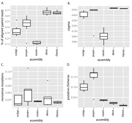
Figure 2: Evaluation of assemblies across the seven sequenced lineages according to A. percentage of paired reads that aligned to reference, B. number of CEGMA genes that are found in assembly, C. percentage of annotated coding sequences that had nonsense mutations, and D. percentage of contigs that were putative chimeras.

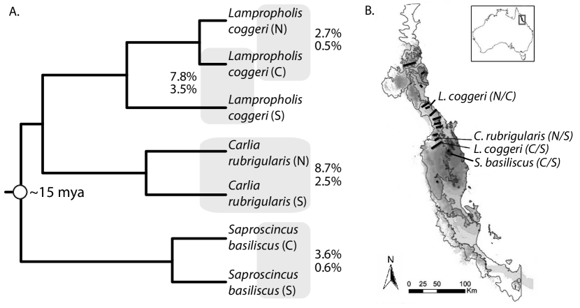
Figure 2: A. Phylogeny of the lineages studied in this work. Boxes indicate contacts studied; the top percentage reflects the mitochondrial divergence between lineages and the bottom is nuclear. B. A map of the Australian Wet Tropics, with all identified contact zones represented by black lines. Contacts of interest in this study are labelled.

To assemble my data, I tested five different programs, which employed different strategies (e.g., single k-mer, built-in multi-kmer approach, my custom multi-kmer approach). I evaluated the assemblies on many metrics; here, I show data for four of these metrics. With respect to the percentage of paired reads that aligned to the assembly, SOAPdenovo and Trinity performed far better than the rest of the assemblers (Fig. 2A), suggesting their assemblies were more contiguous. The same two assemblers and Velvet also recovered the greatest number of annotated transcripts, measured here by the number of core eukaryotic genes found in these assemblies (CEGMA; Parra et al. (2007); Fig. 2B). OASES and Trinity appeared to be the most accurate, as they contained the fewest number of nonsense mutations in annotated ORFs (Fig. 2C). Finally, OASES, Trinity and SOAPdenovo assemblies had the fewest number of putative chimeric transcripts (Fig. 2D). Looking across all these metrics, Trinity emerges as the best assembler. Further, Trinity did a good job assembling most of the data; on average, just 8.1 $\pm$ 4.3% of contigs from other assemblies were unique to that assembly compared to Trinity. As such, I used Trinity assemblies for all downstream analyses. As seen in Table 1, the basic metrics of these assemblies (e.g., number of contigs, total length of assembly, and N50) were fairly constant across all lineages. Unlike other studies (Comeault et al. 2012), I find no correlation between contig length and coverage, suggesting my assembly is not data-limited (Fig. S5).

3.3 Annotation

After assembling the data, I annotated the assemblies in order to identify unique, annotated contigs for downstream analyses and to refine the assemblies further. First, because my focal lineages are evolutionarily distant from the nearest genome (MRCA $\approx$150 mya to Anolis carolinensis), I wanted to test the efficacy of different databases to annotate my contigs. While more complete databases did lead more annotated contigs (Table S3), the increase was marginal. Further, larger databases consume significantly more computing time; here, annotating to the UniProt90 database took nearly 100 times the processor hours as annotating to A. carolinensis. Thus, I used the A. carolinensis database for all further annotations. Importantly, I could annotate these genomes to more distant relatives (G. gallus and T. guttata; MRCA $\approx$300 mya), without seeing a significant decrease in annotation success (Table S3). This result suggests such an annotation approach could work for organisms in even more genomically depauperate clades.

While annotating contigs, I identified a low percentage of chimeric contigs ($\approx$4%), which I resolved by splitting these contigs into individual genes (Table S4). Inspecting alignments of sequencing reads to these chimeric contigs suggested that these contigs form during assembly and not due to technical errors during library preparation, as chimeric junctions generally had significantly reduced coverage. Further, a small portion of the predicted open reading frames (ORFs) of annotated contigs ($\approx$3%) had premature stop codons. Although it is possible that these ORFs are pseudogenes (Kalyana-Sundaram et al. 2012), it seems more likely that they are due to assembly errors, as these contigs were generally highly expressed. Using FrameDP, I was able to identify and fix many of these likely frameshift errors (Table S4).

Through this pipeline, I annotated an average of 23360 contigs per lineage, of which, an average of 11366 contigs matched to a unique gene (Table 1). I also recovered the full coding sequence for many genes; 67% of unique annotated contigs encompassed the entire coding sequence for a gene, including portions of the 5’ and 3’ UTRs. These numbers appear reasonable – the annotation for the A. carolinensis genome currently includes 19K proteins, and liver tissue does not express all genes at a sufficiently high level to be represented here (Ramsköld et al. 2009). These genes contribute to a diversity of biological processes and serve a wide range of molecular functions, suggesting I assayed a varied portion of the transcriptome (Fig. S6).

Further, my pipeline appears to be robust; almost all unannotated contigs failed to find a good match in the NCBI ’nr’ database (Fig. S7). Approximately 9% of unannotated contigs matched to genes; however, further analysis of these matches showed that almost all of them matched with such low-quality to prevent annotation.

Additionally, by annotating contigs rigorously to limit the number of putative duplicate contigs, I significantly reduced the redundancy of my data set. When I aligned sequencing reads to my initial, unannotated assembly, I found that $\approx$10% of mapped reads aligned to multiple places in the assembly, suggesting a high level of redundancy. After annotating the genome and removing redundant contigs, I reduced the percentage of mapped reads aligning non-uniquely to $\approx$2%. However, removing redundant contigs also lead to an average 21% decline in reads mapped. Thus, it seems likely these redundant contigs are "biologically real", but we do not yet have the tools to parse such contigs properly (Vijay et al. in press).

3.4 Alignment

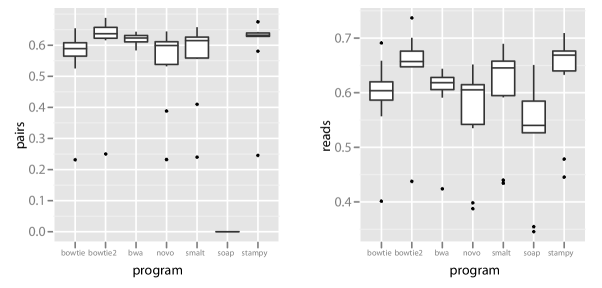
Figure 3: Evaluation of different alignment software across three randomly selected lineages with respect to two metrics, A. number of paired reads aligned and B. number of reads aligned.

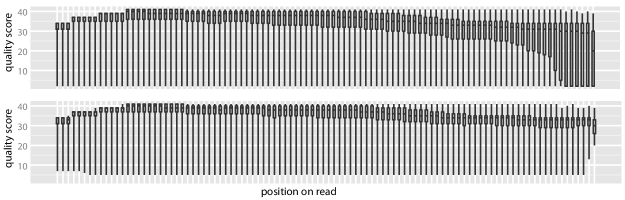
Figure 3: Quality scores in Phred along a read; top graph shows quality prior to cleaning and filtering, bottom shows quality after cleaning.

Identifying variants and quantifying gene expression first require that sequencing reads are aligned to the reference genome. Here, I tested the efficacy of seven different alignment programs, which employ different algorithms over a range of sensitivity and speed. I evaluated these programs in three ways. First, I used my externally validated set of genotypes to see how many genotypes were inferred correctly. Almost all of the aligners performed well and led to the correct genotype at $\geq$90% of the sites. Although the false negative rate was moderately high ($\approx$5% for most aligners), the false positive rate was low (Table 2). Bowtie2 clearly outperformed the rest of the aligners and was thus used for all downstream analyses. Second, I evaluated how many read pairs and reads the programs could align. Although Novoalign, smalt and stampy are generally considered to be more sensitive aligners, I found little variation in the percentage of reads aligned across programs (Fig. 3). Bowtie2 and stampy were able to align the most paired reads, which is useful as aligning paired reads reduces the likelihood of errant matches and non-unique matches (Bao et al. 2011). Finally, I looked at overlap in SNPs inferred across programs. Problematically, although all programs were fed the same reference genome and sequencing reads, I saw only moderate overlap – on average, only 77$\pm$9% of SNPs were shared. Checking the raw alignments suggested these discrepancies often arose from differences in alignment rather than differences in SNP inference post-alignment. These results suggest that alignment is likely a major source of error in de novo HTS analyses, as has been suggested by other studies (Li 2011; Lin et al. 2012; Kleinman and Majewski 2012). That said, when the same SNPs were called across programs, genotype inference was highly concordant; 94$\pm$2% of genotype calls were the same across alignment methods, and inferred allele frequency at these SNPs was highly correlated ($r$=0.94$\pm$0.01).

3.5 Variant Discovery

After alignment, programs for variant inference are used to call SNPs and genotypes. In the previous tests, I used the variant discovery program SAMtools for all analyses; here, I test a few approaches: a brute strength approach, in which I call SNPs and genotypes based solely on count data, two probabilistic methods (SAMtools and VarScan), and a probabilistic method that uses the allele frequency spectrum (ANGSD). I first assessed accuracy of genotype calls by using my externally validated genotype set. In general, I found that all methods performed fairly well – particularly, when a SNP was identified, all programs inferred the correct genotype with high accuracy ($\geq$98%; Table 3). However, the count method of identifying variation led to many false positives, an unsurprising result given its failure to account for sequence error or alignment score. ANGSD had a high false negative rate, the reason for which is unclear, though is possibly due to the small sample sizes used here. But, as shown by other work, ANGSD is best suited for correctly inferring the shape of the site frequency spectrum (Nielsen et al. 2012). Comparing across all SNPs found across all programs, I found that concordance across all SNPs was moderate, similar to my comparative alignment results. On average, only 83% of SNP calls are shared across programs. More promisingly, when a site is inferred as a SNP, 98% of the genotype calls are shared across programs. Overall, these results suggested SAMtools performed the best, so I used it for all downstream analyses.

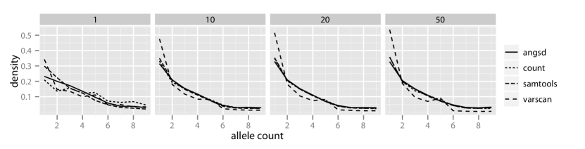
Figure 4: Unfolded allele frequency spectrum for variants within a randomly selected lineage for sites represented at 1x, 10x, 20x, and 50x coverage per individual, across different methods for genotype inference.

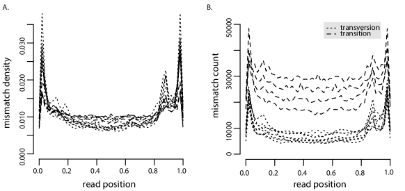
Figure 4: Identified mismatches between reads from a randomly-selected individual and the reference sequence, A. expressed in raw numbers and B. as a density distribution.

Upon defining SNPs and then genotypes for each individual, I explored how different variant discovery methods affect biological inference by constructing the SFS. Despite the only moderate levels of concordance in SNP calls, I find that the SFS is nearly identical across all the different approaches but VarScan (Fig. 4). Importantly, this result only holds true when I restrict analysis to higher-coverage contigs ($\geq$10$\times$); low-coverage contigs show aberrant patterns. Although the SFS is similar across all approaches, estimates of key population genetic summary statistics (i.e., $\theta_{w}$, $\pi$) vary depending on the approach – an unsurprising result given that the total number of SNPs inferred differs across approaches. Thus, prior to using these data for population genetic analyses, ascertainment bias must be factored into any downstream inference (citation). Finally, to look at these SNPs in greater detail, I annotated the SNPs I found in two sister-lineages, with respect to how they are segregating, their location relative to the gene, and their coding type (Fig. S9). Not only are the patterns of polymorphism and non-synonymous/synonymous mutations reasonable (Begun et al. 2011), but I also see that I have many types of variants (i.e., coding vs. non-coding, non-synonymous vs. synonymous, fixed vs. polymorphic), which will permit me to use the data to look for adaptive signatures of molecular evolution, infer demographic history, and to develop markers.

3.6 Homolog discovery

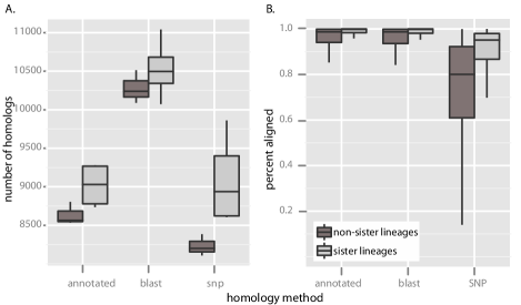
Figure 5: Summary of different methods for homolog discovery between all lineage comparisons of interest, considering A. number of homologs for which 75% of sequence was aligned and B. percent of homolog aligned.

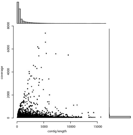
Figure 5: Correlation between contig length and coverage for a randomly-selected final assembly.

To identify homologs between lineages, I tested three different methods and then evaluated their effectiveness. All three methods performed well, identifying more than 8000 homologous pairs between lineages within-genera and between-genera for a significant portion of the contig length (Fig. 5). However, with the SNP method for homology, alignment efficiency dropped off significantly in between-genera comparisions, leading to identified homologs being shorter. I chose to use reciprocal BLAST matching to identify homologs for all downstream analyses as it was able to identify more homologs than the two other methods and it worked well across evolutionary distances (Fig. 5). This approach identified 8800 homologous contigs across all seven lineages for use in comparative analyses.

Estimation of the summary statistics (sequence divergence and $dN/dS$ ratios between homologs from lineage-pairs) is affected by how homologs are defined (Fig. S10). Defining homologs via annotation or via reciprocal BLAST matching gives very similar results for both sequence divergence and $dN/dS$. However, using SNPs to reconstruct the homolog results in a fuzzier pattern. This discrepancy likely stems from the many homologs for which coverage is low ($<$10$\times$), and thus, SNP inference is error-ridden (see Results: Variant Discovery). Thus, this method for homolog identification should account for differences in coverage, where appropriate.

4 Discussion

In creating and implementing a pipeline for high-throughput sequence data, I noted several possible sources of error (Fig. 1B):

1. Errors introduced during library preparation, which can include human contamination, errors introduced during PCR amplification of the library, and cross-contamination between samples

2. Errors introduced during sequencing, the frequency and type of which are dependent on the chemistry of sequencing platform, and subsequent de-multiplexing

3. Errors introduced during assembly (Baker 2012), such as misassembly of reads to create chimeric contigs

4. Errors due to misalignment of reads to assembly during variant discovery, particularly caused by indels in alignments and reads that map to multiple locations

5. Errors in SNP and genotype calling, such as not sampling both alleles and thus mistakenly calling a homozygote

To this, I add two additional sources of uncertainty that every study in evolutionary genomics faces – have contigs been annotated correctly and have orthologs between compared genomes been identified correctly (Chen et al. 2007)? Errors can arise at any stage in the process; such errors percolate through subsequent steps, likely affecting all downstream inference (Vijay et al. in press; Lin et al. 2012; Kleinman and Majewski 2012). Whether using their own pipeline or a pre-existing pipeline, researchers will want to incorporate some of the checks suggested here to ensure that the pipeline is working well for their data and that incidence of errors is low. Moving forward, the questions become how to limit these errors and how to mitigate their effects.

All these sources of error are non-trivial, but with careful data checking and willingness to discard low-quality data, I could mitigate the effects of these errors. I address these sources of error by stepping through the pipeline, explaining how I was able to reduce the error and identifying areas of future work. First, as has now become standard, scrubbing reads for low-quality bases and adaptors is a must – as shown here, read cleaning can reduce error rates noticeably. When possible, merging reads from paired-end reads can further decrease error rates and will lead to more accurate estimates of coverage for expression studies (Magoč and Salzberg 2011). Second, having a high-quality assembly is crucial both for accurate annotation and variant discovery. Inferring the quality of de novo assemblies is challenging, as there are no clear metrics or comparisons to use (Martin and Wang 2011). However, I propose a few metrics, which can be used with transcriptome data – primarily, looking for assemblies that minimize chimerism and non-sense mutations, that are contiguous, and that capture a significant portion of known key genes. Undoubtably, errors remain in the final assemblies, but these metrics helped me select the most accurate assembly for downstream analyses. Additionally, contig redundancy in final assemblies remains a pressing challenge. By using a strict reciprocal-BLAST annotation strategy, I removed many of these apparently redundant contigs. However, this approach certainly removed some biologically real contigs that were recent duplicates and alternative splicing isoforms fo interest to those interested in expression differences between biological groups (Vijay et al. in press). Researchers should continue to explore better methods to identify orthologs and paralogs.

Alignment and variant discovery remain notable challenges. In part, a poor-quality assembly genome truly can affect variant discovery – alignments across misassemblies can led to errant SNP calls, particularly when misassemblies introduce indels (Li 2011). Further, unless some sort of redundancy reduction is used, many contigs will be nearly identical in an assembly, leading to a high rate of non-unique alignments and miscalled SNPs. I was able to remove most redundant contigs, and thus, I reduced the proportion of non-unique alignments. I still see evidence for errors in alignment as (1) discrepancies between our externally-validated SNP set and genotype calls from these alignments and (2) the only moderate level of congruence between different approaches fueled by the same data. The same patterns hold for genotype inference based on alignment. My work here suggests, that given the data I have, the best approach is to rely on contigs with higher coverage – 10 to 20$\times$, at least – and to account for this ascertainment bias in any biological inference.

Further, to ensure the vagaries of variant discovery do not unduly influence our biological inference, we should use the genotype likelihoods and not genotype calls for downstream work. Ideally, researchers would conduct subsequent inference that use the SFS or genotype likelihoods as input, such as BAMOVA (Gompert and Buerkle 2011) or dadi (Gutenkunst et al. 2009), thus ensuring uncertainty in SNP and genotype calling is incorporated into model fitting. However, many analyses, particularly those used by most biodiversity researchers (i.e., coalescent-based demography and phylogeny programs), require known genotypes or haplotypes. Until uncertainty is incorporated into such programs, researchers will have to arbitrarily chose cutoffs to determine most likely genotypes. In such cases, researchers might want to restrict their analyses to regions with high coverage, where calls are likely more certain (Nielsen et al. 2012).

Moving forward, how can we reduce the sources of errors stemming from alignment errors and genotype inference? Improved assemblies, facilitated by new long-read sequencing technologies, will certainly help. As researchers collect externally validated SNP data sets, they can use programs like GATK to recalibrate variant calling and to realign around indels (DePristo et al. 2011). Researchers will also increasingly sequence more individuals in a population, which will better take advantage of multi-sample methods like samtools and ANGSD (Li et al. 2009; Nielsen et al. 2012). Finally, programs like Cortex, which assemble across individuals to provide both a reference assembly and individual assemblies, are promising. Simulations suggest that this method can also better handle data with indel polymorphism (Iqbal et al. 2012).

Finally, homolog discovery is a challenge in any genome project (Chen et al. 2007), and this project was no exception. All three methods I tested for homolog discovery worked well, but I recommend only using a SNP-based approach between lineages that are closely-related and for contigs with high coverage. Moving forward, as we acquire more comparative genomic data across the tree of life, homolog discovery should become an easier problem, as fueled by comparative clustering programs like OrthoMCL (Chen et al. 2005).

Through this work, I collated a large data set of over 12K annotated contigs, spanning a wide-range of biological functions, and over 100K SNPs between lineage-pairs, spanning a wide-range of locations and coding types. Notably, I was able to do all of these analyses using existing, open-source software and, but for assembly, by using a low-end desktop machine. Genomic analyses are not just for those working with humans or mice anymore. With careful and thoughtful data curation, HTS can enable researchers to use genomic approaches to explore all the branches in the tree of life.

5 Acknowledgements

I gratefully acknowledge M. Chung, J. Penalba, and L. Smith for technical support, and the Seqanswers.com community for providing timely and thoughtful advice. R. Bell, K. Bi, J. Bragg, T. Linderoth, M. MacManes, C. Moritz, R. Nielsen, S. Ramirez, F. Zapata, and members of the Moritz Lab Group provided comments and suggestions during this work and on this manuscript that greatly improved its quality. Financial support for this work was provided by National Science Foundation (Graduate Research Fellowship and Doctoral Dissertation Improvement Grant), the Museum of Vertebrate Zoology Wolff Fund, and a Rosemary Grant Award from the Society of the Study of Evolution. This work was made possible by the supercomputing resources provided by NSF XSEDE, in particular the clusters at Texas Advanced Computing Center and Pittsburgh Supercomputing Center.

6 Tables

assembly	number contigs	total length	n50	annotated contigs	annotated contigs (unique)	complete annotated contigs
C. rubrigularis, N	104648	89.1e6	1806	25198	12063	8179
C. rubrigularis, S	98280	84.3e6	1780	24323	11558	7697
L. coggeri, N	96798	87.5e6	1972	22760	11457	7344
L. coggeri, C	106937	92.7e6	1845	23852	10894	7796
L. coggeri, S	112935	89.6e6	1549	23774	11029	7258
S. basiliscus, C	84756	77.7e6	1951	21584	11221	7586
S. basiliscus, S	98685	83.5e6	1749	22031	11340	7696

Table 1: Summary of assemblies and their annotation. Complete annotated contigs are those with some 5’ and 3’ UTR sequence, as well as the full coding sequence.

genotype	bowtie	bowtie2	bwa	novoalign	smalt	SOAPaligner	stampy
right genotype	379 (89.8%)	419 (99.2%)	381 (90.3%)	383 (90.8%)	393 (93.1%)	207 (49.0%)	391 (92.7%)
wrong genotype	29 (6.9%)	3 (0.7%)	7 (1.7%)	9 (2.1%)	6 (1.4%)	52 (12.3%)	8 (1.9%)
false negative	12 (2.8%)	0 (0%)	34 (8.1%)	30 (7.1%)	23 (5.5%)	163 (38.6%)	23 (5.5%)
false positive	3	1	1	1	1	1	5

Table 2: Accuracy of genotype inference following the use of different programs for alignment; all genotypes were inferred using samtools post-alignment. Parenthetical percentages show the relative proportions of genotype types.

Genotype	ANGSD	count data	SAMtools	VarScan
right genotype	520 (68.4%)	745 (98.0%)	750 (98.7%)	745 (98.0%)
wrong genotype	3 (0.3%)	15 (2.0%)	10 (1.3%)	15 (2.0%)
false negative	230 (30.2%)	0 (0%)	0 (0%)	0 (0%)
false positive	6	134	1	12

Table 3: Accuracy of genotype inference across different programs for genotype inference; for all, Bowtie2 was used for alignment. Parenthetical percentages show the relative proportions of genotype types.

7 Figures

8 Supplementary Tables

individual	lineage	latitude	longitude	Locality
SS34	C. rubrigularis N	-16.617	145.458	Mount Harris
SS35	C. rubrigularis N	-16.617	145.458	Mount Harris
SS37	C. rubrigularis N	-16.611	145.452	Mount Harris
SS40	C. rubrigularis N	-16.611	145.452	Mount Harris
SS41	C. rubrigularis N	-16.611	145.452	Mount Harris
SS48	C. rubrigularis S	-17.694	145.694	S. Johnstone River, Sutties Gap Rd
SS50	C. rubrigularis S	-17.694	145.694	S. Johnstone River, Sutties Gap Rd
SS52	C. rubrigularis S	-17.660	145.722	S. Johnstone River, Sutties Gap Rd
SS56	C. rubrigularis S	-17.678	145.710	S. Johnstone River, Sutties Gap Rd
SS57	C. rubrigularis S	-17.678	145.710	S. Johnstone River, Sutties Gap Rd
SEW08448	L. coggeri C	-16.976	145.777	Lake Morris Rd
SEW08452	L. coggeri C	-16.976	145.777	Lake Morris Rd
SS135	L. coggeri C	-16.976	145.777	Lake Morris Rd
SS136	L. coggeri C	-16.976	145.777	Lake Morris Rd
SS138	L. coggeri C	-16.976	145.777	Lake Morris Rd
SS64	L. coggeri N	-16.579	145.315	Mount Lewis
SS65	L. coggeri N	-16.572	145.322	Mount Lewis
SS67	L. coggeri N	-16.578	145.308	Mount Lewis
SS72	L. coggeri N	-16.585	145.289	Mount Lewis
SS74	L. coggeri N	-16.584	145.302	Mount Lewis
SS54	L. coggeri S	-17.660	145.722	S. Johnstone River, Sutties Gap Rd
SS59	L. coggeri S	-17.700	145.693	S. Johnstone River, Sutties Gap Rd
SS60	L. coggeri S	-17.700	145.693	S. Johnstone River, Sutties Gap Rd
SS62	L. coggeri S	-17.676	145.713	S. Johnstone River, Sutties Gap Rd
SS63	L. coggeri S	-17.628	145.740	S. Johnstone River, Sutties Gap Rd
SS25	S. basiliscus C	-17.295	145.712	Butchers Creek
SS28	S. basiliscus C	-17.299	145.701	Butchers Creek
SS29	S. basiliscus C	-17.299	145.701	Butchers Creek
SS30	S. basiliscus C	-17.299	145.701	Butchers Creek
SS32	S. basiliscus C	-17.299	145.701	Butchers Creek
SS127	S. basiliscus S	-18.199	145.849	Kirrama Range Rd
SS128	S. basiliscus S	-18.199	145.849	Kirrama Range Rd
SS129	S. basiliscus S	-18.199	145.849	Kirrama Range Rd
SS130	S. basiliscus S	-18.199	145.849	Kirrama Range Rd
SS131	S. basiliscus S	-18.199	145.849	Kirrama Range Rd

Table 1: Individuals included in this study and their associated locality data.

filtering type	rate
duplication	1.4 $\pm$ 0.2%
contamination	0.4 $\pm$ 1.1%
low-complexity reads	0.004 $\pm$ 0.003%
merging reads	68.7 $\pm$ 4.7%

Table 2: Quality control filtering and their rates in raw data, summarized across seven lineages.

database	annotated contigs	unique, annotated contigs
A. carolinensis	23804	12218
G. gallus	22324	11146
UniProt90 database	26089	12324
Ensembl 9-species database	25838	NA
Ensembl 54-species database	26601	NA

Table 3: Number of contigs annotated according to different reference databases for a randomly selected assembly.

assembly	initial chimerism	final chimerism	initial stop codons	final stop codons
C. rubrigularis, N	4.6%	0.0%	2.6%	0.6%
C. rubrigularis, S	3.7%	0.0%	2.8%	0.8%
L. coggeri, N	10.3%	0.0%	3.3%	1.1%
L. coggeri, C	5.5%	0.0%	3.1%	1.0%
L. coggeri, S	3.9%	0.0%	3.3%	1.0%
S. basiliscus, C	4.4%	0.0%	2.6%	0.6%
S. basiliscus, S	4.0%	0.0%	2.8%	0.7%

Table 4: Prevalence of chimerism, or percentage of contigs that appeared to consist of multiple genes misassembled together, and stop codons, or percentage of contigs that had nonsense mutations, in assemblies, summarized across seven lineages both before and after the data were run in the annotation pipeline.

coverage	number of contigs within lineage	number of contigs between lineages
10x	3326 $\pm$ 494	2606 $\pm$ 399
20x	1888 $\pm$ 316	1439 $\pm$ 245
30x	1311 $\pm$ 245	981 $\pm$ 178
40x	994 $\pm$ 190	741 $\pm$ 133
50x	808 $\pm$ 157	602 $\pm$ 108

Table 5: Number of annotated contigs which have given coverage for each individual; shown for one randomly selected lineage-pair.

9 Supplementary Figures

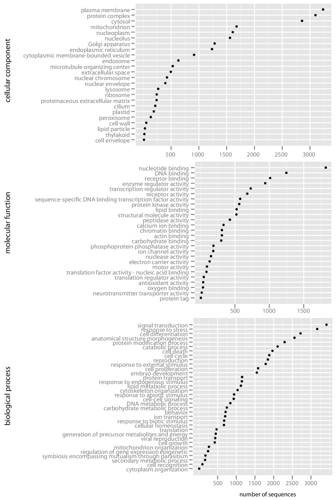
Figure 6: Gene ontology for annotated contigs for a randomly-selected lineage, with respect to cellular component, biological process, and molecular function.

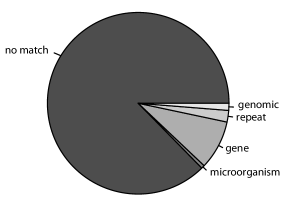
Figure 7: Identify of unannotated contigs from a randomly selected assembly, as identified from a BLAST search to the NCBI ’nr’ nucleotide database.

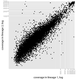
Figure 8: Correlation in coverage between homologous, annotated contigs for a randomly-selected lineage-pair.

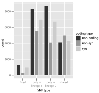
Figure 9: Summary of SNPs found in a randomly-selected lineage-pair, annotated with respect to SNP and coding type.

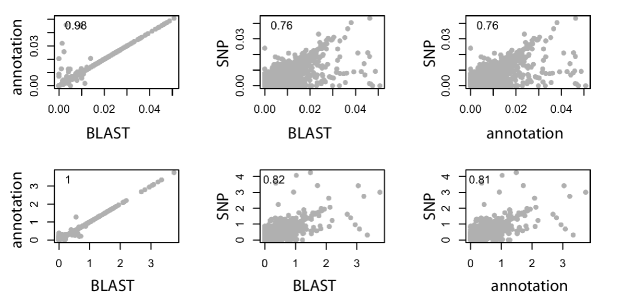
Figure 10: Top row shows correlation in sequence divergence and bottom row shows correlation in inferred $dN/dS$ ratios for homologs for a randomly-selected lineage-pair for three methods of homolog discovery.

References

- Alföldi et al. (2011) Alföldi, J., F. D. Palma, M. Grabherr, C. Williams, L. Kong, E. Mauceli, P. Russell, C. Lowe, R. Glor, J. Jaffe, D. Ray, S. Boissinot, A. Shedlock, C. Botka, T. Castoe, J. Colbourne, M. Fujita, R. Moreno, B. ten Hallers, D. Haussler, A. Heger, D. Helman, D. Janes, J. Johnson, P. de Jong, M. Koriabine, M. Lara, P. Novick, C. Organ, S. Peach, S. Poe, D. Pollock, K. de Queiroz, T. Sanger, S. Searle, J. Smith, Z. Smith, R. Swofford, J. Turner-Maier, J. Wade, S. Young, A. Zadissa, S. Edwards, T. Glenn, C. Schneider, J. Losos, E. Lander, M. Breen, C. Ponting, and K. Lindblad-Toh, 2011. The genome of the green anole lizard and a comparative analysis with birds and mammals. Nature 477:587–591.
- Altschul et al. (1997) Altschul, S., T. Madden, A. Schaffer, J. Zhang, Z. Zhang, W. Miller, and D. Lipman, 1997. Gapped BLAST and PSI-BLAST: a new generation of protein database search programs. Nucleic Acids Research 25:3389–3402.
- Andrews (2012) Andrews, S., 2012. FastQC. URL http://www.bioinformatics.babraham.ac.uk/projects/fastqc/.
- Baker (2012) Baker, M., 2012. de novo genome assembly: what every biologist should know. Nature Methods 9:333–337.
- Bao et al. (2011) Bao, S., R. Jiang, W. Kwan, B. Wang, X. Ma, and Y. Song, 2011. Evaluation of next-generation sequencing software in mapping and assembly. Journal of Human Genetics 56:406–414.
- Begun et al. (2011) Begun, D., A. Holloway, K. Stevens, L. Hillier, Y. Poh, M. Hahn, P. Nista, C. Jones, A. Kern, C. Dewey, L. Pachter, E. Myers, and C. Langley, 2011. Population genomics: whole-genome analysis of polymorphism and divergence in Drosophila simulans. PLoS Biology 5:310.
- Catchen et al. (2011) Catchen, J., A. Amores, P. Hohenlohe, W. Cresko, and J. Postlethwait, 2011. Stacks: building and genotyping loci de novo from short read sequences. Genes, Genomes, Genetics 1:171–182.
- Chen et al. (2005) Chen, F., A. Mackey, C. S. Jr., and D. Roos, 2005. OrthoMCL-DB: querying a comprehensive multi-species collection of ortholog groups. Nucleic Acids Research 34:363–368.
- Chen et al. (2007) Chen, F., A. Mackey, J. Vermunt, and D. Roos, 2007. Assessing performance of orthology detection strategies applied to eukaryotic genomes. PLoS ONE 2:383.
- Comeault et al. (2012) Comeault, A., M. Sommers, T. Schwander, C. Buerkle, T. Farkas, P. Nosil, and T. Parchman, 2012. De novo characterization of the Timema cristinae transcriptome facilitates marker discovery and inference of genetic divergence. Molecular Ecology Resources 12:549–61.
- Conesa et al. (2005) Conesa, A., S. Gotz, J. Garcia-Gomez, J. Terol, M. Talon, and M. Robles, 2005. Blast2GO: a universal tool for annotation, visualization and analysis in functional genomics research. Bioinformatics 15:3674–6.
- de Wit et al. (2012) de Wit, P., M. Pespeni, J. Ladner, D. Barshis, F. Seneca, H. Jaris, N. Therkildsen, M. Morikawa, and S. Palumbi, 2012. The simple fool’s guide to population genomics via RNA-seq: an introduction to high-throughput sequencing data analysis. Molecular Ecology Resources 12:1058–1067.
- DePristo et al. (2011) DePristo, M., E. Banks, R. Poplin, K. Garimella, J. Maguire, C. Hartl, A. Philippakis, G. del Angel, M. Rivas, M. Hanna, A. McKenna, T. Fennell, A. Kernytsky, A. Sivachenko, K. Cibulskis, S. G. dn D. Altschuler, and M. Daly, 2011. A framework for variation discovery and genotyping using next-generation DNA sequencing data. Nature Genetics 43:491–8.
- Earl et al. (2011) Earl, D., K. Bradnam, J. S. John, A. Darlin, D. Lin, J. Fass, H. Yu, V. Buffalo, D. Zerbino, M. Diekhans, N. Nguyen, P. Ariyaratne, W. Sung, Z. Ning, M. Haimel, J. Simpson, N. Fonseca, I. Birol, T. Docking, I. Ho, D. Rokhsar, R. CHikhi, D. Lavenier, G. Chapuis, D. Naquin, N. Maillet, M. Schatz, D. Kelley, A. Phillippy, S. Koren, S. Yang, W. Wu, W. Chou, A. Srivastava, T. Shaw, J. Ruby, P. Skewes-Cox, M. Betegon, M. Dimon, V. Solovyev, I. Seledtscov, P. Kosarev, D. Vorobyev, R. Ramirez-Gonzalez, R. Leggett, D. MaclEan, F. Xia, R. Luo, Z. Li, Y. Xie, B. Liu, S. Gnerre, I. MacCallum, D. Przybylski, F. Ribeiro, S. Yin, T. Sharpe, G. Hall, P. Kersey, R. Durbin, S. Jackman, J. Chapman, X. Huang, J. DeRisi, M. Caccamo, Y. Li, D. Jaffe, R. Green, D. Haussler, I. Korf, and B. Paten, 2011. Assemblathon 1: a competitive assessment of de novo short read assembly methods. Genome Research 21:2224–41.
- Ellegren et al. (2012) Ellegren, H., L. S. an dR. Burri, P. Olason, N. Backstrom, T. Kawakami, A. Kunstner, H. Makinen, K. Nadachowska-Bryzska, A. Q. adn S. Uebbing, and J. Wolf, 2012. The genomic landscape of species divergence in Ficedula flycatchers. Nature in press.
- Flicek et al. (2012) Flicek, P., M. Amode, D. Barrell, K. Beal, S. Brent, D. Carvalho-Silva, P. Clapham, G. Coates, S. Fairley, S. Fitzgerald, L. Gil, L. Gordon, M. Hendrix, T. Hourlier, N. Johnson, A. Kahari, D. Keefe, S. Keenan, R. Kinsella, M. Komorowska, G. Koscielny, E. Kulesha, P. Larsson, I. Longden, W. McLaren, M. Muffato, B. Overduin, M. Pignatelli, B. Pritchard, H. Riat, G. Ritchie, M. Ruffier, M. Schuster, D. Sobral, Y. Tang, K. Taylor, S. Trevanion, J. Vandrovcova, S. White, M. Wilson, S. Wilder, B. Aken, E. Birney, F. Cunningham, I. Dunham, R. Durbin, X. Fernandez-Suarez, J. Harrow, J. Herrero, T. Hubbard, A. Parker, G. Proctor, G. Spudich, J. Vogel, A. Yates, A. Zadissa, and S. Searle, 2012. Ensembl 2012. Nucleic Acids Research 40:84–90.
- Glenn (2011) Glenn, T., 2011. Field guide to next-generation DNA sequencers. Molecular Ecology Resources 11:759–769.
- Gompert and Buerkle (2011) Gompert, Z. and C. Buerkle, 2011. A hierarchical Bayesian model for next-generation population genomics. Genetics 187:903–917.
- Gouzy et al. (2009) Gouzy, J., S. Careere, and T. Schiex, 2009. FrameDP: sensitive peptide detection on noisy matured sequences. Bioinformatics 25:670–671.
- Grabherr et al. (2011) Grabherr, M., B. Haas, M. Yassour, J. Levin, D. Thompson, I. Amit, x. Adiconis, L. Fan, R. Raychowdury, Q. Zeng, Z. Chen, E. Mauceli, N. Hacohen, A. Gnike, N. Rhind, F. di Palma, B. Birren, C. Nusbaum, K. Lindblad-Toh, N. Friedman, and A. Regev, 2011. Full-length transcriptome assembly from RNA-Seq data without a reference genome. Nature Biotechnology 15:644–652.
- Gutenkunst et al. (2009) Gutenkunst, R., R. Hernandez, S. Williamson, and C. Bustamante, 2009. Inferring the joint demographic history of multiple populations from multidimensional SNP frequency data. PLoS Genetics 5:1000695.
- Hird et al. (2011) Hird, S., R. Brumfield, and B. Carstens, 2011. PRGmatic: an efficient pipeline for collating genome-enriched second-generation sequencing data using a ’provisional reference genome’. Molecular Ecology Resources 11:743–748.
- Hohenlohe et al. (2010) Hohenlohe, P., S. Bassham, P. Etter, N. Stiffler, E. Johnson, and W. Cresko, 2010. Population genomics of parallel adaptation in threespine stickleback using sequenced RAD tags. PLoS Genetics 6:1000862.
- Huang and Madan (1999) Huang, X. and A. Madan, 1999. CAP3: a DNA sequence assembly program. Genome Research 9:868–77.
- Iqbal et al. (2012) Iqbal, Z., M. Caccamo, I. Turner, P. Flicek, and G. McVean, 2012. De novo assembly and genotyping of variants using colored de Bruijn graphs. Nature Genetics 44:226–232.
- Kalyana-Sundaram et al. (2012) Kalyana-Sundaram, S., C. Kumar-Sinha, S. Shankar, D. Robinson, Y. Wu, X. Cao, I. Asangani, V. Kothari, J. Prensner, R. Lonigro, M. Iyer, T. Barrette, A. Chanmugam, S. Dhanasekaran, N. Panisamy, and A. Chinnaiyan, 2012. Expressed pseudogenes in the transcriptional landscape of human cancers. Cell 149:1622–1634.
- Keller et al. (2012) Keller, I., C. Wagner, L. Greuter, S. Mwaiko, O. Selz, A. Sivasundar, S. Wittwer, and O. Seehausen, 2012. Population genomic signatures of divergent adaptation, geneflow and hybrid speciation in the rapid radiation of Lake Victoria cichlid fishes. Molecular Ecology in press.
- Kent (2002) Kent, W., 2002. BLAT–the BLAST-like alignment tool. Genome Research 12:656–64.
- Kleinman and Majewski (2012) Kleinman, C. and J. Majewski, 2012. Comment on "Widespread RNA and DNA sequence differences in the human transcriptome". Science 335:1302.
- Koboldt et al. (2009) Koboldt, D., K. Chena, T. Wylie, D. Larsona, M. McLellan, E. Mardis, G. Weinstock, R. Wilson, and L. Ding, 2009. VarScan: variant detection in massively parallel sequencing of individual and pooled samples. Bioinformatics 25:2283–5.
- Langmead and Salzberg (2012) Langmead, B. and S. Salzberg, 2012. Fast gapped-read alignment with Bowtie 2. Nature Methods 9:357–359.
- Langmead et al. (2009) Langmead, B., C. Trapnell, M. Pop, and S. Salzberg, 2009. Ultrafast and memory-efficient alignment of short DNA sequences to the human genome. Genome Biology 10:25.
- Li (2011) Li, H., 2011. A statistical framework for SNP calling, mutation discovery,association mapping and population genetical parameter estimation from sequencing data. Bioinformatics 27:2987–2993.
- Li and Durbin (2009) Li, H. and R. Durbin, 2009. Fast and accurate short read alignment with Burrows-Wheeler transform. Bioinformatics 25:1754–1760.
- Li et al. (2009) Li, H., B. Handsaker, A. Wysoker, T. Fennell, J. Ruan, N. Homer, G. Marth, G. Abecasis, R. Durbin, and 1000 Genome Project Data Processing Subgroup, 2009. The sequence alignment/map (SAM) format and SAMtools. Bioinformatics 25:2078–2079.
- Li et al. (2008) Li, R., Y. Li, K. Kristiansen, and J. Wang, 2008. SOAP: short oligonucleotide alignment program. Bioinformatics 24:713–714.
- Li et al. (2010) Li, R., H. Zhu, J. Ruan, W. Qian, X. Fang, Z. Shi, Y. Li, S. Li, G. Shan, K. Kristiansen, S. Li, H. Yang, J. Wang, and J. Wang, 2010. De novo assembly of human genomes with massively parallel short read sequencing. Genome Research 20:265–272.
- Li and Godzik (2006) Li, W. and A. Godzik, 2006. CD-Hit: a fast program for clustering and coomparing large sets of protein or nucleotide sequences. Bioinformatics 22:1658–59.
- Lin et al. (2012) Lin, W., R. Piskol, M. Tan, and J. Li, 2012. Comment on "Widespread RNA and DNA sequence differences in the human transcriptome". Science 335:1302.
- Lohse et al. (2012) Lohse, M., A. Bolger, A. Nagel, A. Fernie, J. Lunn, M. Stitt, and B. Usadel, 2012. RobiNA: a user-friendly, integrated software solution for RNA-Seq-based transcriptomics. Nucleic Acids Research 40:622–7.
- Luca et al. (2011) Luca, F., R. Hudson, D. Witonsky, and A. D. Rienzo, 2011. A reduced representation approach to population genetic analyses and applications to human evolution. Genome Research 21:1087–1098.
- Lunter and Goodson (2011) Lunter, G. and M. Goodson, 2011. Stampy: A statistical algorithm for sensitive and fast mapping of Illumina sequence reads. Genome Research 21:936–939.
- Magoč and Salzberg (2011) Magoč, T. and S. Salzberg, 2011. FLASH: fast length adjustment of short reads to improve genome assemblies. Bioinformatics 27:2957–63.
- Martin and Wang (2011) Martin, J. and Z. Wang, 2011. Next-generation transcriptome assembly. Nature Reviews Genetics 12:671–682.
- Minoche et al. (2011) Minoche, A., J. Dohm, and H. Himmelbauer, 2011. Evaluation of genomic high-throughput sequencing data generated on Illumina HiSeq and Genome Analyzer systems. Genome Biology 12:112.
- Moreno-Hagelsieb and Latimer (2008) Moreno-Hagelsieb, G. and K. Latimer, 2008. Choosing BLAST options for better detection of orthologs as reciprocal best hits. Bioinformatics 24:319–324.
- Nielsen et al. (2012) Nielsen, R., T. Korneliussen, A. Albrechtsen, Y. Li, and J. Wang, 2012. SNP calling, genotype calling, and sample allele frequency estimation from new-generation sequencing data. PLoS One 7:37558.
- Nielsen et al. (2011) Nielsen, R., J. Paul, A. Albrechtsen, and Y. Song, 2011. Genotype and SNP calling from next-generation sequencing data. Nature Review Genetics 12:443–51.
- Palacios et al. (2009) Palacios, R., E. Gazave, J. Goni, G. Piedafita, O. Fernando, A. Navarro, and P. Villoslada, 2009. Allele-specific gene expression is widespread across the genome and biological process. PLoS One 4:4150.
- Parra et al. (2007) Parra, G., K. Bradnam, and I. Korf, 2007. CEGMA: a pipeline to accurately annotate core genes in eukaryotic genomes. Bioinformatics 23:1061–67.
- R Development Core Team (2011) R Development Core Team, 2011. R: A Language and Environment for Statistical Computing. R Foundation for Statistical Computing, Vienna, Austria. URL http://www.R-project.org. ISBN 3-900051-07-0.
- Ramsköld et al. (2009) Ramsköld, D., E. Wang, C. Burge, and R. Sandberg, 2009. An abundance of ubiquitously expressed genes revealed by tissue transcriptome sequence data. PLoS Computational Biology 5:1000598.
- Schatz et al. (2010) Schatz, M., A. Delcher, and S. Salzberg, 2010. Assembly of large genomes using second-generation sequencing. Genome Research 20:1165–73.
- Schulz et al. (2012) Schulz, M., D. Zerbino, M. Vingron, and E. Birney, 2012. Oases: robust de novo RNA-seq assembly across the dynamic range of expression levels. Bioinformatics 28:1086–1092.
- Simpson et al. (2009) Simpson, J., K. Wong, S. Jackman, J. Schein, S. Jones, and I. Birol, 2009. ABySS: a parallel assembler for short read sequence data. Genome Research 19:1117–1123.
- Singhal and Moritz (2012) Singhal, S. and C. Moritz, 2012. Strong selection against hybrids maintains a narrow contact zone between morphologically cryptic lineages in a rainforest lizard. Evolution 66:1474–89.
- Skinner et al. (2011) Skinner, A., A. Hugall, and A. Hutchinson, 2011. Lygosomine phylogeny and the origins of Australian scincid lizards. Journal of Biogeography 38:1044–1058.
- Slater and Birney (2005) Slater, G. and E. Birney, 2005. Automated generation of heuristics for biological sequence comparison. BMC Bioinformatics 6:31.
- Smith et al. (2011) Smith, S., N. Wilson, F. Goetz, C. Feehery, S. Andrade, G. Rouse, G. Giribet, and C. Dunn, 2011. Resolving the evolutionary relationships of molluscs with phylogenomic tools. Nature 480:364–367.
- Surget-Groba and Montoya-Burgos (2010) Surget-Groba, Y. and J. Montoya-Burgos, 2010. Optimization of de novo transcriptome assembly from next-generation sequencing data. Genome Research 20:1432–40.
- Suzek et al. (2007) Suzek, B., H. Huang, P. McGarvey, R. Mazumder, and C. Wu, 2007. UniRef: comprehensive and non-redundant UniProt reference clusters. Bioinformatics 23:1282–8.
- Vijay et al. (in press) Vijay, N., J. Poelstra, A. Kunstner, and J. Wolf, in press. Challenges and strategies in transcriptome assembly and differential gene expression quantification. a comprehensive in silico assessment of RNA-seq experiments. Molecular Ecology .
- Vinson et al. (2005) Vinson, J., D. Jaffe, K. O’Neill, E. Karlsson, N. S.-T. an S. Anderson, J. Mesirove, N. Satoh, Y. Satou, C. Nusbaum, B. Birren, J. Galagan, and E. Lander, 2005. Assembly of polymorphic genomes: Algorithms and application to Ciona savignyi. Genome Research 15:1127–1135.
- Wickham (2009) Wickham, H., 2009. ggplot2: elegant graphics for data analysis. Springer New York. URL http://had.co.nz/ggplot2/book.
- Wiedmann et al. (2008) Wiedmann, R., T. Smith, and D. Nonneman, 2008. SNP discovery in swine by reduced representation and high throughput pyrosequencing. BMC Genetics 9:81.
- Yi et al. (2010) Yi, X., Y. Liang, E. Huerta-Sanchez, . Jin, Z. Cuo, J. P. an X. Xu, H. Jiang, N. Vinckenbosch, T. Korneliussen, H. Zheng, T. Liu, W. He, K. Li, R. Luo, X. Nie, H. Wu, M. Zhao, H. Cao, J. Zou, Y. Shan, S. Li, Q. Yang, Asan, P. Ni, G. Tian, J. Xu, X. Liu, T. jiang, R. Wu, G. Zhou, M. Tang, J. Qin, T. Wang, S. Feng, G. Li, Huasang, J. Luosang, W. Wang, F. Chen, Y. Wang, X. Zheng, Z. Li, Z. Bianba, G. Yang, X. Wang, S. Tang, G. Gao, Y. Chen, Z. Luo, L. Gusang, Z. Cao, Q. Zhang, W. Ouyang, X. Ren, H. Liang, H. Zheng, Y. Huang, J. Li, L. Bolund, K. Kristiansen, Y. Li, Y. Zhang, X. Zhang, R. Li, S. Li, H. Yang, R. Nielsen, J. Wang, and J. Wang, 2010. Sequencing of 50 human exomes reveals adaptation to high altitude. Science 329:75–78.
- Zerbino and Birney (2008) Zerbino, D. and E. Birney, 2008. Velvet: algorithms for de novo short read assembly using de Bruijn graphs. Genome Research 18:821–829.