An estimate of heavy quark momentum diffusion coefficient in gluon plasma

Abstract:

We calculate the momentum diffusion coefficient for heavy quarks in SU(3) gluon plasma at temperatures 1-2 times the deconfinement temperature. The momentum diffusion coefficient is extracted from a Monte Carlo calculation of the correlation function of color electric fields, in the leading order of expansion in heavy quark mass. Systematics of the calculation are examined, and compared with perturbtion theory and other estimates.

1 Introduction

The charm and bottom quarks play a very important role as probes of the medium created in relativistic heavy ion collision experiments. Since the masses of both these quarks are considerably larger than the temperatures estimated to have been reached in RHIC and even in LHC, one expects these quarks to be produced largely in the early state of the collision. They therefore allow us to look at the medium at its early times. Besides, since the nature of energy loss and of collective behavior of the heavy quarks are different from those of the light quarks, a study of the heavy quark jets and the flow of the heavy hadrons leads to crucial insights into the way the medium interacts.

As collision with a thermal quark does not change the energy of a heavy quark substantially, one would expect the thermalization time of the heavy quark to be large. Since elliptic flow develops early, it is reasonable to expect that the elliptic flow will show a mass hierarchy: $v_{2}^{h}\gg v_{2}^{D}\gg v_{2}^{B}$, where D and B refer to generic mesons in D (one valence charm) and B (one valence bottom) family, and $h$ refers to the light hadrons. Similarly, the nuclear suppression factor can be intuitively expected to be closer to 1 for the heavy-light mesons: $R^{h}_{AA}\ll R^{D}_{AA}\ll R^{B}_{AA}$.

Since the typical energy loss in a hard collision with the thermal particles is $\sim T$, for a thermal heavy quark with $M\gg T,\ p\sim\sqrt{MT}$, it takes a large number of collisions for the heavy quark to change its momentum by $\mathcal{O}(1)$. Therefore, one can picture scattering with thermal quarks as uncorrelated momentum kicks, and use a Langevin description for the motion of the heavy quark in the thermal medium [1, 2]:

$$\frac{dp_{i}}{dt}\ =\ -\eta_{D}p_{i}\ +\ \xi_{i}(t),\qquad\langle\xi_{i}(t)\xi_{j}(t^{\prime})\rangle\ =\ \kappa\ \delta_{ij}\ \delta(t-t^{\prime}).$$ (1)

The momentum diffusion coefficient, $\kappa$, is related to the correlation of the force term:

$$\kappa\ =\ \frac{1}{3}\ \int_{-\infty}^{\infty}dt\ \sum_{i}\langle F(t)F(0)\rangle.$$ (2)

$\kappa$ has been determined in perturbation theory[2]. The fluctuation-dissipation theorem relates $\eta_{D}$ and $\kappa$ [3]:

$$\eta_{D}=\frac{\kappa}{2MT}.$$ (3)

The heavy quark elliptic flow, and $R_{AA}$, has been measured in RHIC [4]. While a Langevin formalism based description, Eq. (1), seems to describe the $p_{T}$ dependence of the heavy quark flow quite well, the value of $\kappa$ needed to describe the data [4] is much larger than the leading order (LO) perturbation theory prediction. Recently, the next-to-leading order (NLO) calculation of $\kappa$ has been performed in the static quark limit [5]. While the NLO result is, encouragingly, much larger, the large change between LO and NLO also points to the unreliability of perturbation theory in the temperature regime of a few times the transition temperature $T_{c}$. A non-perturbative evaluation, if possible, will greatly add to our understanding of the medium response to a heavy quark probe.

Here we report the results of an non-perturbative estimation of $\kappa$ using lattice QCD in the quenched approximation (i.e., for a gluon plasma). In the next section we outline the methodology, and in the following section we discuss the results. A more detailed discussion, including examination of various systematic errors, can be found in Ref. [6].

2 Calculational Details:

The calculation of the heavy quark momentum diffusion coefficient, $\kappa$, is a nontrivial problem for lattice QCD. On the lattice, one only calculates the Euclidean-time Matsubara correlators, while $\kappa$, and other transport coefficients, are directly connected to the real-time retarded correlators of suitable currents [7]. An analytical continuation of the Matsubara correlator to real time is required to extract $\kappa$ from it. Such a continuation of numerical data is very difficult (see [7] for a recent review). On top of that, $\kappa$ is related to the width of a narrow peak in the spectral function of the quark number current, making it very difficult to extract it reliably.

A strategy of extracting $\kappa$ for an infinitely heavy (“static”) quark has been formulated in Ref. [8, 9] which alleviates this second problem somewhat. In the static limit, the propagation of heavy quarks is replaced by Wilson lines, and the correlator of Eq. (2) reduces to the evaluation of retarded correlator of electric fields connected by Wilson lines [8]. This correlator can be analytically continued to Euclidean time [9]. The lattice discretization of the Euclidean correlator leads to

$$G^{\rm Lat}_{E}(\tau)\ =\ -\frac{1}{3L}\ \sum_{i=1}^{3}\ \left\langle{\rm Real\/}\,\ {\rm tr\/}\,\ \left[U(\beta,\tau)\ E_{i}(\tau,\vec{0})\ U(\tau,0)\ E_{i}(0,\vec{0})\right]\right\rangle,$$ (4)

where $U(\tau_{1},\tau_{2})$, the timelike gauge connection between points $(\vec{x},\tau_{1})$ and $(\vec{x},\tau_{2})$, is the phase factor associated with the evolution of an infinitely heavy quark in imaginary time. $E_{i}(\tau,\vec{x})$ is the color electric field at point $(\vec{x},\tau)$ and $L={\rm tr\/}\,U(\beta,0)$ is the Polyakov loop.

In order to calculate $G^{\rm Lat}_{E}(\tau)$, we use the discretization of the electric field [9]

$$E_{i}(\vec{x},\tau)\ =\ U_{i}(\vec{x},\tau)\ U_{4}(\vec{x}+\hat{i},\tau)\ -\ U_{4}(\vec{x},\tau)\ U_{i}(\vec{x}+\hat{4})$$ (5)

which has good ultraviolet properties. We calculated $G^{\rm Lat}_{E}(\tau)$ on a set of SU(3) pure gauge lattices in the temperature range $1-2T_{c}$. It is imperative to use sufficiently fine lattice spacings, $a$, so that we get a large number of points, $N_{\tau}$, in the $\tau$ direction. We could reliably extract $\kappa$ only from lattices with $N_{\tau}=20$ or more. The different lattices for which we will be quoting estimates of $\kappa$ are shown in Table 1.

$\beta$	$N_{\tau}$	$T/T_{c}$	# sublattices	# sublattice updates
6.76	20	1.04	5	4000
6.80	20	1.09	5	3000
6.90	20	1.24	5	2000
7.192	24	1.50	4	2000
7.255	20	1.96	5	2000

Table 1: List of lattices which were used to calculate $\kappa$ from $G_{E}(\tau)$. Also given are the parameters used for multilevel update: the number of sublattices the $\tau$ direction was divided in, and the number of sublattice averagings before a full lattice update.

A precise calculation of $G^{\rm Lat}_{E}(\tau)$ on lattices with such large $N_{\tau}$ is known to be very difficult with a naive updating algorithm. We adapted the multilevel algorithm [10], which was devised precisely for such problems, to calculate Eq. (4). The lattice is divided into several sublattices. The expectation value of the correlation functions are first calculated in each sublattice by averaging over a large number of sweeps in that sublattice while keeping the boundary fixed. A single measurement is obtained by multiplying the intermediate expectation values appropriately. The number of sublattices and the number of sublattice averagings were tuned for the various sets, so as to get correlators with a few per cent level accuracy. The parameters used for the lattices in Table 1 are also shown in the table. The use of the multilevel algorithm turned out to be absolutely essential for our calculation: for large $\tau$, it was up to $\mathcal{O}(10^{3})$ times more efficient than a naive updating algorithm. For details about implementation of the algorithm, and its performance, see Ref. [6].

Before extracting $\kappa$, we need to convert $G^{\rm Lat}_{E}(\tau)$ to the physical correlator of the electric field,

$$G_{E}(\tau)=Z(a)G^{\rm Lat}_{E}(\tau)$$ (6)

where $Z(a)=Z_{E}^{2}$ is the lattice spacing dependent renormalization factor for the electric field correlator. We use the tree-level tadpole factor for $Z(a)$ [11]. A nonperturbative evaluation of $Z(a)$ is planned for the future.

3 Results:

Standard fluctuation-dissipation relations [3] connect the momentum diffusion coefficient, $\kappa$, to the low-$\omega$ behavior of the spectral function:

$$G_{E}(\tau)\ = \ \int_{0}^{\infty}\frac{d\omega}{\pi}\ \rho(\omega)\ \frac{\cosh\omega(\tau-1/2T)}{\sinh\frac{\omega}{2T}}$$ (7)

$$\kappa\ = \lim_{\omega\to 0}\frac{2T}{\omega}\ \rho(\omega).$$ (8)

The nontrivial part of the calculation is to extract $\rho(\omega)$ from $G_{E}(\tau)$. In this work we assumed a functional form for $\rho(\omega)$, so that calculation of $\rho(\omega)$ and $\kappa$ become a fitting problem. We use the simple fit form

$$\rho(\omega)\ =\ \frac{\kappa}{2T}\omega\ \Theta(\Lambda-\omega)\ +\ b\omega^{3},$$ (9)

where the first term in the r.h.s. of Eq. (9) is the low-$\omega$ diffusion part, and $\Lambda$ is an infrared cutoff. As elaborated later, we fix $\Lambda=3T$ for our central results and fit for $\kappa,b$. For the fit, $\chi^{2}$ minimization was carried out with the full covariance matrix included in the definition of $\chi^{2}$. We typically obtained acceptable fits to the correlators for $\tau a$ in the range $[N_{t}/4,N_{t}/2]$, with $\chi^{2}/{\rm d.o.f}\sim 1$. At shorter distances, lattice artifacts start contributing and the simple form of Eq. (9) does not work well. Also using the leading order lattice correlator instead of the continuum form did not improve the quality of the fit. We, therefore, restrict ourselves to the long distance part of the correlator.

In order to get a feel for the contribution of the diffusive part of the spectral function to the correlator, in Fig. 1 a) we show the correlators reconstructed from different parts of $\rho(\omega)$ separately. In this figure we take the $N_{\tau}=24,1.5T_{c}$ data set, and use the best fit form of Eq. (9) (for $\Lambda=3T$). The contributions to the total correlation function from the $\omega^{3}$ part of $\rho(\omega)$ and that from the diffusive part are calculated separately using Eq. (7). In the figure these two parts are referred to as LOC and DIFF, respectively, and the total correlator and DIFF are shown normalized by LOC. While the correlator is dominated by the contribution from the $b\omega^{3}$ term, the diffusion term has a substantial contribution near the center of the lattice. In Fig. 1 a) it contributes $\sim$ 17 % at $\tau T$ = 0.5.

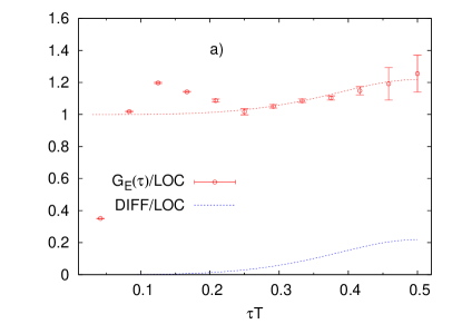
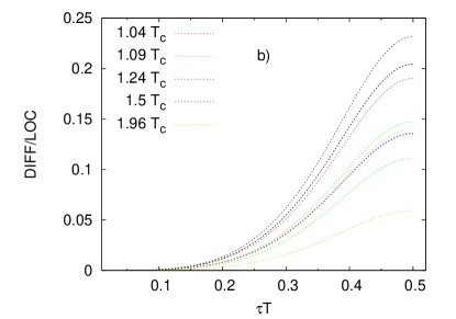
Figure 1: (a) $G_{E}(\tau)$ and the correlator reconstructed from the diffusive part(DIFF), shown normalized to that reconstructed from the leading order part (LOC), at 1.5 $T_{c}$ ($\beta$ = 7.192); see text. (b) The contribution of the diffusive part, normalized by the leading order part, at the different temperatures in Table 1.

In Fig. 1 b) we show the ratio of the diffusive and the leading order parts of the correlator with varying $\tau$ at the different temperatures studied in Table 1. Here we show the 1-$\sigma$ bands and not the best fit values. At all temperatures, except the one at the highest temperature, the diffusive part is seen to reach about 5 % level by $\tau T\sim 0.3$. Note that the accuracy of our correlator is better than this. Also no significant trend of temperature dependence is seen in this figure, indicating the lack of a strong temperature dependence of $\kappa$ in this temperature range.

The value of the momentum diffusion coefficient, $\kappa$, obtained from the analysis outlined above, is shown in Fig. 2 a). The central error bar corresponds to the purely statistical error, obtained from a Jackknife analysis. The larger error bar corresponds to uncertainties due to various systematics:

• As mentioned above, for the central value shown in the figure, we have set $\Lambda=3T$. In order to look for the dependence of the result on this choice, we have varied $\Lambda$ in the range $[2T,\infty)$. A systematic error band which envelops the central values of the fits with varying $\Lambda$ is introduced.

• The fit form, Eq. (9), is a simple model, taking into account the leading order perturbative behavior and the fact that at small $\omega$, $\rho(\omega)\propto\omega$. In order to test the dependence of the extracted value of $\kappa$ on Eq. (9) we also use an alternate form for the infrared part of $\rho(\omega)$:

  $$\rho_{2}(\omega)\;=\;\kappa\>\tanh\frac{\omega}{2T}\;\Theta(\omega-\Lambda)\;+\;b\omega^{3}.$$ (10)

  This form is motivated by classical lattice gauge theory [12]. The difference between $\kappa$ obtained from uses of Eq. (9) and Eq. (10) is also included in the systematic error.

• For the central values in Fig. 2, we have used the range $\tau_{\rm min}$ to $N_{\tau}/2$, where $\tau_{\rm min}$ is the smallest $\tau$ for which we got a good $\chi^{2}$. We looked for the stability of the fit values for variation of $\tau_{\rm min}$. In all sets except one, we could get stable fits, with good $\chi^{2}$ for $\tau_{\rm min}\geq N_{\tau}/4$. For the set at 1.96 $T_{c}$, where the fit value was not so stable, we included the variation of the fit value into our systematic error estimation.

A detailed discussion of the sizes of the various systematics can be found in Ref. [6]. Within the small variation of $LT$ our resources permitted, we did not find a finite volume dependence above our other errors for $LT\geq 2$.

The value of $\kappa/T^{3}$ at 1.5 $T_{c}$, shown in Fig. 2 a), agrees within errors with a similar calculation by Francis et al. [13], while an earlier calculation [14] found smaller values. It is also an order-of-magnitude larger than the LO perturbation theory value that can be extracted from Ref. [2].

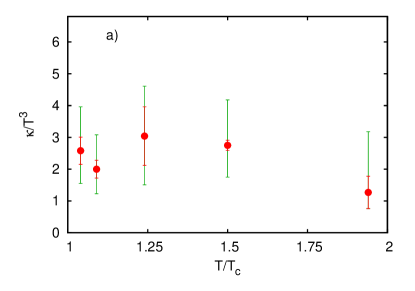
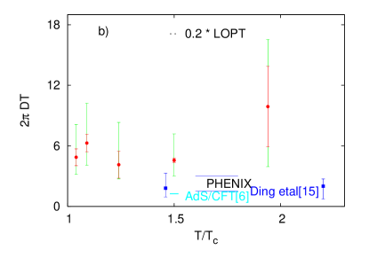
Figure 2: (a) $\kappa/T^{3}$ extracted from $G_{E}(\tau)$, as explained in the text, at various temperatures in the gluon plasma. (b) The diffusion coefficient, $D$, obtained from $\kappa$ using Eq. (11). Also shown are the LO perturbation theory estimate [2] and a different lattice estimate [15], both for gluon plasma. The experimental value quoted by PHENIX, and an estimate from the $\mathcal{N}=4$ supersymmetric Yang-Mills theory are also shown.

The experimental results for heavy quark diffusion are usually presented in terms of the diffusion coefficient $D$, which controls diffusion of the heavy quark in position space. The Einstein relation,

$$D=\frac{T}{M\eta_{D}}=\frac{2T^{2}}{\kappa},$$ (11)

connects $D$ with $\kappa$. $D$ obtained from Eq. (11) and Fig. 2 a) is shown in Fig. 2 b). The leading order perturbation theory value [2] is also shown there.

A more direct approach to calculating $D$ from lattice QCD would be to look at the correlation function of the heavy quark number current, $\bar{Q}\gamma_{i}Q$. A calculation of $D$ for the gluon plasma using such an approach has been presented in Ref. [15]. Their results are also shown in Fig. 2 b), where we have added there statistical and systematic errors in quadrature. The results are even further from the perturbation theory estimate and systematically lower than our results, although consistent within the large error bars.

Our results are for a gluon plasma, so a comparison with the experimental results [4] requires due caution. At the least, a comparison of the results in Fig. 2 with the perturbative results for quenched QCD gives us an indication of how much the nonperturbative results can change from the perturbative results in the deconfined plasma at moderate temperatures $<2T_{c}$. Even then, the results are most encouraging since they indicate that the nonperturbative estimate for $DT$ can easily be an order of magnitude lower than perturbation theory, bringing it in the right ballpark to explain the $v_{2}$ data.

Since dimensionless ratios of various quantities are known to scale nicely between quenched and full QCD if plotted as function of $T/T_{c}$, one can, more optimistically, hope that our results, as plotted in Fig. 2, will be even quantitatively close to the full QCD values. In this spirit, in Fig. 2 b) we also compare the lattice results with the experimental data. The lattice results seem to be a little above the best range for description of the PHENIX data [4] using the Langevin approach [2], though reasonably close within our large systematics. Interestingly, our lattice results seem to show very little temperature dependence in the temperature regime studied here.

As mentioned in Sec. 1, the heavy quark diffusion coefficient has also been calculated in a very different theory, the $\mathcal{N}=4$ supersymmetric Yang-Mills theory with the number of colors, $N_{c}\to\infty$, at large ’t Hooft coupling $\lambda_{tH}=g^{2}N_{c}$, using AdS/CFT correspondence [8]. Of course, this theory is very different from QCD in many respects. Moreover, it crucially exploits symmetries which QCD does not have. However, to get a feel for what kind of values of $D$ such a theory would predict for parameters relevant for QCD at $\sim 1.5T_{c}$, we naively set $N_{c}=3$ and $\alpha_{S}$ = 0.23 in the results of Ref. [8]. This gives $DT\simeq 0.2$ (Fig. 2 b), which is lower than, but in the same ballpark as our estimate.

References

- [1] B. Svetitsky, Phys. Rev.D 37 (1988) 2484.
- [2] G. D. Moore and D. Teaney, Phys. Rev.C 71 (2005) 064904.
- [3] J. Kapusta and C. Gale, Finite Temperature Field Theory, Cambridge University Press.
-
[4]
A. Adare et al.. (PHENIX Collab.), Phys. Rev. Lett.98 (2007) 172301. Phys. Rev.C 84 (2011) 044905.
B.I. Abelev et al.. (STAR Collab.), Phys. Rev. Lett.98 (2007) 192301. - [5] S. Caron-Huot and G. Moore, J. H. E. P. 0802 (2008) 081.
- [6] D. Banerjee, S. Datta, R. Gavai and P. Majumdar, Phys. Rev.D 85 (2012) 014510.
- [7] H. B. Meyer, Eur.Phys.J. A47 (2011) 86.
- [8] J. Casalderrey-Solana and D. Teaney, Phys. Rev.D 74 (2006) 085012.
- [9] S. Caron-Huot, M. Laine and G. D. Moore, J. H. E. P. 0904 (2009) 053.
- [10] M. Lüscher and P. Weisz, J. H. E. P. 0109 (2001) 010, J. H. E. P. 0207 (2002) 049.
- [11] G. P. Lepage and P. Mackenzie, Phys. Rev.D 48 (1993) 2250.
- [12] M. Laine, G. Moore, O. Philipsen and M. Tassler, J. H. E. P. 0905 (2009) 014.
- [13] A. Francis, O. Kaczmarek, M. Laine and J. Langelage, PoS LATTICE2011 (2011) 202.
- [14] H. B. Meyer, New J. Phys. 13 (2011) 035008.
- [15] H. T. Ding et al.., Phys. Rev.D 86 (2012) 014509.