Helicity conservation in nonlinear mean-field solar dynamo

Abstract

We explore the impact of magnetic helicity conservation on the mean-field solar dynamo using the axisymmetric dynamo model which includes the subsurface shear. Our results support the recent findings by Hubbard & Brandenburg (2012), who suggested that the catastrophic quenching in the mean-field dynamo is alleviated if conservation of the total magnetic helicity is taken into account. We show that the solar dynamo can operate in the wide rage of the magnetic Reynolds number up to $10^{6}$. We also found that the boundary conditions for the magnetic helicity influence the distribution of the $\alpha$-effect near the solar surface.

Keywords: Turbulence: Mean-field magnetohydrodynamics; Sun: magnetic field; Stars: activity – Dynamo

I Introduction

The basic idea for the solar dynamo action was developed by Parker (1955). He suggested that the toroidal component of the magnetic field of the Sun is stretched from the poloidal component by the differential rotation ($\Omega$ effect) and the cyclonic motions ($\alpha$ effect) return the part of the toroidal magnetic field energy back to the poloidal component. This is the so-called $\alpha\Omega$ scenario. This mechanism is implemented in the wide range of the solar dynamo models (see review by Charbonneau, 2005).

The effect of the turbulence in the mean-field dynamo is represented by the mean electromotive force $\boldsymbol{\mathcal{E}}\mathbf{=}\overline{\mathbf{u}\times\mathbf{b}}$, where $\mathbf{u}$ and $\mathbf{b}$ are the fluctuating velocity and magnetic fields. In the simplest case it can be found that $\boldsymbol{\mathcal{E}}=\alpha_{0}\overline{\mathbf{B}}+\left(\mathbf{\overline{V}}^{(p)}\times\overline{\mathbf{B}}\right)-\eta_{T}\left(\nabla\times\overline{\mathbf{B}}\right),$ where $\alpha_{0}$ is the $\alpha$ effect, $\mathbf{\overline{V}}^{(p)}$ is the turbulent pumping and $\eta_{T}$ is the turbulent diffusivity (Krause & Rädler, 1980). The $\alpha$ effect is a pseudo-scalar (lacks the mirror symmetry) which is related to the kinetic helicity of the small-scale flows, i.e., ${\displaystyle\alpha_{0}=-\frac{\tau_{c}}{3}\overline{\mathbf{u}\cdot\boldsymbol{\nabla\times}\mathbf{u}}}$, where $\tau_{c}$ is correlation time of turbulent motion. Pouquet et al. (1975) showed that the $\alpha$ effect is produced not only by kinetic helicity but also by current helicity, and it is ${\displaystyle\alpha_{0}=-\frac{\tau_{c}}{3}\left(\overline{\mathbf{u}\cdot\boldsymbol{\nabla\times}\mathbf{u}}-\frac{\mathbf{\overline{b\cdot\boldsymbol{\nabla\times b}}}}{2\mu\overline{\rho}}\right)}$. The latter effect can be interpreted as resistance of magnetic fields against to the twist by helical motions. It leads to the concept of the catastrophic quenching of the $\alpha$ effect by the generated large-scale magnetic field. It was found that ${\displaystyle\alpha_{0}\left(\overline{B}\right)=\frac{\alpha_{0}\left(0\right)}{1+R_{m}\left(\overline{B}/\overline{B}_{eq}\right)^{2}}}$, where $R_{m}$ is magnetic Reynolds number (see, Kleeorin & Rogachevskii, 1999 and references therein). In case of $R_{m}\gg 1$, the $\alpha$ effect is quickly saturated for the large-scale magnetic field strength that is much below the equipartition value ${\displaystyle\overline{B}_{eq}\sim\sqrt{\overline{\rho}\mu_{0}\overline{u^{2}}}}$. The result was confirmed by the direct numerical simulations (DNS) (Ossendrijver et al., 2001). The catastrophic quenching (CQ) is related to the dynamical quenching of the $\alpha$ effect. It is based on conservation of the magnetic helicity, $\overline{\chi}=\overline{\mathbf{a\cdot}\mathbf{b}}$ ($\mathbf{a}$ is fluctuating part of the vector potential) and the relation between the current and magnetic helicities $h_{\mathcal{C}}=\mathbf{\overline{b\cdot\boldsymbol{\nabla\times b}}\sim\overline{\chi}}/\ell^{2}$, which is valid for the isotropic turbulence(Moffatt, 1978). The evolution equation for $\overline{\chi}$ can be obtained from equations that govern $\mathbf{a}$ and $\mathbf{b}$, it reads as follows (Kleeorin & Rogachevskii, 1999):

$$\frac{\partial\overline{\chi}}{\partial t} = -2\left(\boldsymbol{\mathcal{E}}\cdot\overline{\bm{B}}\right)-\frac{\overline{\chi}}{R_{m}\tau_{c}}-\boldsymbol{\nabla}\cdot\boldsymbol{\boldsymbol{\mathcal{F}}}^{\chi}-\eta\overline{\mathbf{B}}\cdot\mathbf{\overline{J}},$$ (1)

where, in following to Kleeorin & Rogachevskii (1999), we introduce the helicity fluxes $\boldsymbol{\boldsymbol{\mathcal{F}}}^{\chi}=\mathbf{\overline{a\times u}}\times\mathbf{B}-\mathbf{\overline{a\times(u\times b)}}$. The helicity fluxes are capable to alleviate the catastrophic quenching (see, e.g., Brandenburg & Subramanian, 2005; Vishniac & Cho, 2001 and references therein). Generally, it was found that the diffusive fluxes, which are $\sim\eta_{\chi}\boldsymbol{\nabla}\overline{\chi}$, where $\eta_{\chi}$ is the turbulent diffusivity of the magnetic helicity, work robustly in the mean-field dynamo models but it requires $\eta_{\chi}>\eta_{T}$ to reach $\left|\overline{B}\right|\geq 0.1\overline{B}_{eq}$.

Another possibility to alleviate the catastrophic quenching is related with the non-local formulation of the mean-electromotive force (Brandenburg et al., 2008). In fact, the Babcock-Leighton (BL) type dynamo is the the special case of the mean-field dynamo with the nonlocal $\alpha$ effect. Kitchatinov & Olemskoy (2011) found that the nonlocal $\alpha$ effect and the diamagnetic pumping can alleviate the catastrophic quenching. The results by Brandenburg & Käpylä (2007) show that the strength of the quenching can depend on the model design. Therefore, the problem of the catastrophic quenching is actual for different types of the solar dynamo.

Recently, Hubbard & Brandenburg (2012) revisited the concept of catastrophic quenching and showed that for the shearing dynamos the Eq.(1) produces the nonphysical fluxes of the magnetic helicity over the spatial scales. They suggested to cure the problem using the global conservation law for the total magnetic helicity that can be written as follows:

$$\frac{d}{dt}\int\left\{\overline{\chi}+\overline{\mathbf{A}}\cdot\overline{\mathbf{B}}\right\}dV = -\eta\int\left\{\overline{\mathbf{B}}\cdot\mathbf{\overline{J}}+\overline{\mathbf{b\cdot j}}\right\}dV$$

$$-\int\boldsymbol{\nabla\cdot}\boldsymbol{\boldsymbol{\mathcal{F}}}^{\chi}dV$$

where integration is done over the volume that comprises the ensemble of the small-scale fields. We assume that $\boldsymbol{\boldsymbol{\mathcal{F}}}^{\chi}$ is the diffusive flux of the total helicity which is resulted from the turbulent motions. Ignoring the effect of the meridional circulation we write the local version of the Eq.(I) as follows (Hubbard & Brandenburg, 2012):

$$\frac{\partial\overline{\chi}}{\partial t}=-\frac{\partial\left(\overline{\mathbf{A}}\cdot\overline{\mathbf{B}}\right)}{\partial t}-\frac{\overline{\chi}}{R_{m}\tau_{c}}-\eta\overline{\mathbf{B}}\cdot\mathbf{\overline{J}}-\boldsymbol{\nabla\cdot}\boldsymbol{\boldsymbol{\mathcal{F}}}^{\chi},$$ (3)

where ${\boldsymbol{\mathcal{F}}}^{\chi}=-\eta_{\chi}\boldsymbol{\nabla}\left(\overline{\chi}+\overline{\mathbf{A}}\cdot\overline{\mathbf{B}}\right)$. In the paper we employ this equation for the dynamical quenching of the $\alpha$ effect in the solar dynamo model and show how it works in the range of the magnetic Reynolds number $R_{m}=10^{3-6}$ those are typical for the astrophysical conditions.

II Basic equations

We study the mean-field induction equation in a perfectly conducting medium:

$$\frac{\partial\overline{\bm{B}}}{\partial t}=\boldsymbol{\nabla}\times\left(\boldsymbol{\mathcal{E}}+\overline{\bm{U}}\times\overline{\bm{B}}\right),$$ (4)

where $\boldsymbol{\mathcal{E}}=\overline{\bm{u\times b}}$ is the mean electromotive force, with $\bm{u,\,b}$ being fluctuating velocity and magnetic field, respectively, $\overline{\bm{U}}$ is the mean velocity (differential rotation), and the axisymmetric magnetic field is:

$$\overline{\bm{B}}=\bm{e}_{\phi}B+\nabla\times\frac{A\bm{e}_{\phi}}{r\sin\theta},$$

where $\theta$ is the polar angle. The mean electromotive force $\boldsymbol{\mathcal{E}}$ is given by Pipin (2008). It is expressed as follows:

$$\mathcal{E}_{i}=\left(\alpha_{ij}+\gamma_{ij}^{(\Lambda)}\right)\overline{B}_{j}-\eta_{ijk}\nabla_{j}\overline{B}_{k}.$$ (5)

The tensor $\alpha_{ij}$ represents the $\alpha$-effect, $\gamma_{ij}^{(\Lambda)}$ is the turbulent pumping, and $\eta_{ijk}$ is the diffusivity tensor. The $\alpha$ effect includes hydrodynamic and magnetic helicity contributions,

$$\alpha_{ij} = C_{\alpha}\sin^{2}\theta\alpha_{ij}^{(H)}+\alpha_{ij}^{(M)}$$ (6)

The details in expressions for the kinetic part of the $\alpha$ effect $\alpha_{ij}^{(H)}$, as well as $\gamma_{ij}^{(\Lambda)}$ and $\eta_{ijk}$ can be found in (Pipin et al., 2012). The contribution of small-scale magnetic helicity $\overline{\chi}=\overline{\bm{a\cdot}\bm{b}}$ ($\bm{a}$ is the fluctuating vector-potential of the magnetic field) to the $\alpha$-effect is defined as

$$\alpha_{ij}^{(M)}=2f_{2}^{(a)}\delta_{ij}\frac{\overline{\chi}\tau_{c}}{\mu_{0}\overline{\rho}\ell^{2}}-2f_{1}^{(a)}e_{i}e_{j}\frac{\overline{\chi}\tau_{c}}{\mu_{0}\overline{\rho}\ell^{2}}.$$ (7)

The nonlinear feedback of the large-scale magnetic field to the $\alpha$-effect is described by a dynamical quenching due to the constraint of magnetic helicity conservation given by Eq.(3). The effect of turbulent diffusivity, which is anisotropic due to the Coriolis force, is given by:

$$\eta_{ijk} = 3\eta_{T}\left\{\left(2f_{1}^{(a)}-f_{2}^{(d)}\right)\varepsilon_{ijk}-2f_{1}^{(a)}e_{i}e_{n}\varepsilon_{njk}\right.$$

$$\left.+C_{\delta}f_{4}^{(d)}e_{j}\delta_{ik}\right\},$$

where functions $f_{\{1,2,4\}}^{(a,d)}$ depend on the Coriolis number. They can be found in Pipin (2008). The last part of Eq. (II) stands for the $\Omega\times J$ effect (Rädler, 1969). The DNS dynamo experiments support the existence of the dynamo effects induced by the large-scale current and global rotation (Käpylä et al., 2008; Schrinner, 2011).

We matched the potential field outside and the perfect conductivity at the bottom boundary with the standard boundary conditions. For the magnetic helicity we employ $\bar{\chi}=0$ at the bottom of the convection zone. At the top we use two types of the boundary conditions like

$$\nabla_{r}\bar{\chi} = 0,$$ (9)

$$\nabla_{r}\left(\bar{\chi}+\overline{\mathbf{A}}\cdot\overline{\mathbf{B}}\right) = 0.$$ (10)

To evolve the Eq.(3) we have to define the large-scale vector potential for each time-step. For the axisymmetric large-scale magnetic fields where the vector-potential is $\overline{\mathbf{A}}=\mathbf{e}_{\phi}A/\left(r\sin\theta\right)+r\mathbf{e}_{r}T$. The toroidal part of the vector potential is governed by the dynamo equations. The poloidal part of the vector potential can be restored from equation $\boldsymbol{\nabla}\times\left(\mathbf{r}T\right)=\mathbf{e}_{\phi}B$. The restoration procedure is trivial for the pseudo-spectral numerical schemes which are based on the Legendre polynomial decomposition for the latitude profile of the large-scale toroidal field.

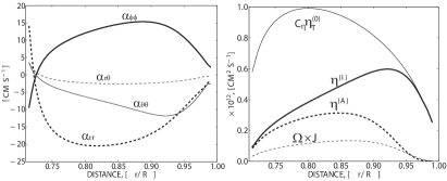
Figure 1: Left, (a), the profiles of the $\alpha$ effects components for the $\theta=45^{\circ}$. Right, (b), the profiles of the background turbulent diffusivity $C_{\eta}\eta_{T}$, the isotropic, $\eta^{(I)}$, and anisotropic, $\eta^{(A)}$, parts of the magnetic diffusivity and $\Omega\times J$ effect (also known as $\delta$ effect (Rädler, 1969).

The choice of parameters in the dynamo is justified by our previous studies (Pipin & Kosovichev, 2011a). Here we use $C_{\alpha}=0.03$, $C_{\delta}=\frac{1}{3}C_{\alpha}$ and the diffusivity dilution factor $C_{\eta}=0.1$. The parameters of the models are summarized in the Table 1.

Table 1: Summary of parameters of the models. Here, QT stands for the quenching type and BC - the boundary conditions.

Model	QT11, QT21	QT12,3	QT22,3
$R_{\chi}$	$10^{6}$	$10^{3}$,$10^{5}$	$10^{3}$,$10^{5}$
QT	Eq. (III) ,Eq. (3)	Eq. (3)	Eq. (1)
$\eta_{\chi}$	$10^{-5}\eta_{T}$	$10^{-2}\eta_{T}$	$10^{-2}\eta_{T}$
BC	Eq. (9)	Eq. (9)	Eq. (9),Eq. (10)

We estimate the turbulent parameters in the model on the base of the mixing-length theory and use as the reference the solar interior model computed by Stix (2002). The differential rotation profile is like that suggested by Pipin & Kosovichev (2011c). Fig. 1 shows the radial profiles of the $\alpha$ effect components and profiles of the background turbulent diffusivity $C_{\eta}\eta_{T}$, the isotropic, $\eta^{(I)}$, and anisotropic, $\eta^{(A)}$, parts of the magnetic diffusivity as well as profile for the $\Omega\times J$ effect.

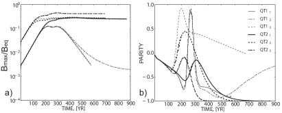
Figure 2: Left panel (a) shows the ratio of the maxima of the toroidal magnetic field strength and the equipartition value with time; (b) shows the parity indexes evolution in the models. We employ the running average to filter out the separate cycles.

To quantify the mirror symmetry type of the toroidal magnetic field distribution relative to equator we introduce the parity index $P$:

$$P = \frac{E_{q}-E_{d}}{E_{q}+E_{d}},$$

$$E_{d} = \int\left(B\left(r_{0},\theta\right)-B\left(r_{0},\pi-\theta\right)\right)^{2}\sin\theta d\theta,$$

$$E_{q} = \int\left(B\left(r_{0},\theta\right)+B\left(r_{0},\pi-\theta\right)\right)^{2}\sin\theta d\theta,$$

where $E_{d}$ and $E_{q}$ are the energies of the dipole-like and quadruple-like modes, $r_{0}=0.9R_{\odot}$. We define the dynamical quenching type 1 (QT1) to be govern by Eq.(1), and the dynamical quenching type 2 (QT2) - by Eq. (3).

III Results

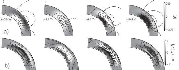
Figure 3: Snapshots of the magnetic field and helicity evolution inside the North segment of the convection zone for the model QT2₃. Panel (a) shows the field lines of the poloidal component of the mean magnetic field and the toroidal magnetic field (varies $\pm 700$G) by gray scale density plot. The bottom panel, (b), shows the large-scale (density plot) and small-scale magnetic helicity (contours) distributions. Both kinds of the magnetic helicity vary in the same range of magnitude.

Fig. 2 shows the long-term evolution of the maximum of the large-scale magnetic field strength in the convection zone and the parity in the models. The energy of the toroidal magnetic fields in all models show the exponential grow in the beginning phase, which has duration about 10 diffusive time of the system. The greater initial magnetic field strength, the shorter duration of the exponential grow phase. Two models QT1₁ and QT2₁ have rather small diffusive fluxes of the helicity and the high magnetic Reynolds number $R_{m}=10^{6}$. We consider them as the references. It is shown below, see Figures 2 and 4 that the model QT2₁ is not subjected to the catastrophic quenching while the model QT1₁ saturates the toroidal magnetic field strength to the level that is much below the equipartition. The moderate diffusive flux with $\eta_{\chi}=0.01\eta_{T}$ (model QT1₃) does not alleviate the problem if the magnetic helicity evolution is governed by the Eq. (1). In the models QT1₂ and QT2_1,3 the saturation level of the toroidal magnetic field strength is about $0.3B_{{\rm eq}}$, where $B_{{\rm eq}}$ is the equipartition level of the magnetic field strength. It is about $0.5B_{eq}$ in the model QT2₂ which has $R_{m}=10^{3}$. The saturation level in the QT2 types solar dynamo can be higher for the the greater $C_{\alpha}$. This question needs a separate study. In the model QT1₁ as well as in all the QT2 models the parity index saturates to the dipole-like solution. In the QT1_2,3 models the asymptotic stage is not clear and they need much longer runs.

The origin of difference in behaviour of the magnetic helicity evolution in the models with QT1 and QT2 has been discussed recently by Hubbard & Brandenburg (2012). Taking into the dynamo equation (4), the corresponding equation for the large-scale vector potential:

$$\frac{\partial\overline{\mathbf{A}}}{\partial t} = \boldsymbol{\mathcal{E}}+\overline{\mathbf{U}}\times\overline{\mathbf{B}},$$ (11)

where we assume the Coulomb gauge, we find the equation which governs the large-scale helicity evolution:

$$\frac{\partial\left(\overline{\mathbf{A}}\cdot\overline{\mathbf{B}}\right)}{\partial t}\!\! = \!\!2\boldsymbol{\mathcal{E}}\cdot\overline{\mathbf{B}}\!\!+\!\!\boldsymbol{\nabla}\cdot\left(\left(\boldsymbol{\mathcal{E}}\times\overline{\mathbf{A}}\right)\!\!-\!\!\mathbf{\overline{A}}\times\left(\overline{\mathbf{U}}\times\overline{\mathbf{B}}\right)\right).$$ (12)

Therefore, Eq. (3) can be rewritten in form of Eq.(I):

$$\frac{\partial\overline{\chi}}{\partial t} = -2\left(\boldsymbol{\mathcal{E}}\cdot\overline{\bm{B}}\right)-\frac{\overline{\chi}}{R_{m}\tau_{c}}+\boldsymbol{\nabla}\cdot\left(\eta_{\chi}\boldsymbol{\nabla}\bar{\chi}\right)$$

$$-\eta\overline{\mathbf{B}}\cdot\mathbf{\overline{J}}-\boldsymbol{\nabla}\cdot\left(\boldsymbol{\mathcal{E}}\times\overline{\mathbf{A}}\right).$$

The term $\left(\boldsymbol{\mathcal{E}}\times\overline{\mathbf{A}}\right)$ consists of the counterparts of the sources magnetic helicity, which are represented by $-2\boldsymbol{\mathcal{E}}\cdot\overline{\mathbf{B}}$, and the fluxes which result from pumping of the large-scale magnetic fields. The sources magnetic helicity in the term $-2\left(\boldsymbol{\mathcal{E}}\cdot\overline{\bm{B}}\right)$ are partly compensated in Eq(III) by the counterparts in $\left(\boldsymbol{\mathcal{E}}\times\overline{\mathbf{A}}\right)$. This results in the spatially homogeneous quenching of the large-scale magnetic generation and alleviation of the catastrophic quenching problem. The last term in Eq(12) contains the transport of the large-scale magnetic helicity by the large-scale flow.

Fig. 3 shows the snapshots of the magnetic field and magnetic helicity (large- and small-scale) evolution in the North segment of the solar convection zone for the model QT2₃. We observe the drift of the dynamo waves which are related to the large-scale toroidal and poloidal fields towards the equator and towards the pole, respectively. The distributions of the large- and small-scale magnetic helicities show the correspondence in sign: positive to negative, and the other way around, respectively. This is in agreement with Eq. (3). It is seen that the negative sign of the magnetic helicity follows the dynamo wave of the toroidal magnetic field. This can be related to the so-called “current helicity hemispheric sign rule” (negative/positive sign of helicity dominate in the North/South hemisphere) which is suggested by the observations (see Seehafer (1990); Zhang et al. (2010) and references therein). The origin of the helicity sign rule has been extensively studied in the dynamo theory (e.g., Choudhuri et al., 2004; Zhang et al., 2012). The similar snapshots for the QT1 model can be found in (Pipin & Kosovichev, 2011b). The main difference is that for the QT1 model all the changes in the magnetic helicity evolution does not exactly follow to the dynamo wave inside the convection zone as it is demonstrated for the QT2 model.

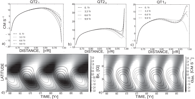
Figure 4: First row, (a,b and c), shows variations of the $\alpha$ effect ($\alpha_{\phi\phi}$ component) profiles with the cycle at colatitude $\theta=45^{\circ}$, for the model QT2₁, QT2₃ and QT1₂ (from left to right). The bottom, panel (d) shows the time - latitude variations of the toroidal field near the surface, $r=0.95R_{\odot}$, (contours $\pm 300$G) and the radial magnetic field at the surface (density plot) for the model QT2₃; panel (e) shows the same for the the toroidal field and the $\alpha$ effect ($\alpha_{\phi\phi}$ component)(density plot).

Fig. 4 shows variations of the radial profiles of the $\alpha$ effect and magnetic helicity with the cycle and the time-latitude diagrams for the dynamo model QT2₃. For all the models the changes in the $\alpha$ effect are concentrated to the top of the convection zone. This is due to the factor $\left(\overline{\rho}\ell^{2}\right)^{-1}$ in relation between the current and magnetic helicities. The difference in the boundary at the top results in different distributions of the $\alpha$ effect in the models QT2₁ and QT2₃. We would like to notice that the QT1₂ and QT2₁ have the same boundary conditions, however, the resulted distributions of the $\alpha$ effect differ drastically. The time-latitude diagrams for the dynamo model QT2₃ which are shown in Figure 4, are in qualitative agreement with observations. The same patterns are obtained in the models QT2_1,2. We show the dynamical $\alpha$ effect as well. The model shows that with the boundary conditions given by Eq. (10) the $\alpha$ effect increases and has positive maxima at the growing phase of the cycle and it decreases, having the negative minima at the decaying phase of the cycle.

IV Conclusion

In the paper we studied the effect of the magnetic helicity conservation in the mean-field solar dynamo model which is shaped by the subsurface shear. The results show that the solar dynamo can operate in the wide rage of the magnetic Reynolds number up to $10^{6}$ if conservation of the total magnetic helicity is taken into account.

It was found that the boundary conditions for the magnetic helicity influence the distribution of the $\alpha$ effect near the solar surface. For example, the dynamo wave becomes closer to equator when the diffusive flux of the total helicity is zero at the top of the convection zone because the dynamical increase of the $\alpha$ effect follows the dynamo wave (see Fig. 3, 4). The situation is opposite for the case when the diffusive flux is dominated by the large-scale helicity. Thus, the parity breaking in the solar dynamo can occur due to perturbations in the external boundary for the magnetic helicity. However, these points remain an open field for the future work.