Quantum crystal growing: Adiabatic preparation of a bosonic antiferromagnet in the presence of a parabolic inhomogeneity

Abstract

We theoretically study the adiabatic preparation of an antiferromagnetic phase in a mixed Mott insulator of two bosonic atom species in a one-dimensional optical lattice. In such a system one can engineer a tunable parabolic inhomogeneity by controlling the difference of the trapping potentials felt by the two species. Using numerical simulations we predict that a finite parabolic potential can assist the adiabatic preparation of the antiferromagnet. The optimal strength of the parabolic inhomogeneity depends sensitively on the number imbalance between the two species. We also find that during the preparation finite size effects will play a crucial role for a system of realistic size. The experiment that we propose can be realized, for example, using atomic mixtures of Rubidium 87 with Potassium 41 or Ytterbium 168 with Ytterbium 174.

1 Introduction

The hardware of an (analog) quantum simulator [1] is a controlled quantum system that is a clean and tunable realization of a many-body model system of interest (see also Refs. [2, 3]). In a quantum simulation such a quantum machine is used to experimentally measure dynamical or equilibrium properties of the model that are hard to obtain by using a classical machine. A typical protocol for studying equilibrium properties will start from a parameter regime of the model that is well understood theoretically and, thus, allows validating that a state close to thermal equilibrium can be prepared faithfully. In a next step, the system is then guided slowly into the parameter regime of interest. If it can be assumed that the dynamics during this parameter variation is close to adiabatic, the system will finally be in a state close to the target state, which is defined to be the thermal equilibrium for the new set of parameters characterized, e.g., by the same entropy and particle number as the initial state.

However, typically a phase transition is expected to occur on the way between the initial and the target regime. Crossing this transition is potentially a source for an increased production of excitations as described by the Kibble-Zurek mechanism in the case of a continuous phase transition (see Refs. [4, 5] and References therein). In order to keep defect creation at a minimal level, it has been proposed to bring the system from one quantum phase to the other without passing a true phase transition by employing spatial inhomogeneity [6, 7, 8]. Namely, in an inhomogeneous system the transition from one phase to another can happen as a crossover at a spatial boundary of finite width. By parameter variation this boundary can be moved through the system at a finite speed, eventually bringing it from one phase to the other. Such a strategy is similar to methods like growing crystals or pulling them out of the melt. It has been investigated theoretically in the simple model system of a quantum spin-1/2 chain (with Ising or XY coupling) in an inhomogeneous transverse field; here the ferromagnet-to-paramagnet transition (a continuous phase transition in the uniform system) can be induced practically without defect creation, provided the phase boundary moves slow enough [7, 8].

In this paper we investigate theoretically a problem of direct experimental relevance. Namely whether a parabolic inhomogeneity can be useful to assist the adiabatic preparation of an antiferromagnetic quantum phase in an experiment with ultra cold atoms [9, 10]. The antiferromagnetic crystalline order shall be grown in space from the center of the system outwards. To this end, we consider a two-species mixture of ultra cold bosonic atoms in an optical lattice with strong on-site repulsion (see, e.g., Refs. [11, 12, 13, 14, 15, 16, 17, 18] for the equilibirum properties of such a system). The system can be described by a quantum XXZ-spin-1/2 model [11, 12, 13] and we are interested in the transition from an easy-plane ferromagnetic phase in the spin $xy$ plane to an easy-axis antiferromagnetic phase in $z$ direction. We will concentrate on a one-dimensional system with the dynamics along the perpendicular directions frozen out by a strong transversal confinement.

The motivation for the present work is twofold. First of all, the quantum antiferromagnetically ordered target state is known to be very fragile with respect to thermal fluctuations, because it is stabilized by low-energy superexchange physics only [17] (for antiferromagnetism in ultra cold atoms without superexchange cf. Refs. [19, 20, 21, 22]). This makes its experimental realization challenging. It is, thus, desirable and of immediate relevance for current experimental studies to investigate how the state can be prepared with a minimum of heating. A related problem of great importance is the preparation of the fermionic Heisenberg antiferromagnet being a prerequisite for mimicking the intriguing physics of high-temperature cuprate superconductors [23] with ultra cold atoms [24].

Another motivation lies in the fact that the system we are studying possesses several interesting properties. It allows to experimentally control and (despite of the fact that the particles are always trapped) even switch off completely a parabolic inhomogeneity by tuning the relative trap strength of the two bosonic species [25]. This enables the experimentalist to study the influence of (in)homogeneity in detail also in the laboratory.

The system is also rich and generic enough to give rise to effects that potentially disfavor the usage of inhomogeneity for the purpose of an adiabatic state preparation. For example, mass flow can be a limiting factor, especially if domains of insulating phases appear, acting as barriers that hamper density redistribution, as recently discussed in the context of the inhomogeneous bosonic Mott transition [26, 27]. Another aspect is that the transition can change from a continuous (second order) transition to a discontinuous (first order) transition (see Ref. [28] for the two-dimensional case). The continuous transition occurs without inhomogeneity, whereas the discontinuous transition is relevant for studying the transition with inhomogeneity.

For the related problem of a fermionic Heisenberg antiferromagnet adiabatic protocols based on inhomogeneities that reduce the discrete translational symmetry of the system, have been investigated recently [29, 30].

In this paper, we study the influence of a static parabolic inhomogeneity, while the transition from one quantum phase to the other is induced by varying terms that themselves do not break translational symmetry. Similar scenarios have recently been investigated for temperature-driven phase transitions [31, 32, 33] or for ramps not passing a phase transition [34]. We are not considering a quench of the inhomogeneity itself, as it has been studied for example in Ref. [35]. We note in passing that the dynamics of a harmonically trapped bose-bose mixture in response to a sudden displacement of the trap has recently been investigated theoretically as a probe for different quantum phases in the system [36].

The numerical studies of the one-dimensional system that we present in this paper indicate that a parabolic potential can indeed assist the adiabatic preparation of the antiferromagnetic target state. However, the optimal strength of the inhomogeneity depends in a sensitive way on the imbalance between the two bosonic species; the larger the imbalance the larger the optimal inhomogeneity. Therefore, the possibility to tune the inhomogeneity [25] should be an advantage for preparing the antiferromagnetic order. We also observe that for realistic system sizes the time evolution during the parameter ramp into the antiferromagnetic regime is still governed by finite size effects that go beyond the local-density picture. Namely we find precursing antiferromagnetic correlations already in the ground state of the system outside the antiferromagnetic regime. These are contaminated with imperfections (like kinks) that originate from the inhomogeneity. The imperfect correlations are amplified when the system is ramped into the antiferromagnetic regime. It is difficult for the system to get rid of these imperfections, as it would be required for a perfectly adiabatic time evolution. So we find the best results for parameters giving rise to an initial state with a low degree of imperfections in the precursing antiferromagnetic order.

The paper is organized as follows. The system and the different models describing it are introduced in section 2. The structure of the grand canonical ground state phase diagram is reviewed in section 3, with some details on how the phase diagram has been computed using the Bethe ansatz in appendix A. The protocol for the preparation of the antiferromagnetic state is described in detail and motivated in section 4. The results of our numerical simulation of this protocol are finally presented in section 5, before we conclude in section 6.

2 System and models

We are considering a system of ultra cold atoms given by a mixture of two bosonic species in one spatial dimension (1D) subjected to a steep optical lattice potential. In recent experiments such mixtures have been loaded into optical lattices, among them Potassium (K41) Rubidium (Rb87) mixtures [37] and mixtures of different hyperfine (“spin”) states of Rb87 [38, 39, 40, 41, 42, 43]. Other candidates include mixtures of different Ytterbium-Isotopes [44, 45] that offer a rich variety of scattering properties depending on the selection of isotopes [46]. In the following we consider a two-species system characterized by all-repulsive interactions and with the intraspecies repulsion being strong compared to the interspecies repulsion. Such a system can be realized experimentally by using an Yb168-Yb174 mixture [46] or, alternatively, by taking a K41-Rb87 mixture with the interspecies scattering length tuned small by means of a Feshbach-resonance [47].

The 1D mixture of two bosonic species $s=a,b$ in an optical lattice is described by the Bose-Hubbard Hamiltonian

$$\hat{H}_{\mathrm{BH}} = \sum_{\ell=-\infty}^{\infty}\Big{[}\sum_{s}\Big{\{}-J_{s}(\hat{a}^{{\dagger}}_{s\ell+1}\hat{a}^{\phantom{{\dagger}}}_{s\ell}+\mathrm{h.c.})$$ (1)

$$+\,(V_{s\ell}-\mu_{s})\hat{n}_{s\ell}\Big{\}}+U_{ab}\hat{n}_{a\ell}\hat{n}_{b\ell}$$

$$+\,\frac{U_{aa}}{2}\hat{n}_{a\ell}(\hat{n}_{a\ell}-1)+\frac{U_{bb}}{2}\hat{n}_{b\ell}(\hat{n}_{b\ell}-1)\Big{]},$$

where $\hat{a}^{\phantom{{\dagger}}}_{s\ell}$ and $\hat{n}_{s\ell}$ are the bosonic annihilation and number operator for particles of species $s$ at lattice site $\ell$. Tunneling between neighboring sites is captured by the positive matrix elements $J_{s}$; the three positive Hubbard energies $U_{ab}$, $U_{aa}$, and $U_{bb}$ characterize the repulsive inter and intra species on-site interactions; and the particles are confined by the harmonic trapping potentials $V_{s\ell}=\frac{1}{2}\alpha_{s}\ell^{2}$. In the ground state the total numbers $N_{a}$ and $N_{b}$ of $a$ and $b$ particles are controlled by the chemical potentials $\mu_{s}$.

We are interested in the regime of strong repulsive interactions with the Hubbard energies $U_{s^{\prime}s}$ being positive and large compared to both the tunneling matrix elements $J_{s}$ and the chemical potentials $\mu_{s}$ such that double occupancy is strongly suppressed. Under these conditions we can effectively describe the system within the low-energy subspace $S$ defined by

$$S:\;\hat{n}_{a\ell}+\hat{n}_{b\ell}\leq 1\quad\forall\ell.$$ (2)

We employ degenerate-state perturbation theory [48] up to second order with respect to tunneling processes and obtain the effective Hamiltonian

$$\hat{H}_{\mathrm{eff}} = \sum_{\ell}\sum_{s}\Big{[}(V_{s\ell}-\mu_{s})\hat{n}_{s\ell}-J_{s}\hat{P}_{S}(\hat{a}^{{\dagger}}_{s\ell+1}\hat{a}^{\phantom{{\dagger}}}_{s\ell}+\mathrm{h.c.})\hat{P}_{S}$$ (3)

$$-J\,\hat{a}^{{\dagger}}_{s\ell+1}\hat{a}^{\phantom{{\dagger}}}_{\bar{s}\ell+1}\hat{a}^{{\dagger}}_{\bar{s}\ell}\hat{a}^{\phantom{{\dagger}}}_{s\ell}-\frac{U}{2}\hat{n}_{s\ell+1}\hat{n}_{\bar{s}\ell}\Big{]}$$

acting in $S$. Here the operator $\hat{P}_{S}$ projects into the subspace $S$ and $\bar{s}$ denotes the species opposite to $s$. The first and second term originate from zeroth- and first-order perturbation theory, respectively. The new matrix elements $J$ and $U$ describe second-order superexchange processes. While $J$ quantifies swaps between $a$ and $b$ particles on neighboring sites, $U$ characterizes an attractive nearest-neighbor interaction between $a$ and $b$ particles. These matrix elements stem from perturbative admixtures of Fock states with one site occupied by both an $a$ and a $b$ particle and read

$$J = 2\frac{J_{a}J_{b}}{U_{ab}}$$ (4)

$$U = 2\frac{J_{a}^{2}+J_{b}^{2}}{U_{ab}}.$$ (5)

Furthermore, when deriving $\hat{H}_{\mathrm{eff}}$ two additional approximations have been made for simplicity that both are well justified. The first one is that we neglected second-order terms involving virtual excitations (perturbative admixtures) with two particles of the same species on the same site. The amplitudes of such terms are proportional to $~{}J_{a(b)}^{2}/U_{aa(bb)}$ and are much smaller than the effective matrix elements (4) and (5), since we assume $U_{ab}\ll U_{aa},U_{bb}$. The second simplification consists in neglecting the small potential energy differences between neighboring sites $(V_{s\ell+1}-V_{s\ell})=\alpha_{s}(\ell+1/2)$ that would appear together with $U_{ab}$ in the denominators of the second-order matrix elements (4) and (5). This approximation is well justified for typical slowly varying traps.

For a Yb168-Yb174 mixture with scattering lengths $a_{168-168}=13.33\ \mathrm{nm}$, $a_{174-168}=0.13\ \mathrm{nm}$ and $a_{174-174}=5.55\ \mathrm{nm}$ [46], perpendicular lattice depth $V/E_{r}=50$, transversal lattice depths $V_{a}/E_{r}=16$, $V_{b}/E_{r}=29$ and lattice wave-length $\lambda=532\ \mathrm{nm}$ leads to $J_{a}/U_{ab}\approx 0.12$ and $J_{b}/U_{ab}\approx 0.012$ corresponding approximately to Figure 6(b) and a time-scale $\hslash/U\sim 26\ \mathrm{ms}$.

Concerning the level of approximation, the description of the bosonic system in terms of the effective Hamiltonian (3) is comparable to the $tJ$-model for spin-1/2 fermions on a lattice with strong on-site repulsion [49, 50]. It describes the low energy physics of a doped magnet by combing two elements; the superexchange coupling between the spin (or species) degree of freedom on neighboring occupied sites on the one hand and, on the other hand, the dynamics of the charge (or total density) degree of freedom due to the presence of holes (vacant sites). For fermions the interplay between both is conjectured to give rise to intriguing physics like high-temperature superconductivity in the case of a square lattice [23]. The homogeneous version of the bosonic model (3) has been studied theoretically in Refs. [51, 52, 53] where, e.g., phase separation between hole-rich and hole-free regions is predicted on the square lattice.

For slowly varying traps it is useful to introduce the local chemical potentials $\mu_{s\ell}\equiv\mu_{s}-V_{s\ell}$. For sufficiently large $\mu_{a}$ and $\mu_{b}$ (i.e. for a sufficiently large total particle number $N_{a}+N_{b}$), in an extended region $M$ in the trap center the local chemical potentials will be large enough to strongly suppress the existence of unoccupied sites. (An estimate of the size of $M$ will be given at the end of this section). In this region the particles form a mixed Mott insulator with occupation $\langle\hat{n}_{a}+\hat{n}_{b}\rangle\simeq 1$. The remaining degrees of freedom, namely which site is occupied by which species, can then effectively be described within the subspace $S^{\prime}$ of unit filling,

$$S^{\prime}:\;\hat{n}_{a\ell}+\hat{n}_{\ell}=1\quad\forall\ell\in M.$$ (6)

In $S^{\prime}$ and for $\ell\in M$ the Hamiltonian is again given by $\hat{H}_{\mathrm{eff}}$, but the tunneling terms can now be dropped, giving

$$\hat{H} = \sum_{\ell}\Big{[}-J(\hat{a}^{{\dagger}}_{a\ell+1}\hat{a}^{\phantom{{\dagger}}}_{b\ell+1}\hat{a}^{{\dagger}}_{b\ell}\hat{a}^{\phantom{{\dagger}}}_{a\ell}+\mathrm{h.c.})$$

$$-\,\frac{U}{2}(\hat{n}_{b\ell+1}\hat{n}_{a\ell}+\hat{n}_{a\ell+1}\hat{n}_{b\ell})+\frac{1}{2}(V_{\ell}-\mu)(\hat{n}_{a\ell}-\hat{n}_{b\ell})\Big{]}.$$

We have also omitted the constant terms $\frac{1}{2}(\mu_{a\ell}+\mu_{b\ell})(\hat{n}_{a\ell}+\hat{n}_{b\ell})=\frac{1}{2}(\mu_{a\ell}+\mu_{b\ell})$ and introduced the notation

$$V_{\ell}\equiv V_{a\ell}-V_{b\ell}=\frac{1}{2}(\alpha_{a}-\alpha_{b})\ell^{2}\equiv\frac{1}{2}\alpha\ell^{2}$$ (8)

and

$$\mu\equiv\mu_{a}-\mu_{b}.$$ (9)

The effective Hamiltonian (2) will be the starting point for the remaining sections of this paper.

The inhomogeneity $V_{\ell}$ appearing in $\hat{H}$ is characterized by the difference of the trap frequencies $\alpha=\alpha_{a}-\alpha_{b}$. This can be explained as a consequence of the constraint $\hat{n}_{a\ell}+\hat{n}_{b\ell}=1$; tunneling of an $a$ particle from $\ell$ to $\ell^{\prime}$ has to be combined with the counterflow of a $b$ particle from $\ell^{\prime}$ to $\ell$. In an experiment the degree of inhomogeneity $\alpha$ can be tuned continuously, simply by adjusting the trapping potentials of the two species with respect to each other. In particular, the accessible parameter space contains the homogeneous model with $\alpha=0$ that is realized for equal traps $\alpha_{1}=\alpha_{2}$ [25] (as well as the regime of $\alpha<0$). The fact that this limit can be reached without the model description breaking down is a crucial ingredient of the experiment proposed here.

Apart from the dimensionless inhomogeneity $\alpha/U$, the Hamiltonian $\hat{H}$ describing the simulator region $M$ of our system is characterized by two further dimensionless parameters, namely $J/U=(J_{a}/J_{b}+J_{b}/J_{a})^{-1}$ and $\mu/U$. In an experiment these can be controlled independently by adjusting the ratio of tunneling strengths $J_{a}/J_{b}$ (controlled by the lattice depths for $a$ and $b$ particles) and the imbalance between $a$ and $b$ particles $(N_{a}-N_{b})/(N_{a}+N_{b})$.

It is both instructive and convenient to express the Hamiltonian (2) in terms of composite-particle [54] and spin [13] degrees of freedom. The former description is obtained by introducing composite particles that are hard-core bosons with annihilation operators

$$\hat{b}^{\phantom{{\dagger}}}_{\ell}=\hat{a}^{{\dagger}}_{b\ell}\hat{a}^{\phantom{{\dagger}}}_{a\ell}$$ (10)

and number operators $\hat{n}_{\ell}\equiv\hat{b}^{{\dagger}}_{\ell}\hat{b}^{\phantom{{\dagger}}}_{\ell}$, such that $[\hat{b}^{\phantom{{\dagger}}}_{\ell},\hat{b}^{{\dagger}}_{\ell^{\prime}}]=\delta_{\ell,\ell^{\prime}}(1-2\hat{n}_{\ell})$ and

$$\hat{b}^{\phantom{{\dagger}}}_{\ell}\hat{b}^{\phantom{{\dagger}}}_{\ell}=\hat{b}^{{\dagger}}_{\ell}\hat{b}^{{\dagger}}_{\ell}=0$$ (11)

in $S^{\prime}$. With that $\hat{n}_{\ell}\equiv\hat{b}^{{\dagger}}_{\ell}\hat{b}^{\phantom{{\dagger}}}_{\ell}\leq 1$. In $S^{\prime}$ the composite-particle occupation numbers are equal to those of the $a$ particles, $\hat{n}_{\ell}=\hat{n}_{a\ell}(\hat{n}_{b\ell}+1)=\hat{n}_{a\ell}$, whereas “composite holes” correspond to $b$ particles, $1-\hat{n}_{\ell}=\hat{n}_{b\ell}$. The Hamiltonian (2) can now be re-written like

$$\hat{H} = \sum_{\ell}\Big{[}-J(\hat{b}^{{\dagger}}_{\ell+1}\hat{b}^{\phantom{{\dagger}}}_{\ell}+\mathrm{h.c.})+U\Big{(}\hat{n}_{\ell+1}-\frac{1}{2}\Big{)}\Big{(}\hat{n}_{\ell}-\frac{1}{2}\Big{)}$$ (12)

$$+\,(V_{\ell}-\mu)\Big{(}\hat{n}_{\ell}-\frac{1}{2}\Big{)}\Big{]}.$$

This Hamiltonian describes hard-core bosons in a tunable trapping potential $V_{\ell}$, with hopping matrix element $J$, repulsive nearest neighbor interactions $U$, and chemical potential $\mu$.

A spin-1/2 description is defined by identifying the species $s$ with an internal spin degree of freedom with spin $\uparrow$ ($\downarrow$) for $a$ ($b$) particles. Introducing the vector of Pauli matrices ${\bm{\sigma}}_{s^{\prime}s}$ for this spin degree of freedom, we can define the spin operator at site $\ell$:

$$\hat{\bm{S}}_{\ell}=\frac{1}{2}\sum_{s^{\prime}s}\hat{a}^{{\dagger}}_{s^{\prime}\ell}{\bm{\sigma}}_{s^{\prime}s}\hat{a}^{\phantom{{\dagger}}}_{s\ell}$$ (13)

with components

$$\hat{S}^{x}_{\ell} = \frac{1}{2}(\hat{a}^{{\dagger}}_{a\ell}\hat{a}^{\phantom{{\dagger}}}_{b\ell}+\mathrm{h.c.})$$ (14)

$$\hat{S}^{y}_{\ell} = \frac{1}{2}(\mathrm{i}\hat{a}^{{\dagger}}_{b\ell}\hat{a}^{\phantom{{\dagger}}}_{a\ell}+\mathrm{h.c.})$$ (15)

$$\hat{S}^{z}_{\ell} = \frac{1}{2}(\hat{n}_{a\ell}-\hat{n}_{b\ell}).$$ (16)

In the subspace $S^{\prime}$ these spin operators $\hat{\bm{S}}_{\ell}$ describe a spin-1/2 degree of freedom at every site. In terms of these degrees of freedom the Hamiltonian takes the form

$$\hat{H}=\sum_{\ell}\Big{[}-2J(\hat{S}^{x}_{\ell}\hat{S}^{x}_{\ell+1}+\hat{S}^{y}_{\ell}\hat{S}^{y}_{\ell+1})+U\hat{S}^{z}_{\ell}\hat{S}^{z}_{\ell}+(V_{\ell}-\mu)\hat{S}^{z}_{\ell}\Big{]}$$ (17)

of an XXZ spin chain with ferromagnetic spin coupling $-2J\equiv J_{x}=J_{y}$ in $x$ and $y$ direction, antiferromagnetic Ising coupling $+U\equiv J_{z}$ in $z$ direction, and an inhomogeneous magnetic field $(V_{\ell}-\mu)\equiv h_{\ell}$ in $z$ direction.

In the following we will focus on the central Mott insulator region $M$ described by the Hamiltonian $\hat{H}$. It serves as a simulator for the dynamics described by the model Hamiltonian $\hat{H}$ with tunable parabolic inhomogeneity. Let us briefly estimate the size of the Mott insulator region in the zero-temperature equilibrium state. In the limit of zero tunneling both species fill up the trap such that sites $\ell$ with $|\ell|<(N_{a}+N_{b})/2\equiv\ell_{0}$ are occupied. If $\mu_{s^{*}}$ is the larger of the two chemical potentials $\mu_{a}$ and $\mu_{b}$, and $\alpha_{s^{*}}$ denotes the corresponding trap frequency, one has $\frac{1}{2}\alpha_{s^{*}}\ell_{0}^{2}=\mu_{s^{*}}$. In order to suppress doubly occupied sites near the trap center besides $J_{s}\ll U_{ab}$ also $\mu_{s^{*}}<U_{ab}$ is required. The latter implies that $2\ell_{0}<\sqrt{8U_{ab}/\alpha_{s^{*}}}$.

When finite tunneling is included, the edge of the occupied region will soften. With increasing $|\ell|$, near $|\ell|=\ell_{0}$ the occupation $\langle\hat{n}_{a}+\hat{n}_{b}\rangle$ will drop from 1 to 0 within a crossover region of width $\Delta\ell$. The width $\Delta\ell$ is such that the increase of the trapping potential in the crossover region is of the order of the tunneling matrix element. More precisely, $\partial_{\ell}V_{s\ell}|_{\ell=\ell_{0}}\Delta\ell_{s}=\alpha_{\ell}\ell_{0}\Delta\ell_{s}\sim J_{s}$ gives $\Delta\ell_{s}\sim J_{s}/(\alpha_{s}\ell_{0})$ and one has either $\Delta\ell=\max(\Delta\ell_{a},\Delta\ell_{b})$ if both species can be found near the edge $|\ell|\approx\ell_{0}$ (that is $\mu_{a}\approx\mu_{b}$) or $\Delta\ell=\Delta_{s^{*}}$ if basically only $s^{*}$ particles occupy the edge region (i.e. $\mu_{\bar{s}^{*}}\ll\mu_{s^{*}}$). In the former (more restrictive) case the crossover region $\Delta\ell$ will be small compared to $\ell_{0}$ as long as $J_{s}\ll\alpha_{s}\ell_{0}^{2}\approx 2\mu_{s^{*}}<2U_{ab}$, which has been required already. Therefore, the “simulator region” $M$ has an extent of $L\sim 2\ell_{0}-2\Delta\ell$ that will be of the order of $\ell_{0}$ and it can host an extensive fraction of the particles in the system.

3 Ground state phase diagram of the homogeneous system

Figure 1: Ground-state phase diagram of hard-core bosons in a one-dimensional lattice with nearest-neighbor repulsion $U$ described by the Hamiltonian (12) with $V_{\ell}=0$. Subfigure (b) shows the parameter plane given by the dimensionless chemical potential $\mu/U$ and tunneling parameter $J/U$. Thick solid (dashed) lines indicate continuous (discontinuous) phase transitions. The system possesses a compressible superfluid phase (SF) and three incompressible phases, the vacuum at zero filling (V), the particle-hole reflected vacuum at unit filling (U), and a density-wave insulator at half filling (DW). The color code describes the filling $n$ and clearly indicates the incompressible regions where $\partial n/\partial\mu=0$. The DW insulator is characterized by a long-ranged staggered order in the site occupation, measured by the order parameter $O_{\mathrm{DW}}$ defined in Eq. (18). $O_{\mathrm{DW}}$ is non-zero only in the DW phase, where it depends on $J/U$, as plotted in subfigure (a), but not on $\mu/U$. The sudden jump of $O_{\mathrm{DW}}$ to zero when entering the SF phase renders the DW-to-SF transition discontinuous (though the filling $n$ varies continuously when passing the transition). The only exception occurs at the tip of the lobe-shaped DW domain (located at $\mu/U=0$ and $J/U=1/2$) where the transition is continuous. The different thin curves plotted in (b) indicate the chemical potential $\mu/U$ of finite systems in the local density approximation with $N=31,29,27,25$ particles on $L=61$ sites subjected to a trap of strength $\alpha/U=10^{-3}$. The vertical “system lines” attached to these curves indicate how much the chemical potential drops between the center and the edge of the system according to the local density approximation.

In the central Mott region $M$ the system is described by the Hamiltonian $\hat{H}$ that we expressed in different representations. In the following we will stick to the language of the hard-core boson model (12), unless we explicitly mention the two-species [Eq. (2)] or spin [Eq. (17)] description. For a homogeneous system with $V_{\ell}=0$, the ground state of this model is characterized by two dimensionless parameters, the scaled chemical potential $\mu/U$ and the scaled tunneling matrix element $J/U$, with the nearest-neighbor repulsion $U$ serving as the unit of energy. We have computed the phase diagram of the homogeneous system in the $\mu/U$-$J/U$ plane by employing the Bethe-Ansatz solution developed in Refs. [55, 56, 57]. Details of this solution are given in appendix A. In Fig. 1(b) we plot the zero-temperature phase diagram and the boson filling $n=\frac{1}{L}\sum_{\ell\in M}\langle\hat{n}_{i}\rangle$ with $L=\sum_{\ell\in M}1$ denoting the number of lattice sites in $M$.

The phase diagram shown in Fig. 1(b) possesses the following structure. First of all, it reflects the particle-hole symmetry of the homogeneous hard-core boson model (12); replacing $\hat{b}^{\phantom{{\dagger}}}_{\ell}\to\hat{b}^{{\dagger}}_{\ell}$ [implying $(\hat{n}_{\ell}-1/2)\to(1/2-\hat{n}_{\ell})$] and $\mu\to-\mu$ leaves the Hamiltonian unchanged, such that $\mu\to-\mu$ simply interchanges the role of particles and holes.

The energy of a single particle with respect to the vacuum energy is given by $-\mu-U-2J$ with the kinetic energy reduction $-2J$ stemming from delocalization. Therefore, below a chemical potential of $\mu_{v}/U=-2J/U-1$ the system is in the vacuum (V) state $|v\rangle$ with no particles present. Accordingly, for chemical potentials larger than $\mu_{u}/U=-\mu_{v}/U=2J/U+1$ the ground state is the particle-hole reflected vacuum, that is the incompressible insulating state $|u\rangle=\prod_{\ell}\hat{b}^{{\dagger}}_{\ell}|v\rangle$ at unit filling (U) with exactly one hard-core particle at every site.

Starting from the vacuum state and increasing the chemical potential $\mu/U$, for non-zero tunneling $J/U$ the particle number starts to grow in a continuous fashion once the critical parameter $\mu_{v}/U$ is passed. Here the system enters a superfluid (SF) phase in a second-order phase transition. This phase is characterized by a finite compressibility $\partial_{\mu}n\neq 0$, a homogeneous density distribution $n_{\ell}=\langle\hat{n}_{\ell}\rangle=n$, and quasi-long-range off-diagonal order, i.e. the correlation function $\langle\hat{b}^{{\dagger}}_{\ell}\hat{b}^{\phantom{{\dagger}}}_{\ell^{\prime}}\rangle$ decays algebraically for large $|\ell-\ell^{\prime}|$.

For both chemical potential $\mu/U$ and tunneling $J/U$ small, another incompressible phase is found at half filling, a density wave (DW) Mott insulator [see Fig. 1(b)]. This phase can be understood by starting from the limit of zero tunneling $J/U=0$. Here for $-1<\mu/U<1$ a DW state with one particle on every other site is favored as ground state. This state is two-fold degenerate and breaks the translational symmetry of the lattice. It possesses an energy gap $\Delta=\min(\Delta_{p},\Delta_{h})$ where $\Delta_{p}=U-\mu$ and $\Delta_{h}=\mu-U$ are the energy costs for adding a particle or adding a hole (removing a particle) somewhere in the system, respectively. [Particle number conserving particle-hole excitations (created e.g. if one particle tunnels to a neighboring site) come with the larger energy cost $\tilde{\Delta}=\Delta_{p}+\Delta_{h}=2U$.] Since the Hamiltonian (12) conserves the total particle number the gap $\Delta$ protects a state at half filling from competing states with different particle numbers also for finite tunneling $J/U$, roughly as long as $\Delta$ is larger than the delocalization energy $2J$. The rough estimate $\Delta=2J$ for the phase boundary (corresponding to first order perturbation theory with respect to tunneling) explains the lobe shape of the DW insulator domain in the phase diagram and (accidentally) even gives the correct critical tunneling strength $(J/U)_{c}=1/2$ at the tip of the lobe. Actually, this value of 1/2 is fixed by symmetry, namely as the Heisenberg point of the model in spin representation [Eq. (17)] where $|J_{x}|=|J_{y}|=|J_{z}|$.

Within the DW domain the particle number and with that the whole structure of the ground state does not depend on the chemical potential $\mu/U$. Thus, (within this domain) also the DW order is a function of $J/U$ only. It can be quantified in terms of the long-ranged density-density correlations by using the order parameter

$$O_{\mathrm{DW}}=\lim_{|\ell-\ell^{\prime}|\to\infty}\langle(2\hat{n}_{\ell}-1)(2\hat{n}_{\ell^{\prime}}-1)\rangle(-1)^{\ell-\ell^{\prime}}$$ (18)

that assumes values between 0 and 1. An analytical expression [58] is given by

$$O_{\mathrm{DW}}=\prod_{n=1}^{\infty}\tanh^{4}(n\lambda),\quad\cosh(\lambda)=U/2J$$ (19)

and plotted in Fig. 1(a). The fact that the order parameter $O_{\mathrm{DW}}$ depends on $J/U$ only implies immediately that $O_{\mathrm{DW}}$ drops in a discontinuous fashion from a finite value to zero when the phase boundary of the DW domain is passed. This makes the transition from DW to SF first order almost everywhere. As the only exception, the DW-SF transition becomes continuous (second order) through the tip of the lobe; this describes the transition at fixed particle number (half filling) driven by tunneling. Note that unlike the case of a two-dimensional square lattice with true long-range order in the SF phase [28], where also the particle number varies in a discontinuous fashion at the DW-SF transition, in one dimension the filling $\langle\hat{n}\rangle$ continuously departs from $1/2$ when entering the SF phase.

All in all, at $T=0$ the model possesses four different phases. A homogeneous SF phase and three distinct insulating phases, the vacuum (V) with $n_{\ell}=0$, the particle-hole reflected vacuum with unity filling (U) $n_{\ell}=1$, and the DW Mott insulator at half filling $n=1/2$ with alternating site occupations. In the original two-species picture (2), the $n=1$ and $n=0$ insulators correspond to a Mott insulator state consisting solely of $a$ or $b$ particles, respectively; the DW insulator is a Mott insulator with a staggered configuration of $a$ and $b$ particles, and the SF phase is a counterflow superfluid where a superflow of $a$ particles is accompanied by the corresponding back flow of $b$ particles such that $\langle\hat{n}_{a}+\hat{n}_{b}\rangle=1$. Finally, in the spin language (17) the $n=0$ and $n=1$ insulators correspond to the fully $z$-polarized state, the DW state is a phase with antiferromagnetic long-range order in the $z$-components of the spins, and the SF state corresponds to quasi-long-range ferromagnetic order in the $xy$-plane.

4 Protocol: Quantum Crystal Growing

Starting in the SF regime, we wish to study the adiabatic preparation of the crystal-like DW insulator state by slowly lowering the tunneling parameter $J/U$. In particular, we are interested in the role played by an inhomogeneity in the form of a parabolic potential $V_{\ell}$ during this process. For this purpose we consider a finite system of $L$ sites described by the Hamiltonian (12) and characterized by the number of hard-core bosons $N$ and by the scaled trap frequency $\alpha/U$. We mimic the finite extent of the simulator region by employing open boundary conditions such that $\ell=-R,-R+1,\ldots,R$ with $R=(L-1)/2$. Initially, the tunneling parameter $J/U$ assumes a finite value $(J/U)_{0}$ and the system is prepared in its ground state. Then $J/U$ is ramped down to zero at constant rate within a time span of duration $T=\tau\hbar/U$. In order to quantify the degree of adiabaticity, after this ramp the degree of DW order is measured.

In order to motivate such a protocol and to gain intuition for the physics related to the presence of the parabolic potential, it is instructive to discuss the protocol described in the preceding paragraph in terms of the local density approximation (LDA). Introducing the local chemical potential $\mu_{\ell}=\mu-V_{\ell}$ one assumes that the ground state of the inhomogeneous system can locally be approximated by the properties of the homogeneous system (summarized in the phase diagram of Fig. 1) with the chemical potential given by $\mu_{\ell}$. Within the picture of the LDA, the state of an inhomogeneous system with tunneling $J/U$ is represented by a vertical line of finite length (the “system line”) that cuts through the phase diagram of Fig. 1. One end of this line lies at $\mu_{\ell=0}/U=\mu/U$ and corresponds to the center of the trap. The other end, to be identified with the edges of the system, lies at $\mu_{\ell=\pm R}/U=\mu/U-\alpha R^{2}/(2U)$. So the length of the system line $\Delta\mu/U=(\alpha/U)R^{2}/2$ is directly proportional to $\alpha/U$. In the following we will always assume that $\alpha\geq 0$ such that the upper end of the system line corresponds to the trap center; results for $\alpha<0$ can be inferred from particle-hole reflection.

The chemical potential $\mu$ is determined such that the total number of particles in the system is given by $N$. That is, the system line simply shifts upwards when the particle number is increased. When $J/U$ is varied, the chemical potential $\mu$ has to be adjusted in order to keep the particle number $N$ fixed. So when we think of adiabatically decreasing $J/U$ the system line will move not only leftwards, but is displaced also in vertical direction. In Fig. 1(b) this is exemplified for three different sets of parameters. The non-solid lines indicate how $\mu/U$ changes with $J/U$ when the particle number is fixed. The vertical lines attached to these lines indicate the system line.

There are good reasons to expect that the presence of a parabolic inhomogeneity might be helpful for the adiabatic preparation of the target state (the DW crystal at $J/U=0$). Consider a slow parameter variation following the protocol that is described by the short-dashed thin line in Fig. 1(b). When $J/U$ is lowered the transition to the DW phase happens first at the center of the trap (corresponds to the upper end of the system line that makes contact with the DW region first), roughly near $J/U=0.15$. From then on, the symmetry-broken DW structure can smoothly grow from the center outwards. This process resembles the physics of growing a crystal or pulling it out of the melt. However, here, crystallization is not driven thermally by lowering the temperature, but rather by quantum fluctuations when ramping down the tunneling $J/U$. Hence, one might dub this scheme quantum crystal growing.

Growing the DW phase in the inhomogeneous system in this way does not involve a sharp phase transition (cf. Ref. [4] and references therein). Beyond the local density approximation the DW state has a smooth boundary in space. When $J/U$ is lowered, this boundary continuously moves through the system such that the symmetry broken crystalline order can grow.

In the presence of the parabolic inhomogeneity the transition is stretched over a finite interval both in the parameter $J/U$ and in time. So neither an accurate experimental parameter control nor a precise knowledge of the critical parameter are required to control this process. In contrast, for sufficiently large homogeneous system the transition happens rather suddenly during the ramp when the phase boundary is passed (and it can be expected that the symmetry breaking happens independently in remote places of the system such that defects are created).

Another advantage of the presence of a parabolic potential is that it allows to form a crystal in the center of the trap also for particle numbers below half filling. The extent $L_{\mathrm{DW}}$ of the DW crystal will depend on the filling $n$ and can be smaller than the extent of the full system, $L_{\mathrm{DW}}=2nL<L$. In contrast a uniform system away from half filling does not possess a DW phase.

However, we can also anticipate effects that are not in favor of making the system inhomogeneous. For example a finite trap ($\alpha>0$) necessarily requires filling below $1/2$, which limits the extent of the DW crystal to values $L_{\mathrm{DW}}<L$. There are two different mechanisms that lead to such a constraint. The first one is connected to the fact that in the superfluid regime the density in the center of the trap will be larger than the average density $N/L$. So when $J/U$ is ramped down, for $n=1/2$ the DW order will not emerge in the trap center but rather independently at those two points (left and right from the center) where the local filling is given by $1/2$. As a consequence practically no correlation between the crystalline order in both sides of the trap will be established (a further detrimental effect connected to this scenario will be discussed below). Filling factors $N/L$ that avoid this unwanted effect will be lower than $1/2$ and such that at $J/U=1/2$ the local density stays below $1/2$ everywhere in the trap [this is roughly the case for the protocols with $N/L\leq 0.48$ depicted in Fig. 1(b)].

The second mechanism limiting $L_{\mathrm{DW}}$ is that the ground state at $J/U=0$ at half filling can only be a pure DW crystal of length $L_{\mathrm{DW}}=L$, if the overall potential energy drop within the simulator region, $\Delta\mu=\alpha L^{2}/8$ (the length of the system line), stays below $2U$ (the width of the DW lobe at $J/U=0$, see Fig. 1). For larger potential drops at the edges and in the center of the trap, regions of vacuum or unit filling will form, respectively. In order to avoid a core of unit filling in the center of the trap also when $(\alpha/U)L^{2}>16$, the particle number has to be reduced such that that $L_{\mathrm{DW}}=2N\leq 4/\sqrt{\alpha/U}$.

A limitation for achieving an almost adiabatic time evolution in the presence of a trap can also be given by mass transport. Whereas for the initial state the density decreases smoothly from the center of the trap to the edge, the target state possesses a DW plateau with a filling of 1/2 (i.e. with one particle per pair of neighboring sites) in the center for $|\ell|\leq L_{\mathrm{DW}}/2$ and a filling of zero for $|\ell|>L_{\mathrm{DW}}/2$. Thus, in order to reach the target state the particle density has to be redistributed. Therefore a new time scale enters when inhomogeneity is introduced to the system that is not related to the physics of the phase transition, namely the time needed to achieve this redistribution.

This is strikingly evident when the mass flow required in order to achieve the target state is strongly suppressed by the formation of an insulating domain. The protocol at half filling (dash-dotted line in Fig. 1) is an example for such a situation. When insulating DW domains form and grow at two points in the trap, these domains divide the system into an inner and two outer regions and they become barriers for mass flow between these regions. This means that an adiabatic preparation of the target state would require an extremely long ramp time. This detrimental mechanism has recently been investigated in the context of the Bose-Hubbard model [26, 27]. Note that also when no insulating barrier appears mass flow can still be a factor that determines the time required for the adiabatic preparation of the target state.

In the uniform system ($\alpha/U=0$ and the system line shrinks to a point) at half filling the transition from the SF to the DW phase happens at the tip of the DW lobe and is of second order. For a finite harmonic potential, in turn, according to the LDA most parts of the system enter the DW phase at a local chemical potential $\mu_{\ell}\neq 0$ and therefore at a tunneling parameter $J/U<1/2$ for which the transition is of first order in the (grand canonical) uniform system. Of course, corrections to the LDA, as we discussed them already, guarantee that in the presence of the harmonic potential the phase transition is smoothened into a crossover in space (and also in time when the spatial crossover region moves). Nevertheless the crossover will be determined by the nature of the phase transition it stems from. We can expect that the larger the discontinuity of the first order transition in the uniform system [quantified by the jump of the order parameter $O_{\mathrm{DW}}$ plotted in Fig. 1(a)] the sharper will be the spatial crossover and the smaller will be the rate at which $J/U$ can be changed without significantly exciting the system. With respect to this effect, steep traps and low filling $N/L$ are not advantageous for an adiabatic preparation of the target state.

5 Simulation of the time evolution

In the preceding section we have identified and discussed different mechanisms that might play a role when slowly ramping the system from the SF into the DW regime in the presence of a parabolic inhomogeneity. While some of them favor the presence of the inhomogeneity for the preparation of the DW crystal, others disfavor it. In order to find out whether (or when) inhomogeneity has a positive or negative influence with respect to adiabaticity, we have simulated the protocol described above numerically by using the time-dependent matrix product state ansatz [59, 60].

We consider a realistic system with an odd number of particles $N$ ranging from 17 to 31 on $L=61$ sites with open boundary conditions. These odd numbers are of course not crucial, but they ensure that the degeneracy between different symmetry broken DW patterns is slightly lifted by the parabolic potential such that our simulation always leads to a unique reflection symmetric pattern with larger site occupation at the even sites $\ell=0,\pm 2,\pm 4,\ldots,\pm(N-1)$. Moreover, also in the absence of the parabolic potential an odd number of sites $L$ guarantees a unique non-degenerate DW ground state at “half filling” $N=(L+1)/2$ (such that the DW pattern increases the occupation on both edge sites).

$\alpha/U$	Maximum $N$	$\Delta\mu/U$	$\alpha R/U$
$1\times 10^{-4}$	31	0.045	$3.0\times 10^{-3}$
$1\times 10^{-3}$	31	0.450	$3.0\times 10^{-2}$
$6\times 10^{-3}$	25	2.700	$1.8\times 10^{-1}$
$1\times 10^{-2}$	19	4.500	$3.0\times 10^{-1}$

Table 1: Summary of potential strengths $\alpha/U$ used in the numerical simulations. Also given the maximum odd particle number $N\leq\min\big{(}2/\sqrt{\alpha/U},31\big{)}$ that does not lead to unit filling in the trap core at $J/U=0$ for a system of $61$ sites, the potential drop between the center and the edges of the system $\Delta\mu/U$, and the maximum potential difference between neighboring sites $\alpha R/U$.

In our simulations we compare results for parabolic potentials of four different strengths, $\alpha/U=10^{-4},10^{-3},6\cdot 10^{-3},10^{-2}$. We do not switch off the parabolic potential completely, since keeping a small finite potential is required for having a DW phase also away from half filling. For the two largest values of $\alpha/U$ (the two steepest potentials), we only consider particle numbers $N$ of up to 25 and 19, respectively, that are smaller than $2/\sqrt{\alpha/U}$. This guarantees that the ground state at $J/U=0$ does not possess a core region with unit filling. The four different potential strengths $\alpha/U$ give rise to a variation of the local chemical potential from the center to the edge of $\Delta\mu/U=\mu_{0}/U-\mu_{R}/U=(\alpha/U)R^{2}/2=0.045,0.45,2.7,4.5$, respectively (this is the length of the system line introduced in the preceding section). The smallest value is much smaller than the extent of the DW domain in the phase diagram (Fig. 1), the intermediate ones are comparable, and the largest one is much bigger. The potential difference between neighboring sites remains smaller than $(\alpha/U)R=3\cdot 10^{-3},3\cdot 10^{-2},1.8\cdot 10^{-1},3\cdot 10^{-1}$, respectively. Hence, even for the steepest potential at tunneling strength $J/U\geq 1/2$ i.e. before entering the DW regime, the particles are still delocalized over several sites. The numbers presented in this paragraph are summarized in table 1.

The system is initialized in its ground state for $J/U=0.7$, before $J/U$ is ramped down linearly from $0.7$ to $0$ within the time span $T=\tau\hbar/U$. We choose values between $\tau=1$ (intermediate) and $\tau=10$ (moderately large, even larger times would be desirable but are numerically costly). For an Yb168-Yb174 mixture the ramp-time $T$ is thus no larger than $260\ \mathrm{ms}$ using the same estimates as presented in Sec. 2.

After the ramp, we compute the distance to the target state of a perfect DW crystal with exactly one particle on every other site in the central region of the trap. The first measure we consider for this purpose is the DW order parameter. However, we are not using $O_{\mathrm{DW}}$ as it is defined in Eq. (18), but instead the definition

$${\tilde{O}}_{\mathrm{DW}}=\frac{\sum_{\ell,\ell^{\prime}\in M^{\prime}}\braket{\hat{n}_{\ell}\hat{n}_{\ell^{\prime}}}(-1)^{\ell-\ell^{\prime}}}{\left(\sum_{\ell\in M^{\prime}}\braket{\hat{n}_{\ell}}\right)^{2}}$$ (20)

which is well defined also for a region $M^{\prime}$ of finite extent $L^{\prime}$ only. For a perfect zig-zag (DW) structure $3/4$ of the terms in the nominator is $0$ and the rest is $1$. The sum in the denominator is $L^{\prime}/2$ for a perfect zig-zag structure so the ratio becomes exactly $1$ in this case. In order to exclude edge effects and to be able to compare scenarios with different particle numbers, we compute ${\tilde{O}}_{\mathrm{DW}}$ based on a region $M^{\prime}\subset M$ containing the central 31 sites ($L^{\prime}\approx L/2$). In an experiment the density-density correlations $\braket{\hat{n}_{\ell}\hat{n}_{\ell^{\prime}}}$ entering this parameter can be extracted by site resolved measurements [61, 62].

As a second measure we use the nearest-neighbor fidelity $F_{\mathrm{NN}}$. We compute the two-site reduced density matrix for each pair of neighboring sites $\ell$ and $\ell^{\prime}$. For the time evolved state $|\psi\rangle$ this $4\times 4$ matrix is defined by

$$\rho^{\ell\ell^{\prime}}_{\psi}=\mathrm{Tr}_{\ell^{\prime}\in M\setminus\{\ell,\ell^{\prime}\}}(\ket{\psi}\bra{\psi}).$$ (21)

The two-site reduced density matrix is sufficient to calculate all two-site observables, and therefore characterizes spatially local properties of the state. We can now calculate the symmetrized overlap $d(\rho^{\ell\ell^{\prime}}_{\mathrm{NN}},\rho^{\ell\ell^{\prime}}_{\mathrm{DW}})$ between the two-site density matrices of the time evolved state, $\rho^{\ell\ell^{\prime}}_{\psi}$, and those computed for the target state with perfect DW order, $\rho^{\ell\ell^{\prime}}_{\mathrm{DW}}$. The symmetrized overlap between two density matrices reads

$$d(\rho_{A},\rho_{B})=\mathrm{Tr}\left(\sqrt{\sqrt{\rho_{A}}\rho_{B}\sqrt{\rho_{B}}}\right)$$ (22)

which is $1$ if and only if $\rho_{A}=\rho_{B}$ [63]. The nearest-neighbor fidelity is then defined as the average of these overlaps over all neighboring sites in $M^{\prime}$:

$$F_{\mathrm{NN}}\equiv\frac{1}{L^{\prime}-1}\sum_{\langle\ell,\ell^{\prime}\rangle\in M^{\prime}}d(\rho^{\ell\ell^{\prime}}_{\mathrm{NN}},\rho^{\ell\ell^{\prime}}_{\mathrm{DW}}).$$ (23)

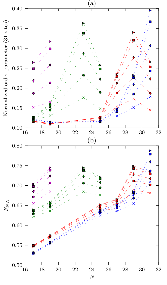
Figure 2: Degree of adiabaticity during a ramp from the superfluid to the density wave (DW) regime for a system of $N$ particles on a lattice of $L=61$ sites in the presence of a parabolic potential of strength $\alpha/U=10^{-4}$ (blue dotted lines), $10^{-3}$ (dashed red lines), $6\cdot 10^{-3}$ (dash-dotted green lines up to $N=25$), $10^{-2}$ (dash-dotted purple lines up to $N=19$). Starting from the ground state at a tunneling parameter of $J/U=0.7$, the time evolution is simulated while $J/U$ is linearly ramped down to zero within a time span $\tau\hbar/U$ with $\tau=3$ (crosses), 5 (circles), 7 (diamonds), 9 (squares), 10 (triangles). For the final state we plot (a) the normalized DW order parameter $\tilde{O}_{\mathrm{DW}}$ and (b) the nearest-neighbor fidelity $F_{\mathrm{NN}}$ with respect to the DW ground state (b). Both quantities are computed for the central region of 31 sites and approach unity in the limit of a perfectly adiabatic dynamics. The best results are found for the largest particle number $N=31$ (corresponding to “half filling”) in combination with the shallowest parabolic potential. In contrast, for the lower particle numbers $N\leq 29$ the presence of steeper potentials is always found to be favorable. As expected, the degree of adiabaticity increases with $\tau$; the tendency of the curves suggest that the results can be improved further by using ramp times larger than $\tau=10$.

We plot the main results of our simulation in Fig. 2. Both measures the DW order parameter $\tilde{O}_{\mathrm{DW}}$ and the nearest-neighbor fidelity $F_{\mathrm{NN}}$ give the same qualitative picture. We find the best result (the largest degree of adiabaticity) for the system at “half filling” with $N=31$ particles in combination with the shallowest parabolic potential. However, the degree of adiabaticity that has been achieved for generic particle numbers below half filling ($N\leq 29$) is almost as large as for half filling, and it can be increased further by tuning the potential depth $\alpha/U$ continuously to its optimal value for every particle number (instead of using only four different values of $\alpha/U$ as we do here). So we prefer not to emphasize the better results for half filling. We observe very clearly that the optimal trapping strength depends sensitively on the particle number; the optimal depth $\alpha/U$ increases when the particle number $N$ is lowered. This effect tells us that a finite parabolic inhomogeneity generally does assist the adiabatic preparation of the DW crystal. As expected, the degree of adiabaticity increases with $\tau$; the tendency of the curves suggest that the results can still be considerably improved by using ramp times larger than $\tau=10$.

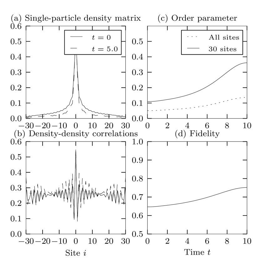
Figure 3: Sample time evolution of a system of $N=29$ particle on $L=61$ sites in the presence of the steep parabolic potential of strength $\alpha/U=10^{-3}$. The dimensionless tunneling parameter $J/U$ is linearly ramped from $0.7$ to $0$ over a duration of $\tau=10$ (in units of $\hbar/U$). (a) Single-particle density matrix $\langle\hat{b}^{\dagger}_{i}\hat{b}_{j}\rangle$ for $j=0$ at times $t=0$ (solid line) and $t=\tau/2=5$ (dashed line). (b) Density-density correlations $\braket{\hat{n}_{i}\hat{n}_{j}}$ for $j=0$ at $t=0$ and $t=\tau/2=5$. (c) Time evolution of the order parameter $\tilde{O}_{\mathrm{DW}}$ for the entire system and for a 30 site cut-out of the central part of the trap. (d) Average of the time evolution of the nearest-neighbor density matrix fidelity $F_{\mathrm{NN}}$ for the central part of the trap.

In order to get further insight, in Fig. 3 we report the time evolution of the system with $N=29$ and $\alpha/U=10^{-3}$ during the ramp with $\tau=10$. Panel (a) and (b) show the single-particle correlations $\langle\hat{b}^{{\dagger}}_{\ell}\hat{b}^{\phantom{{\dagger}}}_{0}\rangle$ and the density-density correlations $\langle\hat{n}_{\ell}\hat{n}_{0}\rangle$ both before the ramp (solid lines) and in the middle of the ramp (dashed lines). As expected, we can observe that with time the single-particle correlations (the off-diagonal order) decrease whereas the density-density correlations of the DW type are increased. This behavior is also reflected in the fact that the DW order parameter $\tilde{O}_{\mathrm{DW}}$ as well as the nearest-neighbor fidelity $F_{\mathrm{NN}}$ grow with time [panel (c) and (d)].

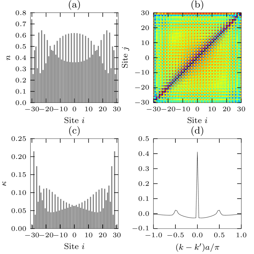
Figure 4: Final state of a system with $N=29$ particles on $L=61$ after a ramp of $J/U$ from $0.7$ to 0 with ramp duration $\tau=10$ and potential strength $\alpha/U=10^{-3}$. (a) Site occupation $\langle\hat{n}_{i}\rangle$ (b) Density-density correlations $\braket{n_{i}n_{j}}$. (c) Single-site particle number variance $\kappa_{i}=\langle\hat{n}_{i}^{2}\rangle-\langle\hat{n}_{i}\rangle^{2}$ (d) Diagonal momentum correlation function $\braket{a_{k}^{\dagger}a_{k^{\prime}}^{\dagger}a_{k^{\prime}}a_{k}}$ as it can be extracted from the shot noise correlations of time-of-flight absorption images. The satellite peaks at 0.5 are a signature of the density-wave order.

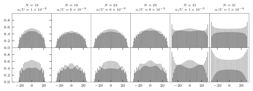
Figure 5: Density distribution before the ramp (upper row) and after the ramp (lower row) of duration $\tau\hbar/U$ with $\tau=10$ for different particle number and trap depths. The low degree of adiabaticity for $N=19$ with $\alpha/U=6\cdot 10^{-3}$ can be ascribed to the structure of the initial state. It possesses already weak DW correlations that are contaminated with kinks. The system is not able to get rid of these defects during the ramp. This behavior is found for trap depth (or particle numbers) that are smaller than optimal. The low degree of adiabaticity for both $N=25$ with $\alpha/U=6\cdot 10^{-3}$ and $31$ with $\alpha/U=1\cdot 10^{-3}$ is related to density modulations on larger scales. This behavior is found for trap depth (or particle numbers) that are larger than optimal.

A more subtle effect is visible in the density-density correlations shown in Fig. 3(b). Already for the initial state (the ground state at $J/U=0.7$, see solid line) it posseses traces of a DW-type zig-zag pattern. Superimposed to this pattern one can observe a modulation on a larger length scale (comparable to the system size) having nodes roughly at $\ell=\pm 16$. Having a closer look reveals that at these nodes the zig-zag correlations have a kink (where the maxima of the zig-zag pattern shift from even sites to odd sites or vice versa). changes from sites of even index on the one side to sites of odd index on the other side). Now, it is very difficult for the system to get rid of the kinks during the ramp as it would be required for a perfectly adiabatic evolution (since eventually at $J/U=0$ the ground state is a perfect DW). Therefore during the ramp the kinks remain, i.e. they are converted into defects. This becomes evident from Fig. 4(a) where the density distribution of the time-evolved state after the ramp is plotted (the other subfigures of Fig. 4 display more information on the final state). The presence of the kinks explains also the significant drop of the DW order parameter $\tilde{O}_{\mathrm{DW}}$ when computed not only for 31 central sites but rather for the whole system [Fig. 3(c)].

For other particle numbers and potential strengths we find similar results. Namely the initial ground state at $J/U=0.7$ possesses already a small DW-type modulation of the site occupation, typically contaminated with superimposed large scale modulations and/or a few kinks. These initial density correlations, including the kinks, are amplified when $J/U$ is lowered within a time of $\tau\hbar/U$. This behavior can be inferred from Fig. 5 that shows the initial and the final density distribution for several particle numbers and trap depths. The best (most adiabatic) results are found when there are no kinks or if the kinks lie outside the central 31-site region that we use to measure the DW order.

We find that the results are spoiled by kinks typically when the trapping potential is (according to Fig. 2) shallower than optimal for a given particle number (or the particle number is lower than optimal for a given potential strength). A typical example for kinks spoiling an adiabatic time evolution is found for $N=19$ with $\alpha/U=6\cdot 10^{-3}$ (Fig. 5). If, in turn, the trap is too steep for a given particle number (or the particle number too large for a given trap depth), we observe superimposed density modulations on larger scales in the initial state (not necessarily in combination with kinks). These modulations are still found in the time evolved state after the ramp, so they lower the degree of adiabaticity. In Fig. 5 this behavior is visible for $N=25$ with $\alpha/U=6\cdot 10^{-3}$ and $N=31$ with $\alpha/U=1\cdot 10^{-3}$.

The superimposed large-scale modulation of the DW correlations as well as the kinks that are present in the initial state and hamper an adiabatic time-evolution during the ramp cannot be explained within the simple picture of the LDA. They originate from the trap and the finite extent of the system. This suggests that the picture that in the previous section was drawn on the basis of the LDA (augmented by the assumption of smooth crossovers at phase boundaries) does not yet apply completely for the experimentally relevant system sizes of 50-100 sites only.

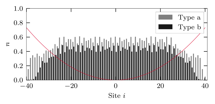
(a)

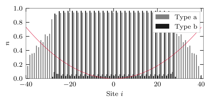
(b)

Figure 6: Site atom numbers for the two-species model in the regime used to simulate the XXZ-model with $N_{a}=39$ and $N_{b}=28$ particles. The parameters are $U_{ab}=1.0$, $\alpha_{a/b}\approx 9.1\times 10^{-4}\pm 6.0\times 10^{-7}$. The two-species system has 81 sites and effective tunneling corresponding to (a) $J/U=0.5$ ($J_{a}=J_{b}=U_{ab}/8$) and (b) $J/U=0.12$ ($J_{a}=U_{ab}/8$, $J_{b}=J_{a}/8$). The trap inhomogeneity correspond to approximately $\alpha=10^{-6}$.

One might speculate that kinks and density modulations are an artifact of the open boundary condition. However, as becomes apparent in Fig. 5, we also find kinks in the initial states for the steep trapping potentials with $\alpha/U=6\cdot 10^{-3}$ and $\alpha/U=1\cdot 10^{-2}$ for which the initial state has practically no occupation at the outermost sites such that the boundary conditions do not matter. Nevertheless, for the shallower trapping potentials, the initial state does depend on the artificial open boundary conditions and the finite size effects that we observe here can be modified when the edge of the mixed Mott insulator domain $M$ is not approximated by open boundary conditions. A more realistic model that captures also the shell surrounding the mixed Mott-insulator region $M$ is given by Eq. (3). In Fig. 6 we plot the occupation numbers of $a$ and $b$ particles for the ground state of this two-species model at $J/U=0.5$ and $J/U=0.1$ (the other parameters are specified in the caption). For the small tunneling the ground state features defect-free DW/antiferromagnetic order in the central Mott region. The small antiferromagnetic correlations found for the larger tunneling parameter are, however, contaminated with defects in a similar way as observed before when the Mott region $M$ with open boundary conditions was treated. These defects can spoil an adiabatic parameter variation towards the antiferromagnetic state plotted in Fig. 6(b).

In an experiment the DW order can be observed either in situ using high-resolution imaging techniques [61], or via time-of-flight noise correlation measurements [64, 65, 66] probing the two-particle momentum correlation function plotted in Fig. 4(d). In the latter, the signature of the DW order is given by the two satellite peaks. The fact that this feature is rather small is a consequence of the fact that in our simulations the ramp times are still not large enough. For larger ramp times (the simulation of which is numerically costly) the degree of adiabaticity is still expected to improve considerably.

6 Conclusion and outlook

We have pointed out that in a mixed Mott insulator of two bosonic atom species in an optical lattice a parabolic inhomogeneity can be created and widely tuned (between zero and large finite values) by introducing a finite potential difference for both species. And we proposed to use this control knob to investigate the role of such an inhomogeneity on the adiabatic preparation of an antiferromagnetic state (with a staggered DW pattern for each of the species). Numerical simulations of the time evolution of a model describes such a system in one dimension lead to the conclusion that a finite inhomogeneity generally assists the adiabatic preparation of the bosonic antiferromagnet. The optimal strength of the parabolic inhomogeneity depends in a sensitive way on the imbalance between the particle numbers of the two species; the larger the imbalance (i.e. the smaller the number of hard-core bosons describing the minority species) the larger the optimal strength of the inhomogeneity. We find that for a realistic system size (a mixed Mott insulator stretched over 60 sites) finite size effects that cannot be explained within the local density approximation are significant. Namely the mechanism leading to deviations from adiabaticity is related to the presence of precursing DW modulations already outside the antiferromagnetic parameter regime that – as a consequence of the finite system size – comprise imperfections like kinks. When the system is ramped into the antiferromagnetic regime these modulations, including the imperfections, are amplified.

We believe that the experimental implementation of tunable parabolic potential as we propose it here, can be a valuable tool for finding a good protocol for the preparation of antiferromagnetic order. The concept generalizes also to two and three spatial dimensions, a situation which can be addressed easily in an experiment. A theoretical study of the higher-dimensional case could be carried out on a qualitative level using Gutzwiller mean-field theory.

Another relevant question would be whether such a controllable parabolic potential can be useful also for the preparation of antiferromagnetic order in a Mott insulator of fermionic atoms [67, 68].

Appendix A Bethe-Ansatz solution of the homogeneous problem

The eigenstates of the Hamiltonian (17) with a homogeneous magnetic field $h_{\ell}\equiv h$ is found in Refs. [55, 56, 57] using the Bethe Ansatz.

Let $y$ be the total $z$-magnetization density and $\Delta=-U/2J<0$ characterizes the interaction strength. Then, $\Delta=-1$ correspond to the Heisenberg anti-ferromagnet as mentioned above.

Instead of finding the groundstate of (17) for a specific magnetic field we will instead find the ground state in each total spin-$z$ subspace, or equivalently, for fixed particle number. To find the ground state at a given magnetic field $h$, or chemical potential $\mu=h$ we should then minimize $u(\Delta,y)-\mu y$, where $u=E/L$ is the energy density of the ground state, with respect to $y$, giving $\mu=du/dy(\Delta,y)$.

In [57] the phase boundary between the SF and DW phases in Fig. 1 is given analytically by

$$-\frac{\mu}{2J}=2\sinh(\lambda)\sum_{n=-\infty}^{\infty}\frac{(-1)^{n}}{\cosh(n\lambda)},$$ (24)

where $\cosh(\lambda)=-\Delta=U/2J$.

The ground state energy density $u=E/L$ and magnetization $0<y<1$ can be found by solving the integral equations [56, Eq. (7a-c)]

$$R(\alpha) = \frac{dp}{d\alpha}-\int_{-b}^{b}K(\alpha,\beta)R(\beta)d\beta$$ (25)

$$\pi(1-y) = \int_{-b}^{b}R(\alpha)d\alpha$$ (26)

$$\frac{u(\Delta,y)}{2J} = -\frac{\Delta}{2}-\frac{2}{C}\int_{-b}^{b}R(\alpha)\frac{dp}{d\alpha}d\alpha$$ (27)

where $b\in[0,\pi]$ for $\Delta<-1$ and $b\in[0,\infty)$ for $-1<\Delta<1$ and the functions $K$ and $dp/d\alpha$ is given in [56, Table II].

For fixed $b$, the first equation is a Fredholm integral equation of the second kind, and it can be solved using the Nystrom method [69]. For fixed $b$ we can therefore solve for $R$ and, using this solution, calculate the magnetization $y$ using the second equation and the energy density $u$ using the third. The magnetic field is $\mu/U=du/dy(\Delta,y)$ which can also be found by calculating $y$ for $b\pm db$ for a small $db$ numerically and approximating the derivative using the finite difference.

One can show that the function $R$ is positive, which implies the $y$ is a one-to-one function of $b$. In order to determine the phase diagram in Fig. 1 we calculate $y$ and $\mu=de/dy$ as a function of $\Delta$ and $b$. This results in a set of (non-uniformly distributed) points $(\Delta,b,y,\mu/U)$, where we can now plot $y$ as a function of $(\Delta,\mu/U)$, or, $(J/U,\mu/U)$.

References

References

- [1] Richard P. Feynman. Simulating physics with computers. Int. J. Theor. Phys., 21:467, 1982.
- [2] Philipp Hauke, Fernando M. Cuchietti, Luca Tagliacozzo, Ivan Deutsch, and Maciej Lewenstein. Can one trust quantum simulators. Rep. Prog. Phys., 75:082401, 2012.
- [3] Immanuel Bloch, Jean Dalibard, and Sylvain Nascimbène. Quantum simulations with ultracold quantum gases. Nature Phys., 8:267, 2012.
- [4] Jacek Dziarmaga. Dynamics of a quantum phase transition and relaxation to a steady state. Adv. Phys., 59:1063, 2010.
- [5] Anatoli Polkovnikov, Krishnendu Sengupta, Alessandro Silva, and Mukund Vengalattore. Colloquium: Nonequilibrium dynamics of closed interacting quantum systems. to appear in Rev. Mod. Phys. arXiv:, 2011.
- [6] Jacek Dziarmaga, Pablo Laguna, and Wojciech H Zurek. Symmetry breaking with a slant: Topological defects after an inhomogeneous quench. Phys. Rev. Lett., 82:4749, 1999.
- [7] Jacek Dziarmaga and Marek M Rams. Dynamics of an inhomogeneous quantum phase transition. New J. Phys., 12:055007, 2010.
- [8] Jacek Dziarmaga and Marek M Rams. Adiabatic dynamics of an inhomogeneous quantum phase transition: the case of a dynamical exponent. New J. Phys., 12:103002, 2010.
- [9] Immanuel Bloch, Jean Dalibard, and Wilhelm Zwerger. Many-body physics with ultracold gases. Rev. Mod. Phys., 80:885, 2008.
- [10] Maciej Lewenstein, Anna Sanpera, and Veronica Ahufinger. Ultracold Atoms in Optical Lattices: Simulating quantum many-body systems. Oxford University Press, Oxford (UK), 2012.
- [11] Ehud Altman, Walter Hofstetter, Eugene Demler, and Mikhail D. Lukin. Phase diagram of two-component bosons on an optical lattice. N. J. Phys., 5:113, 2003.
- [12] L. M. Duan, E. Demler, and M. D. Lukin. Controlling spin exchange interactions of ultracold atoms in optical lattices. Phys. Rev. Lett., 91:090402, 2003.
- [13] A. B. Kuklov and B. V. Svistunov. Counterflow superfluidity of two-species ultracold atoms in a commensurate optical lattice. Phys. Rev. Lett., 90:100401, 2003.
- [14] A. Hubener, M. Snoek, and W. Hofstetter. Magnetic phases of two-component ultracold bosons in an optical lattice. Phys. Rev. B, 80:245109, 2009.
- [15] Stephen Powell. Magnetic phases and transitions of the two-species bose-hubbard model. Phys. Rev. A, 79:053614, 2009.
- [16] Uttam Shrestha. Antiferromagnetism in a bosonic mixture of rubidium (87rb) and potassium (41k). Phys. Rev. A, 82:041603(R), 2010.
- [17] B. Capogrosso-Sansone, S. G. Söyler, N. V. Prokof’ev, and B. Svistunov. Critical entropies for magnetic orderingin bosonic mixtures on a lattice. Phys. Rev. A, 81:053622, 2010.
- [18] Yongquiang Li, Reza Bakhtiari, Liang He, and Walter Hofstetter. Tunable anisotropic magnetism in trapped two-component bose gases. Phys. Rev. B, 84:144411, 2011.
- [19] André Eckardt, Philipp Hauke, Parvis Soltan-Panahi, Christoph Becker, Klaus Sengstock, and Maciej Lewenstein. Frustrated quantum antiferromagnetism with ultracold bosons in a triangular lattice. EPL, 89:10010, 2010.
- [20] Jonathan Simon, Waseem S. Bakr, Ruichao Ma, M. Eric Tai, Philipp M. Preiss, and Markus Greiner. Quantum simulation of antiferromagnetic spin chains in an optical lattice. Nature, 472:307, 2011.
- [21] J. Struck, C. Ölschläger, R. Le Targat, P. Soltan-Panahi, A. Eckardt, M. Lewenstein, P. Windpassinger, and K. Sengstock. Quantum simulation of frustrated classical magnetism in triangular optical lattices. Science, 333:996, 2011.
- [22] Philipp Hauke, Olivier Tieleman, Alessio Celi, Christoph Ölschläger, Juliette Simonet, Julian Struck, Malte Weinberg, Patrick Windpassinger, Klaus Sengstock, Maciej Lewenstein, and Andr Eckardt. Non-abelian gauge fields and topological insulators in shaken optical lattices. Phys. Rev. Lett., 109:145301, 2012.
- [23] Patrick A. Lee, Naoto Nagaosa, and Xiao-Gang Wen. Doping a mott insulator: Physics of high-temperature superfluidity. Rev. Mod. Phys., 78:17, 2006.
- [24] W. Hofstetter, J. I. Cirac, P. Zoller, E. Demler, and M. D. Lukin. High-temperature superfluidity of fermionic atoms in optical lattices. Phys. Rev. Lett., 89:220407, 2002.
- [25] André Eckardt and Maciej Lewenstein. Controlled hole doping of a mott insulator of ultracold fermionic atoms. Phys. Rev. A, 82:011606(R), 2010.
- [26] Jean-Sébastien Bernier, Guillaume Roux, and Corinna Kollath. Slow quench dynamics of a one-dimensional bose gas confined to an optical lattice. Phys. Rev. Lett., 106:200601, 2011.
- [27] Stefan S. Natu, Kaden R. A. Hazzard, and Erich J. Mueller. Local versus global equilibration near the bosonic mott-insulator–superfluid transition. Phys. Rev. Lett., 106:125301, 2011.
- [28] F. Hébert, G. G. Batrouni, R. T. Scalettar, G. Schmid, M. Troyer, and A. Dorneich. Quantum phase transitions in the two-dimensional hardcore boson model. Phys. Rev. B, 65:014513, 2001.
- [29] Anders S. Sørensen, Ehud Altman, Michael Gullans, J. V. Porto, Mikhail D. Lukin, and Eugene Demler. Adiabatic preparation of many-body states in optical lattices. Phys. Rev. A, 81:061603(R), 2010.
- [30] Michael Lubasch, Valentin Murg, Ulrich Schneider, J. Ignacio Cirac, and Mari-Carmen Banuls. Adiabatic preparation of a heisenberg antiferromagnet using an optical superlattice. Phys. Rev. Lett., 107:165301, 2011.
- [31] Wojciech H. Zurek. Causality in condensates: Gray solitons as relics of bec formation. Phys. Rev. Lett., 102:105702, 2009.
- [32] A. del Campo, G. De Chiara, G. Morigi, M. B. Plenio, and A. Retzker. Structural defects in ion chains by quenching the external potential: The inhomogeneous kibble-zurek mechanism. Phys. Rev. Lett., 105:075701, 2010.
- [33] A. del Campo, A Retzker, and M. B. Plenio. The inhomogeneous kibble-zurek mechanism: vortex nucleation during bose-einstein condensation. New J. Phys., 13:083022, 2011.
- [34] Masudul Haque and Frank E. Zimmer. Slow interaction ramps in trapped many-particle systems” universal deviations from adiabacity. arXiv:1110.0840, 2012.
- [35] Mario Collura and Dragi Karevski. Critical quench dynamics in confined systems. Phys. Rev. Lett., 104:200601, 2010.
- [36] Anzi Hu, Ludwig Mathey, Eite Tiesinga, Ippei Danshita, Carl J Williams, and Charles W Clark. Detecting paired and counterflow superfluidity via dipole oscillations. Phys. Rev. A, 84:041609(R), 2011.
- [37] J. Catani, L. De Sarlo, G. Barontini, F. Minardi, and M. Inguscio. Degenerate bose-bose mixture in a three-dimensional optical lattice. Phys. Rev. A, 77:1050, 2008.
- [38] Olaf Mandel, Markus Greiner, Artur Widera, Tim Rom, Theodor W. Hänsch, and Immanuel Bloch. Controlled collisions for multi-particle entanglement of optically trapped atoms. Nature, 425:937, 2003.
- [39] P. J. Lee, M. Anderlini, B. L. Brown, J̃. Sebby-Strabley, W. D. Phillips, and J.V. Porto. Sublattice addressing and spin-dependent motion of atoms in a double-well lattice. Phys. Rev. Lett., 99:020402, 2007.
- [40] David M. Weld, Patrick Medley, Hirokazu Miyake, David Hucul, David E. Pritchard, and Wolfang Ketterle. Spin gradient thermometry for ultracold atoms in optical lattices. Phys. Rev. Lett., 103:245301, 2009.
- [41] Bryce Gadway, Daniel Pertot, René Reimann, and Dominik Schneble. Superfluidity of interacting bosonic mixtures in optical lattices. Phys. Rev. Lett., 105:0031, 2010.
- [42] Patrick Medley, David M. Weld, Hirokazu Miyake, David E. Pritchard, and Wolfang Ketterle. Spin gradient demagnetization cooling of ultracold atoms. Phys. Rev. Lett., 106:195301, 2011.
- [43] P. Soltan-Panahi, J. Struck, P. Hauke, A. Bick, W. Plenkers, G. Meineke, C. Becker, P. Windpassinger, M. Lewenstein, and K. Sengstock. Multi-component quantum gases in spin-dependent hexagonal lattices. Nature Phys., 7:434, 2011.
- [44] Takeshi Fukuhara, Seiji Sugawa, Masahito Sugimoto, Shintaro Taie, and Yoshiro Takahashi. Mott insulator of ultracold alkaline-earth-metal-like atoms. Phys. Rev. A, 79:041604(R), 2009.
- [45] Seiji Sugawa, Kensuke Inaba, Shintaro Taie, Rekishu Yamazaki, Makoto Yamashita, and Yoshiro Takahashi. Interaction and filling-induced quantum phases of dual mott insulators of bosons and fermions. Nature Phys., 7:642, 2011.
- [46] Masaaki Kitagawa, Katsunari Enomoto, Kentaro Kasa, Yoshiro Takahashi, Roman Ciury, Pascal Naidon, and Paul S. Julienne. Two-color photoassociation spectroscopy of ytterbium atoms and the precise determinations of s-wave scattering lengths. Phys. Rev. A, 77:012719, 2008.
- [47] G. Thalhammer, G. Barontini, J. Catani, F. Rabatti, C. Weber, A. Simoni, F. Minardi, and M. Inguscio. Collisional and molecular spectroscopy in an ultracold bose bose mixture. New J. Phys., 11:055044, 2009.
- [48] D. J. Klein. Degenerate perturbation theory. J. Chem. Phys., 61:786, 1973.
- [49] J. Spałek and A. M. Oleś. Ferromagnetism in narrow s-band with inclusion of intersite correlations. Physica B, 86-88:375, 1977.
- [50] Z. Zou and P. W. Anderson. Neutral fermion, charge-e boson excitations in the resonating-valence-bond state and superconductivity in la2cuo4-based compounds. Phys. Rev. B, 37:627, 1988.
- [51] Massimo Boninsegni. Phase separation in mixtrues of hard core bosons. Phys. Rev. Lett., 87:087201, 2001.
- [52] Massimo Boninsegni. Phase separation and stripes in a boson version of a doped quantum antiferromagnet. Phys. Rev. B, 65:134403, 2002.
- [53] Massimo Boninsegni and Nikolay V. Profkof’ev. Phase diagram of an anisotropic bosonic - model. Phys. Rev. B, 77:092502, 2008.
- [54] M. Lewenstein, L. Santos, M. A. Baranov, and H. Fehrmann. Atomic bose-fermi mixtures in an optical lattice. Phys. Rev. Lett., 92:050401, 2004.
- [55] C. N. Yang and C. P. Yang. One-dimensional chain of anisotropic spin-spin interactions. i. proof of bethe’s hypothesis for ground state in a finite system. Phys. Rev., 150:321, 1966.
- [56] C. N. Yang and C. P. Yang. One-dimensional chain of anisotropic spin-spin interactions. ii. properties of the ground-state energy per lattice site for an infinite system. Phys. Rev., 150:327, 1966.
- [57] C. N. Yang and C. P. Yang. One-dimensional chain of anisotropic spin-spin interactions. iii. applications. Phys. Rev., 151:258, 1966.
- [58] Bill Sutherland. Beautiful Models: 70 Years of Exactly Solved Quantum Many-Body Problems. World Scientific, 2004.
- [59] F. Verstraete, V. Murg, and J. I. Cirac. Matrix product states, projected entangled pair states, and variational renormalization group methods for quantum spin systems. Adv. Phys., 57(2):143–224, 2008.
- [60] Guifre Vidal. Efficient simulation of one-dimensional quantum many-body systems. Phys. Rev. Lett., 93:040502, 2004.
- [61] W. S. Bakr, J. I. Gillen, A. Peng, S. Foelling, and M. Greiner. Quantum gas microscope detecting single atoms in a hubbard regime optical lattice. Nature, 462:74, 2009.
- [62] Jacob F Sherson, Christoph Weitenberg, Manuel Endres, Marc Cheneau, Immanuel Bloch, and Stefan Kuhr. Single-atom-resolved fluorescence imaging of an atomic mott insulator. Nature, 467:68, 2010.
- [63] Michael A Nielsen and Isaac L. Chuang. Quantum Computation and Quantum Information. Cambridge University Press, Cambridge, UK, 2000.
- [64] Ehud Altman, Eugene Demler, and Mkhail D. Lukin. Probing many-body states of ultracold atoms via noise correlations. Phys. Rev. A, 70:013603, 2004.
- [65] Radka Bach and Kazimierz Rza̧żewski. Correlations in atomic systems: Diagnosing coherent superpositions. Phys. Rev. Lett., 92:200401, 2004.
- [66] S. Fölling, F. Gerbier, A. Widera, O. Mandel, T. Gericke, and I. Bloch. Spatial quantum noise interferometry in expanding ultracold atom clouds. Nature, 434:481, 2005.
- [67] U. Schneider, L. Hackermüller, S. Will, T. Best, I. Bloch, T. A. Costi, R. W. Helmes, D. Rasch, and A. Rosch. Metallic and insulating phases of repulsively interacting fermions in a 3d optical lattice. Science, 322:1520, 2008.
- [68] Robert Jördens, Niels Strohmaier, Kenneth Günter, Henning Moritz, and Tilman Esslinger. A mott insulator of fermionic atoms in an optical lattice. Nature, 455:204, 2008.
- [69] William H. Press, Saul A. Teukolsky, William T. Vetterling, and Brian P. Flannery. Numerical Recipes 3rd Edition: The Art of Scientific Computing. Cambridge University Press, 2007.