Transport properties for liquid silicon-oxygen-iron mixtures at Earth’s core conditions

Abstract

We report on the thermal and electrical conductivities of two liquid silicon-oxygen-iron mixtures (Fe_0.82Si_0.10O_0.08 and Fe_0.79Si_0.08O_0.13), representative of the composition of the Earth’s outer core at the relevant pressure-temperature conditions, obtained from density functional theory calculations with the Kubo-Greenwood formulation. We find thermal conductivities $k$ =100 (160) W m^-1 K^-1, and electrical conductivities $\sigma=1.1(1.3)\times 10^{6}\Omega^{-1}$ m^-1 at the top (bottom) of the outer core. These new values are between 2 and 3 times higher than previous estimates, and have profound implications for our understanding of the Earth’s thermal history and the functioning of the Earth’s magnetic field, including rapid cooling rate for the whole core or high level of radiogenic elements in the core. We also show results for a number of structural and dynamic properties of the mixtures, including the partial radial distribution functions, mean square displacements, viscosities and speeds of sound.

I Introduction

Transport properties of the Earth’s core are of great importance to understand the thermal and magnetic behaviour of our planet. It is widely believed that the Earth’s core is a mixture of iron and light impurities Poirer94 . First principles calculations indicate that the liquid outer core contains a significant fraction of oxygen (between 8 or 13 %), and silicon and/or sulphur (between 8 and 10 %) alfe07 . Oxygen is expelled into the liquid upon freezing of the inner core at inner-core boundary (ICB), which helps to drive convection responsible for the generation of the Earth’s magnetic field. Vigorous convection keeps the outer core in a well-mixed state, with a temperature distribution which closely follows an adiabatic profile. Heat flows from the bottom to the top of the core by thermal conduction and by convection. High thermal conductivity reduces the heat available to drive convection (in the limit of infinite thermal conductivity the whole core would become isothermal and would not convect).

The electrical resistivity - and hence its inverse, the electrical conductivity $\sigma$ - determines the magnitude of Ohmic losses of the electric currents in the outer core that generate the magnetic field, and also the magnetic diffusion time (that is, the time that it would take for the magnetic field to decay in the absence of a generating mechanism). First experimental measurements of the electrical conductivity of pure iron combining high pressures and temperatures date back to the late sixties. They were performed on shock-compressed iron up from a few GPa to about 140 GPa and provided values for $\sigma$ in the range 1.0-1.5 $\times 10^{6}\Omega^{-1}$ m^-1 (see Ref. Keeler69 and refs. therein; also Ref. Keeler71 ). These results were in line with earlier estimates of $\sigma\simeq 1\times 10^{6}\Omega^{-1}$ m^-1 based on geophysical arguments Elsasser46 . A few decades later, Secco and Schloessin Secco89 measured the electrical conductivity of pure solid and liquid Fe at pressures up to few GPa and then extrapolated their results to high pressures and temperatures typical of the outer core. Noting the effects that the extrapolation to higher parameter values had on the function of the density of states, they derived values for $\sigma$ in the range 0.66-0.83 $\times 10^{6}\Omega^{-1}$ m^-1, which agrees well with the results previously obtained by Keeler and Mitchell Keeler69 , but is slightly smaller than the value measured by Keeler and Royce Keeler71 . More recently, the electrical conductivity of pure iron has been measured in shock compression experiments at high pressures and temperatures (up to 208 GPa and 5220 K) by Bi et al. Bi02 . Its value ranges between 0.76 and 1.45 $\times 10^{6}\Omega^{-1}$ m^-1 by reducing the pressure from about 200 to 100 GPa. These findings are in agreement with the result of about 1.0 $\times 10^{6}\Omega^{-1}$ m^-1 measured by Gomi et al. Gomi10 in analogous experiments performed with a diamond-anvil cell under high static pressure (up to 65 GPa) at room temperature. They are also close to the value $\sigma=0.8\times 10^{6}\Omega^{-1}$ m^-1 estimated by Stacey and Anderson Stacey01 , by assuming that, for a pure metal, the conductivity is constant on its melting curve. First-principles density functional theory (DFT) calculations of solid iron at low temperature and under pressure have been presented by Sha and Cohen Sha11 . Using the Bloch-Grüneisen formula they extrapolated their results up to the high pressures and temperatures studied by Bi et al., finding a slightly larger value in the range 1.1-1.8 $\times 10^{6}\Omega^{-1}$ m^-1. Recently we have calculated the electrical conductivities of pure liquid iron at the conditions of the Earth’s outer core using DFT with the Kubo-Greenwood formulation (DFT-KG), obtaining values in the range 1.4-1.6 $\times 10^{6}\Omega^{-1}$ m^-1. pozzo12 An independent calculation was also performed by de Koker et al. Koker12 showing similar values. These values agree well with the experimental findings of the older shock wave measurements of Keeler and Royce Keeler71 , but they are larger than the experimental values reported by Bi et al. above 120 GPa Bi02 .

The conductivities of the mixtures with typical core compositions were estimated by Stacey and Anderson Stacey01 to be about $0.5\times 10^{6}\Omega^{-1}$ m^-1 in the case of FeNiSi liquid alloys, by extrapolating measured resistivity values of FeSi alloys from Matassov Matassov77 experimental data. Our preliminary results of FeSiO liquid alloys at Earth’s core conditions indicated only a reduction of about $30$% of the conductivity of the mixture compared to that of pure iron pozzo12 , suggesting therefore values above $1\times 10^{6}\Omega^{-1}$ m^-1.

Estimates for the thermal conductivity $k$ for liquid iron and liquid iron mixtures ranged between 25 and 60 $m^{-1}$ K^-1. Stacey01 ; Davies07 ; Stacey07 ; Konopkova11 Our recent DFT-KG calculations for pure iron at core conditions provided values significantly higher, as expected from the relation between the thermal and the electrical conductivity as encoded in the Wiedemann-Franz law wiedemann1853 , which we found to be closely followed pozzo12 .

The DFT-KG method has been applied to a wide range of problems, including low pressure systems (C, Na, Al, Ar, Ga, Pb) Galli89 ; Holender95 ; Silvestrelli97 ; Tretiakov04 ; Recoules05 ; Knider07 , high pressure (H, H-He mixtures and Al) Morales09 ; Morales10 ; Lorenzen11 ; Vlcek12 and ultrahigh pressure (water) French10 . Here we report detailed DFT-KG calculations for $\sigma$ and $k$ of liquid iron mixtures, Fe_0.82Si_0.10O_0.08 and Fe_0.79Si_0.08O_0.13, representative of Earth’s core composition. We find $\sigma=1.1-1.3\times 10^{6}\Omega^{-1}$ m^-1 and $k=100-160$ W $m^{-1}$ K^-1, the two extremes in the ranges corresponding to the top and the bottom of the core, respectively. These values are in close agreement with extrapolations obtained from recent diamond-anvil-cell experimental measurements of the electrical resistivity by Hirose et al. Hirose11 and by Gomi et al. Gomi11 ; Gomi12 (who estimated the thermal conductivity from the resistivity using the Wiedemann-Franz law). We find the Wiedemann-Franz law to be closely followed also for the iron mixtures, although with a lower value for the Lorenz parameter.

These new values for the conductivities of the liquid outer core have profound implications for our understanding of the Earth’s thermal history and the generation of the Earth’s magnetic field.

For the typical Earth’s core mixtures investigated here we also show results for the partial radial distribution functions, mean square displacements, viscosities and the speeds of sound.

In Sec. II we describe the techniques used in the calculations. The following section contains our results, starting with the pressure-temperature profile in the core in Sec. III.1, the structural properties of the mixtures in Sec. III.2, ionic transport properties in Sec. III.3 and electronic transport properties in Sec. III.4. Sec. IV includes a discussion of the implications of our results for the Earth, and Sec. V contains the conclusions.

II Techniques

First principles simulations were performed using the vasp code kresse96 , with the projector augmented wave (PAW) method blochl94 ; kresse99 and the Perdew-Wang pw91 functional (PW91). The PAW potential for oxygen, silicon and iron have the $2s^{2}2p^{4}$, $3s^{2}3p^{2}$ and $3p^{6}4s^{1}3d^{7}$ valence electronic configurations respectively, and the core radii were 0.79, 0.8 and 1.16 Å. To calculate the electrical conductivity we also tested two additional iron PAW potentials, with $4s^{1}3d^{7}$ and $3s^{2}sp^{6}4s^{1}3d^{7}$ valence configurations and 1.16 and 0.85 Å core radii respectively. The potentials with more semi-core states included in valence only give contributions to the optical conductivity at high frequencies, but provide the same dc conductivity. For this reason, conductivities have been calculated with the PAW potential having the $4s^{1}3d^{7}$ valence electronic configuration. Single particle orbitals were expanded in plane-waves with a cutoff of 400 eV. Electronic levels were occupied according to Fermi-Dirac statistics, with an electronic temperature corresponding to the temperature of the system. An efficient extrapolation of the charge density was used to speed up the ab initio molecular dynamics simulations alfe99a , which were performed by sampling the Brillouin zone (BZ) with the $\Gamma$ point only. The temperature was controlled with a Nosé thermostat andersen80 and the time step was set to 1 fs. We ran simulations for typically 22 ps, from which we discarded the first ps to allow for equilibration.

In the adiabatic approximation the electrical conductivity of a liquid can be computed by generating a set of ionic configurations $\{R_{I}\}$ sampling the relevant pressure-temperature conditions, calculating the conductivity on each of these configurations and taking the average. For the conductivities we used the first 5 ps of the simulations to extract $N=40$ configurations $\{R_{I};I=1,N\}$ equally spaced in time. These $N$ configurations were then used to compute the electrical conductivity via the Kubo-Greenwood formula as implemented in vasp by Desjarlais Desjarlais02 . We performed simulations at several thermodynamic states spanning the conditions of the Earth’s core, details for the simulations used to compute the conductivities will be given in Sec. III.4.

The KG formula for the frequency ($\omega$) dependent optical conductivity for a system with $N_{I}$ ions at positions $R_{I}$ reads:

$$\sigma_{\bf k}(\omega;R_{I})=\frac{2\pi e^{2}\hbar^{2}}{3m^{2}\omega\Omega}\sum_{i,j=1}^{n}\sum_{\alpha=1}^{3}[F(\epsilon_{i,{\bf k}})-F(\epsilon_{j,{\bf k}})]|\langle\Psi_{j,{\bf k}}|\nabla_{\alpha}|\Psi_{i,{\bf k}}\rangle|^{2}\delta(\epsilon_{j,{\bf k}}-\epsilon_{i,{\bf k}}-\hbar\omega)$$ (1)

where $e$ and $m$ are the electron charge and mass respectively, $\hbar$ is the Plank’s constant divided by $2\pi$, $\Omega$ is the volume of the simulation cell and $n$ the number of Kohn-Sham states. The $\alpha$ sum runs over the three spatial directions, which in a liquid are all equivalent. $\Psi_{i,{\bf k}}$ is the Kohn-Sham wavefunction corresponding to eigenvalue $\epsilon_{i,{\bf k}}$, and $F(\epsilon_{i,{\bf k}})$ is the Fermi weight. The $\delta$ function is represented by a Gaussian, with a width chosen to be roughly equal to the average spacing between the eigenvalues (0.01 eV for a 157-atom system) weighted by the corresponding change in the Fermi function Desjarlais02 . Integration over the Brillouin Zone (BZ) is performed using standard methods monkhorst76 , and the frequency dependent conductivity is obtained by taking the thermal average:

$$\sigma(\omega)=\langle\sum_{\bf k}\sigma_{\bf k}(\omega;R_{I})W({\bf k})\rangle$$ (2)

where $W({\bf k})$ is the weighting factor for the point ${\bf k}$. The dc conductivity $\sigma_{0}$ is given by the value of $\sigma(\omega)$ in the limit $\omega\rightarrow 0$. The optical conductivity must obey the sum rule:

$$S=\frac{2m\Omega}{\pi e^{2}N_{e}}\int_{0}^{\infty}\sigma(\omega)d\omega=1,$$ (3)

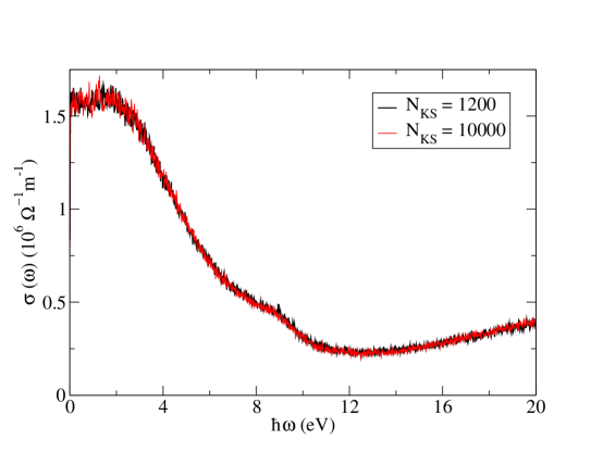
Figure 1: Optical conductivity $\sigma(\omega)$ of liquid iron as function of energy computed using N${}_{KS}=$10,000 and N${}_{KS}=$1,200 Kohn-Sham states for one configuration extracted from the ensemble at $p=328$ GPa and $T=6350$ K.

where $N_{e}$ is the number of electrons in the simulation cell. As reported earlier pozzo12b , to converge the sum rule for iron one needs to include states up to $\sim 150$ eV above the Fermi energy, which means using over 10,000 Kohn-Sham states for a typical 157 atoms simulation cell with the 8 valence electron PAW iron potential. However, only states near the Fermi energy contribute to the zero frequency limit of the optical conductivity. This is illustrated in Fig. 1, where we show $\sigma(\omega)$ as function of $\omega$ computed using both 10,000 and 1,200 Kohn-Sham states for one configuration of liquid iron extracted from the ensemble at $p=328$ GPa and $T=6350$ K. It is clear that both calculations give the same dc conductivity, so we decided to spot check the sum rule only in a limited number of cases, and then use 1,200 Kohn-Sham states for the majority of the calculations.

In a free electron liquid the electronic part of the thermal conductivity $\kappa_{0}$ and the electrical conductivity $\sigma_{0}$ are related by the Wiedemann-Franz law, $L=\kappa_{0}/\sigma_{0}T$, where $L$ is the Lorenz number. In a real liquid the validity of the Wiedemann-Franz law is not necessarily expected, and in fact a number of exceptions for metals at near ambient conditions are known (see e.g. Kittel kittel ). Here we have directly calculated $\kappa_{0}$ using the Chester-Thellung chester61 (CS) formulation of the Kubo-Greenwood formula, which reads:

$$\kappa(\omega)=\frac{1}{e^{2}T}\left(L_{22}(\omega)-\frac{L_{12}(\omega)^{2}}{\sigma(\omega)}\right),$$ (4)

and $\kappa_{0}$ is the value of $\kappa(\omega)$ in the limit $\omega\rightarrow 0$. The kinetic coefficients $L_{lm}(\omega)$ are given by mazevet10 :

$$L_{lm}(\omega)=(-1)^{(l+m)}\frac{2\pi e^{2}\hbar^{2}}{3m^{2}\omega\Omega}\sum_{i,j=1}^{n}\sum_{\alpha=1}^{3}[F(\epsilon_{i,{\bf k}})-F(\epsilon_{j,{\bf k}})]|\langle\Psi_{j,{\bf k}}|\nabla_{\alpha}|\Psi_{i,{\bf k}}\rangle|^{2}\times$$ (5)

$$\times\left[\epsilon_{j,{\bf k}}-\mu\right]^{(l-1)}\left[\epsilon_{i,{\bf k}}-\mu\right]^{(m-1)}\delta(\epsilon_{j,{\bf k}}-\epsilon_{i,{\bf k}}-\hbar\omega),$$

where $\mu$ is the chemical potential. The implementation of the CS formula in vasp is also due to Desjarlais Desjarlais02 .

We checked convergence of the conductivities with respect to the size of the system by performing calculations with cubic simulation cells including 67, 157 and 288 atoms and using up to 6 k-points to sample the BZ. We found that even the smallest cell sampled with the single k-point (1/4,1/4,1/4) gives results converged to better than 1%. We then decided to use 157-atom simulation cells.

III Results

III.1 Pressure-temperature profile

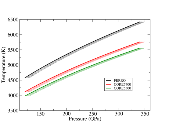
Figure 2: Adiabatic temperature profiles as function of pressure anchored by three possible ICB temperatures $T_{\rm ICB}$. Black curve (FERRO) corresponds to $T_{\rm ICB}=6350$ K. Red curve (CORE5700) to $T_{\rm ICB}=5700$ K, and green curve to $T_{\rm ICB}=5500$ K. Low pressure edges of the bands (solid line) correspond to the raw DFT-PW91 pressures, high pressure edges to pressure corrected by 10 GPa, which is the typical DFT-PW91 underestimate of the pressure for iron at core conditions (see text for details).

The Earth’s outer core is convecting, and therefore it is assumed to be in a well mixed state with an adiabatic pressure-temperature ($p,T$) profile. This can be determined by fixing the temperature $T$ at the ICB pressure $p=329$ GPa and following the line of constant entropy up to the CMB pressure $p=136$  GPa. In Fig. 2 we show the $p,T$ profiles that we used in the present work, obtained by fixing three possible ICB temperatures: the melting temperature of pure iron T = 6350 K alfe02 ; alfe09 (FERRO), the melting temperature of the mixture Fe_0.82Si_0.10O_0.08 T = 5700 K (CORE5700) alfe02b , and the melting temperature of the mixture Fe_0.79Si_0.08O_0.13 (CORE5500) alfe07 . The mixtures are two possible estimates for the composition of the Earth’s outer core, which match the Preliminary Reference Earth Model (PREM) ICB density jump of 4.5% dziewonski81 , and the more recent ICB density jump of 6.3% proposed by Masters and Gubbins masters03 , respectively. The adiabats are shown as bands, with the low pressure (solid) edge corresponding to the actual DFT-PW91 values, and the high pressure edge to pressures increased by 10 GPa, which is the approximate amount by which DFT-PW91 underestimates the pressure of solid iron at Earth’s core conditions alfe02 .

III.2 Structure

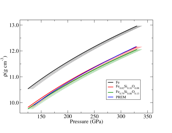
Figure 3: Density profiles for pure iron (black), the Fe_0.82Si_0.10O_0.08 mixture (red), and the Fe_0.79Si_0.08O_0.13 mixture (green) on the respective FERRO, CORE5700 and CORE5500 pressure-temperature profiles displayed in Fig. 2. Bands have the same meaning as in Fig. 2. PREM density profile dziewonski81 is shown with blue line.

In Fig. 3 we show the densities $\rho$ of the three possible cases mentioned in Sec. III.1 on the respective adiabats. They are shown as bands also in this case, with the same meaning as in Fig. 2. The raw DFT-PW91 density of the Fe_0.82Si_0.10O_0.08 (approximated by a simulation cell containing 129 iron atoms, 16 silicon atoms and 12 oxygen atoms) mixture matches the PREM density of the liquid side of the ICB by construction alfe02b , while the mixture Fe_0.79Si_0.08O_0.13 (125 irons, 12 silicons and 20 oxygens) has a slightly lower ICB density but appears to match quite well the CMB density.

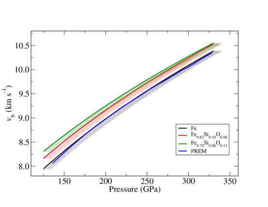
Figure 4: Bulk sound velocity for pure iron (black), the Fe_0.82Si_0.10O_0.08 mixture (red), and the Fe_0.79Si_0.08O_0.13 mixture (green) on the respective FERRO, CORE5700 and CORE5500 pressure-temperature profiles displayed in Fig. 2. Bands have the same meaning as in Fig. 2. The PREM bulk sound velocities dziewonski81 are shown in blue.

In Fig. 4 we plot the bulk sound velocities as function of pressure for pure iron and for the two mixtures, compared with PREM. These are defined as $v_{b}=\sqrt{(K_{S}/\rho)}$, where $K_{S}=-V(dp/dV)_{S}$ is the isentropic bulk modulus, with $V$ and $S$ the volume and the entropy of the system, respectively. To compute $K_{S}$ we fitted the pressures computed along the adiabats to a Murnaghan equation of state murnaghan :

$$p(V)=\frac{K_{0}}{K^{\prime}_{0}}\left[\left(\frac{V_{0}}{V}\right)^{K^{\prime}_{0}}-1\right]$$ (6)

where $K_{0}$ is the zero pressure bulk modulus and $K^{\prime}_{0}=(dK/dp)_{p=0}$. Interestingly, the bulk sound velocities of pure DFT-PW91 iron are very close to PREM, although the agreement is worsened when the pressure correction of 10 GPa is applied to the DFT-PW91 calculations. By contrast, the pressure corrected values for the Fe_0.82Si_0.10O_0.08 mixture sit very close to PREM. As expected, the combination of lower temperatures and densities has the effect of increasing the bulk sound velocities.

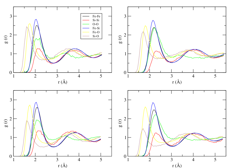
Figure 5: Partial radial distribution functions for the mixture Fe_0.82Si_0.10O_0.08 close to ICB (a) and CMB (b) conditions, and those for the mixture Fe_0.79Si_0.08O_0.13 close to ICB (c) and CMB (d) conditions (see text for details).

In Fig. 5 we show the partial radial distribution functions (rdf) $g_{FeFe}(r)$, $g_{SiSi}(r)$, $g_{OO}(r)$, $g_{FeSi}(r)$, $g_{FeO}(r)$ and $g_{SiO}(r)$. They are defined so that, by sitting on an atom of the species $\alpha$, the probability of finding an atom of the species $\beta$ in the spherical shell $(r,r+dr)$ is $4\pi r^{2}n_{\beta}g_{\alpha\beta}(r)dr$, where $n_{\beta}$ is the number density of the species $\beta$. Fig. 5 (a) shows the partial rdfs for the mixture Fe_0.82Si_0.10O_0.08 at $(p,T)=(329~{}{\rm GPa},5700~{}{\rm K})$. In agreement with our previous simulations on FeO mixtures alfe99 , the present partial rdfs show that the distance between neighbouring iron and oxygen atoms (obtained from the position of the first peak of $g_{FeO}(r)$ at $\sim 1.7$ Å) is significantly shorter than the iron-iron distance ($\sim 2.1$ Å) or the oxygen-oxygen distance ($\sim 2.1$ Å) . This indicates that oxygen atoms have two effective radii, one for the interaction with themselves, and a different one for the interaction with an iron atom. The relatively large oxygen-oxygen distance suggests than oxygen atoms effectively repel each other at the typical single and double bond oxygen distances (1.47 Å  and 1.21 Å, respectively) alfe99 . The situation is rather different for the silicon-silicon and the iron-silicon distances, as the first peaks of $g_{SiSi}(r)$ and $g_{FeSi}(r)$ are roughly in the same place, showing that iron and silicon atoms have one single effective radius when interacting with each other or with themselves, and also that this effective radius is similar for the two atoms. For the silicon-oxygen interaction, the position of the first peak of $g_{SiO}(r)$ at $\sim 1.6$ Å is at slightly shorter distance than that of $g_{FeO}(r)$, indicating that the silicon-oxygen bond is shorter and probably stronger when compared to the iron-oxygen bond. Although it could be suggested that oxygen and silicon in liquid iron may precipitate out as SiO₂, the simulations provided no evidence of any phase separation or departure from a well mixed liquid. In Fig. 5 (b) we show the partial rdfs for the same mixture at $(p,T)=(134~{}{\rm GPa},4260~{}{\rm K})$ (close to CMB conditions), and in Fig. 5 (c,d) those for the mixture Fe_0.79Si_0.08O_0.13 at $(p,T)=(328~{}{\rm GPa},5500~{}{\rm K})$ and $(p,T)=(134~{}{\rm GPa},4112~{}{\rm K}$), respectively. There are no significant differences between the corresponding partial rdfs for the two mixtures, and the only effect of moving from CMB to ICB conditions is that of decreasing the height of the $g_{OO}(r)$ peak and increasing the height of the $g_{SiO}(r)$ peak, which implies that the oxygen-silicon coordination number is slightly increased with pressure. No noticeable pressure effect is observed for the iron-oxygen interactions.

III.3 Ionic transport

In this section we describe the ionic dynamical properties of the system, including atomic self-diffusion coefficients and viscosities. The self-diffusion coefficient $D$ can be obtained from the asymptotic slope of the time dependent mean square displacement (MSD) $M(t)$ in the long time limit $t\rightarrow\infty$:

$$M(t)=\frac{1}{N_{I}}\sum_{i=1}^{N_{I}}\langle|{\bf r_{i}}(t+t_{0})-{\bf r_{i}}(t_{0})|^{2}\rangle$$

$$D=\frac{1}{6}\lim_{t\rightarrow\infty}\frac{dM(t)}{dt}$$

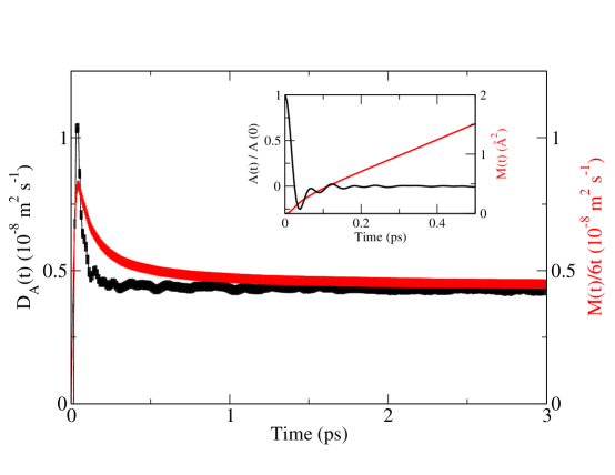
Figure 6: Self-diffusion coefficient as a function of time obtained from the time dependent mean square displacement $M(t)$ (red) and the velocity-velocity autocorrelation function $D_{A}(t)$(black) (see text details). Also shown in the inset the value of $M(t)$ and $A(t)/A(0)$ as a function of time. Results correspond to the iron atoms in the Fe_0.82Si_0.10O_0.08 mixture at ICB conditions.

where $\langle\cdot\rangle$ has the meaning of thermal average, which is computed as time average over different origins $t_{0}$ along the molecular dynamics simulation, ${\bf r_{i}}(t)$ is the vector position at time t of the i-th atom, and $N_{I}$ is the number of ions. In the inset of Fig. 6 we show the value of $M(t)$ as function of time for the iron atoms in the Fe_0.82Si_0.10O_0.08 mixture at ICB conditions. It is clear that after a transient of $\sim 0.2$ ps the linear behaviour of $M(t)$ is well established. The initial part of the transient is due to atoms moving freely before collisions begin to occur, and for this reason the MSD increases as the square of time.

An alternative route to the self-diffusion coefficient is through the Green-Kubo (GK) relations, which relate transport coefficients and correlation functions allen . The self-diffusion coefficient $D$ is given by the integral of the velocity-velocity autocorrelation function (VACF) $A(t)$:

$$A(t)=\langle{\bf v}_{i}(t+t_{0})\cdot{\bf v}_{i}(t_{0})\rangle$$

$$D_{A}(t)=\frac{1}{3}\int_{0}^{t}d\tau A(\tau)$$

$$D=\lim_{t\rightarrow\infty}D_{A}(t)$$

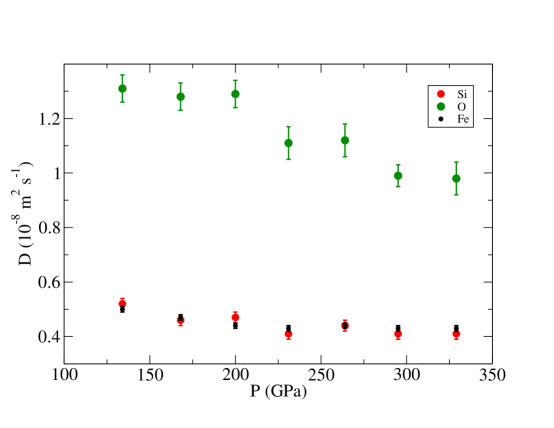
Figure 7: Self diffusion coefficients of Fe, Si and O atoms vs pressure for the Fe_0.82Si_0.10O_0.08 mixture. Temperatures are determined from the CORE5700 adiabat at the corresponding pressures.

The function $A(t)/A(0)$ is also plotted in the inset of Fig. 6, where it can be seen that correlations quickly decay to zero as soon as the atoms begin to collide with each other. In the main part of Fig. 6 we show the value of $M(t)$ divided by $6t$, and that of $D_{A}(t)$ as function of time, together with their statistical errors computed by analysing the scattering of the MSD and VACF of each atom. The two methods provide the same value for $D$ in the limit of large $t$, with $D_{A}(t)$ converging faster. In Fig. 7 and  8 we show the values of the self diffusion coefficients of iron, silicon and oxygen for the two mixtures. The values are almost constant along the adiabats, with diffusion slowing down only marginally with pressure. Interestingly, iron and silicon have very similar diffusion coefficients, despite a factor of two difference in their masses, while oxygen has a diffusion coefficient which is more than two times bigger. No significant differences are observed for the two different mixtures.

To compute the viscosities of the mixtures we used the Green-Kubo relation, which relates the shear viscosity $\eta$ to the integral of the autocorrelation function of the off-diagonal components of the stress tensor (SACF) $C_{\alpha\beta}(t)=\langle P_{\alpha\beta}(t+t_{0})P_{\alpha\beta}(t_{0})\rangle$, where $P_{\alpha\beta}$ is an off-diagonal component of the stress tensor, with $\alpha$ and $\beta$ indicating Cartesian components. There are five independent components of the traceless stress tensor: $P_{xy}$, $P_{yz}$, $P_{zx}$, $\frac{1}{2}(P_{xx}-P_{yy})$ and $\frac{1}{2}(P_{yy}-P_{zz})$ alfe98 . In a liquid these five components are equivalent, and they can all be used to improve the statistical accuracy of the viscosity integral. The shear viscosity $\eta$ is then obtained from:

$$\eta(t)=\frac{V}{k_{B}T}\int_{0}^{t}d\tau S(\tau)$$

$$\eta=\lim_{t\rightarrow\infty}\eta(t)$$

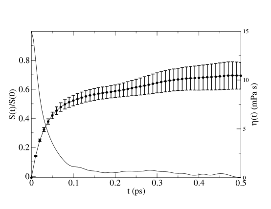
Figure 9: Average over the five independent components of the autocorrelation function of the traceless stress tensor $S(t)$, normalised by dividing by $S(0)$. Also shown is the viscosity integral $\eta(t)$ with its statistical error. Results correspond to the Fe_0.82Si_0.10O_0.08 mixture at ICB conditions (see text for details).

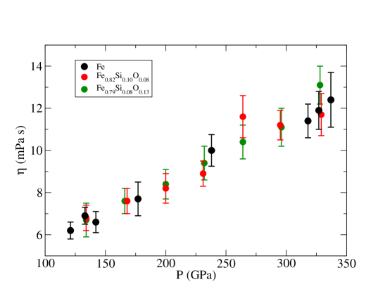
Figure 10: Viscosity as a function of pressure for the pure iron on the FERRO adiabat, and for the mixtures Fe_0.82Si_0.10O_0.08 and Fe_0.79Si_0.08O_0.13 on the CORE5700 and CORE5500 adiabats, respectively.

where $k_{B}$ is the Boltzmann constant and $S(t)=\frac{1}{5}[C_{xy}(t)+C_{yz}(t)+C_{zx}+\frac{1}{2}(C_{xx}(t)-C_{yy}(t))+\frac{1}{2}(C_{yy}(t)-C_{zz}(t))]$. In Fig. 9 we plot $S(t)/S(0)$ and $\eta(t)$ for the Fe_0.82Si_0.10O_0.08 mixture at ICB conditions. To obtain the shear viscosity $\eta$ we need to integrate $S(t)$ to $t=\infty$, however, it is clear that the $S(t)$ has decayed to zero after $\sim 0.2$ ps, after which one only integrates statistical noise. For this reason, we decided to stop the integration at $t=0.2$ ps. The viscosity integral $\eta(t)$ is also plotted in Fig. 9, together with its error bar estimated by the scattering of the five independent components of the traceless SACF. To improve the statistics on the estimate of the statistical error on $\eta(t)$ we split the simulations in two independent chunks. The viscosities are plotted in Fig. 10 for the two mixtures on the corresponding CORE5700 and CORE5500 adiabats. Their values range between $\sim 7$ mPa s at the CMB and $\sim 12$ mPa s at the ICB, with little difference between the viscosities of the two mixtures. We also report the viscosities of pure iron on the FERRO adiabat, which are consistent with those reported before dewijs98 ; alfe00 , and they have roughly the same values as those of the mixtures.

To conclude this section we also report the ionic component of the thermal conductivity of pure iron, $\kappa_{ion}$, computed using a simple pair potential, which describes the energetics and the structural and dynamical properties of iron very accurately alfe00 . The pair potential has the form $U({\bf r}_{1},\dots,{\bf r}_{N_{I}})=4\sum_{i=1,i<j}^{N_{I}}(\sigma/|{\bf r}_{i}-{\bf r}_{j}|)^{\alpha}$, where $\{{\bf r}_{i}\}$ are the Cartesian coordinates of the atoms, $\alpha=5.86$, and $\sigma=1.77$ Å. The Kubo-Green formula for the ionic thermal conductivity reads:

$$\kappa_{ion}=\frac{1}{3\Omega k_{B}T^{2}}\int_{0}^{\infty}dt\langle{\bf j}(t+t_{0})\cdot{\bf j}(t_{0})\rangle$$ (10)

where the microscopic heat current is given by:

$${\bf j}(t)=\sum_{i=1}^{N_{I}}{\bf v}_{i}\epsilon_{i}+\frac{1}{2}\sum_{i,j=1;j\neq j}^{N_{I}}{\bf r}_{ij}({\bf F}_{ij}\cdot{\bf v}_{i})$$ (11)

with ${\bf v}_{i}$ the velocity of atom $i$, ${\bf r}_{ij}$ the vector distance between atom $i$ and atom $j$, and ${\bf F}_{ij}$ the force on atom $i$ due to atom $j$ from the pair potential. The on-site energy $\epsilon_{i}$ is:

$$\epsilon_{i}=\frac{1}{2}m|{\bf v}_{i}|^{2}+\frac{1}{2}\sum_{j=1}^{N_{I}}4\left(\frac{\sigma}{|{\bf r}_{i}-{\bf r}_{j}|}\right)^{\alpha}$$ (12)

with $m$ being the mass of the atoms. The calculated values range between 2.5 and 4 W m^-1 K^-1, which compared to the electronic contribution to the thermal conductivity (see next section) are completely negligible.

III.4 Electronic transport

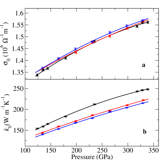
Figure 11: Electrical (a) and thermal (b) conductivity of liquid iron at Earth’s core conditions, computed on the FERRO (black), CORE5700 (red) and CORE5500 (blue) adiabats. Lines are quadratic fits to the first principle raw data (symbols). Error bars (2 s.d.) are estimated from the scattering of the data obtained from 40 statistical independent configurations. Results are obtained with cells including 157 atoms and the single k-point (1/4,1/4,1/4), which are sufficient to obtain convergence within less than 1%.

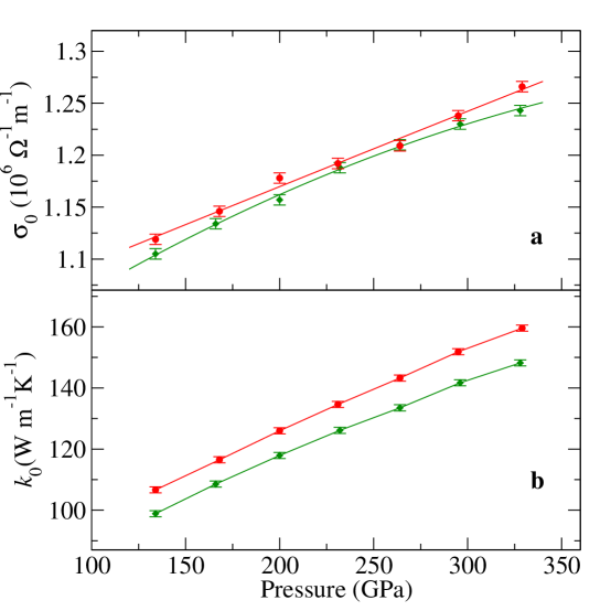
Figure 12: Electrical (a) and thermal (b) conductivity of liquid Fe_0.82Si_0.10O_0.08 (red) and liquid Fe_0.79Si_0.08O_0.13 (green) mixtures on the CORE5700 and CORE5500 adiabats, respectively. Error bars (2 s.d.) are estimated from the scattering of the data obtained from 40 statistical independent configurations. Results are obtained with cells including 157 atoms and the single k-point (1/4,1/4,1/4), which are sufficient to obtain convergence within less than 1%.

The electrical and thermal conductivity of pure iron on the three adiabats shown in Fig. 11 have been reported before pozzo12 , where we also mentioned that preliminary results showed that light impurities have the effect of reducing the conductivities of pure iron by $\sim 30\%$. Here in Fig. 12 we report the full calculations on the CORE5500 and the CORE5700 adiabats for the mixtures. It is clear that indeed the effect of the light impurities is that of reducing the conductivities of pure iron by the reported amount of $\sim 30\%$, and that the slightly different composition of the two mixtures has roughly the same reduction effect. The values for the electrical and thermal conductivities are in the range 1.1-1.3 $\times 10^{6}\Omega^{-1}$ m^-1 and 100-160 W m^-1 K^-1, respectively, with the low/high values corresponding to CMB/ICB pressure-temperature conditions.

The Lorenz parameter is roughly constant on all three adiabats, indicating that the Wiedemann-Franz law is valid throughout the core. For pure iron, the Lorenz parameter varies between 2.47 $\times 10^{-8}$ W $\Omega$ K^-2 and 2.51 $\times 10^{-}8$ W $\Omega$ K^-2, only slightly higher than its ideal value of 2.44 $\times 10^{-8}$ W $\Omega$ K^-2, while for the mixtures it is reduced in the range 2.17-2.24 $\times 10^{-8}$ W $\Omega$ K^-2.

The values we find for the conductivities and the Lorenz number are in broad agreement with those recently reported by de Koker et al. Koker12 . Our electrical conductivities are also in fairly good agreement with the experimental data for FeSi up to 140 GPa of Matassov Matassov77 and for Fe_0.94O up to 155 GPa of Knittle et al. Knittle86 , who reported values in the range 1.0-1.2 $\times 10^{6}\Omega^{-1}$ m^-1. Our thermal conductivities are also in agreement with recent experimental findings of Hirose et al. Hirose11 who reported values for the top of the outer core in the range 90-130 W m^-1 K^-1.

All results are summarised in Table I, II and III.

IV Implications for the Earth

The estimates of thermal and electrical conductivity in Tables 2 and 3 are $2-3$ times higher than those currently used in the geophysical literature (e.g. Stacey07a, ; Nimmo07, ). The high thermal conductivity in particular has significant implications for the evolution of the core and the dynamo process generating the Earth’s magnetic field. The convective motions in the outer core that are responsible for the Earth’s dynamo are driven by a combination of thermal and chemical buoyancy sources. The strength of thermal driving is measured by the amount of excess heat that cannot be conducted down the adiabatic gradient; higher thermal conductivity increases adiabatic conduction and therefore decreases the effectiveness of thermal buoyancy relative to chemical buoyancy. Maintaining the same magnetic field with less available thermal buoyancy requires a faster core cooling rate or a higher concentration of radiogenic elements in the core or a combination of the two. Moreover, a faster cooling rate implies that the inner core, which is already thought to be a relatively young feature of the Earth (age $\sim$ 1Ga, Labrosse01 ), is even younger.

The reduction in thermal buoyancy due to increased adiabatic conduction is so great that parts of the liquid core are very likely to be subcritical to thermal convection. Chemical convection, driven by release of light elements at the boundary of the solid inner core on freezing, may still be able to stir these regions, heat being transported downwards to maintain the adiabatic gradient Loper78 . Near the top of the core chemical convection weakens because of the barrier of the core-mantle boundary (CMB); here the liquid is likely to be density stratified with little or no vertical motion at all pozzo12 . Such a stable layer could be detected observationally, either by seismology or by its effect on the geomagnetic field.

It has been suggested that the heat convected away from the inner core may vary so much from place to place that the surface may be melting in some places, freezing in others, with a net growth from freezing over the whole surface Gubbins11 . The increase in thermal conductivity with depth (Tables 2 and 3) increases the heat conducted away from the ICB, making the chance of melting rather less likely. It also reduces the vigour of thermal convection deep in the core.

The main consequence of a higher electrical conductivity is to lengthen the ohmic diffusion time, the main time scale used when interpreting geomagnetic and paleomagnetic phenomena. Doubling or trebling the time scale affects virtually all interpretations to a certain extent: the dipole decay time increases from $25$ kyr to $75$ kyr. For example, it improves the ”frozen-flux” assumption, commonly used to interpret recent geomagnetic secular variation Holme07 , changes on time scales of decades-to-centuries; a polarity reversal that can take anything from 1 to 10 kyr now appears fast on the diffusion time scale. The magnetic Reynolds number for the dynamo is also larger, making dynamo action possible with lower flow speeds. Lastly, the inner core has been thought to provide a stabilising influence because its ohmic diffusion time (5,000 years) is longer than the advective time in the outer core (500 years) Gubbins99 . The higher electrical conductivity reported in this paper increases the diffusion time considerably, making the stabilising effect even stronger.

The ab-initio results also have implications for numerical models of the geodynamo. The equations governing the geodynamo process are usually cast into nondimensional form; it is well known that fundamental aspects of the solutions depend critically on the values of the dimensionless parameters. Common dimensionless parameters are the thermal Prandtl number $Pr_{T}=\nu/D_{T}$, the ratio of viscous and thermal diffusion, the magnetic Prandtl number $Pm=\nu/D_{B}$, the ratio of viscous and magnetic diffusion, and the chemical Prandtl number $Pr_{\rm X}=\nu/D_{\rm X}$, the ratio of viscous diffusion and mass diffusion for species $\rm{X}=$O,Si. Here $\nu=\eta/\rho$ is the kinematic viscosity, $D_{T}=\kappa_{0}/\rho C_{p}$ is the thermal diffusivity where $C_{p}$ is the specific heat at constant pressure, and $D_{B}=1/(\mu_{0}\sigma_{0})$ is the magnetic diffusivity where $\mu_{0}$ is the permeability of free space.

In Table 4 we list values for the Prandtl numbers using the results of our ab initio calculations (Tables 2 and 3) at the CMB (P=134 GPa) and ICB together with errors. $Pm$ is slightly higher than a previous estimate of $6\times 10^{-7}$ Gubbins , but this is still too low to be achievable in a simulation in the near future. Values of $Pr_{T}$ are lower than the value $Pr_{T}=0.1$ commonly assumed for liquid metals and can certainly be accommodated in current geodynamo models. The values of $Pr_{\rm Si}$ and $Pr_{\rm O}$ differ significantly and are larger than previous estimates Gubbins . The Lewis number $Le=Pr_{\rm O}/Pr_{T}$, an important parameter in dynamo models driven by both thermal and compositional buoyancy, is found to be $O(10^{3})$.

V Conclusions

In this work we have studied the transport properties for two liquid silicon-oxygen-iron mixtures, i.e., Fe_0.79Si_0.08O_0.13 and Fe_0.82Si_0.10O_0.08, at Earth’s core conditions using DFT-KG ab-initio theoretical calculations. We find that both the thermal and electrical conductivity of the mixtures are higher than previous estimates, the former being in the range of 100-160 W $m^{-1}$ K^-1 and the latter in the range of 1.1-1.3 $\times 10^{6}\Omega^{-1}$ m^-1. The validity of the Wiedemann-Franz law is found to be satisfied quite accurately for both iron mixtures at core conditions, the Lorenz parameter being roughly constant within the range 2.17-2.24 $\times 10^{-}8$ W $\Omega$ K^-2, only slightly higher than the ideal value of 2.44 $\times 10^{-}8$ W $\Omega$ K^-2. The values we find for the conductivities are 2 to 3 times higher than those which have been used until now and have profound implications for our understanding of the outer core evolution and the geodynamo. In particular, the inner core is now younger than previously thought, the top of the core is very likely to be thermally stably stratified, while the possibility that the inner core is partially melting is less likely. Finally, we list values for the dimensionless input parameters used in geodynamo simulations, calculated directly from the ab initio calculations.

P	T	$\rho$	$v_{b}$	$D_{Fe}$			$\eta$	$\sigma_{0}$	$\kappa_{0}$	L
GPa	K	g cm-3	km s-1	10-8m2s-1			mPa s	$10^{6}\Omega^{-1}$ m-1	W m-1 K-1	$10^{-8}$ W $\Omega$ K-2
339	6420	13.16	10.48	0.50(1)			12.4(13)	1.561(5)	248(1)	2.47(2)
328	6350	12.95	10.36	0.50(1)			11.9(9)	1.560(5)	246(1)	2.48(2)
318	6282	12.86	10.27	0.53(1)			11.4(8)	1.544(5)	243(1)	2.50(2)
240	5700	12.05	9.45	0.55(1)			10.0(8)	1.480(5)	212(1)	2.51(2)
178	5200	11.30	8.70	0.57(1)			7.7(8)	1.410(5)	183(1)	2.50(2)
144	4837	10.83	8.23	0.60(1)			6.6(5)	1.366(5)	165(1)	2.50(2)
135	4700	10.69	8.10	0.58(1)			6.9(4)	1.360(5)	159(1)	2.49(2)
124	4630	10.52	7.93	0.59(1)			6.2(4)	1.338(5)	154(1)	2.49(2)

Table 1: Pressure (P), temperature (T), density ($\rho$), bulk sound velocities ($v_{b}$), iron diffusion coefficient ($D_{Fe}$), viscosity ($\eta$), electrical conductivity ($\sigma_{0}$), thermal conductivity ($\kappa_{0}$) and Lorenz parameter (L) for pure liquid iron on the FERRO adiabat.

P	T	$\rho$	$v_{b}$	$D_{Fe}$	$D_{Si}$	$D_{O}$	$\eta$	$\sigma_{0}$	$\kappa_{0}$	L
GPa	K	g cm-3	km s-1	10-8m2s-1	10-8m2s-1	10-8m2s-1	mPa s	$10^{6}\Omega^{-1}$ m-1	W m-1 K-1	$10^{-8}$ W $\Omega$ K-2
329	5700	12.16	10.52	0.43(1)	0.41(2)	0.98(6)	11.7(10)	1.266(5)	160(1)	2.21(2)
295	5490	11.83	10.19	0.43(1)	0.41(2)	0.99(4)	11.2(7)	1.238(5)	152(1)	2.23(2)
264	5280	11.53	9.88	0.44(1)	0.44(2)	1.12(6)	11.6(10)	1.209(5)	143(1)	2.24(2)
231	5050	11.18	9.52	0.43(1)	0.41(2)	1.11(6)	8.9(6)	1.192(5)	135(1)	2.24(2)
200	4810	10.82	9.16	0.44(1)	0.47(2)	1.29(5)	8.2(7)	1.178(5)	126(1)	2.22(2)
168	4550	10.42	8.76	0.47(1)	0.46(2)	1.28(5)	7.6(6)	1.146(5)	117(1)	2.23(2)
134	4260	9.958	8.29	0.50(1)	0.52(2)	1.31(5)	6.8(6)	1.119(5)	107(1)	2.24(2)

Table 2: Pressure (P), temperature (T), density ($\rho$), bulk sound velocities ($v_{b}$), diffusion coefficients for iron ($D_{Fe}$), silicon ($D_{Si}$) and oxygen ($D_{O}$), viscosity ($\eta$), electrical conductivity ($\sigma_{0}$), thermal conductivity ($\kappa_{0}$) and Lorenz parameter (L) for the Fe_0.82Si_0.10O_0.08 liquid mixture on the CORE5700 adiabat.

P	T	$\rho$	$v_{b}$	$D_{Fe}$	$D_{Si}$	$D_{O}$	$\eta$	$\sigma_{0}$	$\kappa_{0}$	L
GPa	K	g cm-3	km s-1	10-8m2s-1	10-8m2s-1	10-8m2s-1	mPa s	$10^{6}\Omega^{-1}$ m-1	W m-1 K-1	$10^{-8}$ W $\Omega$ K-2
328	5500	12.04	10.53	0.38(1)	0.38(1)	0.92(3)	13.1(9)	1.243(5)	148(1)	2.17(2)
296	5300	11.75	10.24	0.37(1)	0.38(2)	0.90(4)	11.4(9)	1.230(5)	142(1)	2.17(2)
264	5095	11.42	9.93	0.38(1)	0.38(2)	0.98(3)	10.4(8)	1.210(5)	134(1)	2.17(2)
232	4870	11.10	9.60	0.41(1)	0.41(3)	1.00(3)	9.4(8)	1.188(5)	126(1)	2.18(2)
200	4640	10.73	9.25	0.41(1)	0.40(3)	1.19(3)	8.4(7)	1.157(5)	118(1)	2.20(2)
166	4385	10.32	8.84	0.46(1)	0.45(2)	1.19(4)	7.6(6)	1.134(5)	109(1)	2.18(2)
134	4112	9.887	8.43	0.45(1)	0.46(2)	1.30(7)	6.7(8)	1.105(5)	99(1)	2.18(2)

Table 3: Pressure (P), temperature (T), density ($\rho$), bulk sound velocities ($v_{b}$), diffusion coefficients for iron ($D_{Fe}$), silicon ($D_{Si}$) and oxygen ($D_{O}$), viscosity ($\eta$), electrical conductivity ($\sigma_{0}$), thermal conductivity ($\kappa_{0}$) and Lorenz parameter (L) for the Fe_0.79Si_0.08O_0.13 liquid mixture on the CORE5500 adiabat.

P	$Pr_{T}$	$Pm$ $\times 10^{-6}$	$Pr_{\rm Si}$	$Pr_{\rm O}$	$D_{T}$ $\times 10^{-5}$
328	0.063 (0.004)	1.7 (0.12)	286 (27)	118 (12)	1.7 (0.03)
134	0.048 (0.005)	0.9 (0.11)	147 (24)	52 (9)	1.4 (0.02)
329	0.052 (0.004)	1.5 (0.13)	235 (31)	98 (14)	1.8 (0.03)
134	0.046 (0.005)	1.0 (0.09)	131 (16)	52 (7)	1.5 (0.02)

Table 4: Values of the thermal Prandtl number ($Pr_{T}$), magnetic Prandtl number ($Pm$), and chemical Prandtl numbers for Silicon ($Pr_{\rm Si}$) and Oxygen ($Pr_{\rm O}$). Also reported is the thermal diffusivity $D_{T}$. Top section is for the inner-core density jump of Masters and Gubbins masters03 ; bottom section is for the PREM density jump dziewonski81 . Error estimates are in brackets.

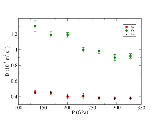
Figure 8: Self diffusion coefficients of Fe, Si and O atoms vs pressure for the Fe_0.79Si_0.08O_0.13 mixture. Temperatures are determined from the CORE5500 adiabat at the corresponding pressures.

References

- (1) J. P. Poirer, Phys. Earth Planet Int., 85, 319 (1994).
- (2) D. Alfè, M. J. Gillan and G. D. Price, Contemp. Phys. 48, 63 (2007).
- (3) R. N. Keeler and A. C. Mitchell, Solid State Commun., 7, 271 (1969).
- (4) R. N. Keeler and E. B. Royce, in Physics of High Energy Density, P. Caldirola amd H. Knoepfel eds., 106 (Proc. Int. Sch. Phys. Enrico Fermi Vol. 48, 1971).
- (5) W. M. Elsasser, Phys. Rev., 70, 202 (1946).
- (6) R. A. Secco and H. H. Schloessin, J. Geophys. Res., 94, 5887 (1989).
- (7) Y. Bi, H. Tan and F. Jing, J. Phys.: Condens. Matter, 14, 10849 (2002).
- (8) H. Gomi, K. Ohta and K. Hirose, American Geophysical Union, Fall Meeting 2010, abstract #MR23A-2012.
- (9) F. D. Stacey and O. L. Anderson, Phys. Earth Planet Int., 124, 153 (2001).
- (10) X. Sha and R. E. Cohen, J. Phys.: Condens. Matter, 23, 075401 (2011).
- (11) M. Pozzo, C. Davies, D. Gubbins and D. Alfè, Nature, 485, 355 (2012).
- (12) N. de Koker, G. Steinle-Neumann and V. Vlček, Proc. Natl. Acad. Sci., 109, 4070 (2012).
- (13) G. Matassov, The electrical conductivity of iron-silicon alloys at high pressure and the Earth’s core, PhD thesis, University of California (1977).
- (14) G. F. Davies, Phys. Earth Planet. Int., 160, 215 (2007).
- (15) F. D. Stacey and D. E. Loper, Phys. Earth Planet. Int., 161, 13 (2007).
- (16) Z. Konôpková, P. Lazor, A. F. Goncharov and V. V. Struzhkin, High Pressure Res., 31, 228 (2011).
- (17) D. Wiedemann, R. Franz, Annalen der Physik 89, 497 (1853).
- (18) G. Galli, R. M. Martin, R. Car, and M. Parrinello, Phys. Rev. Lett., 63, 988 (1989).
- (19) J. M. Holender, M. J. Gillan, M. C. Payne, A. D. Simpson, Phys. Rev. B, 52, 967 (1995).
- (20) P. L. Silvestrelli, A. Alavi and M. Parrinello, Phys. Rev. B, 55, 15515 (1997).
- (21) K. V. Tretiakov and S. Scandolo, J. Chem. Phys., 10, 3765 (2004).
- (22) V. Recoules and J.-P. Crocombette, Phys. Rev. B, 72, 104202 (2005).
- (23) F. Knider, J. Huger and A. V. Postnikov, J. Phys.:Condens. Matter, 19, 196105 (2007).
- (24) M. A. Morales, E. Schwegler, D. Ceperley, C. Pierleoni, S. Hamel, and K. Caspersen, Proc. Natl. Acad. Sci., 106, 1324 (2009).
- (25) M. A. Morales, C. Pierleoni, E. Schwegler, and D. M. Ceperley, Proc. Natl. Acad. Sci., 107, 12799 (2010).
- (26) W. Lorenzen, B. Holst, and R. Redmer, Phys. Rev. B, 84, 235109 (2011).
- (27) V. Vlček, N. de Koker, and G. Steinle-Neumann, Phys. Rev. B, 85, 184201 (2012).
- (28) M. French, T. R. Mattsson, and R. Redmer, Phys. Rev. B., 82, 174108 (2010).
- (29) K. Hirose, H. Gomi, K. Ohta, S. Labrosse and J. Hernlund, Mineral Mag., 75, 1027 (2011).
- (30) H. Gomi, K. Ohta, K. Hirose, S. Labrosse, J. W. Hernlund, R. Caracas, American Geophysical Union, Fall Meeting 2011, abstract #MR41B-2101.
- (31) H. Gomi, K. Ohta, K. Hirose, S. Labrosse, R. Caracas, M. J. Verstraete, J. W. Hernlund, Japan Geoscience Union Meeting 2012, abstract SIT41-P14.
- (32) G. Kresse and J. Furthmuller, Comp. Mater. Sci. 6, 15 (1996).
- (33) P. E. Blöchl, Phys. Rev. B 50, 17953 (1994).
- (34) G. Kresse and D. Joubert, Phys. Rev. B 59, 1758 (1999).
- (35) Y. Wang and J. P. Perdew, Phys. Rev. B 44, 13298 (1991); J. P. Perdew, J. A. Chevary, S. H. Vosko, K. A. Jackson, M. R. Pederson, D. J. Singh and C. Fiolhais, Phys. Rev. B 46, 6671 (1992).
- (36) D. Alfè, Comp. Phys. Comm. 118, 31 (1999).
- (37) H. C. Andersen, J. Chem. Phys. 72, 2384 (1980).
- (38) M. P. Desjarlais, J. D. Kress, and L. A. Collins, Phys. Rev. E, 66, 025401 (2002).
- (39) H. J. Monkhorst and J. D. Pack, Phys. Rev. B 13, 5188 (1976).
- (40) D. Alfè, M. Pozzo and M. P. Desjarlais, Phys. Rev. B 85, 024102 (2012).
- (41) C. Kittel, Introduction to solid state physics, 7th edition, John Wiley and Sons, Inc., New York (1996).
- (42) G. V. Chester and A. Thellung, Proc. Phys. Soc. London 77, 1005 (1961).
- (43) S. Mazevet, M. Torrent, V. Recoules, F. Jollet, High En. Den. Phys. 6, 84 (2010).
- (44) D. Alfè, G. D. Price, and M. J. Gillan, Phys. Rev. B, 65, 165118 (2002).
- (45) D. Alfè, Phys. Rev. B 79, 060101 (2009).
- (46) D. Alfè, M. J. Gillan and G. D. Price, Earth Planet Sci. Lett. 195, 91 (2002).
- (47) A. M. Dziewonski and D. L. Anderson, Phys. Earth Planet. Inter. 25, 297 (1981).
- (48) G. Masters and D. Gubbins, Phys. Earth Planet Int. 140, 159 (2003).
- (49) F. D. Murnaghan, Proc. Natl. Acad. Sci. 30, 244 (1944); F. Birch, Phys. Rev. 71, 809 (1947).
- (50) D. Alfè, G. D. Price, and M. J. Gillan, Phys. Earth. Planet. Int. 110, 191 (1999).
- (51) M. P. Allen, D. J. Tildesley, in Computer Simulation of Liquids Clarendon Press, Oxford (1987).
- (52) D. Alfè and M. J. Gillan, Phys. Rev. Lett. 81, 5161 (1998).
- (53) G. A. de Wijs, G. Kresse, L. Vočadlo, D. Dobson, D. Alfè, M. J. Gillan, G. D. Price, Nature 392, 805 (1998).
- (54) D. Alfè, G. Kresse and M. J. Gillan, Phys. Rev. B 61, 132 (2000).
- (55) E. Knittle, R. Jeanloz, A. C. Mitchell and W. J. Nellis, Solid State Commun., 59, 513 (1986).
- (56) F. Nimmo, Treatise on Geophysics, 8, 217 (2007).
- (57) F. Stacey, Encyclopedia of Geomagnetism and Paleomagnetism, 91 (2007).
- (58) S. Labrosse, J.-P. Poirier, and J.-L. Le Moeul, Earth Planet. Sci. Lett. 190, 111 (2001).
- (59) D. E. Loper, Geophys. J. Int., 54, 389 (1986).
- (60) D. Gubbins, B. Sreenivasan, J. Mound and S. Rost, Nature, 473, 361 (2011).
- (61) R. Holme, Treatise on Geophysics, 8, 107 (2007).
- (62) D. Gubbins, Geophys. J. Int., 137, 513 (1986).
- (63) D. Gubbins, Encyclopedia of Geomagnetism and Paleomagnetism, 287 (2007).