Quantum Degenerate Fermi Gas with Spin-orbit Coupling and Crossed Zeeman Fields

Abstract

We study quantum degenerate ultra-cold Fermi gases in the presence of artificial spin-orbit coupling and crossed Zeeman fields. We emphasize the case where parity is violated in the excitation spectrum and compare it with the simpler situation where parity is preserved. We investigate in detail spectroscopic properties such as the excitation spectrum, the spectral function, momentum distribution and density of states for the cases where parity is preserved or violated. Similarly, we show that thermodynamic properties such as pressure, chemical potential, entropy, specific heat, isothermal compressibility and induced spin polarization become anisotropic as a function of Zeeman field components, when parity is violated. Lastly, we discuss the effects of interactions and present results for the pairing temperature as the precursor for the transition to a superfluid state. In particular, we find that the pairing temperature is dramatically reduced in the weak interaction regime as parity violation gets stronger, and that the momentum dependence of the order parameter for superfluidity violates parity when crossed Zeeman fields are present for finite spin-orbit coupling.

I Introduction

The study of quantum degenerate fermions has been in the forefront of research in ultra-cold atoms and molecules in recent years, where particular attention was paid to the so-called evolution from BCS to BEC superfluidity. Bringing ultra-cold fermions into quantum degeneracy and using Feshbach resonances to tune interactions between colliding fermions opened the door for the exploration of their superfluid phases, and their thermodynamic and correlation properties. This ability to tune interactions and explore the limits of weak, strong and unitary interactions had impact not only in cold-atom physics, but also in condensed matter physics (strongly correlated superconductors), nuclear physics (superconductivity in quantum chromodynamics) and astrophysics (superfluidity in neutron stars).

Many advances in cold atoms followed after the development of new tools for their toolbox. For instance the experimental study of the evolution from BCS to BEC superfluidity occurred after appropriate Feshbach resonances for ⁶Li and ⁴⁰K were identified, and used to study the crossover problem for $s$-wave superfluids. In addition to $s$-wave Feshbach resonances, both ⁶Li and ⁴⁰K also exhibit $p$-wave Feshbach resonances, which could produce p-wave superfluids in particular in BEC regime if $p$-wave Feshbach molecules were stable. Unfortunately, such $p$-wave molecules do not live sufficiently long for the creation of $p$-wave superfluids jin-2007 ; mukaiyama-2008 ; vale-2008 ; zimmermann-2010 .

In addition to the manipulation of interactions, it has been possible to extract experimentally detailed thermodynamic information of interacting ultra-cold fermions salomon-2010 ; zwierlein-2012a from local density images of trapped atoms with the help of the local density approximation yip-2007 ; ho-2009 .

A further tool was developed recently through the production of tunable artificial spin-orbit fields spielman-2011 that were created in ⁸⁷Rb, a bosonic isotope of Rubidium, by using a set of Raman beams that allowed momentum transfer and mixing of two dressed spin states. In these experiments, the emergence of spin-orbit fields, controlled by the momentum transfer from the light fields to the atoms, was connected to the simultaneous existence of an artificial Zeeman field controlled by the Raman coupling. In such experiments, the artificial spin-orbit and Zeeman fields were used to manipulate the effective interactions between bosons and thus produce new quantum phases of bosonic matter spielman-2011 . In a subsequent experiment it was directly demonstrated that the effective interactions between bosons can acquire higher angular momentum components which are directly controlled by the artificial spin-orbit and Zeeman fields. The effective single-atom Hamiltonian created in these experiments is

$${\bf H}_{\rm sa}({\bf k})=\epsilon_{\bf k}{\bf 1}-h_{\parallel}\sigma_{z}-h_{x}({\bf k})\sigma_{x}-h_{y}({\bf k})\sigma_{y},$$ (1)

when expressed in the dressed state spin basis $|{\bf k},s\rangle$. Here, $\epsilon_{\bf k}={\bf k}^{2}/(2m)$ represents the kinetic energy of an atom with momentum ${\bf k}$ and spin state $s$, $h_{\parallel}=h_{z}=\Omega/2$ represents the Zeeman field along the quantization axis $z$ which is directly related to the Raman coupling $\Omega$, $h_{x}({\bf k})=0$ and $h_{y}({\bf k})=h_{y}+vk_{x}$, where $h_{y}=\delta/2$ represents the detuning and $vk_{x}$ represents a mixture of equal Rashba rashba-1960 and Dresselhaus dresselhaus-1955 terms, which we label as ERD spin-orbit coupling.

The possibility of studying similar phenomena with ultra-cold fermions in the presence of spin-orbit coupling and Zeeman fields spielman-2011 ; sademelo-2011 lead to an explosion of theoretical research, which focused primarily on the case of Rashba-only (RO) spin-orbit coupling shenoy-2011 ; chuanwei-2011 ; zhai-2011 ; hu-2011 ; iskin-2011 which has been studied extensively in condensed matter physics in the context of non-centro-symmetric superconductors gorkov-2001 ; yip-2002 ; sigrist-2004 . Some suggestions of possible realizations of artificial RO spin-orbit fields in ultra-cold fermions have appeared in the literature chuanwei-2008 ; sinova-2009 . However, in our group, we have focused mostly on the ERD case han-2012 ; seo-2012a ; seo-2011 ; seo-2012b , which is simpler to be realized experimentally as it was demonstrated for interacting bosons spielman-2011 ; sademelo-2011 in the case of ⁸⁷Rb, and more recently for non-interacting fermions such as ⁴⁰K in China zhang-2012 and ⁶Li in the United States zwierlein-2012b .

In our recent work han-2012 ; seo-2012a ; seo-2011 ; seo-2012b , we emphasized the importance of interactions in producing novel phases for spin-orbit coupled ultra-cold fermions in the presence of Zeeman fields, and we analyzed in detail the ERD case with a longitudinal Zeeman field which is orthogonal to the spin-orbit field seo-2012a ; seo-2011 ; seo-2012b . In this paper, we generalize our previous analysis to include an additional Zeeman field $h_{y}$ representing the detuning $\delta$, which is perpendicular to longitudinal Zeeman field $h_{\parallel}=h_{z}$ representing the Raman coupling $\Omega$. In this case, the simultaneous presence of $h_{y}$ and the ERD spin-orbit field $vk_{x}$ along the $y$ axis leads to the loss of parity for the eigenvalues of $H_{\rm sa}({\bf k})$ defined in Eq. (1) above. This violation of parity in the energy spectrum leads to many detectable parity-violating properties in spectroscopic quantities such as the spectral function and momentum distribution, which are explicitly momentum-dependent, or in momentum-integrated quantities like the density of states when viewed as a function of Zeeman fields $h_{y}$ and $h_{y}$. Furthermore, we demonstrate that this parity violation can also be seen and quantified in thermodynamic quantities such as the pressure, entropy, specific heat, chemical potential, compressibility and spin-polarization, which are discussed in detail for non-interacting ultra-cold fermions in the presence of ERD spin-orbit and crossed Zeeman fields $h_{y}$ and $h_{z}$. Furthermore, we also discuss the effects of parity violation when attractive $s$-wave interactions are present, and we pay particular attention to the pairing temperature and to the absence of parity in the order parameter tensor describing the superfluid order.

The remainder of the paper is as follows. In section II, we describe the magnetic hamiltonian in its general form, and particularize it to any linear combination of Rashba and Dresselhaus terms, while in section III we discuss the independent-atom (non-interacting) Hamiltonian including both the kinetic energy and the magnetic parts. The eigenvalues and eigenvectors of the single-atom Hamiltonian are discussed in section IV, where a generalized helicity basis is introduced and Fermi surfaces for various values of crossed Zeeman fields are presented. Particular attention is paid to parity violations for the eigenvalues and eigenvectors. In section V, we show the momentum dependence for the spectral function at fixed frequency revealing the cases of weak and strong parity violations, while in section VI we describe the the spin-resolved momentum distributions which also reveal parity violations for various values of crossed Zeeman fields. In section VII, we analyze the spin-dependent density of states for a few values of the crossed Zeeman fields and fixed ERD spin-orbit coupling, while in section VIII, we define several thermodynamics properties which analyzed in the following sections, such as pressure and entropy in section IX, chemical potential in section X, isothermal compressibility in section XI and spin-polarization XII. Furthermore, we investigate the effects of parity violation on the effective interactions in section XIII and on the pairing temperature in section XV. Lastly, we state our conclusions in section XVI emphasizing that several measurements can be made to detect parity violation in both non-interacting and interacting Fermi gases in the simultaneous presence of an ERD spin-orbit field, and crossed Zeeman fields $h_{y}$, $h_{z}$, where $h_{y}$ is related to the detuning $\delta$ and $h_{z}$ to Raman coupling $\Omega$.

II Magnetic Hamiltonian

To describe quantum degenerate Fermi systems in the presence of artificial spin-orbit and crossed artificial Zeeman fields, we discuss first the type of magnetic Hamiltonian to be used. Generally speaking the coupling between magnetic fields and two spin-states is given by $H_{\rm mag}({\bf k})=-h({\bf k})\cdot\bm{\sigma},$ where ${\bf h}({\bf k})$ is the effective magnetic field (including Zeeman and spin-orbit) and $\bm{\sigma}=(\sigma_{x},\sigma_{y},\sigma_{z})$, with $\sigma_{i}$ being the Pauli matrices. This leads to the magnetic Hamiltonian

$$H_{\rm mag}({\bf k})=\begin{pmatrix}h_{z}({\bf k})&h_{x}({\bf k})-ih_{y}({\bf k})\\ h_{x}({\bf k})+ih_{y}({\bf k})&-h_{z}({\bf k})\end{pmatrix}.$$ (2)

Although there are many possible forms of fictitious magnetic fields that can be created in the laboratory. We discuss here a few simpler magnetic field configurations. In principle, the external artificial Zeeman field ${\bf h}_{\rm ZE}$ can have three components $(h_{x},h_{y},h_{z})$, in practice, we set $h_{x}=0$, and $(h_{y},h_{z})\neq 0$ because in current experimental setups $h_{y}=\delta/2$, where $\delta$ is the laser detuning, and $h_{z}=\Omega/2$, where $\Omega$ is the strength of Raman coupling field.

In addition, there are many possible types of spin-orbit contributions where ${\bf h}_{SO}$ can have three components $\left(h_{SO,x}({\bf k}),h_{SO,y}({\bf k}),h_{SO,z}({\bf k})\right)$. However, we consider particular forms of spin-orbit fields, which can be more easily realized in practice. The first type has the Dresselhaus form ${\bf h}_{D}({\bf k})=v_{D}\begin{pmatrix}k_{y},&k_{x},&0\end{pmatrix},$ where $v_{D}$ measures the strength of the Dresselhaus field in units of velocity. The corresponding Hamiltonian for such field is

$${\bf H}_{D}({\bf k})=-v_{D}\begin{pmatrix}0&k_{y}-ik_{x}\\ k_{y}+ik_{x}&0\end{pmatrix}.$$ (3)

The second type has the Rashba form ${\bf h}_{R}({\bf k})=v_{R}\begin{pmatrix}-k_{y},&k_{x},&0\end{pmatrix},$ where $v_{R}$ measures the strength of the Rashba field in units of velocity. The corresponding Rashba Hamiltonian is

$${\bf H}_{R}({\bf k})=v_{R}\begin{pmatrix}0&k_{y}+ik_{x}\\ k_{y}-ik_{x}&0\end{pmatrix}.$$ (4)

Either the Dresselhaus or the Rashba forms require spin-orbit fields along the $x$ and $y$ directions, which to be produced experimentally demand two orthogonal Raman setups, such that momentum transfer occurs in two perpendicular directions. A linear combination of two forms leads to the field ${\bf h}_{RD}({\bf k})=\begin{pmatrix}v_{RD_{-}}k_{y},&v_{RD_{+}}k_{x},&0\end{pmatrix},$ where the velocities $v_{RD_{\pm}}=(v_{D}\pm v_{R}).$ The corresponding Hamiltonian for such linear combination is

$${\bf H}_{RD}({\bf k})=\begin{pmatrix}0&v_{RD_{-}}k_{y}+iv_{RD_{+}}k_{x}\\ v_{RD_{-}}k_{y}-iv_{RD_{+}}k_{x}&0\end{pmatrix}.$$ (5)

The simplest type of spin-orbit field that can been created in the laboratory has the equal-Rashba-Dresselhaus (ERD) form ${\bf h}_{ERD}({\bf k})=v(0,k_{x},0),$ where $v_{RD_{-}}=0$, and $v_{RD_{+}}=v$, or equivalently $v_{D}=v_{R}=v/2$. The corresponding Hamiltonian for the ERD spin-orbit field has the simple form

$${\bf H}_{ERD}({\bf k})=v\begin{pmatrix}0&ik_{x}\\ -ik_{x}&0\end{pmatrix}.$$ (6)

Taking into account an arbitrary superposition of Rashba and Dresselhaus spin-orbit coupling and a general uniform Zeeman field ${\bf h}_{ZE}=\left(h_{x},h_{y},h_{z}\right)$, we can write the Zeeman-spin-orbit Hamiltonian as

$${\bf H}_{ZSO}({\bf k})=-\begin{pmatrix}h_{\parallel}&h_{\perp}({\bf k})\\ h_{\perp}^{*}({\bf k})&-h_{\parallel}\end{pmatrix},$$ (7)

where the parallel component of the total field is $h_{\parallel}=h_{z}$ and the transverse component is

$$h_{\perp}({\bf k})=\left[h_{x}+h_{RD,x}({\bf k})-i(h_{y}+h_{RD,y}({\bf k})\right],$$

where $h_{RD,x}({\bf k})=v_{RD_{-}}k_{y}$ and $h_{RD,y}({\bf k})=v_{RD_{+}}k_{x}.$

Having presented the magnetic Hamiltonian, we discuss next the Hamiltonian including the kinetic energy of the atoms.

III Hamiltonian

The Hamiltonian for non-interacting ultra-cold fermions with identical masses $m$ in the presence of spin-orbit and crossed Zeeman fields can be written in second quantization as

$$\mathcal{H}=\sum_{\bf k}\Psi^{\dagger}({\bf k}){\bf H}({\bf k})\Psi({\bf k}),$$ (8)

where the spinor $\Psi^{\dagger}({\bf k})=\left(c_{{\bf k}\uparrow}^{\dagger},c_{{\bf k}\downarrow}^{\dagger}\right)$ describes the creation of fermion states with momentum ${\bf k}$ and spin $\uparrow$ or $\downarrow$. Such Hamiltonian describes two hyperfine states of Fermi atoms such as ${}^{6}{\rm Li}$ or ${}^{40}{\rm K}$, and the corresponding Hamiltonian matrix is

$${\bf H}({\bf k})=\begin{pmatrix}{\widetilde{K}}_{\uparrow}({\bf k})&-h_{\perp}({\bf k})\\ -h_{\perp}^{*}({\bf k})&{\widetilde{K}}_{\downarrow}({\bf k})\end{pmatrix},$$ (9)

where ${\widetilde{K}}_{\sigma}({\bf k})=k^{2}/(2m)-\mu_{\sigma}$ represents the kinetic energy of a fermion with mass $m$, momentum ${\bf k}$ and spin $\sigma$ with respect to the chemical potential $\mu_{\sigma}$.

We define the variables ${\widetilde{K}}_{\pm}=\left({\widetilde{K}}_{\uparrow}\pm{\widetilde{K}}_{\downarrow}\right)/2$ and the chemical potentials $\mu_{\pm}=\left(\mu_{\uparrow}\pm\mu_{\downarrow}\right)/2,$ and notice that ${\widetilde{K}}_{+}=|{\bf k}|^{2}/(2m)-\mu_{+}=\xi_{{\bf k}+}$ plays the role of the average kinetic energy, while ${\widetilde{K}}_{-}=-(\mu_{-}+h_{z})\equiv-h_{\parallel},$ plays the role of the parallel Zeeman field $h_{\parallel}$ including the external field $h_{z}$ and the internal field $\mu_{-}$ due to a possible initial population imbalance. In the limit that there is zero initial population imbalance, the chemical potentials can be set to $\mu_{+}\to\mu$ and $\mu_{-}\to 0$, while the kinetic energies reduce to ${\widetilde{K}}_{+}({\bf k})\to\xi_{\bf k}$ and ${\widetilde{K}}_{-}({\bf k})\to-h_{\parallel}=-h_{z}$, where $\xi_{\bf k}=|{\bf k}|^{2}/(2m)-\mu$.

The non-interacting Hamiltonian has the simpler form ${\bf H}_{0}({\bf k})=\xi_{\bf k}{\bf 1}-h_{\parallel}\sigma_{z}-h_{x}({\bf k})\sigma_{x}-h_{y}({\bf k})\sigma_{y}$ which can be re-expressed as

$${\bf H}_{0}({\bf k})=\begin{pmatrix}\xi_{\bf k}-h_{\parallel}&-h_{\perp}({\bf k})\\ -h_{\perp}^{*}({\bf k})&\xi_{\bf k}+h_{\parallel}\end{pmatrix},$$ (10)

where $h_{\perp}({\bf k})=h_{x}({\bf k})-ih_{y}({\bf k}).$ In the remainder of the manuscript, we will discuss this explicit form of the Hamiltonian and some interesting consequences.

We define the total number of fermions as $N=N_{\uparrow}+N_{\downarrow}$, and choose our energy, velocity and momentum scales through the Fermi momentum $k_{F}$ defined from the total density of fermions $n=n_{\uparrow}+n_{\downarrow}=k_{F}^{3}/(3\pi^{2}),$ where $n=N/V$ and $n_{s}=N_{s}/V$ with $s=(\uparrow,\downarrow)$. This choice leads to the Fermi energy $\epsilon_{F}=k_{F}^{2}/2m$ and to the Fermi velocity $v_{F}=k_{F}/m$, which are the energy and velocity scales used throughout the manuscript.

IV Excitation Spectrum

Now, let us introduce the unitary matrix ${\bf U}_{\bf k}$ that diagonalizes the Hamiltonian ${\bf H_{0}}({\bf k})$, such that

$${\bf E}({\bf k})={\bf U}^{\dagger}_{\bf k}{\bf H}_{0}({\bf k}){\bf U}_{\bf k}$$ (11)

is a diagonal matrix containing the eigenvalues of ${\bf H}_{0}({\bf k})$. The corresponding eigenvectors are the spinors $\Phi({\bf k})={\bf U}_{\bf k}^{\dagger}\Psi({\bf k}),$ where the unitary matrix ${\bf U}_{\bf k}$ has a momentum-dependent SU(2) form and can be written as

$${\bf U}_{\bf k}=\begin{pmatrix}u_{\bf k}&v_{\bf k}\\ -v^{*}_{\bf k}&u_{\bf k}\end{pmatrix},$$ (12)

where the normalization condition $|u_{\bf k}|^{2}+|v_{\bf k}|^{2}=1$ is imposed to satisfy the unitarity condition ${\bf U}_{\bf k}^{\dagger}{\bf U}_{\bf k}={\bf 1}$ leading to the following expressions

$$u_{\bf k}=\sqrt{\frac{1}{2}\left(1+\frac{h_{\parallel}}{\lvert{\bf h}_{{\rm eff}}({\bf k})\rvert}\right)},$$ (13)

where $u_{\bf k}$ is taken to be real without loss of generality and

$$v_{\bf k}=-e^{i\varphi_{\bf k}}\sqrt{\frac{1}{2}\left(1-\frac{h_{\parallel}}{\lvert{\bf h}_{\rm{eff}}({\bf k})\rvert}\right)},$$ (14)

is a complex function where the phase $\varphi_{\bf k}$ is defined via $h_{\perp}({\bf k})=|h_{\perp}({\bf k})|e^{i\varphi_{\bf k}},$ leading to $\varphi_{\bf k}={\rm Arg}\left[h_{\perp}({\bf k})\right]$ .

The eigenvalues of ${\bf H}_{0}({\bf k})$ emerge as

$${\bf E}({\bf k})=\begin{pmatrix}\xi_{\Uparrow}({\bf k})&0\\ 0&\xi_{\Downarrow}({\bf k})\end{pmatrix},$$ (15)

where $\xi_{\Uparrow}({\bf k})=\xi_{k}-\lvert{\bf h}_{\rm eff}({\bf k})\rvert$ is the eigenvalue where the momentum dependent effective field ${\bf h}_{\rm eff}({\bf k})$ is aligned with the spin $\Uparrow$, and $\xi_{\Downarrow}({\bf k})=\xi_{\bf k}+\lvert{\bf h}_{\rm eff}({\bf k})\rvert$ is the eigenvalue where the momentum dependent effective field ${\bf h}_{\rm eff}({\bf k})$ is aligned with the spin $\Downarrow$. Here, $\lvert{\bf h}_{\rm eff}({\bf k})\rvert=\sqrt{h_{\parallel}^{2}+\lvert h_{\perp}({\bf k})\rvert^{2}}$ is the magnitude of the effective field. The respective eigenvectors are

$$\Phi_{\Uparrow}({\bf k})=u_{{\bf k}}c_{{\bf k}\uparrow}-v_{{\bf k}}c_{{\bf k}\downarrow}$$ (16)

corresponding to the state $|{\bf k},\Uparrow\rangle$, and

$$\Phi_{\Downarrow}({\bf k})=v_{{\bf k}}^{*}c_{{\bf k}\uparrow}+u_{{\bf k}}c_{{\bf k}\downarrow}$$ (17)

corresponding to the state $|{\bf k},\Downarrow\rangle$.

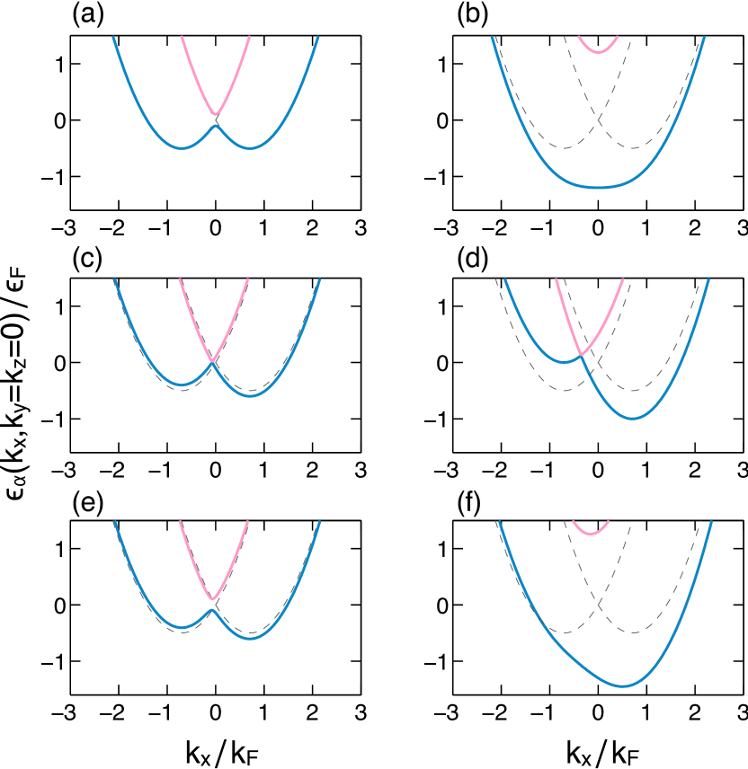
Figure 1: (color online) Helicity energy dispersions $\epsilon_{\Uparrow}({\bf k})/\epsilon_{F}$ (blue line) and $\epsilon_{\Downarrow}({\bf k})/\epsilon_{F}$ (magenta line) versus momentum $k_{x}/k_{F}$ with $k_{y}=k_{z}=0$ for ERD spin-orbit coupling $v/v_{F}=0.71$. For reference, the black dashed lines show the helicity bands for $v/v_{F}=0.71$ with $h_{z}/\epsilon_{F}=h_{y}/\epsilon_{F}=0$. The Zeeman fields are (a) $h_{y}/\epsilon_{F}=0$ and $h_{z}/\epsilon_{F}=0.1$, (b) $h_{y}/\epsilon_{F}=0$ and $h_{z}/\epsilon_{F}=1.2$, (c) $h_{y}/\epsilon_{F}=0.1$ and $h_{z}/\epsilon_{F}=0$, (d) $h_{y}/\epsilon_{F}=0.5$ and $h_{z}/\epsilon_{F}=0$, (e) $h_{y}/\epsilon_{F}=h_{z}/\epsilon_{F}=0.1$, (f) $h_{y}/\epsilon_{F}=0.5$ and $h_{z}/\epsilon_{F}=1.2$.

For initially population balanced systems in the ERD case, with the Zeeman field having only $h_{y}$ and $h_{z}$ components, the magnitude of the effective magnetic field $|h_{\rm eff}({\bf k})|=\sqrt{h_{z}^{2}+\left(h_{y}+vk_{x}\right)^{2}}$ does not have well defined parity, which implies that the same is true for the eigenvalues $\xi_{\alpha}({\bf k})$. If either $h_{y}=0$ (zero detuning) or $v=0$ (zero spin-orbit coupling), parity is restored for the eigenvalues. This can be seen in Fig. 1, where the energy dispersions $\epsilon_{\Uparrow}({\bf k})=\epsilon_{\bf k}-|h_{\rm eff}({\bf k})|$ and $\epsilon_{\Downarrow}({\bf k})=\epsilon_{\bf k}+|h_{\rm eff}({\bf k})|$ are shown for several cases. In all panels of Fig. 1 the dashed lines represent the case where the ERD spin orbit is finite $(v/v_{F}=0.71)$, but the Zeeman fields are zero $(h_{z}=h_{y}=0)$. This case corresponds to shifted parabolic bands $\epsilon_{\Uparrow}({\bf k})=k_{x}^{2}/(2m)-|vk_{x}|+k_{\rho}^{2}/(2m)$ and $\epsilon_{\Downarrow}({\bf k})=k_{x}^{2}/(2m)+|vk_{x}|+k_{\rho}^{2}/(2m),$ where $k_{\rho}^{2}=k_{y}^{2}+k_{z}^{2}$. The lower helicity band $\epsilon_{\Uparrow}({\bf k})$ has two minima, which occur at $(k_{x}=m|v|,k_{y}=0,k_{z}=0)$ and $(k_{x}=-m|v|,k_{y}=0,k_{z}=0)$, respectively, while the upper helicity band $\epsilon_{\Uparrow}({\bf k})$ has only one minimum occurring at $(k_{x}=0,k_{y}=0,k_{z}=0)$. This can be seen by completing the squares and rewriting the dispersions of the helicity bands as $\epsilon_{\Uparrow}({\bf k})=(|k_{x}|-m|v|)^{2}/(2m)-\epsilon_{v}+k_{\rho}^{2}/(2m)$ and $\epsilon_{\Downarrow}({\bf k})=(|k_{x}|+m|v|)^{2}/(2m)-\epsilon_{v}+k_{\rho}^{2}/(2m),$ where $\epsilon_{v}=mv^{2}/2$ is the characteristic kinetic energy associated with the spin-orbit coupling strength $v$, which has units of velocity.

In Fig. 1a, we show the case of $v/v_{F}=0.71$, for $h_{y}=0$ and $h_{z}/\epsilon_{F}=0.1$, and in Fig. 1b, we show the case of $v/v_{F}=0.71$, for $h_{y}=0$ and $h_{z}/\epsilon_{F}=1.2$. In both of these cases the energy dispersions are parity preserving, and the main fundamental difference between Fig. 1a and Fig. 1b is that the lower helicity band $\epsilon_{\Uparrow}({\bf k})$ has two minima at finite $k_{x}=\pm|v|^{-1}\sqrt{4\epsilon_{v}^{2}-h_{z}^{2}}$ as seen in Fig. 1a, but a single minimum at $k_{x}=0$ as seen in Fig. 1b. While the upper helicity band $\epsilon_{\Downarrow}({\bf k})$ has only a single minimum at $k_{x}=0$ in both Fig. 1a and Fig. 1b. The two minima in the lower helicity band for Fig. 1a occur only for low Zeeman fields $|h_{z}|<2\epsilon_{v}$. In Figs. 1c and 1d, we show the helicity bands for $h_{z}=0$, but $h_{y}/\epsilon_{F}=0.1$ and $h_{y}/\epsilon_{F}=0.5$, respectively. In these cases, the energy dispersions are $\epsilon_{\Uparrow}({\bf k})=k_{x}^{2}/(2m)-|h_{y}+vk_{x}|+k_{\rho}^{2}/(2m)$ and $\epsilon_{\Downarrow}({\bf k})=k_{x}^{2}/(2m)+|h_{y}+vk_{x}|+k_{\rho}^{2}/(2m)$ and do not even parity as it is standard, since $\epsilon_{\alpha}({\bf k})\neq\epsilon_{\alpha}(-{\bf k}).$ These dispersions are compared to the dispersions for the case of $h_{y}/\epsilon_{F}=h_{z}/\epsilon_{F}=0$, but finite $v/v_{F}$, which are shown as dashed black lines in Fig. 1. The last examples described in Fig. 1e and Fig. 1f correspond to cases where both $h_{y}$ and $h_{z}$ are non-zero, having values $h_{y}/\epsilon_{F}=h_{z}/\epsilon_{F}=0.1$ for (e) and $h_{y}/\epsilon_{F}=0.5$, $h_{z}/\epsilon_{F}=1.2$ for (f). Notice the presence of two minima for the lower helicity band in (e), and the existence of only one minimum for the lower helicity band in (f), but in both cases parity (inversion symmetry) is violated.

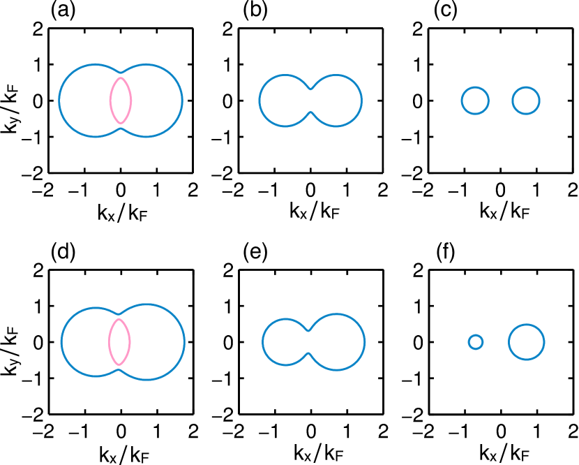
Figure 2: (color online) Cross sections of Fermi surfaces in the $k_{x}$-$k_{y}$ plane at $k_{z}=0$ for ERD spin-orbit coupling $v/v_{F}=0.71$. In (a) through (c), the Zeeman fields are $h_{y}/\epsilon_{F}=0$ and $h_{z}/\epsilon_{F}=0.1$, where parity symmetry is preserved, and the different values of the chemical potential and induced polarization are (a) $\mu/\epsilon_{F}=0.495$, $P_{\rm ind}=0.121$, (b) $\mu/\epsilon_{F}=0$, $P_{\rm ind}=0.147$, (c) $\mu/\epsilon_{F}=-0.370$, $P_{\rm ind}=0.106$. In (d) through (f) the Zeeman fields are $h_{y}/\epsilon_{F}=h_{z}/\epsilon_{F}=0.1$, where parity symmetry is not preserved, and the different values of the chemical potential and induced polarization are (d) $\mu/\epsilon_{F}=0.492$, $P_{\rm ind}=0.121$, (e) $\mu/\epsilon_{F}=0$, $P_{\rm ind}=0.143$, (f) $\mu/\epsilon_{F}=-0.370$, $P_{\rm ind}=0.100$. The blue and magenta lines indicate the energy contours of the lower $\epsilon_{\Uparrow}({\bf k})$ and upper $\epsilon_{\Uparrow}({\bf k})$ helicity bands, respectively.

In Fig. 2, we show cross sections of the Fermi surfaces (FS) in the $k_{x}$-$k_{y}$ plane at $k_{z}=0$ for ERD spin-orbit coupling and a few values of crossed Zeeman fields. The Fermi surfaces have rotational symmetry about the $k_{x}$ axis, that is, in the $k_{y}$-$k_{z}$ plane, and their full three-dimensional structure can be visualized using this property. We show in Figs. 2a-c the case for Zeeman fields $h_{y}/\epsilon_{F}=0$ and $h_{z}/\epsilon_{F}=0.1$, where the Fermi surfaces exhibit parity (or inversion) symmetry. These parameters correspond to the helicity bands shown in Fig. 1a, where the lower helicity band has two minima. While we show in Figs. 2d-f the case for Zeeman fields $h_{y}/\epsilon_{F}=h_{z}/\epsilon_{F}=0.1$, where the corresponding Fermi surfaces do not have well defined parity or inversion symmetry. The specific values of the chemical potential $\mu$ and induced polarization $P_{\rm ind}=(N_{\uparrow}-N_{\downarrow})/(N_{\uparrow}+N_{\downarrow})$ are indicated in the captions.

In Fig. 2, notice also that as the chemical potential $\mu$ is changed below the bottom of the helicity band $\epsilon_{\Downarrow}({\bf k})$, the central pocket of the Fermi surface disappears (see magenta surface near zero momentum in Fig. 2). Further lowering of the chemical potential leads to the crossing of a local maximum of the helicity band $\epsilon_{\Uparrow}({\bf k})$, where the residual Fermi surface break into two pockets (see blue surfaces in Fig. 2). This is reminiscent of the Lifshitz transition lifshitz-1960 in non-interacting metals, also called metal-to-metal or conductor-to-conductor transition, where under pressure or another external parameter the Fermi surface of the system changes topology producing a major rearrangement of momentum states which lead to a drastic change in the density of states of the system. The thermodynamic potential $\Omega$ in the vicinity of the usual Lifshitz transition behaves as $\Omega=\Omega_{\rm reg}+\alpha|\mu-\mu_{c}|^{5/2},$ where $\Omega_{\rm reg}$ is the regular (analytic) part, and $\alpha$ is the prefactor of the non-analytic component. The isothermal compressibility is related to the second-derivative of the thermodynamic potential with respect to the chemical potential and behaves as $\kappa_{T}=\kappa_{T,{\rm reg}}+\beta|\mu-\mu_{c}|^{1/2},$ where $\kappa_{T,{\rm reg}}$ is the regular part and $\beta$ is the coefficient of the non-analytic component. According to Ehrenfest’s classification of phase transitions, the non-analyticity manifests itself only in the third derivative and is a third-order phase transition. However, the Lifshitz transition is more commonly called the $2$-$1/2$ order transition in allusion to the specific $5/2$ power-law non-analyticity of $\Omega$ in three dimensions. This topological transition is not characterized under Landau’s symmetry-based classification, since no symmetry is broken in the Lifshitz case. This trivial Lifshitz transition can be seen in Fig. 2 both for the parity-preserving and parity-violating examples.

In Fig. 3, we also show cross sections of the Fermi surfaces (FS) in the $k_{x}$-$k_{y}$ plane at $k_{z}=0$ for ERD spin-orbit coupling $v/v_{F}=0.71$ and a few values of crossed Zeeman fields. The Fermi surfaces have also rotational symmetry about the $k_{x}$ axis, that is, in the $k_{y}$-$k_{z}$ plane. We show in Figs. 3a-b the case for Zeeman fields $h_{y}/\epsilon_{F}=0$ and $h_{z}/\epsilon_{F}=1.2$, where the Fermi surfaces exhibit parity (or inversion) symmetry. These parameters correspond to the helicity bands shown in Fig. 1b, where the lower helicity band has only one minimum. While we show in Figs. 3c-d the cases of the Zeeman fields $h_{y}/\epsilon_{F}=0.5$ and $h_{z}/\epsilon_{F}=1.2$ where the corresponding Fermi surfaces do not have well defined parity or inversion symmetry. The values of the chemical potential $\mu$ and induced polarization $P_{\rm ind}$ are $\mu/\epsilon_{F}=1.5$, $P_{\rm ind}=0.692$ for Fig. 3a; $\mu/\epsilon_{F}=0$, $P_{\rm ind}=0.801$ for Fig. 3b; $\mu/\epsilon_{F}=1.5$, $P_{\rm ind}=0.673$ for Fig. 3c; and $\mu/\epsilon_{F}=0$, $P_{\rm ind}=0.739$ for Fig. 3d. Notice that there is a fundamental difference between the Fermi surfaces in Figs. 2 and 3 in connection with their topology. The lower helicity band $\epsilon_{\Uparrow}({\bf k})$ can have two simply connected FS for the parameters of Fig. 2, but only one simply connected FS for the parameters of Fig. 3. This means that there is only one trivial Lifshitz transition in the case of Fig. 3, while there are two trivial Lifshitz transitions in the case of Fig. 2. We call this transition for non-interacting systems trivial to contrast it with a more exotic, but related topological transition that can occur in $p$-wave volovik-1992 ; botelho-2005a or $d$-wave duncan-2000 ; botelho-2005b superfluids, where interactions play a fundamental role.

A further characterization of the parity violation present in fermion systems with spin-orbit coupling and crossed Zeeman fields can be made by analyzing additional spectroscopic quantities such as the spectral function to be discussed next.

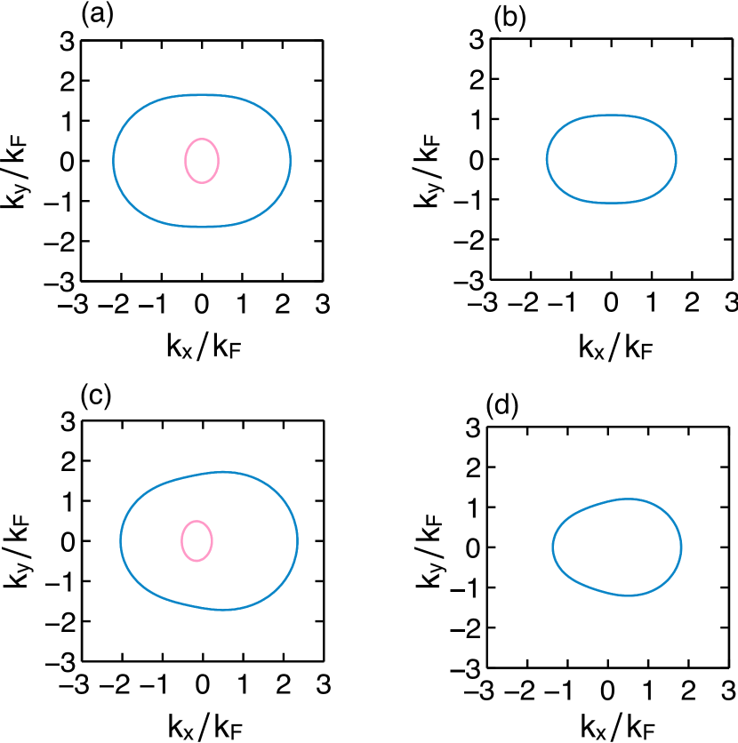
Figure 3: (color online) Cross sections of Fermi surfaces in the $k_{x}$-$k_{y}$ plane at $k_{z}=0$ for ERD spin-orbit coupling $v/v_{F}=0.71$. In (a) and (b), the Zeeman fields are $h_{y}/\epsilon_{F}=0$ and $h_{z}/\epsilon_{F}=1.2$, with parity symmetry being preserved. The values of the chemical potential and induced polarization are (a) $\mu/\epsilon_{F}=1.5$, $P_{\rm ind}=0.692$; (b) $\mu/\epsilon_{F}=0$, $P_{\rm ind}=0.801$. In (c) and (d), the Zeeman fields are $h_{y}/\epsilon_{F}=0.5$, $h_{z}/\epsilon_{F}=1.2$ and parity symmetry is not preserved. The values of the chemical potential and induced polarization are (c) $\mu/\epsilon_{F}=1.5$, $P_{\rm ind}=0.673$; (d) $\mu/\epsilon_{F}=0$, $P_{\rm ind}=0.739$. The blue and magenta lines indicate the energy contours of the lower $\epsilon_{\Uparrow}({\bf k})$ and upper $\epsilon_{\Uparrow}({\bf k})$ helicity bands, respectively.

V Spectral Function

A very useful tool to probe momentum-resolved properties is the use of radio-frequency (RF) spectroscopy that can extract the spectral function jin-2010 yielding similar measurements to those encountered in photoemission spectroscopy of condensed matter physics. The resolvent (or Green) operator matrix is defined as

$${\bf G}({\bf k},z)=\frac{1}{z{\bf 1}-{\bf H}({\bf k})}$$ (18)

in momentum-frequency space. In the present case, the diagonal components of ${\bf G}({\bf k},z)$ are

$$G_{\uparrow}({\bf k},z)=\frac{u_{\bf k}^{2}}{z-\xi_{\Uparrow}({\bf k})}+\frac{\lvert v_{\bf k}\rvert^{2}}{z-\xi_{\Downarrow}({\bf k})}$$ (19)

for the spin $\uparrow$ component and

$$G_{\downarrow}({\bf k},z)=\frac{\lvert v_{\bf k}\rvert^{2}}{z-\xi_{\Uparrow}({\bf k})}+\frac{u_{\bf k}^{2}}{z-\xi_{\Downarrow}({\bf k})}$$ (20)

for the spin $\downarrow$ component. The corresponding spectral function is $A_{s}({\bf k},\omega)=-\pi^{-1}{\rm{Im}}\left[G_{s}({\bf k},\omega+i\delta)\right],$ which in terms of the coherence factor $u_{\bf k}$ and $v_{\bf k}$ becomes

$$A_{\uparrow}({\bf k},\omega)=u_{\bf k}^{2}\delta(\omega-\xi_{\Uparrow}({\bf k}))+|v_{\bf k}|^{2}\delta(\omega-\xi_{\Downarrow}({\bf k}))$$ (21)

for the up-spin $({\uparrow})$ component, and

$$A_{\downarrow}({\bf k},\omega)=|v_{\bf k}|^{2}\delta(\omega-\xi_{\Uparrow}({\bf k}))+u_{\bf k}^{2}\delta(\omega-\xi_{\Downarrow}({\bf k}))$$ (22)

for the down-spin $(\downarrow)$ component.

The spectral functions $A_{s}({\bf k},\omega)$ at frequency $\omega=\mu$ and temperature $T/\epsilon_{F}=0.05$ are shown in Fig. 4 for some values of the crossed Zeeman fields and spin-orbit coupling. A small energy broadening $\delta/\epsilon_{F}=0.01$ is included and a logarithmic scale is used to help visualization. In the relevant panels of Fig. 4, the blue dashed lines represent $A_{s}(k_{x}=0,k_{y},k_{z}=0,\omega=\mu)$, and the red solid lines represent $A_{s}(k_{x},k_{y}=0,k_{z}=0,\omega=\mu)$. Additionally, the two left-most columns correspond to the $A_{\uparrow}({\bf k})$ component, and the two right-most columns describe the $A_{\downarrow}({\bf k})$ component. In Figs. 4(a)-(d) the Zeeman fields are $h_{y}/\epsilon_{F}=h_{z}/\epsilon_{F}=0$, the ERD coupling is $v/v_{F}=0$, the chemical potential is $\mu/\epsilon_{F}=1.0$, and the induced polarization $P_{\rm ind}=0$. In Figs. 4(e)-(h) the Zeeman fields are $h_{y}/\epsilon_{F}=0$, $h_{z}/\epsilon_{F}=0.1$, the ERD coupling is $v/v_{F}=0.71$, and the chemical potential is $\mu/\epsilon_{F}=0.495$, and the induced polarization is $P_{\rm ind}=0.121$. In these two cases parity is preserved, since the eigenvalues $\epsilon_{\alpha}({\bf k})$ and coherence factors $u_{\bf k}$ and $v_{\bf k}$ are invariant under momentum inversion for $h_{y}/\epsilon_{F}=0$. In Figs. 4(i)-(l) the Zeeman fields are $h_{y}/\epsilon_{F}=h_{z}/\epsilon_{F}=0.1$, the ERD coupling is $v/v_{F}=0.71$, the chemical potential is $\mu/\epsilon_{F}=0.492$, and the induced polarization is $P_{\rm ind}=0.120$. Parity is not preserved in the last case since $(h_{y}/\epsilon_{F}\neq 0$). This is reflected in the absence of inversion symmetry, which is noticeable but weak.

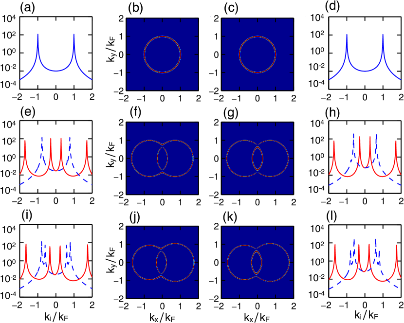
Figure 4: (color online) Finite temperature $(T/\epsilon_{F}=0.05)$ dimensionless spectral functions $2\pi\epsilon_{F}A_{s}({\bf k},\omega)$ at $\omega=\mu$ for parameters (a)-(d) $v/v_{F}=0$, $h_{y}/\epsilon_{F}=h_{z}/\epsilon_{F}=0$ and $\mu/\epsilon_{F}=1.0$; (e)-(h) $v/v_{F}=0.71$, $h_{y}/\epsilon_{F}=0$, $h_{z}/\epsilon_{F}=0.1$, and $\mu/\epsilon_{F}=0.495$; (i)-(l) $v/v_{F}=0.71$, $h_{y}/\epsilon_{F}=h_{z}/\epsilon_{F}=0.1$ and $\mu/\epsilon_{F}=0.492$. The blue dashed lines are cuts along the direction $(k_{x}=0,k_{y},k_{z}=0)$ corresponding to $2\pi\epsilon_{F}A_{s}(k_{x}=0,k_{y},k_{z}=0,\omega=\mu)$, and the red solid lines are cuts along the direction $(k_{x},k_{y}=0,k_{z}=0)$ corresponding to $2\pi\epsilon_{F}A_{s}(k_{x},k_{y}=0,k_{z}=0,\omega=\mu)$. The two left-most columns describe the $A_{\uparrow}({\bf k})$ component, and the two right-most columns correspond to the $A_{\downarrow}({\bf k})$ component.

In Fig. 5, we show the spectral functions $A_{s}({\bf k},\omega)$ at frequency $\omega=\mu$ and temperature $T/\epsilon_{F}=0.05$ for ERD spin-orbit coupling $v/v_{F}=0.71$. For varying chemical potentials, we choose the particular values of the crossed Zeeman fields to be $h_{y}/\epsilon_{F}=h_{z}/\epsilon_{F}=0.1$ in order to emphasize the absence of inversion symmetry (parity) when $h_{y}\neq 0$. As before, a small energy broadening $\delta/\epsilon_{F}=0.01$ is included and a logarithmic scale is used to help visualization. The same color convention is used in the relevant panels of Fig. 5, where the blue dashed lines represent $A_{s}(k_{x}=0,k_{y},k_{z}=0,\omega=\mu)$, and the red solid lines represent $A_{s}(k_{x},k_{y}=0,k_{z}=0,\omega=\mu)$. In addition, the two left-most columns describe the $A_{\uparrow}({\bf k})$ component, and the two right-most columns correspond to the $A_{\downarrow}({\bf k})$ component. In Figs. 5(a)-(d) the chemical potential is $\mu/\epsilon_{F}=0.492$, the induced polarization is $P_{\rm ind}=0.120$, and parity is weakly violated, but noticeable. In Figs. 5(e)-(h) the chemical potential is $\mu/\epsilon_{F}=0$, the induced polarization is $P_{\rm ind}=0.143$, and parity is more strongly violated. In Figs. 5(i)-(l) the chemical potential is $\mu/\epsilon_{F}=-0.37$, the induced polarization is $P_{\rm ind}=0.105$, and parity is strongly violated.

In the last two cases parity is violated more strongly, since the eigenvalues $\epsilon_{\alpha}({\bf k})$ and coherence factors $u_{\bf k}$ and $v_{\bf k}$ are not invariant under momentum inversion for $h_{y}/\epsilon_{F}\neq 0$ and are more sensitive to this violation for chemical potentials closer to the bottom of the helicity bands.

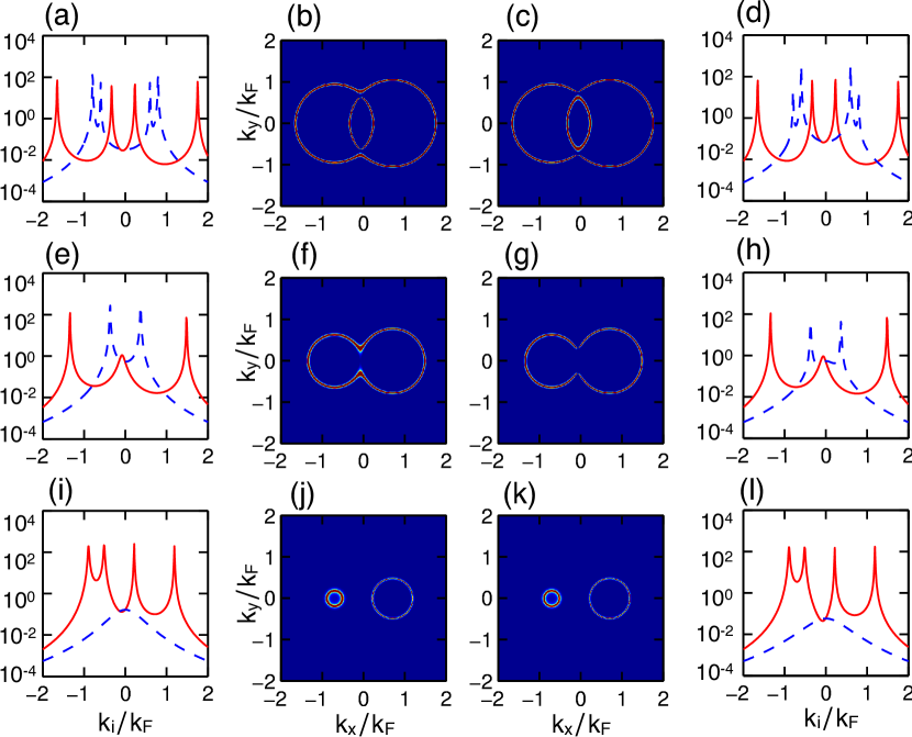
Figure 5: (color online) Finite temperature $(T/\epsilon_{F}=0.05)$ dimensionless spectral functions $2\pi\epsilon_{F}A_{s}({\bf k},\omega)$ at $\omega=\mu$ for ERD spin-orbit coupling $v/v_{F}=0.71$ and Zeeman fields $h_{y}/\epsilon_{F}=h_{z}/\epsilon_{F}=0.1$ In panels (a)-(d) $\mu/\epsilon_{F}=0.492$; (e)-(h) $\mu/\epsilon_{F}=0$; and (i)-(l) $\mu/\epsilon_{F}=-0.37$. The blue dashed lines are cuts along the direction $(k_{x}=0,k_{y},k_{z}=0)$ corresponding to $2\pi\epsilon_{F}A_{s}(k_{x}=0,k_{y},k_{z}=0,\omega=\mu)$, and the red solid lines are cuts along the direction $(k_{x},k_{y}=0,k_{z}=0)$ corresponding to $2\pi\epsilon_{F}A_{s}(k_{x},k_{y}=0,k_{z}=0,\omega=\mu)$. The two left-most columns describe the $A_{\uparrow}({\bf k})$ component, and the two right-most columns correspond to the $A_{\downarrow}({\bf k})$ component.

VI Momentum Distribution

To understand the momentum distribution for quantum degenerate Fermi gases in the presence of spin-orbit and crossed Zeeman fields, we look first at the expectation value $\langle{\hat{n}}_{\alpha}({\bf k})\rangle$ of the number operators ${\hat{n}}_{\alpha}({\bf k})=\Phi_{\alpha}^{\dagger}({\bf k})\Phi_{\alpha}({\bf k}),$ which describes the momentum distribution $n_{\alpha}({\bf k})$ in the helicity basis. In this case, the momentum distribution is $n_{\alpha}({\bf k})=n_{F}(\xi_{\alpha}({\bf k}))$, where $n_{F}(x)$ is the Fermi function.

The momentum distributions for the original spin states $s=(\uparrow,\downarrow)$ are defined as $n_{s}({\bf k})=\langle c_{{\bf k}s}^{\dagger}c_{{\bf k}s}\rangle.$ With the help of the unitary matrix ${\bf U}({\bf k})$ defined in Eq. (12), which relates the creation and annihilation operators in the helicity and the standard spin basis the momentum distributions become

$$n_{\uparrow}({\bf k})=u_{\bf k}^{2}n_{F}(\xi_{\Uparrow}({\bf k}))+|v_{\bf k}|^{2}n_{F}(\xi_{\Downarrow}({\bf k}))$$ (23)

for the up-spin $(\uparrow)$ component, and

$$n_{\downarrow}({\bf k})=|v_{\bf k}|^{2}n_{F}(\xi_{\Uparrow}({\bf k}))+u_{\bf k}^{2}n_{F}(\xi_{\Downarrow}({\bf k}))$$ (24)

for the down-spin $(\downarrow)$ component.

Such expressions can be also obtained from the general relation

$$n_{s}({\bf k})=\int_{-\infty}^{\infty}d\omega n_{F}(\omega)A_{s}({\bf k},\omega),$$ (25)

between the momentum distribution and the spectral function for fermions.

It is also convenient to obtain the momentum distribution sum $n_{+}({\bf k})=n_{\uparrow}({\bf k})+n_{\downarrow}({\bf k})$ and the momentum distribution difference $n_{-}({\bf k})=n_{\uparrow}({\bf k})-n_{\downarrow}({\bf k}).$ The first distribution can be written in terms of the Fermi functions only

$$n_{+}({\bf k})=n_{F}(\xi_{\Uparrow}({\bf k}))+n_{F}(\xi_{\Downarrow}({\bf k})),$$ (26)

while the second distribution can be written in terms of the Fermi functions and the components of the effective Zeeman field

$$n_{-}({\bf k})=\frac{h_{\parallel}}{|h_{{\rm eff}}({\bf k})|}\left[n_{F}(\xi_{\Uparrow}({\bf k})-n_{F}(\xi_{\Downarrow}({\bf k})\right].$$ (27)

In Fig. 6, we show momentum distributions $n_{s}({\bf k})$ at $T/\epsilon_{F}=0.05$ and in the regime where the Fermi system is largely degenerate, containing wide regions in momentum space where $n_{s}({\bf k})\approx 1$. The blue dashed lines represent cuts of $n_{s}({\bf k})$ along the ${\bf k}=(k_{x}=0,k_{y},k_{z}=0)$ direction, while the red solid lines represents cuts of $n_{s}({\bf k})$ along ${\bf k}=(k_{x},k_{y}=0,k_{z}=0)$. The left-most columns correspond to spin $\uparrow$, while the right-most columns represent spin $\downarrow$. For reference, we show in Figs. 6(a)-(d) the case with zero spin-orbit coupling and without Zeeman fields, corresponding to parameters $v/v_{F}=0$, $h_{y}/\epsilon_{F}=h_{z}/\epsilon_{F}=0$ chemical potential $\mu=1.0$. In this case, the momentum distributions for the two spin components are identical $n_{\uparrow}({\bf k})=n_{\downarrow}({\bf k})$, meaning that the populations are balanced with $n_{-}({\bf k})=0$, and induced polarization is $P_{\rm ind}=0$. In Figs. 6(e)-(h), we show momentum distributions for parameters $v/v_{F}=0.71$, $h_{y}/\epsilon_{F}=0$, $h_{z}/\epsilon_{F}=0.1$ and chemical potential $\mu=0.495$. Here, the momentum distributions acquire double plateaux structures along the direction ${\bf k}=(k_{x},k_{y}=0,k_{z}=0)$ due to the momentum shifts of the helicity bands as shown in Fig. 1(a). Additionally, the momentum distributions for different spin-components are no longer identical, such that $n_{\uparrow}({\bf k})\neq n_{\downarrow}({\bf k})$, or $n_{-}({\bf k})\neq 0$, and the induced polarization is non-zero taking the value $P_{\rm ind}=0.121$. In these two cases, parity is not violated and the momentum distributions are even functions of momentum under inversion symmetry. However, in Figs. 6(i)-(l), we show momentum distributions for parameters $v/v_{F}=0.71$, $h_{y}/\epsilon_{F}=h_{z}/\epsilon_{F}=0.1$, and chemical potential $\mu=0.492$, in which case the double plateaux structures are still preserved, population imbalance is present with $n_{-}({\bf k})\neq 0$ and induced polarization $P_{\rm ind}=0.120$. Most importantly parity is weakly violated since $n_{s}(-{\bf k})\neq n_{s}({\bf k})$.

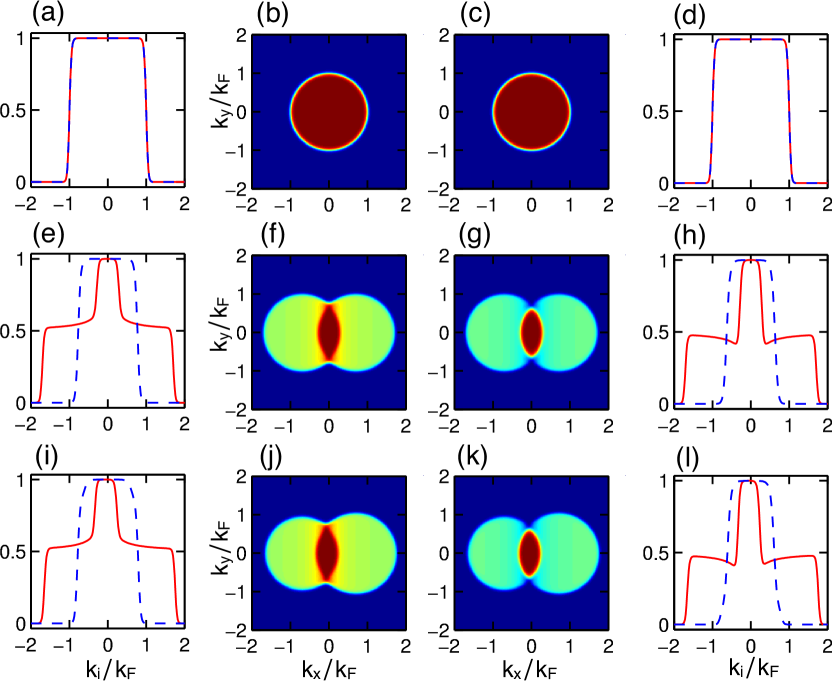
Figure 6: (color online) Finite temperature ($T/\epsilon_{F}=0.05$) momentum distributions $n_{\uparrow}({\bf k})$ (two left-most columns) and $n_{\downarrow}({\bf k})$ (two right-most columns). The parameters for (a)-(d) are ERD spin-orbit coupling $v/v_{F}=0$, Zeeman fields $h_{y}/\epsilon_{F}=h_{z}/\epsilon_{F}=0$, chemical potential $\mu/\epsilon_{F}=1.0$, and induced polarization $P_{\rm ind}=0$. Similarly, the parameters for (e)-(h) are $v/v_{F}=0.71$, $h_{y}/\epsilon=0$, $h_{z}/\epsilon_{F}=0.1$, $\mu/\epsilon_{F}=0.495$, and $P_{\rm ind}=0.121$; while for (i)-(l) the parameters are $v/v_{F}=0.71$, $h_{y}/\epsilon_{F}=h_{z}/\epsilon_{F}=0.1$, $\mu/\epsilon_{F}=0.492$, and $P_{\rm ind}=0.120$. The blue dashed lines represent cuts of $n_{s}({\bf k})$ along the ${\bf k}=(k_{x}=0,k_{y},k_{z}=0)$ direction, while the red solid lines represents cuts of $n_{s}({\bf k})$ along ${\bf k}=(k_{x},k_{y}=0,k_{z}=0)$.

In Fig. 7, we show momentum distributions $n_{s}({\bf k})$ at $T/\epsilon_{F}=0.05$ for parameters $v/v_{F}=0.71$, $h_{y}/\epsilon_{F}=h_{z}/\epsilon_{F}=0.1$, and varying chemical potentials $\mu/\epsilon_{F}$. We emphasize the regimes where parity is more strongly violated leading to momentum distributions without inversion symmetry: $n_{s}({-\bf k})\neq n_{s}({\bf k})$. The blue dashed lines represent cuts of $n_{s}({\bf k})$ along the ${\bf k}=(k_{x}=0,k_{y},k_{z}=0)$ direction, while the red solid lines represents cuts of $n_{s}({\bf k})$ along ${\bf k}=(k_{x},k_{y}=0,k_{z}=0)$. For reference, we show in Figs. 7(a)-(d) the case with $\mu/\epsilon_{F}=0.492$ and $P_{\rm ind}=0.120$, where the Fermi system is still largely degenerate, containing wide regions in momentum space with $n_{s}({\bf k})\approx 1$, and at the same time parity is violated only weakly. In Figs. 7(e)-(h), we show momentum distributions for $\mu/\epsilon_{F}=0$ and $P_{\rm ind}=0.143$, while in Figs. 7(i)-(l), we show momentum distributions for $\mu/\epsilon_{F}=-0.37$ and $P_{\rm ind}=0.105$. In both cases, the Fermi system is no longer degenerate, containing wide regions in momentum space where $n_{s}({\bf k})\ll 1$. In the last two cases the momentum distributions remain symmetric upon reflection along the $k_{y}$ or $k_{z}$ directions, but parity is more strongly violated leading to a highly asymmetric momentum distributions along the $k_{x}$ direction.

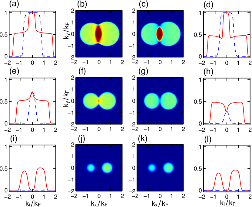
Figure 7: (color online) Finite temperature ($T/\epsilon_{F}=0.05$) momentum distributions $n_{\uparrow}({\bf k})$ (two left-most columns) and $n_{\downarrow}({\bf k})$ (two right-most columns). All panels corresponds to values of ERD spin-orbit coupling $v/v_{F}=0.71$, and Zeeman fields $h_{y}/\epsilon_{F}=h_{z}/\epsilon_{F}=0.1$. For (a)-(d) the chemical potential is $\mu/\epsilon_{F}=0.492$, and the induced polarization is $P_{\rm ind}=0.120$. Similarly, for (e)-(h) $\mu/\epsilon_{F}=0$, and $P_{\rm ind}=0.143$; while for (i)-(l) the parameters are $\mu/\epsilon_{F}=-0.37$, and $P_{\rm ind}=0.105$. The blue dashed lines represent cuts of $n_{s}({\bf k})$ along the direction ${\bf k}=(k_{x}=0,k_{y},k_{z}=0)$ direction, while the red solid lines represents cuts of $n_{s}({\bf k})$ along ${\bf k}=(k_{x},k_{y}=0,k_{z}=0)$.

Having discussed the momentum distribution at low temperatures, we analyze next the density of states of quantum degenerate fermions in the presence of spin-orbit coupling and crossed Zeeman fields.

VII Density of States

The density of states for spin $s$ can be written as

$$\rho_{s}(\omega)=\sum_{\bf k}A_{s}(\bf k,\omega),$$ (28)

in terms of the spectral function $A_{s}(\bf k,\omega).$ An analysis of the spin-dependent density of states is useful to provide the frequency (energy) dependence of the spin-polarization of the system.

In Fig. 8, we show the density of states $\rho_{s}(\omega)$ for various parameters with an energy broadening $\eta/\epsilon_{F}=0.01$. We show specifically the case of zero spin-orbit coupling and Zeeman fields in Fig. 8(a), which has the characteristic square-root frequency dependence for a three-dimensional system. In this case the system is not polarized and the tails below the bottom of the energy band are due to the finite energy broadening. We show two other situations for comparison corresponding to cases which are polarized with finite Zeeman fields, as well as with a finite spin-orbit coupling. In Fig. 8(b)-(c), we show that the band edges shift to lower frequencies when the Zeeman and spin-orbit fields are turned on. Furthermore, in Fig. 8(b) the spin-dependent density of states are shown for the case where parity is not violated, corresponding to $h_{y}/\epsilon_{F}=0$, $h_{z}/\epsilon_{F}=0.1$, and $v/v_{F}=0.71$; and in Fig. 8(c) the spin-dependent density of states are shown for the case where parity is violated, corresponding to $h_{y}/\epsilon_{F}=h_{y}/\epsilon_{F}=0.1$ and $v/v_{F}=0.71$. Since momentum is integrated over, there is no clear signature of parity violation in $\rho_{s}(\omega)$ as there is in momentum-resolved observables such as the spectral density $A_{s}({\bf k},\omega)$, momentum distribution $n_{s}({\bf k})$, or helicity dispersions $\epsilon_{\Uparrow}({\bf k})$ and $\epsilon_{\Downarrow}({\bf k})$ discussed earlier. However, we show the different spin-dependent density of states for comparison. The kinks present in these figures reflect the location of the maxima and minima of the helicity bands.

Having discussed the density of states, we present next an analysis of thermodynamic properties.

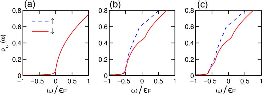
Figure 8: (color online) Spin-dependent density of states $\rho_{s}(\omega)$ in units of $N/\epsilon_{F}$ for (a) $v/v_{F}=0$ and $h_{z}/\epsilon_{F}=h_{y}/\epsilon_{F}=0$, (b) $v/v_{F}=0.71$ and $h_{y}/\epsilon_{F}=0$ and $h_{z}/\epsilon_{F}=0.1$, and (c) $v/v_{F}=0.71$ and $h_{z}/\epsilon_{F}=h_{y}/\epsilon_{F}=0.1$. The blue dashed line corresponds to $\rho_{\uparrow}({\omega})$ and the solid red line corresponds to $\rho_{\downarrow}({\omega})$.

VIII Thermodynamic Properties

From the energy spectrum of the Hamiltonian ${\bf H}_{0}$ defined in Eq. (10), we can obtain the partition function as

$$\mathcal{Z}={\rm Tr}\left[\exp(-{\bf H}_{0}/T)\right],$$ (29)

and the corresponding thermodynamic potential

$$\Omega=-T\ln\mathcal{Z}.$$ (30)

When no initial population imbalance is present, the total number of particles is fixed by

$$N=-\left(\frac{\partial\Omega}{\partial\mu}\right)_{T,V},$$ (31)

which determines the chemical potential $\mu$. In addition, because an external Zeeman field is present, we can define the induced polarization

$$P_{\rm ind}=\frac{N_{\uparrow}-N_{\downarrow}}{N_{\uparrow}+N_{\downarrow}},$$ (32)

where the number of particles in spin-state $s$ is

$$N_{s}=\sum_{\bf k}\int d\omega n_{F}(\omega)A_{s}({\bf k},\omega).$$ (33)

Next, we begin our analysis of thermodynamic variables that could be measured using the techniques already developed for ultra-cold fermions salomon-2010 ; zwierlein-2012a in the absence of spin-orbit coupling. In the discussion that follows, we will cover the pressure, the chemical potential, the isothermal compressibility and the induced magnetization (spin-polarization).

IX Pressure and Entropy

The pressure of ultra-cold fermions in the presence of spin-orbit coupling and crossed Zeeman fields is

$$P=-\frac{\Omega}{V}=-\frac{T}{V}\sum_{{\bf k},\alpha}\ln\left(1+e^{-\xi_{\alpha}({\bf k})/T}\right),$$ (34)

where $\Omega$ is thermodynamic potential, and $\alpha=(\Uparrow,\Downarrow)$ is the helicity spin index.

In Fig. 9, we show the scaled pressure $PV/(N\epsilon_{F})$ as a function of the Zeeman fields $h_{y}/\epsilon_{F}$ and $h_{z}/\epsilon_{F}$ for fixed spin-orbit coupling $v/v_{F}$. Notice that in the absence of spin-orbit and Zeeman fields the pressure reduces to the standard results of an non-interacting Fermi gas $PV/(N\epsilon_{F})=2/5$. The pressure is an even function of both $h_{y}$ and $h_{z}$ and is shown for a range of $h_{y}$ and $h_{z}$ varying from zero to $1.5\epsilon_{F}$. The spin-orbit coupling for Figs. 9(a)-(b) is $v/v_{F}=0$, and the pressure is completely isotropic in the $h_{y}$-$h_{z}$ plane, since the helicity bands $\epsilon_{\alpha}({\bf k})$ are also isotropic in $h_{y}$-$h_{z}$ plane and parity is preserved. However, in Fig. 9(c)-(d), where $v/v_{F}=0.71$, the pressure is anisotropic in the $h_{y}$-$h_{z}$ plane, since the helicity bands $\epsilon_{\alpha}({\bf k})$ are now anisotropic in the $h_{y}$-$h_{z}$ plane and are not invariant under parity.

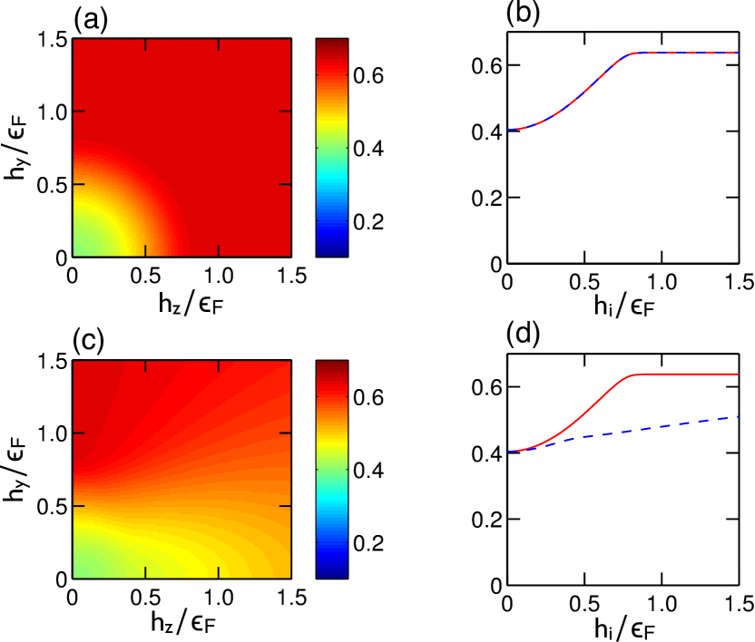
Figure 9: (color online) Pressure $PV/N\epsilon_{F}$ as a function of $h_{y}/\epsilon_{F}$ and $h_{z}/\epsilon_{F}$ at finite temperature ($T/\epsilon_{F}=0.05$) for (a)-(b) $v/v_{F}=0$ and (c)-(d) $v/v_{F}=0.71$. The red solid line represents $PV/N\epsilon_{F}$ as a function of $h_{y}/\epsilon_{F}$ at $h_{z}/\epsilon_{F}=0$, and the blue dashed line represents $PV/N\epsilon_{F}$ as a function of $h_{z}/\epsilon_{F}$ at $h_{y}/\epsilon_{F}=0$.

We note in passing that the entropy $S$ of the system can be easily extracted, by rewriting the thermodynamic potential as $\Omega=T\sum_{\bf k}\ln\left[1-n_{F}(\xi_{\alpha}({\bf k}))\right],$ when expressed in terms of the Fermi function $n_{F}(\xi_{\alpha}({\bf k}))$. Using the relation $S=-\left(\partial\Omega/\partial T\right)_{V,\mu},$ leads to the final result ($k_{B}=1$)

$$S=-\sum_{{\bf k}\alpha,m=\pm}\left\{n_{F}(m\xi_{\alpha}({\bf k}))\ln\left[n_{F}(m\xi_{\alpha}({\bf k}))\right]\right\},$$ (35)

which is nothing but the entropy of a non-interacting Fermi gas in the presence of spin-orbit coupling and crossed Zeeman fields. We will not show plots of the entropy, or of the specific heat, which can also be easily obtained, but rather discuss next the chemical potential and its dependence on the crossed Zeeman fields.

X Chemical Potential

The chemical potential $\mu$ in the Grand-canonical ensemble is determined by fixing the average number of particles given in Eq. (31), which can be rewritten as

$$N=\sum_{\bf k}n_{+}({\bf k}),$$ (36)

where $n_{+}({\bf k})$ is the total momentum distribution defined in Eq. (26). The behavior of $\mu$ as a function of the Zeeman fields $h_{y}$ and $h_{z}$ is shown in Fig. 10, which uses the fact that $\mu$ is an even function of these variables. The range of the Zeeman fields is also from $0$ to $1.5\epsilon_{F}$. The case where parity is preserved is shown if Fig. 10(a) and (b), corresponding to $v/v_{F}=0$, such that the chemical potential is isotropic in the $h_{y}$-$h_{z}$ plane. Similarly, in Fig. 10(c) and (d), we show the case corresponding to $v/v_{F}=0.71$, where parity is violated for any finite Zeeman component $h_{y}$. As a result the chemical potential $\mu/\epsilon_{F}$ is anisotropic in $h_{y}$-$h_{z}$ plane, because the helicity bands are neither even nor odd in momentum space. This demonstrates that the anisotropy of $\mu$ is a measure of parity violation. Another quantity that can be easily measured and that reveals a similar effect is the isothermal compressibility to be discussed next.

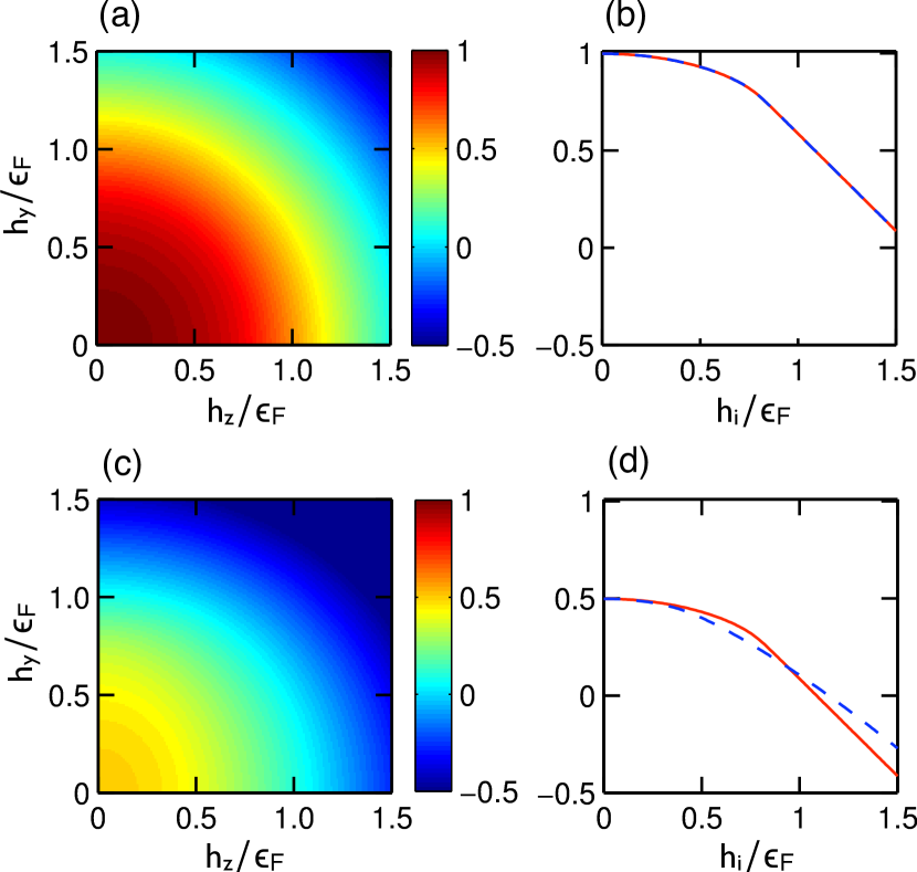
Figure 10: (color online) Finite temperature ($T/\epsilon_{F}=0.05$) chemical potential $\mu/\epsilon_{F}$ as a function of $h_{z}$ and $h_{y}$ is shown in (a)-(b) $v/v_{F}=0$ and in (c)-(d) for $v/v_{F}=0.71$. The red solid line represents $\mu(h_{y},h_{z}=0)/\epsilon_{F}$ and the blue dashed line represents $\mu(h_{y}=0,h_{z})/\epsilon_{F}$.

XI Isothermal Compressibility

The isothermal compressibility can be obtained from the knowledge of the pressure, as is defined as $\kappa_{T}=-(1/V)(\partial P/\partial V)_{T,N}.$ But in the Grand-canonical ensemble, where we need to fix the average number of particles, the isothermal compressibility can be directly written as

$$N^{2}\kappa_{T}=\left(\frac{\partial N}{\partial\mu}\right)_{T,V}.$$ (37)

Using the relation defined in Eq. (36) and noticing that the partial derivative $\left(\partial n_{F}(x)/\partial x\right)_{T,V}=-(1/T)n_{F}(x)n_{F}(-x),$ is directly related to the Fermi function $n_{F}(x)$, it is possible to write the expression for the isothermal compressibility as

$$N^{2}\kappa_{T}=\frac{1}{T}\sum_{{\bf k},\alpha}\left[n_{F}(\xi_{\alpha}({\bf k}))n_{F}(-\xi_{\alpha}({\bf k}))\right].$$ (38)

The experimental extraction of the isothermal compressibility from measurements of density fluctuations was suggested theoretically several years ago both in harmonically confined systems iskin-2005 and optical lattices iskin-2006 , and early improvements in the detection schemes of density fluctuations bloch-2005 ; bouchole-2006 ; steinhauer-2010 became sufficiently sensitive to extract this information from experimental data. In a recent experiment ketterle-2011 using laser speckles, the isothermal compressibility and the spin susceptibility were measured as a function of interaction parameter via the fluctuation dissipation theorem throughout the evolution from BCS to BEC superfluidity in balanced Fermi systems.

The atomic compressibility can be measured using the fluctuation-dissipation theorem relating the fluctuation in the density of particles $n=N/V$, where $N=\langle{\hat{N}}\rangle$ is the average number of particles, and ${\hat{N}}$ is particle-number operator. The relation between the isothermal compressibility $\kappa_{T}$ and particle-number (density) fluctuations is given by the relation:

$$\kappa_{T}=\frac{V}{T}\frac{\langle{\hat{N}}^{2}\rangle-\langle{\hat{N}}\rangle^{2}}{\langle{\hat{N}}\rangle^{2}}.$$ (39)

We see no major technical impediment to use techniques that are sensitive to spin-dependent density fluctuations in population imbalanced Fermi-Fermi mixtures with equal masses ketterle-2006 ; hulet-2006 , whether the imbalance is created initially via radio-frequency fields or via artificial spin-orbit and Zeeman fields. Such analysis was shown to be theoretically possible even for Fermi mixtures with unequal masses seo-2011a ; seo-2011b , and preliminary experimental results for these systems grimm-2010 ; grimm-2011 seem to indicate that indeed the compressibility and spin susceptibility matrix elements can be directly extracted from the local density and density fluctuation profiles.

Thus, we show in Fig. 11 the isothermal compressibility $\kappa_{T}$ as a function of both $h_{y}$ and $h_{z}$ for a range of $h_{y}$ and $h_{z}$ varying from zero to $1.5\epsilon_{F}$, at fixed temperature $(T=0.05\epsilon_{F})$. The spin-orbit coupling for Figs. 11(a)-(b) is $v/v_{F}=0$, and the compressibility is completely isotropic, as parity is preserved. However, in Fig. 11(c)-(d), where $v/v_{F}=0.71$, parity is broken for $h_{y}\neq 0$. This parity breaking is reflected in the helicity bands as discussed earlier, and manifests itself in the behavior of the compressibility versus $(h_{y},h_{z})$ via the anisotropy revealed in Fig. 11(c)-(d). Again such anisotropy is a reflection of the parity violation caused by the simultaneous presence of the ERD spin-orbit field and $h_{y}$. Another important property that can be measured is the spin polarization as a function of the Zeeman fields $h_{y},h_{z}$ for fixed spin-orbit coupling, which is discussed next.

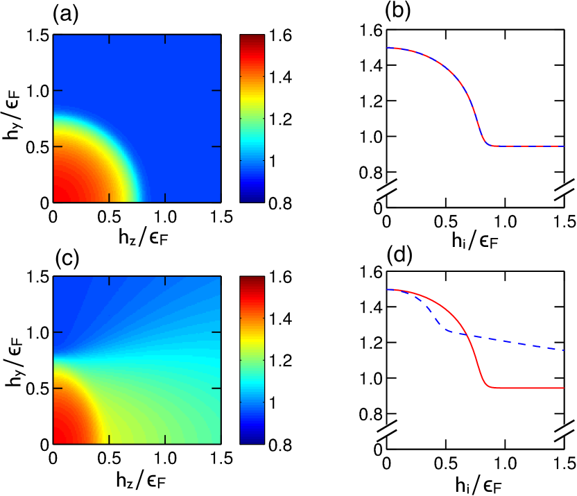
Figure 11: (color online) Finite temperature ($T/\epsilon_{F}=0.05$) isothermal compressibility $N^{2}\kappa_{T}$ in units of $N/\epsilon_{F}$ as a function of $h_{y}$ and $h_{z}$ is shown in (a)-(b) for $v/v_{F}=0$ and in (c)-(d) for $v/v_{F}=0.71$. The red solid line represents $N^{2}\kappa_{T}(h_{y},h_{z}=0)$ and the blue dashed line represents $N^{2}\kappa_{T}(h_{y}=0,h_{z})$.

XII Induced Spin Polarization

We can also analyze the induced spin polarization in the presence of crossed Zeeman fields and spin-orbit coupling. The spin polarization along the $i^{th}$ direction $(i=x,y,z)$ is given by the expectation value

$$\langle{\hat{S}}_{i}\rangle=\frac{1}{2}\sum_{\bf k}\langle\Psi^{\dagger}({\bf k}){\mathbf{\sigma}}_{i}\Psi({\bf k})\rangle.$$ (40)

Such general expression can be particularized for each component. For instance, the expectation value

$$\langle{\hat{S}}_{x}\rangle=\frac{1}{2}\sum_{\bf k}\left(\langle c_{{\bf k}\uparrow}^{\dagger}c_{{\bf k}\downarrow}\rangle+\langle c_{{\bf k}\downarrow}^{\dagger}c_{{\bf k}\uparrow}\rangle\right).$$ (41)

expressed in the original spin basis, can be rewritten in the helicity basis as

$$\langle{\hat{S}}_{x}\rangle=-\frac{1}{2}\sum_{\bf k}u_{\bf k}(v_{\bf k}+v_{\bf k}^{*})\left[n_{F}(\xi_{\Uparrow}({\bf k}))-n_{F}(\xi_{\Downarrow}({\bf k}))\right].$$ (42)

Analogously the expectation value of the spin-operator ${\hat{S}}_{y}$ in the original spin basis is

$$\langle{\hat{S}}_{y}\rangle=-\frac{i}{2}\sum_{\bf k}\left[\langle c_{{\bf k}\uparrow}^{\dagger}c_{{\bf k}\downarrow}\rangle-\langle c_{{\bf k}\downarrow}^{\dagger}c_{{\bf k}\uparrow}\rangle\right]$$ (43)

in the original spin basis can be written as

$$\langle{\hat{S}}_{y}\rangle=-\frac{i}{2}\sum_{\bf k}u_{\bf k}(v_{\bf k}-v_{\bf k}^{*})\left[n_{F}(\xi_{\Uparrow}({\bf k}))-n_{F}(\xi_{\Downarrow}({\bf k}))\right]$$ (44)

in the helicity basis. Lastly, the expectation value of ${\hat{S}}_{z}$ in the original spin basis is

$$\langle{\hat{S}}_{z}\rangle=\frac{1}{2}\sum_{\bf k}\left(\langle c_{{\bf k}\uparrow}^{\dagger}c_{{\bf k}\uparrow}\rangle-\langle c_{{\bf k}\downarrow}^{\dagger}c_{{\bf k}\downarrow}\rangle\right),$$ (45)

which can be rewritten in the helicity basis as

$$\langle{\hat{S}}_{z}\rangle=\frac{1}{2}\sum_{\bf k}(u_{\bf k}^{2}-|v_{\bf k}|^{2})\left[n_{F}(\xi_{\Uparrow}({\bf k}))-n_{F}(\xi_{\Downarrow}({\bf k}))\right].$$ (46)

Finally, the averages $\langle{\hat{S}}_{x}\rangle$ and $\langle{\hat{S}}_{y}\rangle$ can be expressed as real and imaginary parts of the transverse spin-polarization $\langle{\hat{S}}_{\perp}\rangle=\langle{\hat{S}}_{x}\rangle-i\langle{\hat{S}}_{y}\rangle,$ defined this way to be compatible with the definition of $h_{\perp}({\bf k})=h_{x}({\bf k})-ih_{y}({\bf k})$. The transverse spin-polarization takes the final form

$$\langle{\hat{S}}_{\perp}\rangle=\frac{1}{2}\sum_{\bf k}\frac{h_{\perp}({\bf k})}{\lvert h_{\rm eff}({\bf k})\rvert}\left[n_{F}(\xi_{\Uparrow}({\bf k}))-n_{F}(\xi_{\Downarrow}({\bf k}))\right].$$ (47)

Correspondingly the longitudinal spin polarization can be written as

$$\langle{\hat{S}}_{z}\rangle=\frac{1}{2}\sum_{\bf k}\frac{h_{\parallel}}{\lvert h_{\rm eff}({\bf k})\rvert}\left[n_{F}(\xi_{\Uparrow}({\bf k}))-n_{F}(\xi_{\Downarrow}({\bf k}))\right],$$ (48)

which is directly related to the induced population imbalance $P_{\rm ind}$ by the expression

$$P_{\rm ind}=\frac{2\langle{\hat{S}}_{z}\rangle}{N}$$ (49)

where $N=N_{\uparrow}+N_{\downarrow}$ is the total number of particles, as defined earlier.

For ERD spin-orbit coupling with field ${\bf h}_{ERD}=vk_{x}{\hat{\bf y}}$, the transverse field $h_{\perp}({\bf k})$ has only the y-component. This means that $\langle{\hat{S}}_{x}\rangle$ is identically zero for any value of $h_{y}$ and $h_{z}$ for any value of $v\neq 0$, given that $h_{x}({\bf k})=0$. However, $\langle{\hat{S}}_{y}\rangle$ is not identically zero for the ERD case above, unless parity is preserved in the helicity bands $\xi_{\alpha}({\bf k})$, which means $h_{y}=0$. For any finite value of $h_{y}$, $\langle{\hat{S}}_{y}\rangle$ is non-zero. This behavior is revealed in Fig. 12, where the expectation values $\langle{\hat{S}}_{y}\rangle$ and $\langle{\hat{S}}_{z}\rangle$ of spin polarization are shown as a function of $(h_{y}/\epsilon_{F},h_{z}/\epsilon_{F})$. In particular, we show in Fig. 12 the finite temperature ($T/\epsilon_{F}=0.05$) induced spin polarizations per particle $\langle S_{z}\rangle/N$ (two left-most columns) and $\langle S_{y}\rangle/N$ (two right-most columns) for ERD spin-orbit parameter $v/v_{F}=0$ from (a) through (d), and for $v/v_{F}=0.71$ from (e) through (h). In (a) and (e), the red solid line represents $\langle S_{z}\rangle/N$ as a function of $h_{y}/\epsilon_{F}$ at $h_{z}/\epsilon_{F}=0$, and the blue dashed line represents $\langle S_{z}\rangle/N$ as a function of $h_{z}\epsilon_{F}$ at $h_{y}/\epsilon_{F}=0$. In (d) and (h), the red solid line represents $\langle S_{y}\rangle/N$ as a function of $h_{y}/\epsilon_{F}$ at $h_{z}/\epsilon_{F}=0$, and the blue dashed line represents $\langle S_{y}\rangle/N$ as a function of $h_{z}/\epsilon_{F}$ at $h_{y}/\epsilon_{F}=0$.

Having analyzed several thermodynamic properties for non-interacting quantum degenerate ultra-cold fermions, which already present some fundamental non-trivial properties such as the violation of parity, we discuss next the effects of interactions and how parity violation affects the pairing temperature of such fermions and the superfluid order parameter.

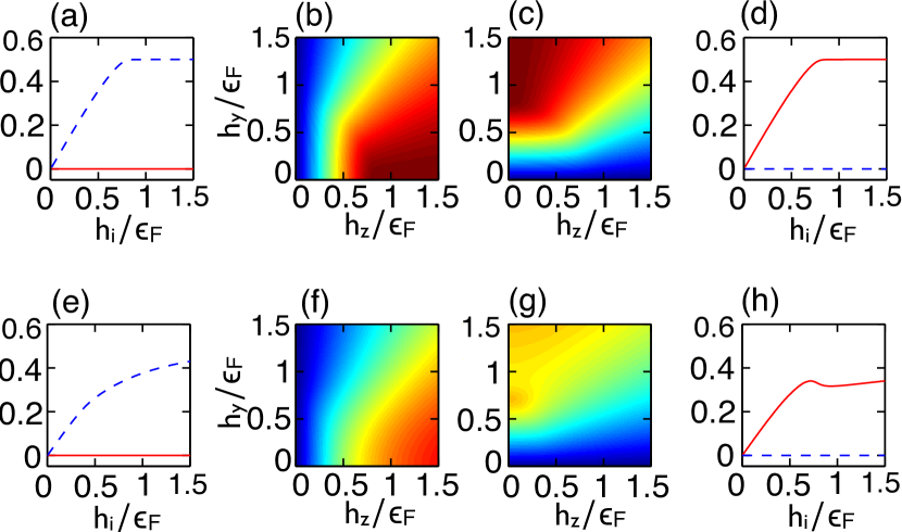
Figure 12: (color online) Finite temperature ($T/\epsilon_{F}=0.05$) induced spin polarizations per particle $\langle S_{z}\rangle/N$ (left two columns) and $\langle S_{y}\rangle/N$ (right two columns) are shown in (a)-(d) for $v/v_{F}=0$ and (e)-(h) for $v/v_{F}=0.71$. In (a) and (e), the red solid line represents $\langle S_{z}\rangle/N$ as a function of $h_{y}/\epsilon_{F}$ at $h_{z}/\epsilon_{F}=0$, and the blue dashed line represents $\langle S_{z}\rangle/N$ as a function of $h_{z}/\epsilon_{F}$ at $h_{y}/\epsilon=0$. In (d) and (h), the red solid line represents $\langle S_{y}\rangle/N$ as a function of $h_{y}/\epsilon_{F}$ at $h_{z}/\epsilon_{F}=0$, and the blue dashed line represents $\langle S_{y}\rangle/N$ as a function of $h_{z}/\epsilon_{F}$ at $h_{y}/\epsilon_{F}=0$.

XIII Effects of Interactions

In this section, we analyze briefly the effects of interactions in the presence of spin-orbit and crossed Zeeman fields, with focus on the dependence of the pairing temperature with respect to the interaction parameter for given spin-orbit and Zeeman fields. We also present a short discussion about the effects of parity violation on the superfluid order parameter.

The interaction Hamiltonian is

$${\cal H}_{I}=-g\int d{\bf r}\psi^{\dagger}_{\uparrow}({\bf r})\psi^{\dagger}_{\downarrow}({\bf r})\psi_{\downarrow}({\bf r})\psi_{\uparrow}({\bf r}),$$ (50)

where $g$ represents the strength of the contact interaction. Only $s$-wave scattering is considered in regards to the original spin states $\uparrow$ and $\downarrow$. Converting the interaction term into momentum space leads to

$${\cal H}_{I}=-g\sum_{\bf q}b^{\dagger}({\bf q})b({\bf q}),$$ (51)

where the pair creation operator with center of mass momentum ${\bf q}$ is $b^{\dagger}({\bf q})=\sum_{{\bf k}}\psi^{\dagger}_{\uparrow}({\bf k}+{\bf q}/2)\psi^{\dagger}_{\downarrow}(-{\bf k}+{\bf q}/2),$ and $g$ can be expressed in terms of the scattering length through the Lippman-Schwinger relation

$$\frac{V}{g}=-\frac{Vm}{4\pi a_{s}}+\sum_{\bf k}\frac{1}{2\epsilon_{\bf k}}.$$ (52)

The interaction Hamiltonian ${\cal H}_{I}$ can be written in the helicity basis as

$${\widetilde{\cal H}}_{I}=-g\sum_{{\bf q}\alpha\beta\gamma\delta}B^{\dagger}_{\alpha\beta}({\bf q})B_{\gamma\delta}({\bf q}),$$ (53)

where the indices $\alpha,\beta,\gamma,\delta$ cover $\Uparrow$ and $\Downarrow$ states. Pairing is now described by the operator

$$B_{\alpha\beta}({\bf q})=\sum_{\bf k}\Lambda_{\alpha\beta}({\bf k}_{1},{\bf k}_{2})\Phi_{\alpha}({\bf k}_{1})\Phi_{\beta}({\bf k}_{2})$$ (54)

and its Hermitian conjugate, with momentum indices ${\bf k}_{1}={\bf k}+{\bf q}/2$ and ${\bf k}_{2}=-{\bf k}+{\bf q}/2$. The matrix $\Lambda_{\alpha\beta}({\bf k}+{\bf q}/2,-{\bf k}+{\bf q}/2)$ is directly related to the matrix elements of the momentum dependent SU(2) rotation into the helicity basis, and reveals that the center of mass momentum ${\bf k}_{1}+{\bf k}_{2}={\bf q}$ and the relative momentum ${\bf k}_{1}-{\bf k}_{2}=2{\bf k}$ are coupled and no longer independent.

XIV Tensor Order Parameter

From Eq. (54) it is clear that pairing between fermions of momenta ${\bf k}_{1}$ and ${\bf k}_{2}$ can occur within the same helicity band (intra-helicity pairing) or between two different helicity bands (inter-helicity pairing). For pairing at ${\bf q}=0$, the order parameter for superfluidity is the tensor $\Delta_{\alpha\beta}({\bf k})=\Delta_{0}\Lambda_{\alpha\beta}({\bf k},-{\bf k}),$ where $\Delta_{0}=-g\sum_{\gamma\delta}\langle B_{\gamma\delta}({\bf 0})\rangle,$ leading to components:

$$\Delta_{\Uparrow\Uparrow}({\bf k})=\Delta_{0}\left(u_{\bf k}v_{-\bf k}-v_{\bf k}u_{-\bf k}\right)$$ (55)

for total helicity projection $\lambda=+1$;

$$\begin{array}[]{l}\Delta_{\Uparrow\Downarrow}({\bf k})=-\Delta_{0}\left(u_{\bf k}u_{-\bf k}+v_{\bf k}v_{-\bf k}^{*}\right)\\ \\ \Delta_{\Downarrow\Uparrow}({\bf k})=\Delta_{0}\left(u_{\bf k}u_{-\bf k}+v_{\bf k}^{*}v_{-\bf k}\right)\end{array}$$ (56)

for total helicity projection $\lambda=0$; and

$$\Delta_{\Downarrow\Downarrow}({\bf k})=\Delta_{0}\left(u_{\bf k}v_{-\bf k}^{*}-v_{\bf k}^{*}u_{-\bf k}\right)$$ (57)

for total helicity projection $\lambda=-1$.

It is very important to emphasize that for non-zero spin-orbit coupling and crossed Zeeman fields $h_{y}$ and $h_{z}$, the order parameter tensor $\Delta_{\alpha\beta}({\bf k})$ does not have well defined parity. For instance, while $\Delta_{\Uparrow\Uparrow}({\bf k})$ and $\Delta_{\Downarrow\Downarrow}({\bf k})$ have odd parity, the matrix elements $\Delta_{\Uparrow\Downarrow}({\bf k})$ and $\Delta_{\Downarrow\Uparrow}({\bf k})$ do not have well defined parity. However, we may still define singlet and triplet sectors for the helicity basis, such that the singlet sector $\Delta_{S,0}({\bf k})=\left[\Delta_{\Uparrow\Downarrow}({\bf k})-\Delta_{\Downarrow\Uparrow}({\bf k})\right]/2$ has even parity and the triplet sector defined by the components $\Delta_{\Uparrow\Uparrow}({\bf k})$, $\Delta_{T,0}({\bf k})=\left[\Delta_{\Uparrow\Downarrow}({\bf k})+\Delta_{\Downarrow\Uparrow}({\bf k})\right]/2$ and $\Delta_{\Downarrow\Downarrow}({\bf k})$ have odd parity for any value of the ERD spin-orbit coupling $v/v_{F}$ and crossed Zeeman fields $h_{y}/\epsilon_{F}$ and $h_{z}/\epsilon_{F}$. The preservation of parity in the singlet and triplet sectors is also true for the Rashba-only (RO) case, but the order parameter breaks time-reversal symmetry.

Within the mean field approximation, the Hamiltonian matrix in the helicity basis is

$${\widetilde{\bf H}}_{\rm MF}({\bf k})=\begin{pmatrix}\xi_{{\bf k}\Uparrow}&0&\Delta_{\Uparrow\Uparrow}({\bf k})&\Delta_{\Uparrow\Downarrow}({\bf k})\\ 0&\xi_{{\bf k}\Downarrow}&\Delta_{\Downarrow\Uparrow}({\bf k})&\Delta_{\Downarrow\Downarrow}({\bf k})\\ \Delta_{\Uparrow\Uparrow}^{*}({\bf k})&\Delta_{\Downarrow\Uparrow}^{*}({\bf k})&-\xi_{-{\bf k}\Uparrow}&0\\ \Delta_{\Uparrow\Downarrow}^{*}({\bf k})&\Delta_{\Downarrow\Downarrow}^{*}({\bf k})&0&-\xi_{-{\bf k}\Downarrow}\end{pmatrix}.$$ (58)

This Hamiltonian matrix is traceless, therefore the sum of its eigenvalues is zero, however the eigenvalues of $\widetilde{\bf H}_{\rm MF}({\bf k})$ are not invariant under parity. By labeling the eigenvalues as $E_{1}({\bf k})$, $E_{2}({\bf k})$, $E_{3}({\bf k})$ and $E_{4}({\bf k})$ in decreasing order of energy, and using the tracelessness condition then the sum $E_{3}({\bf k})+E_{4}({\bf k})=-\left[E_{1}({\bf k})+E_{2}({\bf k})\right]$ but each eigenvalue $E_{i}({\bf k})$ does not a well defined parity. Typically these eigenvalues are even in momentum space, but not here because the parity violation induced by the simultaneous presence of the crossed Zeeman fields and the spin-orbit coupling, thus, in the present case $E_{i}(-{\bf k})\neq E_{i}({\bf k})$. However a generalized particle-hole symmetry applies leading to $E_{2}({\bf k})=-E_{3}(-{\bf k})$ and $E_{1}({\bf k})=-E_{4}(-{\bf k}).$

The eigenvalues in this parity violating case can be obtained analytically for any mixture of Rashba and Dresselhaus terms from the determinant ${\rm Det}\left[\omega{\bf 1}-\widetilde{\bf H}_{\rm MF}({\bf k})\right],$ which leads to the characteristic quartic equation

$$\omega^{4}+a_{3}({\bf k})\omega^{3}+a_{2}({\bf k})\omega^{2}+a_{1}({\bf k})\omega+a_{0}({\bf k})=0$$ (59)

for each momentum ${\bf k}$. Here, the coefficient of the cubic term $a_{3}({\bf k})=-\sum_{i}E_{i}({\bf k})$ is the sum of the eigenvalues $E_{i}({\bf k})$ of the the Hamiltonian matrix $\widetilde{\bf H}_{\rm MF}({\bf k})$ and therefore vanishes. The coefficient of the quadratic term is $a_{2}({\bf k})=\sum_{i<j}E_{i}({\bf k})E_{j}({\bf k})$, while the coefficient of the linear term is $a_{1}({\bf k})=\sum_{i\neq j\neq\ell}E_{i}({\bf k})E_{j}({\bf k})E_{\ell}({\bf k}).$ The last coefficient is just the product of the four eigenvalues leading to $a_{0}=E_{1}({\bf k})E_{2}({\bf k})E_{3}({\bf k})E_{4}({\bf k})$.

In the particular case of ERD spin-orbit coupling with crossed Zeeman fields, the coefficients become $a_{3}=0$, and the coefficient of the quadratic term takes the form

$$a_{2}=-2\left({\widetilde{K}}_{+}^{2}({\bf k})+|\Delta_{0}|^{2}+|vk_{x}|^{2}+|h_{y}|^{2}+|h_{z}|^{2}\right),$$ (60)

while the coefficient of the linear term is

$$a_{1}=-8{\widetilde{K}}_{+}({\bf k})(vk_{x})h_{y},$$ (61)

and lastly the coefficient of the zero-th order term is

$$a_{0}=\xi_{\Uparrow}({\bf k})\xi_{\Downarrow}({\bf k})\xi_{\Uparrow}({-\bf k})\xi_{\Downarrow}(-{\bf k})+|\Delta_{0}|^{2}\alpha_{0}^{2}({\bf k})$$ (62)

where $\alpha_{0}^{2}({\bf k})=\left(2{\widetilde{K}}_{+}^{2}({\bf k})+|\Delta_{0}|^{2}+h_{0}^{2}({\bf k})\right)$ with $h_{0}^{2}({\bf k})=2|vk_{x}|^{2}-2|h_{y}|^{2}-2|h_{z}|^{2}.$ Here, ${\widetilde{K}}_{+}$ has the same definition used in the paragraph that follows Eq. (9), and is a measure of the kinetic energy with respect to the chemical potential.

Even in this simpler case of ERD spin-orbit coupling, the precise analytical form of the eigenvalues in the presence of crossed Zeeman fields is quite cumbersome, and we do not list them here explicitly. Rather, we discuss next the consequences of parity violation on the pairing temperature of ultra-cold fermions in the presence of spin-orbit and crossed Zeeman fields.

XV Pairing Temperature

From the excitation spectrum discussed above, we obtain the corresponding thermodynamic potential as

$$\Omega_{\rm MF}=V\frac{|\Delta_{0}|^{2}}{g}-\frac{T}{2}\sum_{{\bf k},j=1,4}\ln\left(1+e^{-E_{j}({\bf k})/T}\right)+\sum_{{\bf k}}\widetilde{K}_{+}({\bf k}),$$ (63)

from which the order parameter equation is determined via the minimization of $\Omega_{\rm MF}$ with respect to $|\Delta_{0}|^{2}$, leading to

$$\frac{V}{g}=-\frac{1}{2}\sum_{{\bf k},j}n_{F}\left(E_{j}({\bf k})\right)\frac{\partial E_{j}({\bf k})}{\partial|\Delta_{0}|^{2}},$$ (64)

where $n_{F}\left(E_{j}(\mathbf{k})\right)=1/(\exp\left(E_{j}({\bf k})/T\right)+1)$ is the Fermi function for energy $E_{j}({\bf k})$. The contact interaction $g$ can be elliminated in favor of the scattering length $a_{s}$ via the Lippman-Schwinger relation defined in Eq. (52).

The total number of particles $N=N_{\uparrow}+N_{\downarrow}$ is defined from the thermodynamic relation $N=-\left(\partial\Omega_{\rm MF}/\partial\mu\right)_{T,V},$ and leads to the corresponding number equation

$$N_{\rm MF}=\sum_{\bf k}\left[1-\frac{1}{2}\sum_{j}n_{F}\left(E_{j}({\bf k})\right)\frac{\partial E_{j}({\bf k})}{\partial\mu}\right],$$ (65)

since the system is assumed to have no initial population imbalance.

The self-consistent solutions of Eq. (64) and (65) guarantee the existence of mean field solutions for the order parameter amplitude $|\Delta_{0}|$ and the chemical potential $\mu$ as a function of the Zeeman fields $h_{y}$ and $h_{z}$, the spin-orbit coupling $v$ and scattering length $a_{s}$. However, the thermodynamic stability of the solutions obtained has to be tested against the maximum entropy condition (or minimum of the thermodynamic potential) over the same parameter space spanned by the variables $h_{y}$, $h_{z}$, $v$ and $a_{s}$, which determine the phase space of the present system. However, we discuss here only the effects of crossed Zeeman fields $h_{y}$, $h_{z}$ on the pairing temperature $T_{p}$ obtained by solving the mean-field self-consistent relations defined by Eq. (64) and Eq. (65) with the order parameter amplitude set to zero, i. e., $\Delta_{0}=0$.

In Fig. 13, we show the pairing temperature $T_{p}/\epsilon_{F}$ as a function of ERD spin-orbit coupling $v/v_{F}$ for selected values of $h_{y}$, $h_{z}$ and interaction parameter $1/(k_{F}a_{s})$. The lines are guides to the eye given that the number of points does not form a dense set. In (a) $h_{y}/\epsilon_{F}=0$ and in (b) $h_{y}/\epsilon_{F}=0.08$ both at $1/(k_{F}a_{s})=-0.5$, showing the behavior of $T_{p}$ on the BCS side of unitarity. In (c) $h_{y}/\epsilon_{F}=0$ and in (d) $h_{y}/\epsilon_{F}=0.4$ both at $1/(k_{F}a_{s})=1.0$, showing the behavior or $T_{p}$ on the BEC side of unitarity. In (a) and (b), the black-dotted line labels $h_{z}=0$, the red-dashed line $h_{z}/\epsilon_{F}=0.05$, the green-dash-dotted line $h_{z}/\epsilon_{F}=0.1$, and the blue-solid line $h_{z}/\epsilon_{F}=0.15$. However, in (c) and (d), the black-dotted line labels $h_{z}=0$, the red-dashed line $h_{z}/\epsilon_{F}=0.5$, the green-dash-dotted line $h_{z}/\epsilon_{F}=1$, and the blue-solid line $h_{z}/\epsilon_{F}=1.5$. Notice that the relative suppression of pairing with zero center of mass momentum in the BCS side $(1/(k_{F}a_{s})<0)$ is larger than in the BEC side $(1/(k_{F}a_{s})>0)$, since it relies strongly on pairing of states only close to the Fermi wavevectors ${\bf k}_{F}$ and $-{\bf k}_{F}$.

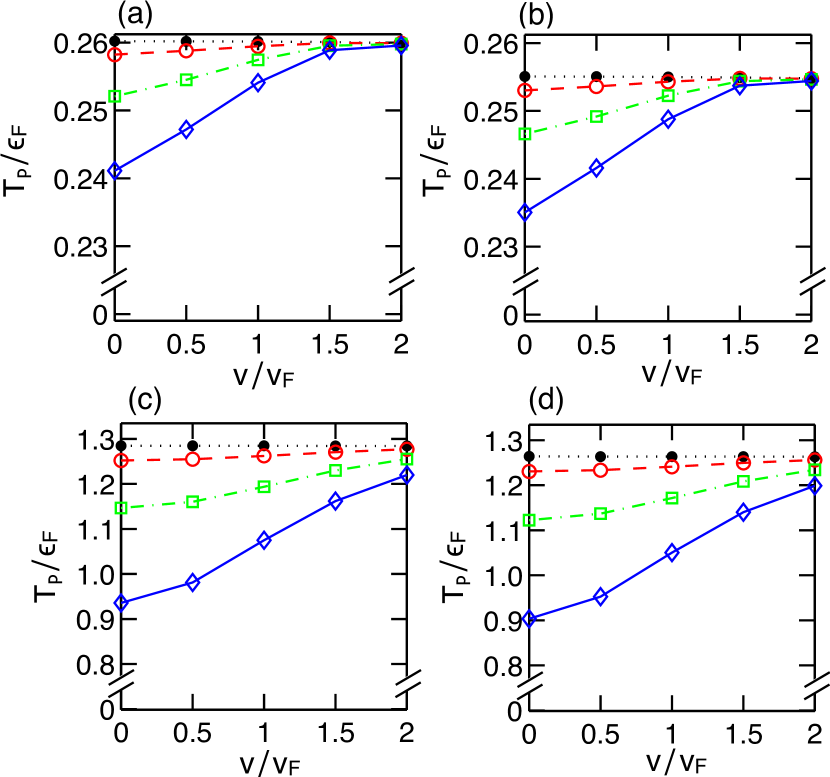
Figure 13: (color online) Pairing temperature $T_{p}/\epsilon_{F}$ as a function of ERD spin-orbit coupling $v/v_{F}$ for selected values of $h_{y}$, $h_{z}$ and interaction parameter $1/(k_{F}a_{s})$. In (a) $h_{y}/\epsilon_{F}=0$ and in (b) $h_{y}/\epsilon_{F}=0.08$ both for $1/k_{F}a_{s}=-0.5$. In (c) $h_{y}/\epsilon_{F}=0$ and in (d) $h_{y}/\epsilon_{F}=0.4$ both for $1/(k_{F}a_{s})=1.0$ For (a) and (b), the black dotted line labels $h_{z}=0$, the red dashed line $h_{z}/\epsilon_{F}=0.05$, the green dash-dotted line $h_{z}/\epsilon_{F}=0.1$, and the blue solid line $h_{z}/\epsilon_{F}=0.15$. In contrast, for (c) and (d), the black dotted line labels $h_{z}=0$, the red dashed line $h_{z}/\epsilon_{F}=0.5$, the green dash-dotted line $h_{z}/\epsilon_{F}=1$, and the blue solid line $h_{z}/\epsilon_{F}=1.5$. Notice that it is much easier to suppress pairing in the BCS side $(1/(k_{F}a_{s})<0)$, than in the BEC side $(1/(k_{F}a_{s})>0)$.

In Fig. 14, we show the pairing temperature $T_{p}/\epsilon_{F}$ versus scattering parameter $1/(k_{F}a_{s})$ for various values of the artificial Zeeman field components $h_{y}$ and $h_{z}$ and particular values of the ERD spin-orbit coupling $v$. The black cross line corresponds to parameters $v/v_{F}=0$, $h_{y}/\epsilon_{F}=h_{z}/\epsilon_{F}=0$, where there are no ERD spin-orbit coupling and no Zeeman fields. The red solid line corresponds to parameters $v/v_{F}=1$, $h_{y}/\epsilon_{F}=h_{z}/\epsilon_{F}=0$. Notice that these lines coincide, because the ERD spin-orbit field can be gauged away producing exactly the same results for any value of $v/v_{F}$ so long as $h_{y}/\epsilon_{F}=h_{z}/\epsilon_{F}=0$. The blue dashed-dotted line describes the case for parameters $v/v_{F}=1$, $h_{y}/\epsilon_{F}=0$, and $h_{z}/\epsilon_{F}=1$, showing that the presence of Zeeman field $h_{z}$ in the BCS regime produces an energy cost for pairing of Fermions with opposite momenta and zero center-of-mass momentum, thus reducing the pairing temperature substantially. However, the purple dashed line describing the situation corresponding to $v/v_{F}=1$, $h_{y}/\epsilon_{F}=0.4$, and $h_{z}/\epsilon_{F}=0$ shows a much stronger suppression of the pairing temperature than for the case of $v/v_{F}=1$, $h_{y}/\epsilon_{F}=0$, and $h_{z}/\epsilon_{F}=1$ (blue dot-dashed line), because it becomes much more difficult for fermions with opposite momenta to pair with zero center-mass-momentum due to the parity violation in the excitation spectrum of the fermions introduced by $h_{y}$ when $v/v_{F}\neq 0$. Lastly, the green dashed line shows the case of $v/v_{F}=1$, $h_{y}/\epsilon_{F}=0.4$, and $h_{z}/\epsilon_{F}=1$, where the combined effect of the Zeeman energy cost and parity violation lead to a dramatic reduction of the pairing temperature in the BCS region and even near unitarity.

Another important point to emphasize in Fig. 14 relates to the bending of $T_{p}$ in the two last cases corresponding to the dashed purple and dashed green lines. This bending indicate and instability of zero center-of-mass momentum pairing towards finite center-of-mass momentum pairing, and point of infinite slope in both curves indicates the separation of the two regimes. In the cases where the pairing temperature reflects the critical temperature of the system, the locations of infinite slope would correspond to a Lifshitz point, and a small region to the left of the negative slope regime would correspond to a superfluid with finite center of mass momentum, which is favored due to parity violation in the helicity bands.

For the parameters discussed the pairing temperature is not largely affected in the BEC regime, since the binding of fermions is controlled by the emergence of two-body bound states with binding energy $E_{b}$, and not by Cooper pairing in the presence of a Fermi sea. In the BEC regime, an estimate of $T_{p}$ can be given by considering the chemical equilibrium condition $\mu_{B}=2\mu_{F}$, where $\mu_{B}$ is the chemical potential of the bosons formed by tightly bound fermions, and $\mu_{F}$ is the chemical potential of unbound fermions. Since $T_{p}/\epsilon_{F}\gtrsim 1$, both bosons and unbound fermions are highly non-degenerate, and behave like classical ideal gases, in which case the chemical potential can be directly calculated and used to obtain the relation $T_{p}/\epsilon_{F}\sim|E_{b}/\epsilon_{F}|/\ln|E_{b}/\epsilon_{F}|^{3/2}$ to logarithmic accuracy. Here, the binding energy $E_{b}/\epsilon_{F}$ is a function of the interaction parameter $1/(k_{F}a_{s})$, the ERD spin-orbit parameter $v/v_{F}$ and the Zeeman fields $h_{y}/\epsilon_{F}$ and $h_{z}/\epsilon_{F}$. The logarithmic term is an entropy correction that reduces the pairing temperature $T_{p}$ to a value much lower than the absolute value of the binding energy $E_{b}$ of two fermions. The pairing temperature $T_{p}/\epsilon_{F}$ is essentially the same for values of $1/(k_{F}a_{s})>2$ (not shown in Fig. 12), because the binding energy $|E_{b}/\epsilon_{F}|\gg{\rm max}[v/v_{F},h_{y}/\epsilon_{F},h_{z}/\epsilon_{F}]$, in which case $|E_{b}/\epsilon_{F}|\approx 2/(k_{F}a_{s})^{2}$ and the pairing temperature is $T_{p}/\epsilon_{F}\sim[2/(k_{F}a_{s})^{2}]/\ln[1/(k_{F}a_{s})]^{3}$, which agrees with the numerical calculations in the regime of $1/(k_{F}a_{s})\gg 1$.

We will not present here a discussion of the condensation or critical temperature $T_{c}$ as it requires a full calculation of fluctuations effects, which is now underway han-seo-sdm-2012 . However, in the extreme BEC regime, where $1/(k_{F}a_{s})\gg 1$, the critical temperature $T_{c}$ can be obtained from the Bose-Einstein condensation temperature $T_{c}\approx T_{BEC}=[n_{B}/\zeta(3/2)]^{2/3}2\pi/m_{B}$, where the zeta function $\zeta(3/2)\approx 2.6124$, the density of bosons $n_{B}=n/2$ is half the density $n$ of fermions, and $m_{B}$ is the mass of bosons which is a function of the mass $m$ of fermions, and the parameters $v$, $h_{y}$ and $h_{z}$. The ratio $m_{B}/m$ can be parameterized by the dimensionless ratios $v/v_{F}$, $h_{y}/\epsilon_{F}$ and $h_{z}/\epsilon_{F}$. In the limit of $1/(k_{F}a_{s})\to\infty$ with finite $v/v_{F}$, $h_{y}/\epsilon_{F}$ and $h_{z}/\epsilon_{F}$, the Boson mass $m_{B}\to 2m$, but corrections depending on the aforementioned ratios tend to make the mass heavier, and for finite but large $1/(k_{F}a_{s})$ this mass increase tends to reduce $T_{BEC}$. However, the effect of interactions between the effective bosons is very subtle and the understanding of its dependence on the dimensionless ratios $1/(k_{F}a_{s})$, $v/v_{F}$, $h_{y}/\epsilon_{F}$, and $h_{z}/\epsilon_{F}$ is being currently investigated han-seo-sdm-2012 .

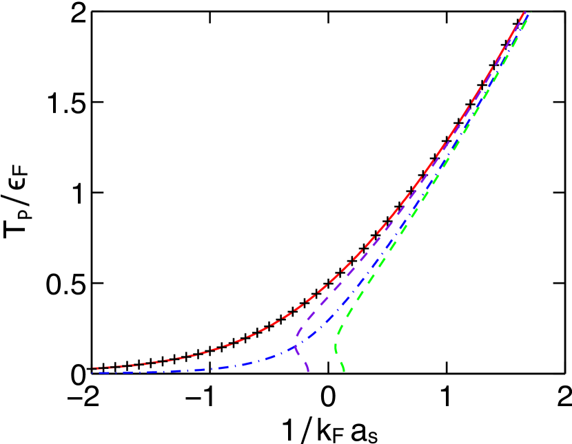
Figure 14: (color online) The plot of the pairing temperature $T_{p}/\epsilon_{F}$ as a function of $1/k_{F}a_{s}$. The black dotted line represent the case for ERD spin-orbit coupling $v/v_{F}=0$, and Zeeman fields $h_{y}/\epsilon_{F}=h_{z}/\epsilon_{F}=0$; the red solid line for corresponds to $v/v_{F}=1$, $h_{y}/\epsilon_{F}=0$, and $h_{z}/\epsilon_{F}=0$; the blue dashed-dotted line to $v/v_{F}=1$, $h_{y}/\epsilon_{F}=0$, and $h_{z}/\epsilon_{F}=1$; the purple dashed line describes the case of $v/v_{F}=1$, $h_{y}/\epsilon_{F}=0.4$, and $h_{z}=0$; and finally the green dashed line corresponds to $v/v_{F}=1$, $h_{y}/\epsilon_{F}=0.4$, and $h_{z}/\epsilon_{F}=1$.

After a detailed discussion of the effects of parity violation on interactions, order parameter, and pairing temperature $T_{p}$, which is is dramatically affected in the BCS regime, but largely unaffected in the BEC regime for the parameter range investigated, we are ready to present our conclusions.

XVI Conclusions

We have analyzed the normal state of a degenerate Fermi gas in the presence of artificial spin-orbit coupling and crossed Zeeman fields. The specific form of the spin-orbit field chosen corresponds to a mixture of equal Rashba and Dresselhaus (ERD) terms ${\bf h}_{ERD}({\bf k})=vk_{x}\hat{\bf y}$, which has been experimentally realized. The artificial Zeeman field $h_{z}$ along a defined spin quantization $z$ corresponds to the Raman intensity of the laser beams, and the crossed Zeeman field $h_{y}$ pointing along the same direction the ERD spin-orbit field corresponds to the frequency detuning from the atomic transition coupling two spin states.

In such configuration, the eigenvalues of the non-interacting problem are obtained in a generalized helicity basis, where the helicity spin projection points either along or opposite to the quantization axis defined by the effective magnetic field ${\bf h}_{\rm eff}({\bf k})=(0,h_{y}+vk_{x},h_{z}).$ In this case, we have shown that the presence of spin-orbit and crossed Zeeman fields lead to parity violation in the excitation spectrum of the non-interacting Fermi gas, which has immediate consequences for the Fermi surface, spectral density and momentum distribution, which also do not have well defined parity. Such parity violation emerges in momentum-resolved spectroscopic quantities because they are all functions of the magnitude $|{\bf h}_{\rm eff}({\bf k})|$ of the effective field ${\bf h}_{\rm eff}({\bf k})=(0,h_{y}+vk_{x},h_{z})$, which does not have well defined parity, since ${\bf h}_{\rm eff}(-{\bf k})=(0,h_{y}-vk_{x},h_{z})$.

In addition, we have shown that information on parity violation can be extracted from momentum-averaged thermodynamic properties such as pressure, entropy, chemical potential, compressibility, and spin-polarization as a function of crossed Zeeman field components $h_{y}/\epsilon_{F}$ and $h_{z}/\epsilon_{F}$ for fixed spin-orbit coupling $v/v_{F}$ at fixed temperature $T$. A signature of parity violation is the different behavior of any chosen thermodynamic quantity as a function of $h_{y}$ for $h_{z}=0$ and as a function of $h_{z}$ for $h_{y}=0$. This anisotropy of thermodynamic properties in the $(h_{y},h_{z})$ plane for finite spin-orbit coupling $v/v_{F}$ is a direct reflection of the lack of parity (inversion symmetry).

Lastly, we analyzed the effects of interactions for a degenerate Fermi gas when parity is broken, and investigated how parity violation influences the order parameter of a uniform superfluid and the fermion pairing temperature. We noticed that the order parameter tensor for a uniform superfluid in the generalized helicity basis no longer possesses inversion symmetry, however singlet and triplet pairing in can still be defined this basis and preserves parity. Furthermore, we found that the effects of parity violation are strong in the pairing temperature of fermions, because it becomes increasingly more difficult to pair states with zero center of mass momentum between helicity bands with progressively larger loss of inversion symmetry.

References

(1)
J. P. Gaebler, J. T. Stewart, J. L. Bohn, and D. S. Jin
Phys. Rev. Lett. 98, 200403 (2007).
(2)
Yasuhisa Inada, Munekazu Horikoshi, Shuta Nakajima, Makoto Kuwat-Gonokami,
Masahito Ueda, and Takashi Mukaiyama,
Phys. Rev. Lett. 101, 100401 (2008).
(3)
J. Fuchs, C. Ticknor, P. Dyke, G. Veeravalli, E. Kuhnle, W. Rowlands,
P. Hannaford, and C. J. Vale,
Phys. Rev. A 77, 053616 (2008).
(4)
R. A. W. Maier, C. Marzok, C. Zimmermann,
and Ph. W. Courteille,
Phys. Rev. A 81, 064701 (2010).
(5)
N. Navon, S. Nascimbène, F. Chevy, and C. Salomon,
Science 328, 729, (2010),
(6)
Mark J. H. Ku, Ariel T. Sommer, Lawrence W. Cheuk, Martin W. Zwierlein
Science 335, 563 (2012).
(7)
C.-H. Cheng and S.-K. Yip,
Phys. Rev. B 75, 014526 (2007).
(8)
T.-L. Ho and Q. Zhou,
Nature Phys. 6, 131 (2010).
(9)
E. I. Rashba,
Sov. Phys. Solid State 2, 1109 (1960).
(10)
G. Dresselhaus,
Phys. Rev. 100, 580 (1955).
(11)
Y. J. Lin, K. Jimenez-Garcia, and I. B. Spielman,
Nature 471, 83 (2011).
(12)
M. Chapman and C. Sá de Melo, Nature 471, 41 (2011).
(13)
Jayantha P. Vyasanakere, Shizhong Zhang, and Vijay B. Shenoy,
Phys. Rev. B 84, 014512 (2011).
(14)
Ming Gong, Sumanta Tewari, and Chuanwei Zhang,
Phys. Rev. Lett. 107, 195303 (2011).
(15)
Zeng-Qiang Yu, and Hui Zhai,
Phys. Rev. Lett. 107, 195305 (2011).
(16)
Hui Hu, Lei Jiang, Xia-Ji Liu, and Han Pu,
Phys. Rev. Lett. 107, 195304 (2011).
(17)
M. Iskin and A. L. Subasi,
Phys. Rev. Lett. 107, 050402 (2011).
(18)
L. P. Gorkov and E. I. Rashba,
Phys. Rev. Lett. 87, 037004 (2001).
(19)
S. K. Yip,
Phys. Rev. B 65, 144508 (2002).
(20)
P. Frigeri, D.F. Agterberg, A. Koga1, and M. Sigrist,
Phys. Rev. Lett. 92, 097001 (2004).
(21)
C. Zhang, S. Tewari, R. M. Lutchyn, and S. Das Sarma,
Phys. Rev. Lett. 101, 160401 (2008).
(22)
X.-J. Liu, M. F. Borunda, X. Liu, and J. Sinova,
Phys. Rev. Lett. 102, 046402 (2009).
(23)
Li Han, C. A. R. Sá de Melo,
Phys. Rev. A 85, 011606(R) (2012).
(24)
Kangjun Seo, Li Han, C. A. R. Sá de Melo,
Phys. Rev. A 85, 033601 (2012).
(25)
Kangjun Seo, Li Han and C. A. R. Sá de Melo,
arXiv:1110.6364v1 (2011).
(26)
Kangjun Seo, Li Han, C. A. R. Sá de Melo,
Phys. Rev. Lett. 109, 105303 (2012).