Intrinsic Dynamical Fluctuation Assisted Symmetry Breaking in Adiabatic Following

Abstract

Classical adiabatic invariants in actual adiabatic processes possess intrinsic dynamical fluctuations. The magnitude of such intrinsic fluctuations is often thought to be negligible. This widely believed physical picture is contested here. For adiabatic following of a moving stable fixed-point solution facing a pitchfork bifurcation, we show that intrinsic dynamical fluctuations in an adiabatic process can assist in a deterministic and robust selection between two symmetry-connected fixed-point solutions, irrespective of the rate of change of adiabatic parameters. Using a classical model Hamiltonian also relevant to a two-mode quantum system, we further demonstrate the formation of an adiabatic hysteresis loop in purely Hamiltonian mechanics and the generation of a Berry phase via changing one single-valued parameter only.

Introduction – Adiabatic theorem is about the dynamical behavior of a Hamiltonian system whose parameters are changing slowly with time. It constitutes a fundamental topic in Hamiltonian mechanics adiabatic . For example, Einstein was among the first to recognize the importance of classical adiabatic invariants in understanding quantization Gutzwiller . In recent years, there are still considerable interests in several aspects of adiabatic theorem in both quantum mechanics quantitativecondition and classical mechanics ZhangAOP2012 .

Figure 1: A supercritical pitchfork bifurcation in a classical Hamiltonian system parameterized by $R$. The solid (dashed) lines represent the phase space locations of stable (unstable) fixed points as a function of $R$. (a) When $R$ exceeds $R_{1}$, a stable fixed point splits into two stable and one unstable fixed points. One then wonders which branch the system will land on as $R$ adiabatically increases beyond $R_{1}$. (b) The bifurcated fixed points merge back when $R$ exceeds $R_{2}$. If $R$ first increases from $R<R_{1}$ to $R>R_{2}$ and later returns to $R<R_{1}$, then an adiabatic hysteresis loop may be formed.

Classical adiabatic following is the subject of this study, but our findings are also relevant to certain quantum systems. We start from the fact that classical adiabatic theorem is not an exact theorem: an actual adiabatically evolving trajectory fluctuates around an idealized solution predicted by the adiabatic theorem. Adiabatic invariants hence possess intrinsic dynamical fluctuations (IDF’s) ZhangAOP2012 ; Berry1996 ; adam ; mag ; liu . The magnitude of such fluctuations, typically proportional to the rate of change of adiabatic parameters, becomes extremely small in truly slow adiabatic processes. So except for special quantities that can accumulate IDF during an adiabatic process liu ; ZhangAOP2012 (e.g., in calculations of dynamical angles), IDF does not seem to be interesting or physically relevant. As shown in this Letter via both theory and computational examples, this perception is about to change.

Bifurcation phenomenon is ubiquitous in nonlinear systems and it is of fundamental interest to many topics in physics, among which we mention localization-delocalization phase transitions and symmetry breaking wubiao ; wubiao2 ; luis ; leech ; ZhangPRA2008 ; liu2 . Here we consider the adiabatic following of a stable fixed-point solution, which, as a result of a varying adiabatic parameter, moves towards a supercritical pitchfork bifurcation. As schematically shown in Fig. 1(a), two new stable fixed points and one unstable fixed point emerge after the adiabatic parameter (denoted $R$) slowly passes the bifurcation point at $R=R_{1}$. It is then curious to know among the three fixed points, which fixed-point solution the system will land on and whether the selection is predictable. It is found, both theoretically and numerically, that IDF is crucial for a deterministic and robust selection between the symmetry-connected pair of stable fixed-point solutions, regardless of how slow the adiabatic process is. As such, through crossing the bifurcation point, a tiny IDF is amplified to a macroscopic level after the bifurcation: it determines the fate of the trajectory afterwards by “forcing” the system to make a selection between symmetry-breaking solutions. We term this as deterministic symmetry breaking, because there is no need for external noise to initiate the symmetry-breaking. The selection process is robust because, unlike symmetry-breaking selection processes studied previously liu2 , it is independent of the dynamical details. Figure 1(b) depicts an interesting situation that involves a second bifurcation at $R=R_{2}$, after which the three fixed-point solutions merge back to one stable fixed point. We shall show that this case may allows us to generate a Berry phase by manipulating one single-valued parameter only.

Preliminaries – We recently developed a general description of IDF in classically integrable systems ZhangAOP2012 , which can be reduced to a rather simple form for stable fixed-point solutions in phase space. In particular, let us consider a one-dimensional Hamiltonian $H(q,p;R)$, with $(q,p)$ being the canonical variables, $R$ a system parameter to be tuned slowly, and its stable fixed point solutions denoted by $[\bar{q}(R),\bar{p}(R)]$. According to the traditional picture offered by classical adiabatic theorem, a stable phase space fixed point has zero action, so when $R$ varies slowly, the system must retain its zero action as an adiabatic invariant and therefore must follow the instantaneous fixed point $[\bar{q}(R),\bar{p}(R)]$. This is however a picture without IDF. The actual time evolving state $(q,p)$ deviates from $[\bar{q}(R),\bar{p}(R)]$,

$$q=\bar{q}+\delta q,\ \ p=\bar{p}+\delta p.$$ (1)

where $(\delta q,\delta p)$ are IDF on top of the idealized adiabatic solution $[\bar{q}(R),\bar{p}(R)]$ with $R=R(t)$. It is straightforward to see why $(\delta q,\delta p)$ has to be nonzero: were it indeed zero, then by definition of a fixed point, we have $\frac{\partial H(q,p,R)}{\partial q}=\frac{\partial H(q,p,R)}{\partial p}=0$, indicating that the current state $(q,p)$ cannot evolve and hence the system can never do adiabatic following with a moving fixed-point solution. This indicates that nonzero $(\delta q,\delta p)$ is not due to nonadiabaticity. Rather, it is intrinsic and must exist for adiabatic following to occur. Our theory applied to this case ZhangAOP2012 gives (see also liu )

$$\left(\begin{array}[]{c}\langle\delta{p}\rangle\\ \langle\delta{q}\rangle\end{array}\right)={\Gamma}^{-1}\left(\begin{array}[]{c}\frac{\partial\bar{p}}{\partial R}\\ \frac{\partial\bar{q}}{\partial R}\end{array}\right)\cdot\frac{dR}{dt},$$ (2)

where

$$\Gamma=\left(\begin{array}[]{cc}-\frac{\partial^{2}H}{\partial q\partial p}&-\frac{\partial^{2}H}{\partial q\partial q}\\ \frac{\partial^{2}H}{\partial p\partial p}&\frac{\partial^{2}H}{\partial p\partial q}\end{array}\right)_{p=\bar{p},q=\bar{q}},$$ (3)

and $\langle\cdot\rangle$ denotes an average over all possible initial conditions of $(\delta q,\delta p)$. As seen from Eq. (2), so long as $\Gamma^{-1}$ exists, then the scale of IDF is proportional to $\frac{dR}{dt}\equiv V$, the speed of adiabatic manipulation. The magnitude of $(\delta q,\delta p)$ is then deceptively small (for a sufficiently small $V$), but nonzero in general.

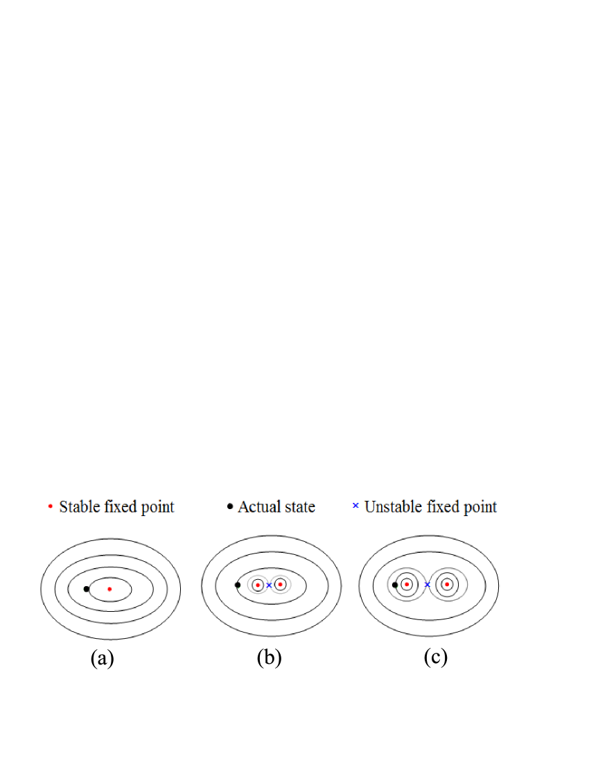
Figure 2: (color online) Impact of intrinsic dynamical fluctuations on the crossing of a pitchfork bifurcation. (a) The system’s actual state is on the left of the instantaneous fixed point. (b) Immediately after the bifurcation, the actual state is still shifted to the left of all the fixed points. (c) As two stable fixed points split further, the actual state gets trapped by, and starts to adiabatically follow, the stable fixed-point solution on the left.

We now examine how nonzero $(\delta q,\delta p)$ impacts the adiabatic following of $[\bar{q}(R),\bar{p}(R)]$ that eventually undergoes a supercritical pitchfork bifurcation at $R=R_{1}$. First, right before the adiabatic parameter $R$ reaches the bifurcation point $R_{1}$, the system’s actual state $(q,p)$ must deviate from the instantaneous solutions $[\bar{q}(R),\bar{p}(R)]$ by $(\delta q,\delta p)$. Without loss of generality and based on Eq. (2), the actual time-evolving state $(q,p)$ is assumed to be slightly shifted to the left side of the instantaneous fixed point $[\bar{q}(R),\bar{p}(R)]$. This is illustrated in Fig. 2(a), where the periodic orbits (associated with a fixed $R$) around $[\bar{q}(R),\bar{p}(R)]$ are also shown. The second stage is illustrated by Fig. 2(b), where $R$ only slightly exceeds $R_{1}$. There the bifurcation already occurs but the actual state does not “feel” the bifurcation yet: it continues to stay on the left side of all the three new fixed points. So the actual left-shifted state is located on an orbit (if $R$ were fixed) surrounding all the fixed points (this is confirmed in our numerical studies). The line shown in Fig. 2(b) passing through the unstable fixed point represents the separatrix. In the last stage, $R$ further increases, the two stable fixed points split further, with the stable fixed point moving to the left capturing the actual state [see Fig. 2(c)]. During the ensuing adiabatic following, the actual state then adiabatically follows the instantaneous fixed point on the left. Clearly then, if, as $R$ approaches a bifurcation point, IDF can induce a definite shift (to the left or the right) of the actual state with respect to $[\bar{q}(R),\bar{p}(R)]$, then the system will be trapped, deterministically, by one of the two stable fixed-point solutions after the bifurcation. Note that, exactly because of IDF, the actual state always stays away from the vicinity of the unstable fixed point (the extremely slow part of a separatrix). As a result the diverging time scale associated with the whole separatrix does not affect adiabatic following here. This understanding will be confirmed in our following numerical experiments.

Model Hamiltonian – Here we turn to a concrete Hamiltonian system with supercritical pitchfork bifurcations. Specifically, we choose

$$H=-\frac{c}{2}q^{2}-R\sqrt{1-q^{2}}\cos(p)+\Delta\sqrt{1-q^{2}}\sin(p)$$ (4)

in dimensionless units, with $c>\Delta>0$. Interestingly, this system has two bifurcation points at $R_{1}=-\sqrt{c^{2}-{\Delta^{2}}}$ and $R_{2}=\sqrt{c^{2}-\Delta^{2}}$. Define $\eta=\sqrt{1-(R^{2}+\Delta^{2})/c^{2}}$ and $\mu=\arctan(-\Delta/R)$. In the negative regime of $R$, the stable fixed point is $(\bar{q},\bar{p})=(0,\mu-\pi)$ for $R<R_{1}$, which then bifurcates into two stable fixed points at $(\mp\eta,\mu-\pi)$. In the positive regime of $R$, the two stable fixed points are at $(\mp\eta,\mu)$ for $R<R_{2}$ and then merge back to one stable fixed point at $(0,\mu)$. Note that this model Hamiltonian is invariant under the joint operation of space reflection ($\mathcal{P}$) $q\rightarrow-q$ and time reversal ($\mathcal{T}$) $t\rightarrow-t$. Therefore, for cases with only one stable fixed point, the solution itself has the same $\mathcal{P}$$\mathcal{T}$ symmetry, and for cases with two stable fixed points, the pair are transformed to each other under the $\mathcal{P}$$\mathcal{T}$ operations, with each individual fixed point being a symmetry-breaking solution. The phase space locations of these stable fixed-point solutions for various fixed values of $R$ are shown by the solid lines in Fig. 3.

Another motivation to choose $H$ in Eq. (4) is that it describes a two-mode many-body quantum system on the mean-field level. Consider the following mean-field Hamiltonian in dimensionless units ($\hbar=1$),

$$\hat{H}_{\text{m}}=\left(\begin{array}[]{cc}c(|b|^{2}-|a|^{2})&-R-i\Delta\\ -R+i\Delta&-c(|b|^{2}-|a|^{2})\end{array}\right),$$ (5)

where $a$ and $b$ are quantum amplitudes on two modes, $c$ represents the self-interaction strength, and $R\pm i\Delta$ represents inter-mode coupling. By rewriting $a=|a|e^{i\phi_{a}}$, $b=|b|e^{i\phi_{b}}$, $p=\phi_{b}-\phi_{a}$, and $q=|b|^{2}-|a|^{2}$, the time evolution of $q$ and $p$, as obtained from the Schrödinger equation for this quantum model, becomes precisely that under the classical model Hamiltonian $H$ in Eq. (4). The fixed points of $H$ become eigenstates of $\hat{H}_{\text{m}}$; the adiabatic following when crossing a bifurcation for $H$ is mapped to the issue of adiabatic following as degenerate eigenstates of $\hat{H}_{\text{m}}$ emerge. One possible realization of $\hat{H}_{\text{m}}$ is a Bose-Einstein condensate (BEC) in a double-well potential, with the imaginary coupling constant $\Delta$ implemented via phase imprinting on one well Denschlag . $\hat{H}_{\text{m}}$ may also be realized in nonlinear optics by using two nonlinear optical waveguides with biharmonic longitudinal modulation of the refractive index  Kartashov . So our detailed results below are relevant to both classical and quantum physics.

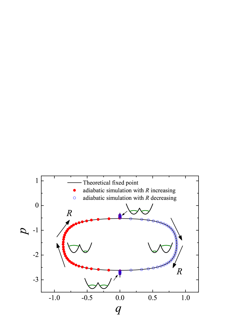
Figure 3: (color online) Solid lines depict phase space locations of fixed-point solutions for our model Hamiltonian in Eq. (4) as values of $R$ are scanned. The solid and empty dots represent the actual states of the system in numerical experiments of an adiabatic process, where $R$ is first increased from $R=-0.25<R_{1}$ to $R=0.25>R_{2}$, and then returns to $R=-0.25$, at a constant speed $V=10^{-6}$. Long arrows indicate the moving direction of the actual states as $R$ changes. The four double-well plots schematically show the symmetry-breaking consequence in the context of a two-mode BEC Hamiltonian. $c=0.2$, $\Delta=0.1$. Variables plotted here and in Fig. 4 are in dimensionless units.

Theory and numerical experiments – Applying the theory of IDF to the Hamiltonian in Eq. (4), one obtains $\langle\delta p\rangle=0$ and $\langle\delta q\rangle=-\frac{\Delta}{\sqrt{R^{2}+\Delta^{2}}}\frac{1}{R^{2}+\Delta^{2}-c\sqrt{R^{2}+\Delta^{2}}}\frac{dR}{dt}$ for $R<R_{1}$ notedivergence . Therefore, as $R$ increases from $R<R_{1}$, $\frac{dR}{dt}=V>0$, and $\langle\delta q\rangle$ is definitely negative. Returning to the phase space plot in Fig. 3, this means that if $R$ increases from $R<R_{1}$, the actual state (on average, to be more precise) is slightly left-shifted from the fixed point at $(0,\mu-\pi)$. So after passing the bifurcation at $R=R_{1}$, the system is expected to adiabatically follow the left symmetry-breaking solution $(\bar{q},\bar{p})=(-\eta,\mu-\pi)$ for $R_{1}<R<0$ and $(\bar{q},\bar{p})=(-\eta,\mu)$ for $0<R<R_{2}$. Similar theoretical results show that, if $R$ decreases from $R>R_{2}$, then the actual state must be slightly right-shifted from the fixed point at $(0,\mu)$, a prediction consistent with the above-mentioned $\mathcal{P}$$\mathcal{T}$ symmetry of the system. So after crossing the bifurcation point at $R=R_{2}$, the system should adiabatically follow the other symmetry-breaking solution $(\bar{q},\bar{p})=(\eta,\mu)$ for $0<R<R_{2}$ and $(\bar{q},\bar{p})=(\eta,\mu-\pi)$ for $R_{1}<R<0$. As shown in Fig. 3 (solid or empty dots), our numerical results based only on Hamilton’s equation of motion confirm this prediction. For the results shown we have set $V=10^{-6}$ to ensure a slow process. Indeed, at all times the difference between the actual states (dots) and the instantaneous fixed points (solid lines) is invisible to our naked eyes. Yet, the small IDF does assist in a symmetry-breaking choice regarding which of two stable fixed-point solutions is adiabatically followed by the system. In the language of $\hat{H}_{\text{m}}$, after the system passes the bifurcation at $R=R_{1}$ owing to an increasing $R$, $q=|b|^{2}-|a|^{2}$ becomes appreciably negative, so one mode develops more population than the other, signaling a clear delocalization-localization transition induced by IDF. The opposite population imbalance occurs when the system passes the bifurcation at $R=R_{2}$ with a decreasing $R$. Furthermore, joining these two manipulation steps together so that $R$ returns to its very original value in the end (which is already the case in Fig. 3), we clearly observe the formation of an adiabatic “hysteresis” loop in phase space. That is, by increasing and then decreasing $R$, a navigation loop in phase space is formed because the adiabatic following in the forward step and backward step lands on different symmetry-breaking branches note .

There is one subtle point to be clarified: Our theory of IDF [see (Eq. 2)] is about quantities $\langle\delta q\rangle$ averaged over all initial conditions of $(\delta q,\delta p)$, but what determines the adiabatic following is the actual $\delta q$ in a single process. The Supplementary Material contains a detailed analysis on this point. In particular, we show that if initially there is a deviation of $\delta q$ from $\langle\delta q\rangle$, then the difference $\delta q-\langle\delta q\rangle$ oscillates with time and later, as $R$ approaches the bifurcation point, this deviation becomes negligible as compared with $\langle\delta q\rangle$. It is for this reason that the definite sign of $\langle\delta q\rangle$ is equivalent to the definite sign of $\delta q$, which hence justifies our theory based on $\langle\delta q\rangle$.

Berry phase generation via one single-valued parameter – As a final interesting concept, we discuss the generation of a Berry phase using one single-valued adiabatic parameter $R$. This is made possible by IDF and bifurcations. In particular, the navigation loop in Fig. 3 shows that the time-evolving states of $\hat{H}_{\text{m}}$ trace out a nontrivial geometry after increasing $R$ from $R<R_{1}$ to $R>R_{2}$ and then returning $R$ to its initial value. Let $|\psi_{\text{left}}\rangle$ and $|\psi_{\text{right}}\rangle$ be the eigenstates of $\hat{H}_{\text{m}}$ (with $R_{1}<R<R_{2}$) mapped from the left and right fixed-point solutions of $H$. Assuming exact adiabatic following with the instantaneous adiabatic eigenstates, the Berry phase generated along the navigation loop is analytically found to be

$$\beta_{\text{Berry}} = i\int_{R_{\text{1}}}^{R_{\text{2}}}dR\left(\langle\psi_{\text{left}}|\frac{d}{dR}|\psi_{\text{left}}\rangle-\langle\psi_{\text{right}}|\frac{d}{dR}|\psi_{\text{right}}\rangle\right)$$ (6)

$$= \pi(1-\Delta/c).$$

In our numerical experiments, we choose to integrate the Berry connection using the actual states during the physical process (this simple method will not account for the nonlinear Berry phase correction studied in Ref. liu ). It is found that for the shown regime in Fig. 4, the agreement between theory and simulations is excellent, with tiny but visible differences. Such visible differences remind us that a direct numerical integration of the Berry connection along the actual time evolution path is not necessarily reliable because it could accumulate the effect of IDF ZhangAOP2012 . Nevertheless, the fair agreement shown in Fig. 4 confirms our analytical result, demonstrates the feasibility of Berry phase generation using only one single-valued adiabatic parameter, and verifies from another angle that IDF is important for understanding adiabatic following in the presence of bifurcation.

Figure 4: Analytical and numerical Berry phase results vs $c$, for the quantum system described in Eq. (5) with $\Delta=0.1$. The theoretical results are from Eq. (6), while the numerical results are obtained directly by integrating the Berry connection along the actual path of adiabatic evolution.

Conclusion – Bifurcation greatly amplifies subtle intrinsic fluctuations that are beyond classical adiabatic invariants. This leads to a selection rule regarding which of two symmetry-connected stable fixed-point solutions may be adiabatically followed. In cases of multiple bifurcation points, adiabatic hysteresis loops in phase space and the generation of Berry phase by manipulating one single-valued parameter are also shown to be possible. Our findings are of fundamental interest to both classical systems and quantum many-body systems on the mean-field level. The implications of this work for symmetry breaking in fully quantum many-body systems should be a fascinating topic in our future studies.

Appendix

In this Appendix we discuss the difference between $\langle\delta q\rangle$ and $\delta q$, using the same notation as in the main text. It is important to clarify this point because our theory of intrinsic dynamical fluctuations (IDF) is about the quantity $\langle\delta q\rangle$ averaged over all initial conditions of $(\delta q,\delta p)$, but, as indicated in our main text, what determines the symmetry-breaking adiabatic following is the actual $\delta q$ in a single process without the averaging. Specifically, we need to show that, before the system crosses the bifurcation point, the (positive or negative) sign of $\delta q$ in an actual process is always the same as the sign of $\langle\delta q\rangle$ predicted by our theory. Without loss of generality we choose to discuss the case $R<R_{1}$ as an example.

For our model Hamiltonian, the $\Gamma$ matrix evaluated at the fixed point is found to have zero diagonal elements. Hence we can write it in the following form

$$\Gamma=\left(\begin{array}[]{cc}0&-A\\ B&0\end{array}\right).$$ (7)

Next we expand the Hamilton’s equation of motion to the first order of $\delta q$ and $\delta p$, we have

$$\left(\begin{array}[]{c}\frac{dp}{dt}\\ \frac{dq}{dt}\end{array}\right) = \left(\begin{array}[]{cc}0&-A\\ B&0\end{array}\right)\left(\begin{array}[]{c}\delta p\\ \delta q\end{array}\right)$$ (14)

$$= \left(\begin{array}[]{cc}0&-A\\ B&0\end{array}\right)\left(\begin{array}[]{c}p-\bar{p}\\ q-\bar{q}\end{array}\right),$$ (19)

where the instantaneous fixed point $(\bar{q},\bar{p})$ is located at $[0,\arctan(-\Delta/R)-\pi]$. Note that in general the off-diagonal elements $A$ and $B$ are $R$-dependent. Nevertheless, to gain physical insights and to develop a simple analytical result from the above equation, we consider a small time segment during which the $\Gamma$ matrix can be regarded as a constant, and $\bar{p}$ moves at a rate $M$ due to an increasing $R$. We then obtain

$$\frac{dp}{dt} = -Aq;$$

$$\frac{dq}{dt} = Bp-BMt,$$ (20)

a first-order differential equation that can be integrated directly. Upon direct integration we find the analytic solution

$$q = D\cos(\sqrt{AB}t)-\frac{M}{A}$$

$$p = -AD\sin(\sqrt{AB}t)+Mt,$$ (21)

where $D$ is one integration constant. This then indicates

$$\delta q = D\cos(\sqrt{AB}t)-\frac{M}{A};$$

$$\delta p = -AD\sin(\sqrt{AB}t).$$ (22)

Equation (22) clearly shows that $\delta q$ and $\delta p$ are oscillating solutions. In particular, the oscillation amplitude in $\delta q$ is seen to be the initial difference between $\delta q$ and the averaged quantity $\langle\delta q\rangle=-M/A$ (for the concerned time segment). Even more importantly, as the system approaches the bifurcation point at $R=R_{1}$, the term $-M/A$ is the dominating term because $|A|$ sharply decreases for $R$ approaching $R_{1}$. This makes it clear that the sign of $\delta q$ must agree perfectly with the sign of $\langle\delta q\rangle$.

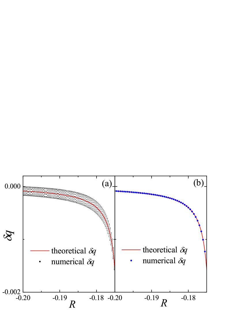
Figure 5: (color online) Comparison between numerical results of $\delta q$ and theoretical $\langle\delta q\rangle$ obtained from theory of IDF. System parameters are $c=0.2$, $\Delta=0.1$, and $\frac{dR}{dt}=10^{-6}$. (a) Initially the canonical variables $(q,p)$ are set exactly on the instantaneous fixed point. The initial $\delta q$ is hence zero, which differs from the theoretical nonzero $\langle\delta q\rangle$. (b) Initially $\delta p$ and $\delta q$ are precisely chosen according to the theory of IDF (see the main text). In this case, $\delta q$ is seen to agree with $\langle\delta q\rangle$ at all times before the bifurcation, which is about to occur at $R=-0.173$ for parameters used here.

To verify this theoretical understanding, we performed numerical experiments and quantitatively compare in Fig. 5 the numerically found $\delta q$ with $\langle\delta q\rangle$ obtained from the theory of IDF (see the main text), for an increasing $R$ ($R<R_{1}$). As seen in Fig. 5(a), the actual numerical $\delta q$ indeed oscillates around theoretical $\langle\delta q\rangle$. As $R$ approaches closer to $R_{1}=-0.173$ (beyond the shown regime of $R$ in Fig. 5), the oscillations of $\delta q$ around $\langle\delta q\rangle$ remain small and yet $\langle\delta q\rangle$ becomes more and more negative. Therefore, the sign of $\delta q$ is always identical with the sign of $\langle\delta q\rangle$ when the system is close to bifurcation crossing. As a second confirmation of our insights above, Fig. 5(b) shows that, if initially we set $\delta q=\langle\delta q\rangle$ and $\delta p=\langle\delta p\rangle$, then the ensuing time dependence of $\delta q$ as found from our numerical calculation agrees exactly with that from the theory of IDF.

We finally note that, the ultimate reason why our analytical solution above for $(\delta q,\delta p)$ during a small time segment is already so useful is again linked with adiabatic following. That is, since $R$ changes slowly, the off-diagonal elements of $\Gamma$ and $M$ will all change slowly, and hence the equation of motion for $\delta q$, or for the deviation $\delta q-\langle\delta q\rangle$, is expected to adiabatically follow the solution given in Eq. (22). This is interesting because it suggests a theory of higher-order fluctuations in the intrinsic fluctuations.

References

- (1) P.A.M. Dirac, Proc. R. Soc. 107, 725 (1925); M. Born and V. A. Fock, Zeitschrift für Physik A 51, 165 (1928).
- (2) M. C. Gutzwiller, Chaos in Classical and Quantum Mechanics (Springer-Verlag, New York 1990), pp208-211.
- (3) K. P. Marzlin and B. C. Sanders, Phys. Rev. Lett. 93, 160408 (2004); Z. Y. Wu and H. Yang, Phys. Rev. A 72, 012114 (2005); R. Mackenzie, E. Marcotte, and H. Paquette, Phys. Rev. A 73, 042104 (2006); J. Ma, Y. P. Zhang, E. G. Wang, and B. Wu, Phys. Rev. Lett. 97, 128902 (2006); D. M. Tong, K. Singh, L. C. Kwek, and C. H. Oh, Phys. Rev. Lett. 95, 110407 (2005); D. M. Tong, K. Singh L. C. Kwek, and C. H. Oh, Phys. Rev. Lett. 98, 150402 (2007); D. M. Tong, Phys. Rev. Lett. 104, 120401 (2010).
- (4) Q. Zhang, J. B. Gong, and C. H. Oh, Ann. Phys. 327, 1202 (2012); Q. Zhang, J. Phys. A 45, 295302 (2012).
- (5) M. V. Berry and M. A. Morgan, Nonlinearity 9, 787 (1996).
- (6) A. D. A. M. Spallicci, A. Morbidelli, and G. Metris, Nonlinearity 18, 45 (2005).
- (7) M. V. Berry and J. M. Robbins, Proc. Roy. Soc. Lond. A442, 641 (1993).
- (8) J. Liu and L.B. Fu, Phys. Rev. A 81, 052112 (2010).
- (9) B. Wu and Q. Niu, Phys. Rev. A61, 023402 (2000).
- (10) X. Luo, Q. Xie, and B. Wu, Phys. Rev. A 77, 053601 (2008).
- (11) L. Morales-Molina and S. Flach, New J. Phys. 10, 013008 (2008).
- (12) C. H. Lee, Phys. Rev. Lett. 102, 070401 (2009); C. H. Lee, W. H. Hai, L. Shi, and K. L. Gao, Phys. Rev. A69, 033611 (2004).
- (13) Q. Zhang, P. Hänggi, and J. B. Gong, Phys. Rev. A 77, 053607 (2008).
- (14) D. F. Ye, L. B. Fu, and J. Liu, Phys. Rev. A77, 013402 (2008); L. B. Fu, D. F .Ye, C. H. Lee, W. P. Zhang, and J. Liu, Phys. Rev. A80, 013619 (2009).
- (15) J. Denschlag et al, Science 287, 97 (2000).
- (16) Y. V. Kartashov and V. A. Vysloukh, Opt. Lett. 34, 3544 (2009).
- (17) The expression of diverges at , because in our model, diverges at isolated points or . Such unphysical divergence can be removed by considering a second order expansion of and (which then predicts that and can be of the order of ). This procedure is unnecessary here because we do not need to estimate the precise magnitude of to make symmetry-breaking predictions (rather, only its sign is crucial).
- (18) A preliminary observation as a side result in a driven two-mode system in Ref. ZhangPRA2008 (coauthored by two of us) also suggested the possibility of adiabatic hysteresis loops. However, therein the origin of symmetry breaking was not well understood due to the lack of connection with IDF.