Sparsity-Aware Learning and Compressed Sensing: An Overview

1 Introduction

The notion of regularization has been widely used as a tool to address a number of problems that are usually encountered in Machine Learning. Improving the performance of an estimator by shrinking the norm of the MVU estimator, guarding against overfitting, coping with ill-conditioning, providing a solution to an underdetermined set of equations, are some notable examples where regularization has provided successful answers. A notable example is the ridge regression concept, where the LS loss function is combined, in a tradeoff rationale, with the Euclidean norm of the desired solution.

In this paper, our interest will be on alternatives to the Euclidean norms and in particular the focus will revolve around the $\ell_{1}$ norm; this is the sum of the absolute values of the components comprising a vector. Although seeking a solution to a problem via the $\ell_{1}$ norm regularization of a loss function has been known and used since the 1970s, it is only recently that has become the focus of attention of a massive volume of research in the context of compressed sensing. At the heart of this problem lies an underdetermined set of linear equations, which, in general, accepts an infinite number of solutions. However, in a number of cases, an extra piece of information is available: the true model, whose estimate we want to obtain, is sparse; that is, only a few of its coordinates are nonzero. It turns out that a large number of commonly used applications can be cast under such a scenario and can be benefited by a so-called sparse modeling.

Besides its practical significance, sparsity-aware processing has offered to the scientific community novel theoretical tools and solutions to problems that only a few years ago seemed to be intractable. This is also a reason that this is an interdisciplinary field of research encompassing scientists from, e.g., mathematics, statistics, machine learning, signal processing. Moreover, it has already been applied in many areas ranging from biomedicine, to communications and astronomy. At the time this paper is compiled, there is a “research happening” in this field, which poses some difficulties in assembling related material together. We have made an effort to put together, in a unifying way, the basic notions and ideas that run across this new field. Our goal is to provide the reader with an overview of the major contributions which took place in the theoretical and algorithmic fronts and have been consolidated over the last decade or so. Besides the methods and algorithms which are reviewed in this article, there is another path of methods based on the Bayesian learning rationale. Such techniques will be reviewed elsewhere.

2 Parameter Estimation

Parameter estimation is at the heart of what is known as Machine Learning; a term that is used more and more as an umbrella for a number of scientific topics that have evolved over the years within different communities, such as Signal Processing, Statistical Learning, Estimation/Detection, Control, Neurosciences, Statistical Physics, to name but a few.

In its more general and formal setting, the parameter estimation task is defined as follows. Given a set of data points $(y_{n},\bm{x}_{n})$, $y_{n}\in{\mathcal{R}},~{}\bm{x}_{n}\in{\mathcal{R}}^{l},~{},~{}n=1,2,\ldots,N$, known as the training data, and a parametric set of functions

$${\mathcal{F}}:=\{f_{\bm{\theta}},~{}\bm{\theta}\in{\mathcal{A}}\subseteq{\mathcal{R}}^{k}\},$$

find a function in ${\mathcal{F}}$, which will be denoted as $f(\cdot):=f_{\bm{\theta}_{*}}(\cdot)$, such that given the value of $\bm{x}\in{\mathcal{R}}^{l}$, $f(\bm{x})$ best approximates the corresponding value of $y\in{\mathcal{R}}$. After all, the main goal of Machine Learning is prediction. In a more general setting, $y$ can also be a vector $\bm{y}\in{\mathcal{R}}^{m}$. Most of our discussion here will be limited to real valued variables. Obviously, extensions to complex valued data are readily available.

Having adopted the parametric set of functions and given the the training data set, the goal becomes that of estimating the values of the parameters $\bm{\theta}$ so that to “fit” the data in some (optimal) way. There are various paths to achieve this goal. In this paper, our approach comprises the adoption of a loss function

$${\mathcal{L}}(\cdot,\cdot):~{}{\mathcal{R}}\times{\mathcal{R}}\longmapsto[0,\infty),$$

and obtain $\bm{\theta}_{*}$ such that

$$\bm{\theta}_{*}:=\operatorname{arg\,min}_{\bm{\theta}}J(\bm{\theta}),$$

where

$$J(\bm{\theta}):=\sum_{n=1}^{N}{\mathcal{L}}(y_{n},f_{\bm{\theta}}(\bm{x})).$$ (1)

In this review article, the focus will be on the Least Squares loss function, i.e.,

$${\mathcal{L}}(y,f_{\bm{\theta}}(\bm{x})):=(y-f_{\bm{\theta}}(\bm{x}))^{2}.$$

Among the many parametric models, regression covers a large class of Machine Learning tasks. In linear regression, one models the relationship of a dependent variable $y$, which is considered as the output of a system, with a set independent variables, $x_{1},x_{2},\ldots,x_{l}$, which are thought as the respective inputs that activate the system in the presence of a noise (unobserved) disturbance, $\eta$, i.e.,

$$y=\theta_{1}x_{1}+\ldots+\theta_{l}x_{l}+\theta_{0}+\eta,$$

where $\theta_{0}$ is known as the bias or intercept, see Figure 1. Very often the previous input-output relationship is written as

$$y=\bm{x}^{T}\bm{\theta}+\eta$$ (2)

where

$$\bm{\theta}:=[\theta_{1},\ldots,\theta_{0}]^{T},~{}~{}\mbox{and}~{}~{}\bm{x}:=[x_{1},\ldots,x_{l},1]^{T}.$$ (3)

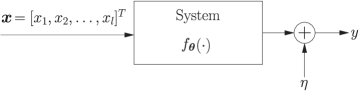
Figure 1: Block diagram showing the input-output relation in a regression model.

Often, $\bm{x}$ is called the regressor. Given the set of training data points, $(y_{n},\bm{x}_{n}),~{}n=1,2,\ldots,N$, (2) can compactly written as

$$\bm{y}=X\bm{\theta}+\bm{\eta}$$ (4)

where

$$X:=\left[\begin{array}[]{c}\bm{x}_{1}^{T}\\ \vdots\\ \bm{x}_{N}^{T}\end{array}\right],~{}~{}\bm{y}=\left[\begin{array}[]{c}y_{1}\\ \vdots\\ y_{N}\end{array}\right],~{}~{}\bm{\eta}=\left[\begin{array}[]{c}\eta_{1}\\ \vdots\\ \eta_{N}\end{array}\right].$$ (5)

For such a model, the Least Squares cost function becomes

$$J(\bm{\theta})=\sum_{n=1}^{N}(y_{n}-\bm{\theta}^{T}\bm{x}_{n})^{2}=||\bm{y}-X\bm{\theta}||^{2},$$ (6)

where $||\cdot||$ denotes the Euclidean norm. Minimizing (6) with respect to $\bm{\theta}$ results to the celebrated LS estimate

$$\hat{\bm{\theta}}_{LS}=(X^{T}X)^{-1}X^{T}\bm{y},$$ (7)

assuming the the matrix inversion is possible. However, for many practical cases, the cost function in (6) is augmented with a so called regularization term. There are a number of reasons that justify the use of a regularization term. Guarding against overfitting, purposely introducing bias in the estimator in order to improve the overall performance, dealing with the ill conditioning of the task are examples in which the use of regularization addresses successfully. Ridge regression is a celebrated example, where the cost function is augmented as

$$J(\bm{\theta})=||\bm{y}-X\bm{\theta}||^{2}+\lambda||\bm{\theta}||^{2},~{}\lambda\geq 0$$

leading to the estimate

$$\hat{\bm{\theta}}_{R}=(X^{T}X+\lambda I)^{-1}X^{T}\bm{y},$$

where $I$ is the identity matrix.

The major goal of this review article is to focus at alternative norms in place of the Euclidean norm, which was employed in ridge regression. As we will see, there are many good reasons in doing that.

3 Searching for a Norm

Mathematicians have been very imaginative in proposing various norms in order to equip linear spaces. Among the most popular norms used in functional analysis are the so-called $\ell_{p}$ norms. To tailor things to our needs, given a vector $\bm{\theta}\in\mathcal{R}^{l}$, its $\ell_{p}$ norm is defined as

$$\left\|{\bm{\theta}}\right\|_{p}\coloneqq\left(\sum_{i=1}^{l}|\theta_{i}|^{p}\right)^{\frac{1}{p}}.$$ (8)

For $p=2$, the Euclidean or $\ell_{2}$ norm is obtained, and for $p=1$, (8) results in the $\ell_{1}$ norm, i.e.,

$$\left\|{\bm{\theta}}\right\|_{1}=\sum_{i=1}^{l}|\theta_{i}|.$$ (9)

If we let $p\rightarrow\infty$, then we get the $\ell_{\infty}$ norm; let $|\theta_{i_{\max}}|\coloneqq\max\left\{|\theta_{1}|,|\theta_{2}|,\ldots,|\theta_{l}|\right\}$, and notice that

$$\left\|{\bm{\theta}}\right\|_{\infty}\coloneqq\lim_{p\rightarrow\infty}\left(|\theta_{i_{\max}}|^{p}\sum_{i=1}^{l}\left(\frac{|\theta_{i}|}{|\theta_{i_{\max}}|}\right)^{p}\right)^{\frac{1}{p}}=|\theta_{i_{\max}}|,$$ (10)

that is, $\left\|{\bm{\theta}}\right\|_{\infty}$ is equal to the maximum of the absolute values of the coordinates of $\bm{\theta}$. One can show that all the $\ell_{p}$ norms are true norms for $p\geq 1$; they satisfy all four requirements that a function $\mathcal{R}^{l}\rightarrow[0,\infty)$ must respect in order to be called a norm, i.e.,

1. $\left\|{\bm{\theta}}\right\|_{p}\geq 0$.

2. $\left\|{\bm{\theta}}\right\|_{p}=0\Leftrightarrow\bm{\theta}=\bm{0}$.

3. $\left\|{\alpha\bm{\theta}}\right\|_{p}=|\alpha|\left\|{\bm{\theta}}\right\|_{p}$, $\forall\alpha\in\mathcal{R}$.

4. $\left\|{\bm{\theta}_{1}+\bm{\theta}_{2}}\right\|_{p}\leq\left\|{\bm{\theta}_{1}}\right\|_{p}+\left\|{\bm{\theta}_{2}}\right\|_{p}$.

The third condition enforces the norm function to be (positively) homogeneous and the fourth one is the triangle inequality. These properties also guarantee that any function that is a norm is also a convex one. Although strictly speaking, if we allow $p>0$ to take values less than one in (8), the resulting function is easily shown not to be a true norm, we can still call them norms, albeit knowing that this is an abuse of the definition of a norm. An interesting case, which will be used extensively in this paper, is the $\ell_{0}$ norm, which can be obtained as the limit, for $p\rightarrow 0$, of

$$\left\|{\bm{\theta}}\right\|_{0}\coloneqq\lim_{p\rightarrow 0}\left\|{\bm{\theta}}\right\|^{p}_{p}=\lim_{p\rightarrow 0}\sum_{i=1}^{l}|\theta_{i}|^{p}=\sum_{i=1}^{l}\chi_{(0,\infty)}(|\theta_{i}|),$$ (11)

where $\chi_{\mathcal{A}}(\cdot)$ is the characteristic function with respect to a set $\mathcal{A}$, defined as

$$\chi_{\mathcal{A}}(\tau)\coloneqq\begin{cases}1,&\text{if}\ \tau\in\mathcal{A},\\ 0,&\text{if}\ \tau\notin\mathcal{A}.\end{cases}$$

That is, the $\ell_{0}$ norm is equal to the number of nonzero components of the respective vector. It is very easy to check that this function is not a true norm. Indeed, this function is not homogeneous, i.e., $\left\|{\alpha\bm{\theta}}\right\|_{0}\neq|\alpha|\left\|{\bm{\theta}}\right\|_{0}$, $\forall\alpha\neq 1$. Fig. 2 shows the isovalue curves, in the two-dimensional space, that correspond to $\left\|{\bm{\theta}}\right\|_{p}=\rho\equiv 1$, for $p=0,0.5,1,2$, and $\infty$. Observe that for the Euclidean norm the isovalue curve has the shape of a “ball” and for the $\ell_{1}$ norm the shape of a rhombus. We refer to them as the $\ell_{2}$ and the $\ell_{1}$ balls, respectively, by slightly “abusing” the meaning of a ball. Observe that in the case of the $\ell_{0}$ norm, the isovalue curve comprises both the horizontal and the vertical axes, excluding the $(0,0)$ element. If we restrict the size of the $\ell_{0}$ norm to be less than one, then the corresponding set of points becomes a singleton, i.e., $(0,0)$. Also, the set of all the points that have $\ell_{0}$ norm less than or equal to two, is the $\mathcal{R}^{2}$ space. This, slightly “strange” behavior, is a consequence of the discrete nature of this “norm”.

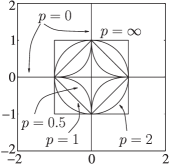
Figure 2: The isovalue curves for $\left\|{\theta}\right\|_{p}=1$ and for various values of $p$, in the two dimensional space. Observe that for the $\ell_{0}$ norm, the respective values cover the two axes with the exception of the point $(0,0)$. For the $\ell_{1}$ norm the isovalue curve is a rhombus and for the $\ell_{2}$ (Euclidean) norm, it is a circle.

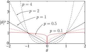
Figure 3: Observe that the epigraph, that is, the region above the graph, is nonconvex for values $p<1$, indicating the nonconvexity of the respective $|\cdot|^{p}$ function. The value $p=1$ is the smallest one for which convexity is retained. Also note that, for large values of $p>1$, the contribution of small values of $\theta$ to the respective norm becomes insignificant.

Fig. 3 shows the graph of $|\cdot|^{p}$, which is the individual contribution of each component of a vector to the $\ell_{p}$ norm, for different values of $p$. Observe that a) for $p<1$, the region which is formed above the graph (known as epigraph) is not a convex one, which verifies what we have already said; i.e, the respective function is not a true norm, b) for values of the argument $|\theta|>1$, the larger the value of $p\geq 1$ and the larger the value of $|\theta|$ the higher its respective contribution to the norm. Hence, if $\ell_{p}$ norms, $p\geq 1$, are used to regularize a loss function, such large values become the dominant ones and the optimization algorithm will concentrate on these by penalizing them to get smaller, so that the overall cost to be reduced. On the other hand, for values of the argument $|\theta|<1$ and closer to zero, the $\ell_{1}$ norm is the only one (among $p\geq 1$) that retains relatively large values and, hence, the respective components can still have a say in the optimization process and can be penalized by being pushed to smaller values. Hence, if the $\ell_{1}$ norm is used to replace the $\ell_{2}$ one in the regularization equation, only those components of the vector, that are really significant in reducing the model misfit measuring term in the regularized cost function, will be kept and the rest will be forced to zero. The same tendency, yet more aggressive, is true for $0\leq p<1$. The extreme case is when one considers the $\ell_{0}$ norm. Even a small increase of a component from zero, makes its contribution to the norm large, so the optimizing algorithm has to be very “cautious” in making an element nonzero.

From all the true norms ($p\geq 1$), the $\ell_{1}$ is the only one that shows respect to small values. The rest of the $\ell_{p}$ norms, $p>1$, just squeeze them, to make their values even smaller and care, mainly, for the large values. We will return to this point very soon.

4 The Least Absolute Shrinkage and Selection Operator (LASSO)

We have already discussed some of the benefits in adopting the regularization method for enhancing the performance of an estimator. However, in this paper, we are going to see and study more reasons that justify the use of regularization. The first one refers to what is known as the interpretation power of an estimator. For example, in the regression task, we want to select those components, $\theta_{i}$, of $\bm{\theta}$ that have the most important say in the formation of the output variable. This is very important if the number of parameters, $l$, is large and we want to concentrate on the most important of them. In a classification task [Theo 09], not all features are informative, hence one would like to keep the most informative of them and make the less informative ones equal to zero. Another related problem refers to those cases where we know, a-priori, that a number of the components of a parameter vector are zero but we do not know which ones. The discussion we had at the end of the previous section starts now to become more meaningful. Can we use, while regularizing, an appropriate norm that can assist the optimization process a) in unveiling such zeros or b) to put more emphasis on the most significant of its components, those that play a decisive role in reducing the misfit measuring term in the regularized cost function, and set the rest of them equal to zero? Although the $\ell_{p}$ norms, with $p<1$, seem to be the natural choice for such a regularization, the fact that they are not convex makes the optimization process hard. The $\ell_{1}$ norm is the one that is “closest” to them yet it retains the computationally attractive property of convexity.

The $\ell_{1}$ norm has been used for such problems for a long time. In the seventies, it was used in seismology [Tayl 79, Clae 73], where the reflected signal, that indicates changes in the various earth substrates, is a sparse one, i.e., very few values are relatively large and the rest are small and insignificant. Since then, it has been used to tackle similar problems in different applications, e.g., [Sant 86, Dono 92]. However, one can trace two papers that were really catalytic in providing the spark for the current strong interest around the $\ell_{1}$ norm. One came from statistics, [Tibs 96], which addressed the LASSO task (first formulated, to our knowledge, in [Sant 86]), to be discussed next, and one from the signal analysis community, [Chen 98], which formulated the Basis Pursuit, to be discussed in a later section.

We first address our familiar regression task

$$\bm{y}=X\bm{\theta}+\bm{\eta},\quad\bm{y},\bm{\eta}\in{\cal R}^{N},\bm{\theta}\in{\cal R}^{l},$$

and obtain the estimate of the unknown parameter $\bm{\theta}$ via the LS loss, regularized by the $\ell_{1}$ norm, i.e., for $\lambda\geq 0$,

$$\hat{\bm{\theta}} \coloneqq \operatorname{arg\,min}_{\bm{\theta}\in\mathcal{R}^{l}}L(\bm{\theta},\lambda)$$

$$\coloneqq \operatorname{arg\,min}_{\bm{\theta}\in\mathcal{R}^{l}}\left(\sum_{n=1}^{N}(y_{n}-\bm{x}_{n}^{T}\bm{\theta})^{2}+\lambda\left\|{\bm{\theta}}\right\|_{1}\right)$$

$$= \operatorname{arg\,min}_{\bm{\theta}\in\mathcal{R}^{l}}\left((\bm{y}-X\bm{\theta})^{T}(\bm{y}-X\bm{\theta})+\lambda\left\|{\bm{\theta}}\right\|_{1}\right).$$ (13)

In order to simplify the analysis, we will assume hereafter, without harming generality, that the data are centered. If this is not the case, the data can be centered by subtracting the sample mean $\bar{y}$ from each one of the output values. The estimate of the bias term will be equal to the sample mean $\bar{y}$. The task in (13) can be equivalently written in the following two formulations

$$\hat{\bm{\theta}}:\min_{\bm{\theta}\in\mathcal{R}^{l}} (\bm{y}-X\bm{\theta})^{T}(\bm{y}-X\bm{\theta}),$$

s.t. $$\left\|{\bm{\theta}}\right\|_{1}\leq\rho,$$ (14)

or

$$\hat{\bm{\theta}}:\min_{\bm{\theta}\in\mathcal{R}^{l}} \left\|{\bm{\theta}}\right\|_{1},$$

s.t. $$(\bm{y}-X\bm{\theta})^{T}(\bm{y}-X\bm{\theta})\leq\epsilon,$$ (15)

given the user-defined parameters $\rho,\epsilon\geq 0$. The formulation in (14) is known as the LASSO and the one in (15) as the Basis Pursuit Denoising (BPDN), e.g., [Bruc 09]. All three formulations can be shown to be equivalent for specific choices of $\lambda,\epsilon$, and $\rho$. The minimized cost function in (13) corresponds to the Lagrangian of the formulations in (14) and (15). However, this functional dependence is hard to compute, unless the columns of $X$ are mutually orthogonal. Moreover, this equivalence does not necessarily imply that all three formulations are equally easy or difficult to solve. As we will see later on, algorithms have been developed along each one of the previous formulations. From now on, we will refer to all three formulations as the LASSO task, in a slight abuse of the standard terminology, and the specific formulation will be apparent from the context, if not stated explicitly.

As it was discussed before, the Ridge regression admits a closed form solution, i.e,

$$\hat{\bm{\theta}}_{R}=\left(X^{T}X+\lambda I\right)^{-1}X^{T}\bm{y}.$$

In contrast, this is not the case for LASSO and its solution requires iterative techniques. It is straightforward to see that LASSO can be formulated as a standard convex quadratic problem with linear inequalities. Indeed, we can rewrite (13) as

$$\min_{\{\theta_{i},u_{i}\}_{i=1}^{l}} (\bm{y}-X\bm{\theta})^{T}(\bm{y}-X\bm{\theta})+\lambda\sum_{i=1}^{l}u_{i}$$

s.t. $$\left\{\begin{aligned} &-u_{i}\leq\theta_{i}\leq u_{i},\\ &u_{i}\geq 0,\end{aligned}\quad i=1,2,\ldots,l,\right.$$

which can be solved by any standard convex optimization method, e.g., [Ye 97, Boyd 04]. The reason that developing algorithms for the LASSO has been a hot research topic is due to the emphasis in obtaining efficient algorithms by exploiting the specific nature of this task, especially for cases where $l$ is very large, as it is often the case in practice.

In order to get a better insight of the nature of the solution that is obtained by LASSO, let us assume that the regressors are mutually orthogonal and of unit norm, hence $X^{T}X=I$. Orthogonality of the input matrix helps to decouple the coordinates and results to $l$ one-dimensional problems, that can be solved analytically. For this case, the LS estimator becomes

$$\hat{\bm{\theta}}_{\text{LS}}=(X^{T}X)^{-1}X^{T}\bm{y}=X^{T}\bm{y},$$

and the ridge regression gives

$$\hat{\bm{\theta}}_{R}=\frac{1}{1+\lambda}\hat{\bm{\theta}}_{\text{LS}},$$ (16)

that is, every component of the LS estimator is simply shrunk by the same factor, $\frac{1}{1+\lambda}$.

In the case of the $\ell_{1}$ regularization, the minimized Lagrangian function is no more differentiable, due to the presence of the absolute values in the $\ell_{1}$ norm. So, in this case, we have to consider the notion of the subdifferential (see Appendix). It is known that if the zero vector belongs to the subdifferential set of a convex function at a point, this means that this point corresponds to a minimum of the function. Taking the subdifferential of the Lagrangian defined in (13) and recalling that the subdifferential of a differentiable function includes only the respective gradient, we obtain that

$$\bm{0}\in-2X^{T}\bm{y}+2X^{T}X\bm{\theta}+\lambda\partial\left\|{\bm{\theta}}\right\|_{1},$$

where $\partial$ stands for the subdifferential operator (see Appendix). If $X$ has orthonormal columns, the previous equation can be written component-wise as follows

$$0\in-\hat{\theta}_{\text{LS},i}+\hat{\theta}_{1,i}+\frac{\lambda}{2}\partial\left|\hat{\theta}_{1,i}\right|,\quad\forall i,$$ (17)

where the subdifferential of the function $|\cdot|$, derived in Appendix, is given as

$$\partial|\theta|=\begin{cases}\{1\},&\text{if}\ \theta>0,\\ \{-1\},&\text{if}\ \theta<0,\\ [-1,1],&\text{if}\ \theta=0.\end{cases}$$

Thus, we can now write

$$\hat{\theta}_{1,i}= \hat{\theta}_{\text{LS},i}-\frac{\lambda}{2}, \hat{\theta}_{1,i}>0$$ if , (18)

$$\hat{\theta}_{1,i}= \hat{\theta}_{\text{LS},i}+\frac{\lambda}{2}, \hat{\theta}_{1,i}<0$$ if . (19)

Notice that (18) can only be true if $\hat{\theta}_{\text{LS},i}>\frac{\lambda}{2}$, and (19) only if $\hat{\theta}_{\text{LS},i}<-\frac{\lambda}{2}$. Moreover, in the case where $\hat{\theta}_{1,i}=0$, then (17) and the subdifferential of $|\cdot|$ suggest that necessarily $\left|\hat{\theta}_{\text{LS},i}\right|\leq\frac{\lambda}{2}$. Concluding, we can write in a more compact way that

$$\hat{\theta}_{1,i}=\operatorname{sgn}(\hat{\theta}_{\text{LS},i})\left(\left|\hat{\theta}_{\text{LS},i}\right|-\frac{\lambda}{2}\right)_{+},$$ (20)

where $(\cdot)_{+}$ denotes the “positive part” of the respective argument; it is equal to the argument if this is non-negative, and zero otherwise. This is very interesting indeed. In contrast to the ridge regression that shrinks all coordinates of the unregularized LS solution by the same factor, LASSO forces all coordinates, whose absolute value is less than or equal to $\lambda/2$, to zero, and the rest of the coordinates are reduced, in absolute value, by the same amount $\lambda/2$. This is known as soft thresholding, to distinguish it from the hard thresholding operation; the latter is defined as $\theta\cdot\chi_{(0,\infty)}\left(|\theta|-\frac{\lambda}{2}\right)$, $\theta\in\mathcal{R}$, where $\chi_{(0,\infty)}(\cdot)$ stands for the characteristic function with respect to the set $(0,\infty)$. Fig. 4 shows the graphs illustrating the effect that the ridge regression, LASSO and hard thresholding have on the unregularized LS solution, as a function of its value (horizontal axis). Note that our discussion here, simplified via the orthonormal input matrix case, has quantified what we had said before about the tendency of the $\ell_{1}$ norm to push small values to become exactly zero. This will be further strengthened, via a more rigorous mathematical formulation, in Section 6.

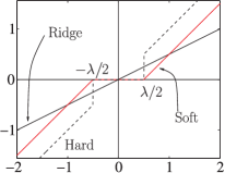
Figure 4: Output-input curves for the hard thresholding, soft thresholding operators together with the linear operator associated with the ridge regression, for the same value of $\lambda=1$.

Example 1.

Assume that the unregularized LS solution, for a given regression task, $\bm{y}=X\bm{\theta}+\bm{\eta}$, is given by:

$$\hat{\bm{\theta}}_{\text{LS}}=[0.2,-0.7,0.8,-0.1,1.0]^{T}.$$

Derive the solutions for the corresponding ridge regression and $\ell_{1}$ norm regularization tasks. Assume that the input matrix $X$ has orthonormal columns and that the regularization parameter is $\lambda=1$. Also, what is the result of hard thresholding the vector $\hat{\bm{\theta}}_{\text{LS}}$ with threshold equal to $0.5$?

We know that the corresponding solution for the ridge regression is

$$\hat{\bm{\theta}}_{R}=\frac{1}{1+\lambda}\hat{\bm{\theta}}_{\text{LS}}=[0.1,-0.35,0.4,-0.05,0.5]^{T}.$$

The solution for the $\ell_{1}$ norm regularization is given by soft thresholding, with threshold equal to $\lambda/2=0.5$, hence the corresponding vector is

$$\hat{\bm{\theta}}_{1}=[0,-0.2,0.3,0,0.5]^{T}.$$

The result of the hard thresholding operation is the vector $[0,-0.7,0.8,0,1.0]^{T}$.

Remarks 1.

• The hard and soft thresholding rules are only two possibilities out of a larger number of alternatives. Note that the hard thresholding operation is defined via a discontinuous function and this makes this rule to be unstable, in the sense of being very sensitive to small changes of the input. Moreover, this shrinking rule tends to exhibit large variance in the resulting estimates. The soft thresholding rule is a continuous function, but, as it is readily seen from the graph in Fig. 4, it introduces bias even for the large values of the input argument. In order to ameliorate such shortcomings, a number of alternative thresholding operators have been introduced and studied both theoretically and experimentally. Although these are not within the mainstream of our interest, we provide two popular examples for the sake of completeness; the Smoothly Clipped Absolute Deviation (SCAD):

  $$\hat{\theta}_{\text{SCAD}}=\begin{dcases}\operatorname{sgn}(\theta)\left(|\theta|-\lambda_{\text{SCAD}}\right)_{+},&|\theta|\leq 2\lambda_{\text{SCAD}},\\ \frac{(\alpha-1)\theta-\alpha\lambda_{\text{SCAD}}\operatorname{sgn}(\theta)}{\alpha-2},&2\lambda_{\text{SCAD}}<|\theta|\leq\alpha\lambda_{\text{SCAD}},\\ \theta,&|\theta|>\alpha\lambda_{\text{SCAD}},\end{dcases}$$

  and the nonnegative garrote thresholding rule :

  $$\hat{\theta}_{\text{garr}}=\begin{dcases}0,&|\theta|\leq\lambda_{\text{garr}},\\ \theta-\frac{\lambda_{\text{garr}}^{2}}{\theta},&|\theta|>\lambda_{\text{garr}}.\end{dcases}$$

  Fig. 5 shows the respective graphs. Observe that, in both cases, an effort has been made to remove the discontinuity (associated with the hard thresholding) and to remove/reduce the bias for large values of the input argument. The parameter $\alpha$ is a user-defined one. For a more detailed discussion on this topic, the interested reader can refer, for example, to [Anto 07].

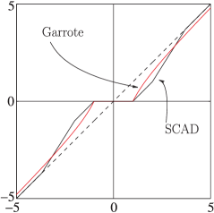
Figure 5: Output-input graph for the SCAD and nonnegative garotte rules with parameters $\alpha=3.7$, and $\lambda_{\text{SCAD}}=\lambda_{\text{garr}}=1$. Observe that both rules smooth out the discontinuity associated with the hard thresholding rule. Notice, also, that the SCAD rule removes the bias, associated with the soft thresholding rule, for large values of the input variable. On the contrary, the garrote thresholding rule allows some bias for large input values, which diminishes as $\lambda_{\text{garr}}$ gets smaller and smaller.

5 Sparse Signal Representation

In the previous section, we brought into our discussion the need for taking special care for zeros. Sparsity is an attribute that is met in a plethora of natural signals, since nature tends to be parsimonious. In this section, we will briefly present a number of application cases, where the existence of zeros in a mathematical expansion is of paramount importance, hence it justifies to further strengthen our search for and developing related analysis tools.

Echo cancelation is a major task in Communications. In a number of cases, the echo path, represented by a vector comprising the values of the impulse response samples, is a sparse one. This is the case, for example, in internet telephony and in acoustic and network environments, e.g., [Nayl 04, Bene 01, Aren 09]. Fig. 6 shows the impulse response of such an echo path. The impulse response of the echo path is of short duration; however, the delay with which it appears is not known. So, in order to model it, one has to use a long impulse response, yet only a relatively small number of the coefficients will be significant and the rest will be close to zero. Of course, one could ask why not use an LMS or an RLS [Hayk 96, Saye 03]and eventually the significant coefficients will be identified. The answer is that this turns out not to be the most efficient way to tackle such problems, since the convergence of the algorithm can be very slow. In contrast, if one embeds, somehow, into the problem the a-priori information concerning the existence of (almost) zero coefficients, then the convergence speed can be significantly increased and also better error floors can be attained.

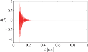
Figure 6: The impulse response function of an echo-path in a telephone network. Observe that although it is of relatively short duration, it is not a-priori known where exactly in time will occur.

A similar situation, as in the previous case, occurs in wireless communication systems, which involve multipath channels. A typical application is in high definition television (HDTV) systems, where the involved communications channels consist of a few non-negligible echoes, some of which may have quite large time delays with respect to the main signal, see, e.g. [Ghos 98, Cott 00, Ariy 97, Rond 03]. If the information signal is transmitted at high symbol rates through such a dispersive channel, then the introduced intersymbol interference (ISI) has a span of several tens up to hundreds of symbol intervals. This in turn implies that quite long channel estimators are required at the receiver’s end in order to reduce effectively the ISI component of the received signal, although only a small part of it has values substantially different to zero. The situation is even more demanding whenever the channel frequency response exhibits deep nulls. More recently, sparsity has been exploited in channel estimation for multicarrier systems, both for single antenna as well as for MIMO systems [Eiwe 10a, Eiwe 10b]. A thorough and in depth treatment related to sparsity in multipath communication systems is provided in [Bajw 10].

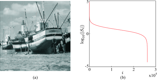
Figure 7: (a) A $512\times 512$ pixel image and (b) The magnitude of its Discrete Cosine Transform components in descending order and logarithmic scale. Note that more than $95\%$ of the total energy is contributed by only the $5\%$ of the largest components

Another example, which might be more widely known, is that of signal compression. It turns out that if the signal modalities, with which we communicate, e.g., speech, and also we sense the world, e.g., images, audio, are transformed into a suitably chosen domain then they are sparsely represented; only a relatively small number of the signal components in this domain are large and the rest are close to zero. As an example, Fig. 7a shows an image and Fig. 7b the plot of the magnitude of the obtained Discrete Cosine Transform (DCT) components, which are computed by writing the corresponding image array as a vector in lexicographic order. Note that more than $95\%$ of the total energy is contributed by only the $5\%$ of the largest components. This is at the heart of any compression technique. Only the large coefficients are chosen to be coded and the rest are considered to be zero. Hence, significant gains are obtained in memory/bandwidth requirements while storing/transmitting such signals, without much perceptual loss. Depending on the modality, different transforms are used. For example, in JPEG-2000, an image array, represented in terms of a vector that contains the intensity of the gray levels of the image pixels, is transformed via the discrete wavelet transform (DWT) and results to a transform vector that comprises only a few large components. Such an operation is of the form

$$\bm{S}=\Phi^{H}\bm{s},\quad\bm{s},\bm{S}\in\mathcal{C}^{l},$$ (21)

where $\bm{s}$ is the vector of the “raw” signal samples, $\bm{S}$ the vector of the transformed ones, and $\Phi$ is the $l\times l$ transformation matrix. Often, this is an orthonormal matrix, $\Phi^{H}\Phi=I$. Basically, a transform is nothing else than a projection of a vector on a new set of coordinate axes, which comprise the columns of the transformation matrix $\Phi$. Celebrated examples of such transforms are the wavelet, the discrete Fourier (DFT) and the discrete cosine (DCT) transforms, e.g., [Theo 09]. In such cases, where the transformation matrix is orthonormal, one can write that

$$\bm{s}=\Psi\bm{S},$$ (22)

where $\Psi=\Phi$. Equation (21) is known as the analysis and (22) as the synthesis equation.

Compression via such transforms exploit the fact that many signals in nature, which are rich in context, can be compactly represented in an appropriately chosen basis, depending on the modality of the signal. Very often, the construction of such bases tries to “imitate” the sensory systems that the human (and not only) brain has developed in order to sense these signals; and we know that nature (in contrast to modern humans) does not like to waste resources. A standard compression task comprises the following stages: a) Obtain the $l$ components of $\bm{S}$, via the analysis step (21), b) keep the, say, $k$ most significant of them, c) code these values, as well as their respective locations in the transform vector $\bm{S}$, and d) obtain the (approximate) original signal $\bm{s}$, when needed (after storage or transmission), via the synthesis equation (22), where in place of $\bm{S}$ only its $k$ most significant components are used, which are the ones that were coded, while the rest are set equal to zero. However, there is something unorthodox in this process of compression, as it has been practised till very recently. One processes (transforms) large signal vectors of $l$ coordinates, where $l$ in practice can be quite large, and then uses only a small percentage of the transformed coefficients and the rest are simply ignored. Moreover, one has to store/transmit the location of the respective large coefficients that were finally coded. A natural question that is now raised is the following: Since $\bm{S}$ in the synthesis equation is (approximately) sparse, can one compute it via an alternative path than the analysis equation in (21)? The issue here is to investigate whether one could use a more informative way of obtaining measurements from the available raw data, so that less than $l$ measurements are sufficient to recover all the necessary information. The ideal case would be to be able to recover it via a set of $k$ such measurement samples, since this is the number of the significant free parameters. On the other hand, if this sounds a bit extreme, can one obtain $N$ ($k<N<l$) such signal-related measurements, from which one can obtain the $k$ needed components of $\bm{S}$? It turns out that such an approach is possible and it leads to the solution of an underdetermined system of linear equations, under the constraint that the unknown target vector is a sparse one. The importance of such techniques becomes even more apparent when, instead of an orthonormal basis, as discussed before, a more general type of expansion is adopted, in terms of what is known as overcomplete dictionaries.

A dictionary [Mall 93] is a collection of parameterized waveforms, which are discrete-time signal samples, represented as vectors $\bm{\psi}_{i}\in\mathcal{C}^{l}$, $i\in\mathcal{I}$. For example, the columns of a DFT or a DWT matrix comprise a dictionary. These are two examples of what is known as complete dictionaries, which consist of $l$ (orthonormal) vectors, i.e., a number equal to the length of the signal vector. However, in many cases in practice, using such dictionaries is very restrictive. Let us take, for example, a segment of audio signal, from a news media or a video, that needs to be processed. This consists, in general, of different types of signals, namely speech, music, environmental sounds. For each type of these signals, different signal vectors (dictionaries) may be more appropriate in the expansion for the analysis. For example, music signals are characterized by a strong harmonic content and the use of sinusoids seems to be best for compression, while for speech signals a Gabor type signal expansion (sinusoids of various frequencies weighted by sufficiently narrow pulses at different locations in time, [Coif 92, Theo 09]), may be a better choice. The same applies when one deals with an image. Different parts of an image, e.g., parts which are smooth or contain sharp edges, may demand a different expansion vector set, for obtaining the best overall performance. The more recent tendency, in order to satisfy such needs, is to use overcomplete dictionaries. Such dictionaries can be obtained, for example, by concatenating different dictionaries together, e.g., a DFT and a DWT matrix to result in a combined $l\times 2l$ transformation matrix. Alternatively, a dictionary can be “trained” in order to effectively represent a set of available signal exemblars, a task which is often referred to as dictionary learning [Tosi 11, Rubi 10, Yagh 09]. While using such overcomplete dictionaries, the synthesis equation takes the form

$$\bm{s}=\sum_{i\in\mathcal{I}}\theta_{i}\bm{\psi}_{i}.$$ (23)

Note that, now, the analysis is an ill-posed problem, since the elements $\{\bm{\psi}_{i}\}_{i\in\mathcal{I}}$ (usually called atoms) of the dictionary are not linearly independent, and there is not a unique set of coefficients $\{\theta_{i}\}_{i\in\mathcal{I}}$ which generates $\bm{s}$. Moreover, we expect most of these coefficients to be (nearly) zero. Note that, in such cases, the cardinality of ${\cal I}$ is larger than $l$. This necessarily leads to underdetermined systems of equations with infinite many solutions. The question that is now raised is whether we can exploit the fact that most of these coefficients are known to be zero, in order to come up with a unique solution, and if yes, under which conditions such a solution is possible?

Besides the previous examples, there is a number of cases where an underdetermined system of equations is the result of our inability to obtain a sufficiently large number of measurements, due to physical and technical constraints. This is for example the case in MRI imaging, which will be presented in more detail later on.

6 In Quest for the Sparsest Solution

Inspired by the discussion in the previous section, we now turn our attention to the task of solving underdetermined systems of equations, by imposing the sparsity constraint on the solution [Elad 10]. We will develop the theoretical set up in the context of the regression task and we will adopt the notation that has been adopted for this task. Moreover, we will adhere to the real data case, in order to simplify the presentation. The theory can be readily extended to the more general complex data case, see, e.g., [Wrig 09b, Male 11]. We assume that we are given a set of measurements, $\bm{y}\coloneqq[y_{1},y_{2},\ldots,y_{N}]^{T}\in\mathcal{R}^{N}$, according to the linear model

$$\bm{y}=X\bm{\theta},\quad\bm{y}\in\mathcal{R}^{N},\bm{\theta}\in\mathcal{R}^{l},l>N,$$ (24)

where $X$ is the $N\times l$ input matrix, which is assumed to be of full row rank, i.e., $\operatorname{rank}(X)=N$. Our starting point is the noiseless case. The system in (24) is an underdetermined one and accepts an infinite number of solutions. The set of possible solutions lies in the intersection of the $N$ hyperplanes in the $l$-dimensional space,

$$\bigl{\{}\bm{\theta}\in\mathcal{R}^{l}:y_{n}=\bm{x}^{T}_{n}\bm{\theta}\bigr{\}},\quad n=1,2,\ldots,N.$$

We know from geometry, that the intersection of $N$ non-parallel hyperplanes (which in our case is guaranteed by the fact that $X$ has been assumed to be full row rank, hence $\bm{x}_{n}$ are mutually independent) is a plane of dimensionality $l-N$ (e.g., the intersection of two (non-parallel) (hyper)planes in the 3-dimensional space is a straight line; that is, a plane of dimensionality equal to one). In a more formal way, the set of all possible solutions, to be denoted as $\Theta$, is an affine set. An affine set is the translation of a linear subspace by a constant vector. Let us pursue this a bit further, since we will need it later on.

Let the null space of $X$ be the set $\operatorname{null}(X)$, defined as the linear subspace

$$\operatorname{null}(X)=\left\{\bm{z}\in\mathcal{R}^{l}:X\bm{z}=\bm{0}\right\}.$$

Obviously, if $\bm{\theta}_{0}$ is a solution to (24), i.e., $\bm{\theta}_{0}\in\Theta$, then it is easy to verify that $\forall\bm{\theta}\in\Theta$, $X(\bm{\theta}-\bm{\theta}_{0})=\bm{0}$, or $\bm{\theta}-\bm{\theta}_{0}\in\operatorname{null}(X)$. As a result,

$$\Theta=\bm{\theta}_{0}+\operatorname{null}(X),$$

and $\Theta$ is an affine set. We also know from linear algebra basics, that the null space of a full row rank matrix, $N\times l$, $l>N$, is a subspace of dimensionality $l-N$. Fig. 8 illustrates the case for one measurement sample in the $2$-dimensional space, $l=2$ and $N=1$. The set of solutions $\Theta$ is a line, which is the translation of the linear subspace crossing the origin (the $\operatorname{null}(X)$). Therefore, if one wants to determine a single point that lies in the affine set of solutions, $\Theta$, then an extra constraint/a-priori knowledge has to be imposed

In the sequel, three such possibilities are examined.

6.0.1 The $\ell_{2}$ Norm Minimizer

Our goal now becomes to pick a point in (the affine set) $\Theta$, that corresponds to the minimum $\ell_{2}$ norm. This is equivalent to solving the following constrained task

$$\min_{\bm{\theta}\in\mathcal{R}^{l}} \left\|{\bm{\theta}}\right\|_{2}^{2}$$

s.t. $$\bm{x}^{T}_{n}\bm{\theta}=y_{n},\quad n=1,2,\ldots,N.$$ (25)

The previous optimization task accepts a unique solution given in closed form as

$$\hat{\bm{\theta}}=X^{T}\left(XX^{T}\right)^{-1}\bm{y}.$$ (26)

The geometric interpretation of this solution is provided in Fig. 8a, for the case of $l=2$ and $N=1$. The radius of the Euclidean norm ball keeps increasing, till it touches the plane that contains the solutions. This point is the one with the minimum $\ell_{2}$ norm or, equivalently, the point that lies closest to the origin. Equivalently, the point $\hat{\bm{\theta}}$ can be seen as the (metric) projection of $\bm{0}$ onto $\Theta$.

Minimizing the $\ell_{2}$ norm, in order to solve a linear set of underdetermined equations, has been used in various applications. The closest to us is in the context of determining the unknown coefficients in an expansion using an overcomplete dictionary of functions (vectors) [Daub 88]. A main drawback of this method is that it is not sparsity preserving. There is no guarantee that the solution in (26) will give zeros even if the true model vector $\bm{\theta}$ has zeros. Moreover, the method is resolution limited [Chen 98]. This means that, even if there may be a sharp contribution of specific atoms in the dictionary, this is not portrayed in the obtained solution. This is a consequence of the fact that the information provided by $XX^{T}$ is a global one, containing all atoms of the dictionary in an “averaging” fashion, and the final result tends to smooth out the individual contributions, especially when the dictionary is overcomplete.

6.0.2 The $\ell_{0}$ Norm Minimizer

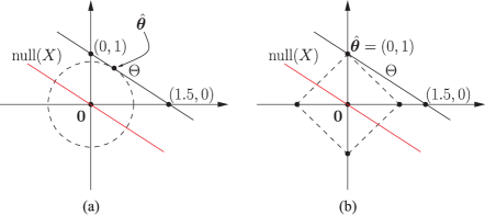
Figure 8: (a) The $\ell_{2}$ norm minimizer. The dotted circle corresponds to the smallest $\ell_{2}$ ball that intersects the set $\Theta$. As such, the intersection point, $\hat{\bm{\theta}}$, is the $\ell_{2}$ norm minimizer of the task (25). Notice that the vector $\hat{\bm{\theta}}$ contains no zero component. (b) The $\ell_{1}$ norm minimizer. The dotted rhombus corresponds to the smallest $\ell_{1}$ ball that intersects $\Theta$. Hence, the intersection point, $\hat{\bm{\theta}}$, is the solution of the constrained $\ell_{1}$ minimization task of (28). Notice that the obtained estimate $\hat{\bm{\theta}}=(0,1)$ contains a zero.

Now we turn our attention to the $\ell_{0}$ norm (once more, it is pointed out that this is an abuse of the definition of the norm, as stated before), and we make sparsity our new flag under which a solution will be obtained. Recall from Section 5 that such a constraint is in line with the natural structure that underlies a number of applications. The task now becomes

$$\min_{\bm{\theta}\in\mathcal{R}^{l}} \left\|{\bm{\theta}}\right\|_{0}$$

s.t. $$\bm{x}^{T}_{n}\bm{\theta}=y_{n},\quad n=1,2,\ldots,N,$$ (27)

that is, from all the points that lie on the plane of all possible solutions find the sparsest one; i.e., the one with the least number of nonzero elements. As a matter of fact, such an approach is within the spirit of Occam’s razor rule. It corresponds to the smallest number of parameters that can explain the obtained measurements. The points that are now raised are:

• Is a solution to this problem unique and under which conditions?

• Can a solution be obtained with low enough complexity in realistic time?

We postpone the answer to the first question later on. As for the second one, the news is no good. Minimizing the $\ell_{0}$ norm under a set of linear constraints is a task of combinatorial nature and as a matter of fact the problem is, in general, NP-hard [Nata 95]. The way to approach the problem is to consider all possible combinations of zeros in $\bm{\theta}$, removing the respective columns of $X$ in (24) and check whether the system of equations is satisfied; keep as solutions the ones with the smallest number of nonzero elements. Such a searching technique exhibits complexity of an exponential dependence on $l$. Fig. 8a illustrates the two points ($(1.5,0)$ and $(0,1)$) that comprise the solution set of minimizing the $\ell_{0}$ norm for the single measurement (constraint) case.

6.0.3 The $\ell_{1}$ Norm Minimizer

The current task is now given by

$$\min_{\bm{\theta}\in\mathcal{R}^{l}} \left\|{\bm{\theta}}\right\|_{1}$$

s.t. $$\bm{x}^{T}_{n}\bm{\theta}=y_{n},\quad n=1,2,\ldots,N.$$ (28)

Fig. 8b illustrates the geometry. The $\ell_{1}$ ball is increased till it touches the affine set of the possible solutions. For this specific geometry, the solution is the point $(0,1)$. In our discussion in Section 3, we saw that the $\ell_{1}$ norm is the one, out of all $\ell_{p}$, $p\geq 1$ norms, that bears some similarity with the sparsity favoring (nonconvex) $\ell_{p}$, $p<1$ “norms”. Also, we have commented that the $\ell_{1}$ norm encourages zeros, when the respective values are small. In the sequel, we will state one lemma, that establishes this zero-favoring property in a more formal way. The $\ell_{1}$ norm minimizer is also known as Basis Pursuit and it was suggested for decomposing a vector signal in terms of the atoms of an overcomplete dictionary [Chen 98].

The $\ell_{1}$ minimizer can be brought into the standard Linear Programming (LP) form and then can be solved by recalling any related method; the simplex method or the more recent interior point methods are two possibilities, see, e.g., [Boyd 04, Dant 63]. Indeed, consider the (LP) task

$$\min_{\bm{x}} \bm{c}^{T}\bm{x}$$

s.t. $$A\bm{x}=\bm{b}$$

$$\bm{x}\geq\bm{0}.$$

To verify that our $\ell_{1}$ minimizer can be cast in the previous form, notice first that any $l$-dimensional vector $\bm{\theta}$ can be decomposed as

$$\bm{\theta}=\bm{u}-\bm{v},\quad\bm{u}\geq\bm{0},\bm{v}\geq\bm{0}.$$

Indeed, this holds true if, for example,

$$\bm{u}\coloneqq\bm{\theta}_{+},\quad\bm{v}\coloneqq(-\bm{\theta})_{+},$$

where $\bm{x}_{+}$ stands for the vector obtained after taking the positive parts of the components of $\bm{x}$. Moreover, notice that

$$\left\|{\bm{\theta}}\right\|_{1}=[1,1,\ldots,1]\begin{bmatrix}\bm{\theta}_{+}\\ (-\bm{\theta})_{+}\end{bmatrix}=[1,1,\ldots,1]\begin{bmatrix}\bm{u}\\ \bm{v}\end{bmatrix}.$$

Hence, our $\ell_{1}$ minimization task can be recast in the LP form, if

$$\bm{c} \coloneqq[1,1,\ldots,1]^{T},\quad \bm{x} \coloneqq[\bm{u}^{T},\bm{v}^{T}]^{T},$$

$$A \coloneqq[X,-X], \bm{b} \coloneqq\bm{y}.$$

6.0.4 Characterization of the $\ell_{1}$ norm minimizer

Lemma 1.

An element $\bm{\theta}$ in the affine set, $\Theta$, of the solutions of the underdetermined linear system (24), has minimal $\ell_{1}$ norm if and only if the following condition is satisfied:

$$\left|\sum_{i:~{}\theta_{i}\neq 0}\operatorname{sgn}(\theta_{i})z_{i}\right|\leq\sum_{i:~{}\theta_{i}=0}|z_{i}|,\quad\forall\bm{z}\in\operatorname{null}(X).$$ (29)

Moreover, the $\ell_{1}$ minimizer is unique if and only if the inequality in (29) is a strict one for all $\bm{z}\neq\bm{0}$ (see, e.g., [Pink 89]).

Remarks 2.

The previous lemma has a very interesting and important consequence. If $\hat{\bm{\theta}}$ is the unique minimizer of (28), then

$$\operatorname{card}\{i:\hat{\theta}_{i}=0\}\geq\dim(\operatorname{null}(X)),$$ (30)

where $\operatorname{card}\{\cdot\}$ denotes the cardinality of a set. In words, the number of zero coordinates of the unique minimizer cannot be smaller than the dimension of the null space of $X$. Indeed, if this is not the case, then the unique minimizer could have less zeros than the dimensionality of $\operatorname{null}(X)$. As it can easily be shown, this means that we can always find a $\bm{z}\in\operatorname{null}(X)$, which has zeros in the same locations where the coordinates of the unique minimizer are zero, and at the same time it is not identically zero, i.e., $\bm{z}\neq\bm{0}$. However, this would violate (29), which in the case of uniqueness holds as a strict inequality.

Definition 1.

A vector $\bm{\theta}$ is called $k$-sparse if it has at most $k$ nonzero components.

Remarks 3.

If the minimizer of (28) is unique, then it is a $k$-sparse vector with

$$k\leq N.$$

This is a direct consequence of the Remark 2, and the fact that for the matrix $X$,

$$\dim(\operatorname{null}(X))=l-\operatorname{rank}(X)=l-N.$$

Hence, the number of the nonzero elements of the unique minimizer must be at most equal to $N$.

If one resorts to geometry, all the previously stated results become crystal clear.

6.0.5 Geometric interpretation

Assume that our target solution resides in the $3$-dimensional space and that we are given one measurement

$$y_{1}=\bm{x}_{1}^{T}\bm{\theta}=x_{11}\theta_{1}+x_{12}\theta_{2}+x_{13}\theta_{3}.$$

Then the solution lies in the $2$-dimensional (hyper)plane, which is described by the previous equation. To get the minimal $\ell_{1}$ solution we keep increasing the size of the $\ell_{1}$ ball (the set of all points that have equal $\ell_{1}$ norm) till it touches this plane. The only way that these two geometric objects have a single point in common (unique solution) is when they meet at a corner of the diamond. This is shown in Fig. 9a. In other words, the resulting solution is $1$-sparse, having two of its components equal to zero. This complies with the finding stated in Remark 3, since now $N=1$. For any other orientation of the plane, this will either cut across the $\ell_{1}$ ball or will share with the diamond an edge or a side. In both cases, there will be infinite many solutions.

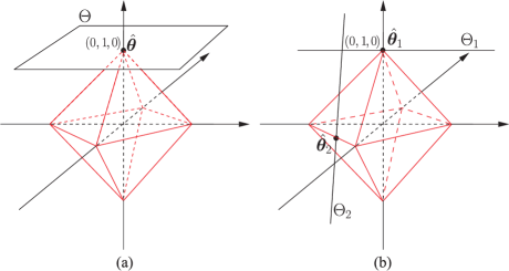
Figure 9: (a) The $\ell_{1}$ ball intersecting with a plane. The only possible scenario, for the existence of a unique common intersecting point of the $\ell_{1}$ ball with a plane in the Euclidean $\mathcal{R}^{3}$ space, is for the point to be located at one of the corners of the $\ell_{1}$ ball, i.e., to be an $1$-sparse vector. (b) The $\ell_{1}$ ball intersecting with lines. In this case, the sparsity level of the unique intersecting point is relaxed; it could be an $1$- or a $2$-sparse vector.

Let us now assume that we are given an extra measurement,

$$y_{2}=x_{21}\theta_{1}+x_{22}\theta_{2}+x_{23}\theta_{3}.$$

The solution now lies in the intersection of the two previous planes, which is a straight line. However, now, we have more alternatives for a unique solution. A line, e.g., $\Theta_{1}$, can either touch the $\ell_{1}$ ball at a corner ($1$-sparse solution) or, as it is shown in Fig. 9b, it can touch the $\ell_{1}$ ball at one of its edges, e.g., $\Theta_{2}$. The latter case, corresponds to a solution that lies on a $2$-dimensional subspace, hence it will be a $2$-sparse vector. This also complies with the findings stated in Remark 3, since in this case, we have $N=2$, $l=3$ and the sparsity level for a unique solution can be either $1$ or $2$.

Note that uniqueness is associated with the particular geometry and orientation of the affine set, which is the set of all possible solutions of the underdetermined system of equations. For the case of the square $\ell_{2}$ norm, the solution was always unique. This is a consequence of the (hyper)spherical shape formed by the Euclidean norm. From a mathematical point of view, the square $\ell_{2}$ norm is a strict convex function. This is not the case for the $\ell_{1}$ norm, which is convex, albeit not a strict convex function.

Example 2.

Consider a sparse vector parameter $[0,1]^{T}$, which we assume to be unknown. We will use one measurement to sense it. Based on this single measurement, we will use the $\ell_{1}$ minimizer of (28) to recover its true value. Let us see what happens. We will consider three different values of the “sensing” (input) vector $\bm{x}$ in order to obtain the measurement $y=\bm{x}^{T}\bm{\theta}$: a) $\bm{x}=[\frac{1}{2},1]^{T}$, b) $\bm{x}=[1,1]^{T}$, and c) $\bm{x}=[2,1]^{T}$. The resulting measurement, after sensing $\bm{\theta}$ by $\bm{x}$, is $y=1$ for all the three previous cases.

Case a): The solution will lie on the straight line

$$\Theta=\left\{[\theta_{1},\theta_{2}]^{T}\in\mathcal{R}^{2}:\frac{1}{2}\theta_{1}+\theta_{2}=1\right\},$$

which is shown in Fig. 10a. For this setting, expanding the $\ell_{1}$ ball, this will touch the line (our solutions’ affine set) at the corner $[0,1]^{T}$. This is a unique solution, hence it is sparse, and it coincides with the true value.

Case b): The solutions lies on the straight line

$$\Theta=\left\{[\theta_{1},\theta_{2}]^{T}\in\mathcal{R}^{2}:\theta_{1}+\theta_{2}=1\right\},$$

which is shown in Fig. 10b. For this set up, there is an infinite number of solutions, including two sparse ones.

Case c): The affine set of solutions is described by

$$\Theta=\left\{[\theta_{1},\theta_{2}]^{T}\in\mathcal{R}^{2}:2\theta_{1}+\theta_{2}=1\right\},$$

which is sketched in Fig. 10c. The solution in this case is sparse, but it is not the correct one.

This example is quite informative. If we sense (measure) our unknown parameter vector with appropriate sensing (input) data, the use of the $\ell_{1}$ norm can unveil the true value of the parameter vector, even if the system of equations is underdetermined, provided that the true parameter is sparse. This now becomes our new goal. To investigate whether what we have just said can be generalized, and under which conditions holds true, if it does. In such a case, the choice of the regressors (which we just called them sensing vectors) and hence the input matrix (which, from now on, we will refer to, more and more frequently, as the sensing matrix) acquire an extra significance. It is not enough for the designer to care only for the rank of the matrix, i.e., the linear independence of the sensing vectors. One has to make sure that the corresponding affine set of the solutions has such an orientation, so that the touch with the $\ell_{1}$ ball, as this increases from zero to meet this plane, is a “gentle” one, i.e., they meet at a single point, and more important at the correct one; that is, at the point that represents the true value of the sparse parameter, which we are searching for.

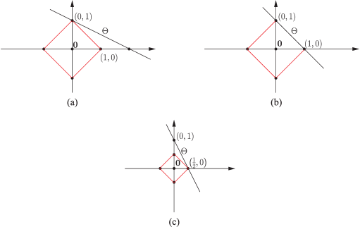
Figure 10: (a) Sensing with $\bm{x}=[\frac{1}{2},1]^{T}$, (b) sensing with $\bm{x}=[1,1]^{T}$, (c) sensing with $\bm{x}=[2,1]^{T}$. The choice of the sensing vector $\bm{x}$ is crucial to unveiling the true sparse solution $(0,1)$. Only the sensing vector $\bm{x}=[\frac{1}{2},1]^{T}$ identifies uniquely the desired $(0,1)$.

Remarks 4.

• Often in practice, the columns of the input matrix, $X$, are normalized to unit $\ell_{2}$ norm. Although $\ell_{0}$ norm is insensitive to the values of the nonzero components of $\bm{\theta}$, this is not the case with the $\ell_{1}$ and $\ell_{2}$ norms. Hence, while trying to minimize the respective norms, and at the same time to fulfill the constraints, components that correspond to columns of $X$ with high energy (norm) are favored more than the rest. Hence, the latter become more popular candidates to be pushed to zero. In order to avoid such situations, the columns of $X$ are normalized to unity, by dividing each element of the column vector by the respective (Euclidean) norm.

7 Uniqueness of the $\ell_{0}$ Minimizer

Our first goal is to derive sufficient conditions that guarantee uniqueness of the $\ell_{0}$ minimizer, which has been defined in Section 6.

Definition 2.

The spark of a full rank $N\times l$ ($l\geq N$) matrix, $X$, denoted as $\operatorname{spark}(X)$, is the smallest number of its linearly dependent columns.

According to the previous definition, any $m<\operatorname{spark}(X)$ columns of $X$ are, necessarily, linearly independent. The spark of a square, $N\times N$, full rank matrix is equal to $N+1$.

Remarks 5.

• In contrast to the rank of a matrix, which can be easily determined, its spark can only be obtained by resorting to a combinatorial search over all possible combinations of the columns of the respective matrix, see, e.g., [Bruc 09, Dono 03]. The notion of the spark was used in the context of sparse representation, under the name of Uniqueness Representation Property, in [Goro 97]. The name “spark” was coined in [Dono 03]. An interesting discussion relating this matrix index with other indices, used in other disciplines, is given in [Bruc 09].

Example 3.

Consider the following matrix

$$X=\left[\begin{array}[]{cccccc}1&0&0&0&1&0\\ 0&1&0&0&1&1\\ 0&0&1&0&0&1\\ 0&0&0&1&0&0\end{array}\right].$$

The matrix has rank equal to 4 and spark equal to 3. Indeed, any pair of columns are linearly independent. On the other hand, the first, the second and the fifth columns are linearly dependent. The same is also true for the combination of the second, third and sixth columns.

Lemma 2.

If $\operatorname{null}(X)$ is the null space of $X$, then

$$\left\|{\bm{\theta}}\right\|_{0}\geq\operatorname{spark}(X),\quad\forall\bm{\theta}\in\operatorname{null}(X),\bm{\theta}\neq\bm{0}.$$

Proof: To derive a contradiction, assume that there exists a $\bm{0}\neq\bm{\theta}\in\operatorname{null}(X)$ such that $\left\|{\bm{\theta}}\right\|_{0}<\operatorname{spark}(X)$. Since by definition $X\bm{\theta}=\bm{0}$, there exists a number of $\left\|{\bm{\theta}}\right\|_{0}$ columns of $X$ that are linearly dependent. However, this contradicts the minimality of $\operatorname{spark}(X)$, and the claim of Lemma 2 is established.

Lemma 3.

If a linear system of equations, $X\bm{\theta}=\bm{y}$, has a solution that satisfies

$$\left\|{\bm{\theta}}\right\|_{0}<\frac{1}{2}\operatorname{spark}(X),$$

then this is the sparsest possible solution. In other words, this is, necessarily, the unique solution of the $\ell_{0}$ minimizer.

Proof: Consider any other solution $\bm{h}\neq\bm{\theta}$. Then, $\bm{\theta}-\bm{h}\in\operatorname{null}(X)$, i.e.,

$$X(\bm{\theta}-\bm{h})=\bm{0}.$$

Thus, according to Lemma 2,

$$\operatorname{spark}(X)\leq\left\|{\bm{\theta}-\bm{h}}\right\|_{0}\leq\left\|{\bm{\theta}}\right\|_{0}+\left\|{\bm{h}}\right\|_{0}.$$ (31)

Observe that although the $\ell_{0}$ “norm” is not a true norm, it can be readily verified by simple inspection and reasoning that the triangular property is satisfied. Indeed, by adding two vectors together, the resulting number of nonzero elements will always be at most equal to the total number of nonzero elements of the two vectors. Therefore, if $\left\|{\bm{\theta}}\right\|_{0}<\frac{1}{2}\operatorname{spark}(X)$, then (31) suggests that

$$\left\|{\bm{h}}\right\|_{0}>\frac{1}{2}\operatorname{spark}(X)>\left\|{\bm{\theta}}\right\|_{0}.$$

Remarks 6.

• Lemma 3 is a very interesting result. We have a sufficient condition to check whether a solution is the unique optimal in a, generally, NP-hard problem. Of course, although this is nice from a theoretical point of view, is not of much use by itself, since the related bound (the $\operatorname{spark}$) can only be obtained after a combinatorial search. Well, in the next section, we will see that we can relax the bound by involving another index, in place of the spark, which can be easily computed.

• An obvious consequence of the previous lemma is that if the unknown parameter vector is a sparse one with $k$ nonzero elements, then if matrix $X$ is chosen so that to have $\operatorname{spark}(X)>2k$, then the true parameter vector is necessarily the sparsest one that satisfies the set of equations, and the (unique) solution to the $\ell_{0}$ minimizer.

• In practice, the goal is to sense the unknown parameter vector by a matrix that has as high a spark as possible, so that the previously stated sufficiency condition to cover a wide range of cases. For example, if the spark of the input matrix is, say, equal to three, then one can check for optimal sparse solutions up to a sparsity level of $k=1$. From the respective definition, it is easily seen that the values of the spark are in the range $1<\mbox{spark}(X)\leq N+1$.

• Constructing an $N\times l$ matrix $X$ in a random manner, by generating i.i.d entries, guarantees, with high probability, that $\operatorname{spark}(X)=N+1$; that is, any $N$ columns of the matrix are linearly independent.

7.1 Mutual Coherence

Since the spark of a matrix is a number that is difficult to compute, our interest shifts to another index, which can be derived easier and at the same time can offer a useful bound on the spark. The mutual coherence of an $N\times l$ matrix $X$ [Mall 93], denoted as $\mu(X)$, is defined as

$$\mu(X)\coloneqq\max_{1\leq i<j\leq l}\frac{|\mathbf{x}_{i}^{T}\mathbf{x}_{j}|}{\left\|{\mathbf{x}_{i}}\right\|\left\|{\mathbf{x}_{j}}\right\|},$$ (32)

where $\mathbf{x}_{i}$, $i=1,2,\ldots,l$, denote the columns of $X$ (notice the difference in notation between a row $\bm{x}_{i}^{T}$ and a column $\mathbf{x}_{i}$ of the matrix $X$). This number reminds us of the correlation coefficient between two random variables. Mutual coherence is bounded as $0\leq\mu(X)\leq 1$. For a square orthogonal matrix, $X$, $\mu(X)=0$. For general matrices, with $l>N$, $\mu(X)$ satisfies

$$\sqrt{\frac{l-N}{N(l-1)}}\leq\mu(X)\leq 1,$$

which is known as the Welch bound [Welc 74]. For large values of $l$, the lower bound becomes, approximately, $\mu(X)\geq\frac{1}{\sqrt{N}}$. Common sense reasoning guides us to construct input (sensing) matrices of mutual coherence as small as possible. Indeed, the purpose of the sensing matrix is to “measure” the components of the unknown vector and “store” this information in the measurement vector $\bm{y}$. Thus, this should be done in such a way so that $\bm{y}$ to retain as much information about the components of $\bm{\theta}$ as possible. This can be achieved if the columns of the sensing matrix, $X$, are as “independent” as possible. Indeed, $\bm{y}$ is the result of a combination of the columns of $X$, each one weighted by a different component of $\bm{\theta}$. Thus, if the columns are as much “independent” as possible then the information regarding each component of $\bm{\theta}$ is contributed by a different direction making its recovery easier. This is easier understood if $X$ is a square orthogonal matrix. In the more general case of a non-square matrix, the columns should be made as “orthogonal” as possible.

Example 4.

Assume that $X$ is an $N\times 2N$ matrix, formed by concatenating two orthonormal bases together,

$$X=[I,W],$$

where $I$ is the identity matrix, having as columns the vectors $\bm{e}_{i}$, $i=1,2,\ldots,N$, with elements equal to

$$\delta_{ir}=\begin{cases}1,&\text{if}\ i=r,\\ 0,&\text{if}\ i\neq r,\end{cases}$$

for $r=1,2,\ldots,N$. The matrix $W$ is the orthonormal DFT matrix, defined as

$$W=\frac{1}{\sqrt{N}}\begin{bmatrix}1&1&\ldots&1\\ 1&W_{N}&\ldots&W_{N}^{N-1}\\ \vdots&\vdots&\ddots&\vdots\\ 1&W_{N}^{N-1}&\ldots&W_{N}^{(N-1)(N-1)}\end{bmatrix},$$

where

$$W_{N}\coloneqq\exp\left(-j\frac{2\pi}{N}\right).$$

Such an overcomplete dictionary could be used to represent signal vectors in terms of the expansion in (23), that comprise the sum of sinusoids with very narrow spiky-like pulses. The inner products between any two columns of $I$ and between any two columns of $W$ are zero, due to orthogonality. On the other hand, it is easy to see that the inner product between any column of $I$ and any column of $W$ has absolute value equal to $\frac{1}{\sqrt{N}}$. Hence, the mutual coherence of this matrix is $\mu(X)=\frac{1}{\sqrt{N}}$. Moreover, observe that the spark of this matrix is $\operatorname{spark}(X)=N+1$.

Lemma 4.

For any $N\times l$ matrix $X$, the following inequality holds

$$\operatorname{spark}(X)\geq 1+\frac{1}{\mu(X)}.$$ (33)

The proof is given in [Dono 03] and it is based on arguments that stem from matrix theory applied on the Gram matrix, $X^{T}X$, of $X$. A “superficial” look at the previous bound is that for very small values of $\mu(X)$ the spark can be larger than $N+1$! Looking at the proof, it is seen that in such cases the spark of the matrix attains its maximum value $N+1$.

The result complies with a common sense reasoning. The smaller the value of $\mu(X)$ the more independent are the columns of $X$, hence the higher the value of its spark is expected to be. Based on this lemma, we can now state the following theorem, first given in [Dono 03]. Combining the way that Lemma 3 is proved and (33), we come to the following important theorem.

Theorem 1.

If the linear system of equations in (24) has a solution that satisfies the condition

$$\left\|{\bm{\theta}}\right\|_{0}<\frac{1}{2}\left(1+\frac{1}{\mu(X)}\right),$$ (34)

then this solution is the sparsest one.

Remarks 7.

• The bound in (34) is “psychologically” important. It relates an easily computed bound to check whether the solution to a NP-hard task is the optimal one. However, it is not a particularly good bound and it restricts the range of values in which it can be applied. As we saw in Example 4, while the maximum possible value of the spark of a matrix was equal to $N+1$, the minimum possible value of the mutual coherence was $\frac{1}{\sqrt{N}}$. Therefore, the bound based on the mutual coherence restricts the range of sparsity, i.e., $\left\|{\bm{\theta}}\right\|_{0}$, where one can check optimality, to around $\frac{1}{2}\sqrt{N}$. Moreover, as the previously stated Welch bound suggests, this $\mathcal{O}(\frac{1}{\sqrt{N}})$ dependence of the mutual coherence seems to be a more general trend and not only the case for Example 4, see, e.g., [Dono 01]. On the other hand, as we have already stated in the Remarks 6 , one can construct random matrices with spark equal to $N+1$; hence, using the bound based on the spark, one could expand the range of sparse vectors up to $\frac{1}{2}N$.

8 Equivalence of $\ell_{0}$ and $\ell_{1}$ Minimizers: Sufficiency Conditions

We have now come to the crucial point and we will establish the conditions that guarantee the equivalence between the $\ell_{1}$ and the $\ell_{0}$ minimizers. Hence, under such conditions, a problem, that is in general NP-hard problem, can be solved via a tractable convex optimization task. Under these conditions, the zero value encouraging nature of the $\ell_{1}$ norm, that has already been discussed, obtains a much higher stature; it provides the sparsest solution.

8.1 Condition Implied by the Mutual Coherence Number

Theorem 2.

Let the underdetermined system of equations

$$\bm{y}=X\bm{\theta},$$

where $X$ is an $N\times l$ $(N<l)$ full row rank matrix. If a solution exists and satisfies the condition

$$\left\|{\bm{\theta}}\right\|_{0}<\frac{1}{2}\left(1+\frac{1}{\mu(X)}\right),$$ (35)

then this is the unique solution of both, the $\ell_{0}$ as well the $\ell_{1}$ minimizers.

This is a very important theorem and it was shown independently in [Dono 03, Grib 03]. Earlier versions of the theorem addressed the special case of a dictionary comprising two orthonormal bases, [Dono 01, Elad 02]. A proof is also summarized in [Bruc 09]. This theorem established, for a first time, what it was till then empirically known: often, the $\ell_{1}$ and $\ell_{0}$ minimizers result in the same solution.

Remarks 8.

• The theory that we have presented so far is very satisfying, since it offers the theoretical framework and conditions that guarantee uniqueness of a sparse solution to an underdetermined system of equations. Now we know that, under certain conditions, the solution, which we obtain by solving the convex $\ell_{1}$ minimization task, is the (unique) sparsest one. However, from a practical point of view, the theory, which is based on mutual coherence, does not say the whole story and falls short to predict what happens in practice. Experimental evidence suggests that the range of sparsity levels, for which the $\ell_{0}$ and $\ell_{1}$ tasks give the same solution, is much wider than the range guaranteed by the mutual coherence bound. Hence, there is a lot of theoretical happening in order to improve this bound. A detailed discussion is beyond the scope of this paper. In the sequel, we will present one of these bounds, since it is the one that currently dominates the scene. For more details and a related discussion the interested reader may consult, e.g., [Dono 10b].

8.2 The Restricted Isometry Property (RIP)

Definition 3.

For each integer $k=1,2,\ldots$, define the isometry constant $\delta_{k}$ of an $N\times l$ matrix $X$ as the smallest number such that

$$(1-\delta_{k})\left\|{\bm{\theta}}\right\|^{2}_{2}\leq\left\|{X\bm{\theta}}\right\|^{2}_{2}\leq(1+\delta_{k})\left\|{\bm{\theta}}\right\|_{2}^{2},$$ (36)

holds true for all $k$-sparse vectors $\bm{\theta}$.

This definition was introduced in [Cand 05b]. We loosely say that matrix $X$ obeys the RIP of order $k$ if $\delta_{k}$ is not too close to one. When this property holds true, it implies that the Euclidean norm of $\bm{\theta}$ is approximately preserved, after projecting it on the rows of $X$. Obviously, if matrix $X$ were orthonormal then $\delta_{k}=0$. Of course, since we are dealing with non-square matrices this is not possible. However, the closer $\delta_{k}$ is to zero, the closer to orthonormal all subsets of $k$ columns of $X$ are. Another view point of (36) is that it preserves Euclidean distances between $k$-sparse vectors. Let us consider two $k$-sparse vectors, $\bm{\theta}_{1}$, $\bm{\theta}_{2}$ and apply (36) to their difference $\bm{\theta}_{1}-\bm{\theta}_{2}$, which, in general, is a $2k$-sparse vector. Then we obtain

$$(1-\delta_{2k})\left\|{\bm{\theta}_{1}-\bm{\theta}_{2}}\right\|^{2}_{2}\leq\left\|{X(\bm{\theta}_{1}-\bm{\theta}_{2})}\right\|^{2}_{2}\leq(1+\delta_{2k})\left\|{\bm{\theta}_{1}-\bm{\theta}_{2}}\right\|_{2}^{2}.$$ (37)

Thus, when $\delta_{2k}$ is small enough, the Euclidean distance is preserved after projection in the lower dimensional measurements’ space. In words, if the RIP holds true, this means that searching for a sparse vector in the lower dimensional subspace formed by the measurements, $\mathcal{R}^{N}$, and not in the original $l$-dimensional space, one can still recover the vector since distances are preserved and the target vector is not “confused” with others. After projection on the rows of $X$, the discriminatory power of the method is retained. It is interesting to point out that the RIP is also related to the condition number of the Grammian matrix. In [Cand 05b, Bara 08], it is pointed out that if $X_{r}$ denotes the matrix that results by considering only $r$ of the columns of $X$, then the RIP in (36) is equivalent with requiring the respective Grammian, $X^{T}_{r}X_{r}$, $r\leq k$, to have its eigenvalues within the interval $[1-\delta_{k},1+\delta_{k}$]. Hence, the more well conditioned the matrix is, the better is for us to dig out the information hidden in the lower dimensional measurements space.

Theorem 3.

Assume that for some $k$, $\delta_{2k}<\sqrt{2}-1$. Then the solution to the $\ell_{1}$ minimizer of (28), denoted as $\bm{\theta}_{*}$, satisfies the following two conditions

$$\left\|{\bm{\theta}-\bm{\theta}_{*}}\right\|_{1}\leq C_{0}\left\|{\bm{\theta}-\bm{\theta}_{k}}\right\|_{1},$$ (38)

and

$$\left\|{\bm{\theta}-\bm{\theta}_{*}}\right\|_{2}\leq C_{0}k^{-\frac{1}{2}}\left\|{\bm{\theta}-\bm{\theta}_{k}}\right\|_{1},$$ (39)

for some constant $C_{0}$. In the previously stated formulas, $\bm{\theta}$ is the true (target) vector that generates the measurements in (28) and $\bm{\theta}_{k}$ is the vector that results from $\bm{\theta}$ if we keep its $k$ largest components and set the rest equal to zero, [Cand 05b, Cand 06c, Cand 08a, Cand 05a].

Hence, if the true vector is a sparse one, i.e., $\bm{\theta}=\bm{\theta}_{k}$, then the $\ell_{1}$ minimizer recovers the (unique) exact value. On the other hand, if the true vector is not a sparse one, then the minimizer results in a solution whose accuracy is dictated by a genie-aided procedure that knew in advance the locations of the $k$ largest components of $\bm{\theta}$. This is a groundbreaking result. Moreover, it is deterministic, it is always true and not with high probability. Note that the isometry property of order $2k$ is used, since at the heart of the method lies our desire to preserve the norm of the differences between vectors.

Let us now focus on the case where there is a $k$-sparse vector that generates the measurements, i.e., $\bm{\theta}=\bm{\theta}_{k}$. Then it is shown in [Cand 05a] that the condition $\delta_{2k}<1$ guarantees that the $\ell_{0}$ minimizer has a unique $k$-sparse solution. In other words, in order to get the equivalence between the $\ell_{1}$ and $\ell_{0}$ minimizers, the range of values for $\delta_{2k}$ has to be decreased to $\delta_{2k}<\sqrt{2}-1$, according to Theorem 3. This sounds reasonable. If we relax the criterion and use $\ell_{1}$ instead of $\ell_{0}$, then the sensing matrix has to be more carefully constructed. Although we are not going to provide the proofs of these theorems here, since their formulation is well beyond the scope of this paper, it is interesting to follow what happens if $\delta_{2k}=1$. This will give us a flavor of the essence behind the proofs. If $\delta_{2k}=1$, the left hand side term in (37) becomes zero. In this case, there may exist two $k$-sparse vectors $\bm{\theta}_{1},\bm{\theta}_{2}$ such that $X(\bm{\theta}_{1}-\bm{\theta}_{2})=\bm{0}$, or $X\bm{\theta}_{1}=X\bm{\theta}_{2}$. Thus, it is not possible to recover all $k$-sparse vectors, after projecting them in the measurements space, by any method.

The previous argument also establishes a connection between RIP and the spark of a matrix. Indeed, if $\delta_{2k}<1$, this guarantees that any number of columns of $X$ up to $2k$ are linearly independent, since for any $2k$-sparse $\bm{\theta}$, (36) guarantees that $\left\|{X\bm{\theta}}\right\|_{2}>0$. This implies that $\operatorname{spark}(X)>2k$. A connection between RIP and the coherence is established in [Cai 09b], where it is shown that if $X$ has coherence $\mu(X)$, and unit norm columns, then $X$ satisfies the RIP of order $k$ with $\delta_{k}$, where $\delta_{k}\leq(k-1)\mu(X)$.

8.2.1 Constructing Matrices that Obey the RIP of order $k$

It is apparent from our previous discussion, that the higher the value of $k$, for which the RIP property of a matrix, $X$, holds true, the better, since a larger range of sparsity levels can be handled. Hence, a main goal towards this direction is to construct such matrices. It turns out that verifying the RIP for a matrix of a general structure is a difficult task. This reminds us of the spark of the matrix, which is also a difficult task to compute. However, it turns out that for a certain class of random matrices, the RIP follows fairly easy. Thus, constructing such sensing matrices has dominated the scene of related research. We will present a few examples of such matrices, which are also very popular in practice, without going into details of the proofs, since this is out of our scope and the interested reader may dig this information from the related references.

Perhaps, the most well known example of a random matrix is the Gaussian one, where the entries $X(i,j)$ of the sensing matrix are i.i.d. realizations from a Gaussian pdf $\mathcal{N}(0,\frac{1}{N})$. Another popular example of such matrices is constructed by sampling i.i.d. entries from a Bernoulli, or related, distributions

$$X(i,j)=\left\{\begin{aligned} &\frac{1}{\sqrt{N}},&\quad\text{with probability}\ \frac{1}{2},\\ -&\frac{1}{\sqrt{N}},&\quad\text{with probability}\ \frac{1}{2},\end{aligned}\right.$$

or

$$X(i,j)=\left\{\begin{aligned} +\sqrt{\frac{3}{N}}&,&\quad\text{with probability}\ \frac{1}{6},\\ 0&,&\quad\text{with probability}\ \frac{2}{3},\\ -\sqrt{\frac{3}{N}}&,&\quad\text{with probability}\ \frac{1}{6}.\end{aligned}\right.$$

Finally, one can adopt the uniform distribution and construct the columns of $X$ by sampling uniformly at random on the unit sphere in $\mathcal{R}^{N}$. It turns out, that such matrices obey the RIP of order $k$, with overwhelming probability, provided that the number of measurements, $N$, satisfy the following inequality

$$N\geq Ck\ln(l/k),$$ (40)

where $C$ is some constant, which depends on the isometry constant $\delta_{k}$. In words, having such a matrix at our disposal, one can recover a $k$-sparse vector from $N<l$ measurements, where $N$ is larger than the sparsity level by an amount controlled by the inequality (40). More on these issues can be obtained from, e.g., [Bara 08, Mend 08].

Besides random matrices, one can construct other matrices that obey the RIP. One such example includes the partial Fourier matrices, which are formed by selecting uniformly at random $N$ rows drawn from the $l\times l$ DFT matrix. Although the required number of samples for the RIP to be satisfied may be larger than the bound in (40) (see, [Rude 08]), Fourier-based sensing matrices offer certain computational advantages, when it comes to storage ($\mathcal{O}(N\ln l$)) and matrix-vector products ($\mathcal{O}(l\ln l)$), [Cand 06a]. In [Haup 10], the case of random Toeplitz sensing matrices, containing statistical dependencies across rows, is considered and it is shown that they can also satisfy the RIP with high probability. This is of particular importance in signal processing and communications applications, where it is very common for a system to be excited in its input via a time series, hence independence between successive input rows cannot be assumed. In [Rive 09, Duar 12], the case of separable matrices is considered where the sensing matrix is the result of a Kronecker product of matrices, which satisfy the RIP individually. Such matrices are of interest for multidimensional signals, in order to exploit the sparsity structure along each one of the involved dimensions. For example, such signals may occur while trying to “encode” information associated with an event whose activity spreads across the temporal, spectral, spatial, etc., domains.

In spite of their theoretical elegance, the derived bounds, that determine the number of the required measurements for certain sparsity levels, fall short of what is the experimental evidence, e.g., [Dono 10b]. In practice, a rule of thumb is to use $N$ of the order of $3k$-$5k$, e.g., [Cand 05a]. For large values of $l$, compared to the sparsity level, the analysis in [Dono 06] suggests that we can recover most sparse signals when $N\approx 2k\ln(l/N)$. In an effort to overcome the shortcomings associated with the RIP, a number of other techniques have been proposed, e.g. [Cohe 09, Bick 09, Tang 11, Dono 10b]. Furthermore, in specific applications, the use of an empirical study may be a more appropriate path.

Note that, in principle, the minimum number of measurements that are required to recover a $k$ sparse vector from $N<l$ measurements is $N\geq 2k$. Indeed, in the spirit of the discussion after Theorem 3, the main requirement that a sensing matrix must fulfil is the following: not to map two different $k$-sparse vectors to the same measurement vector $\bm{y}$. Otherwise, one can never recover both vectors from their (common) measurements. If we have $2k$ measurements and a sensing matrix that guarantees that any $2k$ columns are linearly independent, then the previously stated requirement is readily seen that it is satisfied. However, the bounds on the number of measurements set in order the respective matrices to satisfy the RIP are higher. This is because RIP accounts also for the stability of the recovery process. We will come to this issue soon, in Section 10, where we talk about stable embeddings.

9 Robust Sparse Signal Recovery from Noisy Measurements

In the previous section, our focus was on recovering a sparse solution from an underdetermined system of equations. In the formulation of the problem, we assumed that there is no noise in the obtained measurements. Having acquired a lot of experience and insight from a simpler problem, we now turn our attention to the more realistic task, where uncertainties come into the scene. One type of uncertainty may be due to the presence of noise and our measurements’ model comes back to the standard regression form

$$\bm{y}=X\bm{\theta}+\bm{\eta},$$ (41)

where $X$ is our familiar non-square $N\times l$ matrix. A sparsity-aware formulation for recovering $\bm{\theta}$ from (41) can be cast as

$$\min_{\bm{\theta}\in\mathcal{R}^{l}} \left\|{\bm{\theta}}\right\|_{1}$$

s.t. $$\left\|{\bm{y}-X\bm{\theta}}\right\|_{2}^{2}\leq\epsilon,$$ (42)

which coincides with the LASSO task given in (15). Such a formulation implicitly assumes that the noise is bounded and the respective range of values is controlled by $\epsilon$. One can consider a number of different variants. For example, one possibility would be to minimize the $\left\|{\cdot}\right\|_{0}$ norm instead of the $\left\|{\cdot}\right\|_{1}$, albeit loosing the computational elegance of the latter. An alternative route would be to replace the Euclidean norm in the constraints with another one.

Besides the presence of noise, one could see the previous formulation from a different perspective. The unknown parameter vector, $\bm{\theta}$, may not be exactly sparse, but it may consist of a few large components, while the rest are small and close to, yet not necessarily equal to, zero. Such a model misfit can be accommodated by allowing a deviation of $\bm{y}$ from $X\bm{\theta}$.

In this relaxed setting of a sparse solution recovery, the notions of uniqueness and equivalence, concerning the $\ell_{0}$ and $\ell_{1}$ solutions, no longer apply. Instead, the issue that now gains in importance is that of stability of the solution. To this end, we focus on the computationally attractive $\ell_{1}$ task. The counterpart of Theorem 3 is now expressed as follows.

Theorem 4.

Assume that the sensing matrix, $X$, obeys the RIP with $\delta_{2k}<\sqrt{2}-1$, for some $k$. Then the solution $\bm{\theta}_{*}$ of (42) satisfies the following ([Cand 06c, Cand 08a]),

$$\left\|{\bm{\theta}-\bm{\theta}_{*}}\right\|_{2}\leq C_{0}k^{-\frac{1}{2}}\left\|{\bm{\theta}-\bm{\theta}_{k}}\right\|_{1}+C_{1}\sqrt{\epsilon},$$ (43)

for some constants $C_{1}$, $C_{0}$.

This is also an elegant result. If the model is exact and $\epsilon=0$ we obtain (39). If not, the higher the uncertainty (noise) term in the model, the higher our ambiguity about the solution. Note, also, that the ambiguity about the solution depends on how far the true model is from $\bm{\theta}_{k}$. If the true model is $k$-sparse, the first term on the right hand side of the inequality is zero. The values of $C_{1},C_{0}$ depend on $\delta_{2k}$ but they are small, e.g., close to five or six, [Cand 08a].

The important conclusion, here, is that the LASSO formulation for solving inverse problems (which in general tend to be ill-conditioned) is a stable one and the noise is not amplified excessively during the recovery process.

10 Compressed Sensing: The Glory of Randomness

The way in which this paper was deplored followed, more or less, the sequence of developments that took place during the evolution of the sparsity-aware parameter estimation field. We intentionally made an effort to follow such a path, since this is also indicative of how science evolves in most cases. The starting point had a rather strong mathematical flavour: to develop conditions for the solution of an underdetermined linear system of equations, under the sparsity constraint and in a mathematically tractable way, i.e., using convex optimization. In the end, the accumulation of a sequence of individual contributions revealed that the solution can be (uniquely) recovered if the unknown quantity is sensed via randomly chosen data samples. This development has, in turn, given birth to a new field with strong theoretical interest as well as with an enormous impact on practical applications. This new emerged area is known as compressed sensing or compressive sampling (CS). Although CS builds around the LASSO and Basis Pursuit (and variants of them, as we will soon see), it has changed our view on how to sense and process signals efficiently.

10.0.1 Compressed Sensing

In compressed sensing, the goal is to directly acquire as few samples as possible that encode the minimum information, which is needed to obtain a compressed signal representation. In order to demonstrate this, let us return to the data compression example, which was discussed in Section 5. There, it was commented that the “classical” approach to compression was rather unorthodox, in the sense that first all (i.e., a number of $l$) samples of the signal are used, then they are processed to obtain $l$ transformed values, from which only a small subset is used for coding. In the CS setting, the procedure changes to the following one.

Let $X$ be an $N\times l$ sensing matrix, which is applied to the (unknown) signal vector, $\bm{s}$, in order to obtain the measurements, $\bm{y}$, and $\Psi$ be the dictionary matrix that describes the domain where the signal $\bm{s}$ accepts a sparse representation, i.e.,

$$\bm{s} = \Psi\bm{\theta},$$

$$\bm{y} = X\bm{s}.$$ (44)

Assuming that at most $k$ of the components of $\bm{\theta}$ are nonzero, this can be obtained by the following optimization task

$$\min_{\bm{\theta}\in\mathcal{R}^{l}} \left\|{\bm{\theta}}\right\|_{1}$$

s.t. $$\bm{y}=X\Psi\bm{\theta},$$ (45)

provided that the combined matrix $X\Psi$ complies with the RIP and the number of measurements, $N$, satisfies the associated bound given in (40). Note that $\bm{s}$ needs not to be stored and can be obtained any time, once $\bm{\theta}$ is known. Moreover, as we will soon discuss, the measurements, $y_{n}$, $n=1,2,\ldots,N$, can be acquired directly from an analogue signal $s(t)$, prior to obtaining its sample (vector) version, $\bm{s}$! Thus, from such a perspective, CS fuses the data acquisition and the compression steps together.

There are different ways to obtain a sensing matrix, $X$, that leads to a product $X\Psi$, which satisfies the RIP. It can be shown, that if $\Psi$ is orthonormal and $X$ is a random matrix, which is constructed as discussed at the end of Section 8.2, then the product $X\Psi$ obeys the RIP, provided that (40) is satisfied, [Cand 08a]. An alternative way to obtain a combined matrix, that respects the RIP, is to consider another orthonormal matrix $\Phi$, whose columns have low coherence with the columns of $\Psi$ (coherence between two matrices is defined in (32), where, now, the pace of $\mathbf{x}_{i}$ is taken by a column of $\Phi$ and that of $\mathbf{x}_{j}$ by a column of $\Psi$). For example, $\Phi$ could be the DFT matrix and $\Psi=I$ or vice versa. Then choose $N$ rows of $\Phi$ uniformly at random to form $X$ in (44). In other words, for such a case, the sensing matrix can be written as $R\Phi$, where $R$ is a $N\times l$ matrix that extracts $N$ coordinates uniformly at random. The notion of incoherence (low coherence) between the sensing and the basis matrices is closely related to RIP. The more incoherent the two matrices are, the less the number of the required measurements for the RIP to hold, e.g., [Cand 06b, Rude 08]. Another way to view incoherence is that the rows of $\Phi$ cannot be sparsely represented in terms of the columns of $\Psi$. It turns out that if the sensing matrix $X$ is a random one, formed as it has already been described in Section 8.2.1, then RIP and the incoherence with any $\Psi$ are satisfied with high probability.

The news get even better to say that all the previously stated philosophy can be extended to the more general type of signals, which are not, necessarily, sparse or sparsely represented in terms of the atoms of a dictionary, and they are known as compressible. A signal vector is said to be compressible if its expansion in terms of a basis consists of just a few large coefficients $\theta_{i}$ and the rest are small. In other words, the signal vector is approximately sparse in some basis. Obviously, this is the most interesting case in practice, where exact sparsity is scarcely (if ever) met. Reformulating the arguments used in Section 9, the CS task for this case can be cast as:

$$\min_{\bm{\theta}\in\mathcal{R}^{l}} \left\|{\bm{\theta}}\right\|_{1}$$

s.t. $$\left\|{\bm{y}-X\Psi\bm{\theta}}\right\|_{2}^{2}\leq\epsilon,$$ (46)

and everything that has been said in Section 9 is also valid for this case, if in place of $X$ we consider the product $X\Psi$.

Remarks 9.

• An important property in compressed sensing is that the sensing matrix, which provides the measurements, may be chosen independently on the matrix $\Psi$; that is, the basis/dictionary in which the signal is sparsely represented. In other words, the sensing matrix can be “universal” and can be used to provide the measurements for reconstructing any sparse or sparsely represented signal in any dictionary, provided RIP is not violated.

• Each measurement, $y_{n}$, is the result of an inner product (projection) of the signal vector with a row, $\bm{x}_{n}^{T}$, of the sensing matrix, $X$. Assuming that the signal vector, $\bm{s}$, is the result of a sampling process on an analogue signal, $s(t)$, then $y_{n}$ can be directly obtained, to a good approximation, by taking the inner product (integral) of $s(t)$ with a sensing waveform, $x_{n}(t)$, that corresponds to $\bm{x}_{n}$. For example, if $X$ is formed by $\pm 1$, as described in Section 8.2.1, then the configuration shown in Fig. 11 can result to $y_{n}$. An important aspect of this approach, besides avoiding to compute and store the $l$ components of $\bm{s}$, is that multiplying by $\pm 1$ is a relatively easy operation. It is equivalent with changing the polarity of the signal and it can be implemented by employing inverters and mixers. It is a process that can be performed, in practice, at much higher rates than sampling (we will come to it soon). If such a scenario is adopted, one could obtain measurements of an analogue signal at much lower rates than required for classical sampling, since $N$ is much lower than $l$. The only condition is that the signal vector must be sparse, in some dictionary, which may not necessarily be known during the data acquisition phase. Knowledge of the dictionary is required only during the reconstruction of $\bm{s}$. Thus, in the CS rationale, processing complexity is removed from the “front end” and is transferred to the “back end”, by exploiting $\ell_{1}$ optimization.

  

  Figure 11: Sampling an analogue signal $s(t)$ in order to generate the measurement $y_{n}$ at the time instant $n$. The sampling period $T_{s}$ is much lower than that required by the Nyquist sampling.

  One of the very first applications that were inspired by the previous approach, is the so-called one pixel camera [Takh 06]. This was one among the most catalytic examples, that spread the rumour about the practical power of CS. CS is an example of what is commonly said: “There is nothing more practical than a good theory”!

10.0.2 Dimensionality Reduction and Stable Embeddings

We are now going to shed light to what we have said so far in this paper from a different view. In both cases, either when the unknown quantity was a $k$-sparse vector in a high dimensional space, $\mathcal{R}^{l}$, or if the signal $\bm{s}$ was (approximately) sparsely represented in some dictionary ($\bm{s}=\Psi\bm{\theta}$), we chose to work in a lower dimensional space ($\mathcal{R}^{N}$); that is, the space of the measurements, $\bm{y}$. This is a typical task of dimensionality reduction. The main task in any (linear) dimensionality reduction technique is to choose the proper matrix $X$, that dictates the projection to the lower dimensional space. In general, there is always a loss of information by projecting from $\mathcal{R}^{l}$ to $\mathcal{R}^{N}$, with $N<l$, in the sense that we cannot recover any vector, $\bm{\theta}_{l}\in\mathcal{R}^{l}$, from its projection $\bm{\theta}_{N}\in\mathcal{R}^{N}$. Indeed, take any vector $\bm{\theta}_{l-N}\in\operatorname{null}(X)$, that lies in the $(l-N)$-dimensional null space of the (full rank) $X$ (see Section 6). Then, all vectors $\bm{\theta}_{l}+\bm{\theta}_{l-N}\in\mathcal{R}^{l}$ share the same projection in $\mathcal{R}^{N}$. However, what we have discovered in our tour in this paper is that if the original vector is sparse then we can recover it exactly. This is because all the $k$-sparse vectors do not lie anywhere in $\mathcal{R}^{l}$, but rather in a subset of it; that is, in the union of subspaces, each one having dimensionality $k$. If the signal $\bm{s}$ is sparse in some dictionary $\Psi$, then one has to search for it in the union of all possible $k$-dimensional subspaces of $\mathcal{R}^{l}$, which are spanned by $k$ column vectors from $\Psi$, [Bara 10a, Lu 08a]. Of course, even in this case, where sparse vectors are involved, not any projection can guarantee unique recovery. The guarantee is provided if the projection in the lower dimensional space is a stable embedding. A stable embedding in a lower dimensional space must guarantee that if $\bm{\theta}_{1}\neq\bm{\theta}_{2}$, then their projections remain also different. Yet this is not enough. A stable embedding must guarantee that distances are (approximately) preserved; that is, vectors that lie far apart in the high dimensional space, have projections that also lie far apart. Such a property guarantees robustness to noise. Well, the sufficient conditions, which have been derived and discussed throughout this paper, and guarantee the recovery of a sparse vector lying in $\mathcal{R}^{l}$ from its projections in $\mathcal{R}^{N}$, are conditions that guarantee stable embeddings. The RIP and the associated bound on $N$ provides a condition on $X$ that leads to stable embeddings. We commented on this norm-preserving property of RIP in the related section. The interesting fact that came out from the theory is that we can achieve such stable embeddings via random projection matrices.

Random projections for dimensionality reduction are not new and have extensively been used in pattern recognition, clustering and data mining, see, e.g., [Achl 01, Blum 06, Dasg 00, Theo 09]. More recently, the spirit underlying compressed sensing has been exploited in the context of pattern recognition, too. In this application, one needs not to return to the original high dimensional space, after the information-digging activity in the low dimensional measurements subspace. Since the focus in pattern recognition is to identify the class of an object/pattern, this can be performed in the measurements subspace, provided that there is no class-related information loss. In [Cald 09], it is shown, using compressed sensing arguments, that if the data is approximately linearly separable in the original high dimensional space and the data has a sparse representation, even in an unknown basis, then projecting randomly in the measurements subspace retains the structure of linear separability.

Manifold learning is another area where random projections have been recently applied. A manifold is, in general, a nonlinear $k$-dimensional surface, embedded in a higher dimensional (ambient) space. For example, the surface of a sphere is a two-dimensional manifold in a three-dimensional space. More on linear and nonlinear techniques for manifold learning can be found in, e.g., [Theo 09]. In [Waki 08, Bara 09], the compressed sensing rationale is extended to signal vectors that live along a $k$-dimensional submanifold of the space $\mathcal{R}^{l}$. It is shown that choosing a matrix, $X$, to project and a sufficient number, $N$, of measurements, then the corresponding submanifold has a stable embedding in the measurements subspace, under the projection matrix, $X$; that is, pairwise Euclidean and geodesic distances are approximately preserved after the projection mapping. More on these issues can be found in the given references and in, e.g., [Bara 10a].

10.0.3 Sub-Nyquist Sampling: Analog-to-Information Conversion

In our discussion in the Remarks presented before, we touched a very important issue; that of going from the analogue domain to the discrete one. The topic of analog-to-digital (A/D) conversion has been at the forefront of research and technology since the seminal works of Shannon, Nyquist, Whittaker and Kotelnikof were published, see, for example, [Unse 00] for a thorough related review. We all know that if the highest frequency of an analog signal, $s(t)$, is less than $F/2$, then Shannon’s theorem suggests that no loss of information is achieved if the signal is sampled, at least, at the Nyquist rate of $F=1/T$, where $T$ is the corresponding sampling period, and the signal can be perfectly recovered by its samples

$$s(t)=\sum_{n}s(nT)\operatorname{sinc}(Ft-n),$$

where $\operatorname{sinc}(\cdot)$ is the sampling function

$$\operatorname{sinc}(t)=\frac{\sin(\pi t)}{\pi t}.$$

While this has been the driving force behind the development of signal acquisition devices, the increasing complexity of emerging applications demands increasingly higher sampling rates, that cannot be accommodated by today’s hardware technology. This is the case, for example, in wideband communications, where conversion speeds, as dictated by Shannon’s bound, have become more and more difficult to obtain. Consequently, alternatives to high rate sampling are attracting a strong interest with the goal to reduce the sampling rate by exploiting the underlying structure of the signals at hand. In many applications, the signal comprises a few frequencies or bands, see Fig. 12 for an illustration. In such cases, sampling at the Nyquist rate is inefficient. This is an old problem and it has been addressed by a number of authors, in the case where the locations of the non-zero bands in the frequency spectrum are known, see, e.g., [Vaug 91, Lin 98, Venk 00]. CS theory has inspired research to study cases where the locations (carrier frequencies) of the bands are not known a-priori. A typical application of this kind, of high practical interest, lies within the field of Cognitive radio, e.g., [Yu 08, Tian 07, Mish 10]. In contrast to what we have studied so far in this paper, the sparsity now characterizes the analog signal, and this poses a number of challenges that need to be addressed. In other words, one can consider that

$$s(t)=\sum_{i\in\mathcal{I}}\theta_{i}\psi_{i}(t),$$

where $\psi_{i}(t),~{}i\in\mathcal{I}$, are the functions that comprise the dictionary, and only a small subset of the coefficients $\theta_{i}$ are nonzero. Note that although each one of the dictionary functions can be of high bandwidth, the true number of degrees of freedom of the signal is low. Hence, one would like to sample the signal not at the Nyquist rate but at a rate determined by the sparsity level of the coefficients’ set. We refer to such a scenario as Analog-to-Information sampling or sub-Nyquist sampling.

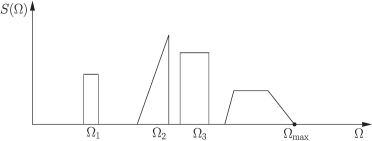
Figure 12: The Fourier transform of an analogue signal, $s(t)$, which is sparse in the frequency domain; only a limited number of frequency bands contribute to its spectrum content $S(\Omega)$, where $\Omega$ stands for the angular frequency. Nyquist’s theory guarantees that sampling at a frequency larger than or equal to twice the maximum $\Omega_{\max}$ is sufficient to recover the original analogue signal. However, this theory does not exploit information related to the sparse structure of the signal in the frequency domain.

An approach inspired directly by the theory of CS was first presented in [Kiro 06] and later improved and theoretically developed in [Trop 10]. The approach builds around the assumption that the signal consists of a sum of sinusoids and the random demodulator of Figure 11 is adopted. In [Mish 10, Mish 11b], the more general case of a signal consisting of a number of frequency bands, instead of tones, was treated. In addition, the task of extracting each band of the signal from the compressed measurements, that enables (low rate) baseband processing, is addressed. In principle, CS related theory would enable far fewer data samples than traditionally required when capturing signals with relatively high bandwidth, but with a low information rate. However, from a practical point of view, there are still a number of hardware implementation related issues, such as random jittering, to be solved first, e.g., [Chen 12, Maec 12].

An alternative path to sub-Nyquist sampling embraces a different class of analog signals known as multipulse signals; that is, signals that consist of a stream of short pulses. Sparsity now refers to the time domain, and such signals may not even be bandlimited. Signals of this type can be met in a number of applications, such as in radar, ultrasound, bioimaging and neuronal signal processing, see, e.g., [Drag 07]. An approach, known as finite rate of innovation sampling, passes an analogue signal, having $k$ degrees of freedom per second, through a linear time invariant filter and then samples at a rate of $2k$ samples per second. Reconstruction is performed via rooting a high-order polynomial, see, e.g., [Vett 02, Blu 08] and the references therein. In [Matu 12], the task of sub-Nyquist sampling is treated using CS theory arguments and an expansion in terms of Gabor functions; the signal is assumed to consist of a sum of a few pulses of finite duration, yet of unknown shape and time positions.

The task of sparsity-aware learning in the analogue domain is still in its early stages and there is currently a lot of on-going activity; more on this topic can be obtained in [Duar 11, Mish 11a] and the references there in.

11 Sparsity-Promoting Algorithms

In the previous sections, our emphasis was to highlight the most important aspects underlying the theory of sparse signal/vector recovery from an underdetermined set of linear equations. We now turn our attention to the algorithmic aspects of the problem [Elad 10]. The issue now becomes that of discussing efficient algorithmic schemes, which can achieve the recovery of the unknown set of parameters. In Sections 4 and 6, we saw that the constrained $\ell_{1}$ norm minimization (Basis Pursuit) can be solved via Linear Programming techniques and the LASSO task via convex optimization schemes. However, such general purpose techniques tend to be inefficient, since, often, they require many iterations to converge and the respective computational resources can be excessive for practical applications, especially in high dimensional spaces, $\mathcal{R}^{l}$. As a consequence, a huge research effort has been invested with the goal to develop efficient algorithms, that are tailored-made to these specific tasks. This is still a hot on-going area of research and definite conclusions are still risky to be drawn. Our aim here is to provide the reader with some general trends and philosophies that characterize the related activity. We will focus on the most commonly used and cited algorithms, which at the same time are structurally simple and the reader can follow them, without requiring a deeper knowledge on optimization. Moreover, these algorithms involve, in one way or another, arguments that are directly related to points and notions that we have already used while presenting the theory; thus, they can also be exploited from a pedagogical point of view, in order to strengthen the reader’s understanding of the topic. We start our review with the class of batch algorithms, where all data are assumed to be available prior to the application of the algorithm, and then we will move on to online/time-adaptive schemes. Furthermore, our emphasis is on algorithms that are appropriate for any sensing matrix. This is stated in order to point out that in the literature efficient algorithms have also been developed for specific forms of highly structured sensing matrices; exploiting their particular structure can lead to reduced computational demands, [Gilb 05, Need 09].

There are currently three rough types of families along which this algorithmic activity is growing: a) greedy algorithms, b) iterative shrinkage schemes, and c) convex optimization techniques. We have used the word rough, since, in some cases, it may be difficult to assign an algorithm to a specific family.

11.1 Greedy Algorithms

Greedy algorithms have a long history, see, for example, [Teml 03] for a comprehensive list of references. In the context of dictionary learning, a greedy algorithm known as Matching Pursuit was introduced in [Mall 93]. A greedy algorithm is built upon a series of locally optimal single-term updates. In our context, the goals are: a) to unveil the “active” columns of the sensing matrix $X$; that is, those columns that correspond to the nonzero locations of the unknown parameters and b) to estimate the respective sparse parameter vector. The set of indices which correspond to the nonzero vector components is also known as the support. To this end, the set of active columns of $X$ (and the support) is increased by one at each iteration step. In the sequel, an updated estimate of the unknown sparse vector is obtained. Let us assume that, at the $(i-1)$th iteration step, the algorithm has selected the columns denoted as $\mathbf{x}_{j_{1}},\mathbf{x}_{j_{2}},\ldots,\mathbf{x}_{j_{i-1}}$, with $j_{1},j_{2},\ldots,j_{i-1}\in\{1,2,\ldots,l\}$. These indices are the elements of the currently available support, $S^{(i-1)}$. Let $X^{(i-1)}$ be the $N\times(i-1)$ matrix having $\mathbf{x}_{j_{1}},\mathbf{x}_{j_{2}},\ldots,\mathbf{x}_{j_{i-1}}$ as its columns. Let, also, the current estimate of the solution be $\bm{\theta}^{(i-1)}$, which is a $(i-1)$-sparse vector, with zeros at all locations with index outside the support.

Algorithm 1 (Orthogonal Matching Pursuit (OMP)).

The algorithm is initialized with $\bm{\theta}^{(0)}\coloneqq\bm{0}$, $\bm{e}^{(0)}\coloneqq\bm{y}$ and $S^{(0)}\coloneqq\emptyset$. At iteration step $i$, the following computational steps are performed:

1. Select the column $\mathbf{x}_{j_{i}}$ of $X$, which is maximally correlated to (forms the least angle with) the respective error vector, $\bm{e}^{(i-1)}\coloneqq\bm{y}-X\bm{\theta}^{(i-1)}$, i.e.,

   $$\mathbf{x}_{j_{i}}:\ j_{i}\coloneqq\operatorname{arg\,max}_{j=1,2,\ldots,l}\frac{\left|\mathbf{x}_{j}^{T}\bm{e}^{(i-1)}\right|}{\left\|{\mathbf{x}_{j}}\right\|_{2}}.$$

2. Update the support and the corresponding set of active columns: $S^{(i)}=S^{(i-1)}\cup\{j_{i}\}$, and $X^{(i)}=[X^{(i-1)},\mathbf{x}_{j_{i}}]$.

3. Update the estimate of the parameter vector: Solve the Least-Squares (LS) problem that minimizes the norm of the error, using the active columns of $X$ only, i.e.,

   $$\tilde{\bm{\theta}}\coloneqq\operatorname{arg\,min}_{\bm{z}\in\mathcal{R}^{i}}\left\|{\bm{y}-X^{(i)}\bm{z}}\right\|_{2}^{2}.$$

   Obtain $\bm{\theta}^{(i)}$ by inserting the elements of $\tilde{\bm{\theta}}$ in the respective locations $(j_{1},j_{2},\ldots,j_{i})$, which comprise the support (the rest of the elements of $\bm{\theta}^{(i)}$ retain their zero values).

4. Update the error vector

   $$\bm{e}^{(i)}\coloneqq\bm{y}-X\bm{\theta}^{(i)}.$$

The algorithm terminates if the norm of the error becomes less than a preselected user-defined constant, $\epsilon_{0}$. The following observations are in order.

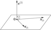
Figure 13: The error vector at the $i$th iteration is orthogonal to the subspace spanned by the currently available set of active columns. Here is an illustration for the case of the $3$-dimensional Euclidean space $\mathcal{R}^{3}$, and for $i=2$.

Remarks 10.

• Since $\bm{\theta}^{(i)}$, in Step 3, is the result of a LS task, it is known that the error vector is orthogonal to the subspace spanned by the active columns involved, i.e.,

  $$\bm{e}^{(i)}\bot\operatorname{span}\left\{\mathbf{x}_{j_{1}},\ldots,\mathbf{x}_{j_{i}}\right\}.$$

  This guarantees that taking the correlation, in the next step, of the columns of $X$ with $\bm{e}^{(i)}$ none of the previously selected columns will be reselected; they result to zero correlation, being orthogonal to $\bm{e}^{(i)}$, see Fig. 13.

• It can be shown that the column, which has maximal correlation (maximum absolute value of the inner product) with the currently available error vector, is the one that maximally reduces (compared to any other column) the $\ell_{2}$ norm of the error, when $\bm{y}$ is approximated by linearly combining the currently available active columns. This is the point where the heart of the greedy strategy beats. This minimization is with respect to a single term, keeping the rest fixed, as they have been obtained from the previous iteration steps [Bruc 09].

• Starting with all the components being zero, if the algorithm stops after $k_{0}$ iteration steps, the result will be a $k_{0}$-sparse solution.

• Note that there is no optimality in this searching strategy. The only guarantee is that the $\ell_{2}$ norm of the error vector is decreased at every iteration step. In general, there is no guarantee that the algorithm can obtain a solution close to the true one, see, e.g., [DeVo 96]. However, under certain constraints on the structure of $X$, performance bounds can be obtained, see, e.g., [Trop 04, Dave 10, Zhan 11].

• The complexity of the algorithm amounts to $\mathcal{O}(k_{0}lN)$ operations, which are contributed by the computations of the correlations, plus the demands raised by the solution of the LS task, in Step 3, whose complexity depends on the specific algorithm used. The $k_{0}$ is the sparsity level of the delivered solution and, hence, the total number of iteration steps that are performed.

Another more qualitative argument, that justifies the selection of the columns based on their correlation with the error vector, is the following. Assume that the matrix $X$ is orthonormal. Let also $\bm{y}=X\bm{\theta}$. Then, $\bm{y}$ lies in the subspace spanned by the active columns of X, i.e., those which correspond to the non-zero components of $\bm{\theta}$. Hence, the rest of the columns are orthogonal to $\bm{y}$, since $X$ is assumed to be orthonormal. Taking the correlation of $\bm{y}$, at the first iteration step, with all the columns, it is certain that one among the active columns will be chosen. The inactive columns result in zero correlation. A similar argument holds true for all subsequent steps, since all the activity takes place in a subspace that is orthogonal to all the inactive columns of $X$. In the more general case, where $X$ is not orthonormal, we can still use the correlation as a measure that quantifies geometric similarity. The smaller the correlation/the magnitude of the inner product is, the more orthogonal two vectors are. This brings us back to the notion of mutual coherence, which is a measure of the maximum correlation (least angle) among the columns of $X$.

11.1.1 OMP Can Recover Optimal Sparse Solutions: Sufficiency Condition

We have already stated that, in general, there are no guarantees that OMP will recover optimal solutions. However, when the unknown vector is sufficiently sparse, with respect to the structure of the sensing matrix $X$, then OMP can exactly solve the $\ell_{0}$ minimization task in (27) and recover the solution in $k_{0}$ steps, where $k_{0}$ is the sparsest solution that satisfies the associated linear set of equations.

Theorem 5.

Let the mutual coherence (Section 7.1) of the sensing matrix, $X$, be $\mu(X)$. Assume, also, that the linear system, $\bm{y}=X\bm{\theta}$, accepts a solution such as

$$\left\|{\bm{\theta}}\right\|_{0}<\frac{1}{2}\left(1+\frac{1}{\mu(X)}\right).$$ (47)

Then, OMP guarantees to recover the sparsest solution in $k_{0}=\left\|{\bm{\theta}}\right\|_{0}$ steps.

We know from Section 7.1 that, under the previous condition, any other solution will be necessarily less sparse. Hence, there is a unique way to represent $\bm{y}$ in terms of $k_{0}$ columns of $X$. Without harming generality, let us assume that the true support corresponds to the first $k_{0}$ columns of $X$, i.e.,

$$\bm{y}=\sum_{j=1}^{k_{0}}\theta_{j}\mathbf{x}_{j},\quad\theta_{j}\neq 0,\forall j\in\{1,\ldots,k_{0}\}.$$

The theorem is a direct consequence of the following proposition:

Proposition 1.

If the condition (47) holds true, then the OMP algorithm will never select a column with index outside the true support, see, e.g., [Trop 04]. In a more formal way, this is expressed as

$$j_{i}=\operatorname{arg\,max}_{j=1,2,\ldots,l}\frac{\left|\mathbf{x}_{j}^{T}\bm{e}^{(i-1)}\right|}{\left\|{\mathbf{x}_{j}}\right\|_{2}}\in\{1,\ldots,k_{0}\}.$$

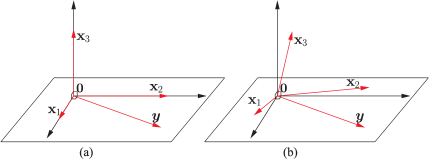
Figure 14: (a) In the case of an orthogonal matrix, the measurement vector $\bm{y}$ will be orthogonal to any inactive column; here, $\mathbf{x}_{3}$. (b) In the more general case, it is expected to “lean” closer (form smaller angles) to the active than to the inactive columns.

A geometric interpretation of this proposition is the following: if the angles formed between all the possible pairs among the columns of $X$ are large enough in the $\mathcal{R}^{l}$ space, which guarantees that $\mu(X)$ is small enough, then $\bm{y}$ will lean more (form smaller angle) towards any one of the active columns, which contribute to its formation, compared to the rest, which are inactive and do not participate in the linear combination that generates $\bm{y}$. Fig. 14 illustrates the geometry, for the extreme case of mutually orthogonal vectors (Fig. 14a) and for the more general case, where the vectors are not orthogonal, yet the angle between any pair of columns is large enough (Fig. 14b).

In a nutshell, the previous proposition guarantees that, during the first iteration, a column corresponding to the true support will be selected. In a similar way, this is also true for all subsequent iterations. In the second step, another, different from the previously selected column (as it has already been stated), will be chosen. At step $k_{0}$, the last remaining active column, corresponding to the true support, is selected and this necessarily results to zero error. To this end, it suffices to set $\epsilon_{0}$ equal to zero.

11.1.2 The LARS Algorithm

The Least Angle Regression (LARS) algorithm, [Efro 04], shares the first two steps with OMP. It selects $j_{i}$ to be an index outside the currently available active set so that to maximize the correlation with the residual vector. However, instead of performing an LS fit to compute the nonzero components of $\bm{\theta}^{(i)}$, these are computed so that the residual to be equicorrelated with all the columns in the active set, i.e.,

$$|\mathbf{x}_{j}^{T}(\bm{y}-X\bm{\theta}^{(i)})|=\text{constant},\quad\forall j\in S^{(i)},$$

where we have assumed that the columns of $X$ are normalized, as it is common in practice (recall, also, the Remarks 4). In other words, in contrast to the OMP, where the error vector is forced to be orthogonal to the active columns, LARS demands this error to form equal angles with each one of them. Likewise OMP, it can be shown that, provided the target vector is sufficiently sparse and under incoherence of the columns of $X$, LARS can exactly recover the sparsest solution, [Tsai 07].

A further small modification leads to the so-called LARS-LASSO algorithm. According to this version, a previously selected index in the active set can be removed at a later stage. This gives the algorithm the potential to “recover” from a previously bad decision. Hence, this modification departs from the strict rationale that defines the greedy algorithms. It turns out that this version solves the LASSO optimization task. This algorithm is the same as the one suggested in [Osbo 00] and it is known as homotopy algorithm. Homotopy methods are based on a continuous transformation from one optimization task to another. The solutions to this sequence of tasks lie along a continuous parameterized path. The idea is that, while the optimization tasks may be difficult to solve by themselves, one can trace this path of solutions by slowly varying the parameters. For the LASSO task, it is the $\lambda$ parameter which is varying, see, e.g., [Plum 05, Mali 05, Asif 10a]. Take as an example the LASSO task in its regularized version in (13). For $\lambda=0$, the task minimizes the $\ell_{2}$ norm and for $\lambda\rightarrow\infty$ the task minimizes the $\ell_{1}$ norm, and for this case the solution tends to zero. It turns out that the solution path, as $\lambda$ changes from large to small values, is polygonal. Vertices on this solution path correspond to vectors having nonzero elements only on a subset of entries. This subset remains unchanged, till $\lambda$ reaches the next critical value, which corresponds to a new vertex of the polygonal path and to a new subset of potential nonzero values. Thus, the solution is obtained via this sequence of steps along this polygonal path.

11.1.3 Compressed Sensing Matching Pursuit (CSMP) Algorithms

Strictly speaking, these algorithms are not greedy, yet, as it is stated in [Need 09], they are at heart greedy algorithms. Instead of performing a single term optimization per iteration step, in order to increase the support by one, as it is the case with OMP, these algorithms attempt to obtain first an estimate of the support and then use this information to compute a least squares estimate of the target vector, constrained on the respective active columns. The quintessence of the method lies in the near-orthogonal nature of the sensing matrix, assuming that this obeys the RIP.

Assume that $X$ obeys the RIP for some small enough value $\delta_{k}$ and sparsity level, $k$, of the unknown vector. Let, also, that the measurements are exact, i.e., $\bm{y}=X\bm{\theta}$. Then, $X^{T}\bm{y}=X^{T}X\bm{\theta}\approx\bm{\theta}$. Therefore, intuition indicates that it is not unreasonable to select, in the first iteration step, the $t$ (a user-defined parameter) largest in magnitude components of $X^{T}\bm{y}$ as indicative of the nonzero positions of the sparse target vector. This reasoning carries on for all subsequent steps, where, at the $i$th iteration, the place of $\bm{y}$ is taken by the residual $\bm{e}^{(i-1)}\coloneqq\bm{y}-X\bm{\theta}^{(i-1)}$, where $\bm{\theta}^{(i-1)}$ indicates the estimate of the target vector at the $(i-1)$th iteration. Basically, this could be considered as a generalization of the OMP. However, as we will soon see, the difference between the two mechanisms is more substantial.

Algorithm 2 (The CSMP Scheme).

1. Select the value of $t$.

2. Initialize the algorithm: $\bm{\theta}^{(0)}=\bm{0}$, $\bm{e}^{(0)}=\bm{y}$.

3. For $i=1,2,\ldots$, execute the following.

   1. Obtain the current support:

      $$S^{(i)}\coloneqq\operatorname{supp}\left(\bm{\theta}^{(i-1)}\right)\cup\left\{\text{indices of the}\ t\ \text{largest in magnitude}\atop\text{components of}\ X^{T}\bm{e}^{(i-1)}\right\}.$$

   2. Select the active columns: Construct $X^{(i)}$ to comprise the active columns of $X$ in accordance to $S^{(i)}$. Obviously, $X^{(i)}$ is a $N\times r$ matrix, where $r$ denotes the cardinality of the support set $S^{(i)}$.

   3. Update the estimate of the parameter vector: solve the LS task

      $$\tilde{\bm{\theta}}\coloneqq\operatorname{arg\,max}_{\bm{z}\in\mathcal{R}^{r}}\left\|{\bm{y}-X^{(i)}\bm{z}}\right\|_{2}^{2}.$$

      Obtain $\hat{\bm{\theta}}^{(i)}\in\mathcal{R}^{l}$ having the $r$ elements of $\tilde{\bm{\theta}}$ in the respective locations, as indicated by the support, and the rest of the elements being zero.

   4. $\bm{\theta}^{(i)}\coloneqq H_{k}\left(\hat{\bm{\theta}}^{(i)}\right)$. The mapping $H_{k}$ denotes the hard thresholding operator; that is, it returns a vector with the $k$ largest in magnitude components of the argument, and the rest are forced to zero.

   5. Update the error vector: $\bm{e}^{(i)}=\bm{y}-X\bm{\theta}^{(i)}$.

The algorithm requires as input the sparsity level $k$. Iterations carry on until a halting criterion is met. The value of $t$, that determines the largest in magnitude values in Steps 1 and 3a, depends on the specific algorithm. In CoSaMP (Compressive Sampling Matching Pursuit, [Need 09]), $t=2k$ and in the SP (Subspace Pursuit, [Dai 09]), $t=k$.

Having stated the general scheme, a major difference with OMP becomes readily apparent. In OMP, only one column is selected per iteration step. Moreover, this remains in the active set for all subsequent steps. If, for some reason, this was not a good choice, the scheme cannot recover from such a bad decision. In contrast, the support and hence the active columns of $X$ are continuously updated in CSMP and the algorithm has the ability to correct a previously bad decision, as more information is accumulated and iterations progress. In [Dai 09], it is shown that if the measurements are exact ($\bm{y}=X\bm{\theta}$) then SP can recover the $k$-sparse true vector in a finite number of iteration steps, provided that $X$ satisfies the RIP with $\delta_{3k}<0.205$. If the measurements are noisy, performance bounds have been derived, which hold true for $\delta_{3k}<0.083$. For the CoSaMP, performance bounds have been derived for $\delta_{4k}<0.1$.

11.2 Iterative Shrinkage Algorithms (IST)

This family of algorithms have also a long history, see, e.g., [Jans 84, Dono 94, Hoch 90, King 02]. However, in the “early” days, the developed algorithms had some sense of heuristic flavor, without establishing a clear bridge with optimizing a cost function. Later attempts were substantiated by sound theoretical arguments concerning issues such as convergence and convergence rate, e.g., [Figu 03, Daub 04, Elad 07a, Comb 05].

The general form of this algorithmic family has a striking resemblance with the classical linear algebra iterative schemes for approximating the solution of large linear systems of equations, known as stationary iterative or iterative relaxation methods. The classical Gauss-Seidel and Jacobi algorithms, e.g., [Hage 81], in numerical analysis can be considered as members of this family. Given a linear system of $l$ equations with $l$ unknowns, $\bm{z}=A\bm{x}$, the basic iteration at step $i$ has the following form

$$\bm{x}^{(i)} = \left(I-QA\right)\bm{x}^{(i-1)}+Q\bm{z}$$

$$= \bm{x}^{(i-1)}+Q\bm{e}^{(i-1)},\qquad\bm{e}^{(i-1)}\coloneqq\bm{z}-A\bm{x}^{(i-1)},$$

which does not come as a surprise. It is of the same form as most of the iterative schemes for numerical solutions! The matrix $Q$ is chosen so that to guarantee convergence and different choices lead to different algorithms with their pros and cons. It turns out that this algorithmic form can also be applied to underdetermined systems of equations, $\bm{y}=X\bm{\theta}$, with a “minor” modification, which is imposed by the sparsity constraint of the target vector. This leads to the following general form of iterative computation

$$\bm{\theta}^{(i)}=T_{i}\left(\bm{\theta}^{(i-1)}+Q\bm{e}^{(i-1)}\right),\qquad\bm{e}^{(i-1)}=\bm{y}-X\bm{\theta}^{(i-1)},$$

starting from an initial guess of $\bm{\theta}^{(0)}$ (usually $\bm{\theta}^{(0)}=\bm{0}$, $\bm{e}^{(0)}=\bm{y}$). In certain cases, $Q$ can be made to be iteration-dependent. The operator $T_{i}(\cdot)$ is a nonlinear thresholding operator, that is applied entrywise, i.e., component-wise. Depending on the specific scheme, this can be either the hard thresholding operator, denoted as $H_{k}$, or the soft thresholding operator, denoted as $S_{\alpha}$. Hard thresholding, as we already know, keeps the $k$ largest components of a vector unaltered and sets the rest equal to zero. Soft thresholding was introduced in Section 4. All components with magnitude less than $\alpha$ are forced to zero and the rest are reduced in magnitude by $\alpha$; that is, the $j$th component of a vector, $\bm{\theta}$, after soft thresholding becomes

$$(S_{\alpha}(\bm{\theta}))_{j}=\operatorname{sgn}(\theta_{j})(|\theta_{j}|-\alpha)_{+}.$$

Depending on a) the choice of $T_{i}$, b) the specific value of the parameter $k$ or $\alpha$ and c) the matrix $Q$, different instances occur. A most common choice for $Q$ is $\mu X^{T}$ and the generic form of the main iteration becomes

$$\bm{\theta}^{(i)}=T_{i}\left(\bm{\theta}^{(i-1)}+\mu X^{T}\bm{e}^{(i-1)}\right),$$ (48)

where $\mu$ is a relaxation (user-defined) parameter, which can also be left to vary with each iteration step. The choice of $X^{T}$ is intuitively justified, once more, by the near-orthogonal nature of $X$. For the first iteration step and for a linear system of the form $\bm{y}=X\bm{\theta}$, starting from a zero initial guess, we have $X^{T}\bm{y}=X^{T}X\bm{\theta}\approx\bm{\theta}$ and we are close to the solution.

Although intuition is most important in scientific research, it is not enough, by itself, to justify decisions and actions. The generic scheme in (48) has been reached from different paths, following different perspectives that lead to different choices of the respective parameters. Let us spend some more time on that, with the aim to make the reader more familiar with techniques that address optimization tasks of non-differentiable loss functions. The term in the parenthesis in (48) coincides with the gradient descent iteration step if the cost function were the unregularized LS loss, i.e.,

$$J(\bm{\theta})=\frac{1}{2}\left\|{\bm{y}-X\bm{\theta}}\right\|_{2}^{2}.$$

In this case, the gradient descent rationale leads to

$$\bm{\theta}^{(i-1)}-\mu\frac{\partial J\left(\bm{\theta}^{(i-1)}\right)}{\partial\bm{\theta}} =\bm{\theta}^{(i-1)}-\mu X^{T}(X\bm{\theta}^{(i-1)}-\bm{y})$$

$$=\bm{\theta}^{(i-1)}+\mu X^{T}\bm{e}^{(i-1)}.$$

It is well known and it can easily be shown that the gradient descent can alternatively be viewed as the result of minimizing a regularized version of the linearized loss function, i.e.,

$$\bm{\theta}^{(i)}=\operatorname{arg\,min}_{\bm{\theta}\in\mathcal{R}^{l}}\left\{J\left(\bm{\theta}^{(i-1)}\right)\right. +\left(\bm{\theta}-\bm{\theta}^{(i-1)}\right)^{T}\frac{\partial J\left(\bm{\theta}^{(i-1)}\right)}{\partial\bm{\theta}}$$

$$+\left.\frac{1}{2\mu}\left\|{\bm{\theta}-\bm{\theta}^{(i-1)}}\right\|^{2}_{2}\right\}.$$ (49)

One can adopt this view of the gradient descent philosophy as a kick-off point to minimize iteratively the following LASSO task, i.e.,

$$\min_{\bm{\theta}\in\mathcal{R}^{l}}\left\{L(\bm{\theta},\lambda)=\frac{1}{2}\left\|{\bm{y}-X\bm{\theta}}\right\|_{2}^{2}+\lambda\left\|{\bm{\theta}}\right\|_{1}=J(\bm{\theta})+\lambda\left\|{\bm{\theta}}\right\|_{1}\right\}.$$

The difference now is that the loss function comprises two terms. One which is smooth (differentiable) and a non-smooth one. Let the current estimate be $\bm{\theta}^{(i-1)}$. The updated estimate is obtained by

$$\bm{\theta}^{(i)}=\operatorname{arg\,min}_{\bm{\theta}\in\mathcal{R}^{l}}\left\{J\left(\bm{\theta}^{(i-1)}\right)\right. +\left(\bm{\theta}-\bm{\theta}^{(i-1)}\right)^{T}\frac{\partial J(\bm{\theta}^{(i-1)})}{\partial\bm{\theta}}$$

$$+\left.\frac{1}{2\mu}\left\|{\bm{\theta}-\bm{\theta}^{(i-1)}}\right\|^{2}_{2}+\lambda\left\|{\bm{\theta}}\right\|_{1}\right\},$$

which, after ignoring constants, becomes

$$\bm{\theta}^{(i)}=\operatorname{arg\,min}_{\bm{\theta}\in\mathcal{R}^{l}}\left\{\frac{1}{2}\left\|{\bm{\theta}-\tilde{\bm{\theta}}}\right\|^{2}_{2}+\lambda\mu\left\|{\bm{\theta}}\right\|_{1}\right\}$$ (50)

where

$$\tilde{\bm{\theta}}:=\bm{\theta}^{(i-1)}-\mu\frac{\partial J(\bm{\theta}^{(i-1)})}{\partial\bm{\theta}}.$$ (51)

Following exactly the same steps as those that led to the derivation of (20) from (13) (after replacing $\hat{\bm{\theta}}_{LS}$ with $\tilde{\bm{\theta}}$) we obtain

$$\bm{\theta}^{(i)} = S_{\lambda\mu}(\tilde{\bm{\theta}})=S_{\lambda\mu}\left(\bm{\theta}^{(i-1)}-\mu\frac{\partial J(\bm{\theta}^{(i-1)})}{\partial\bm{\theta}}\right)$$ (52)

$$= S_{\lambda\mu}\left(\bm{\theta}^{(i-1)}+\mu X^{T}\bm{e}^{(i-1)}\right).$$ (53)

This is very interesting and practically useful. The only effect of the presence of the non-smooth $\ell_{1}$ norm in the loss function is an extra simple thresholding operation, which as we know is an operation performed individually on each component. It can be shown, e.g., [Beck 09], that this algorithm converges to a minimizer $\bm{\theta}_{*}$ of the LASSO (13), provided that $\mu\in(0,1/\lambda_{\max}(X^{T}X))$, where $\lambda_{\max}(\cdot)$ denotes the maximum eigenvalue of $X^{T}X$. The convergence rate is dictated by the rule

$$L(\bm{\theta}^{(i)},\lambda)-L(\bm{\theta}_{*},\lambda)\approx O(1/i),$$

which is known as sublinear global rate of convergence. Moreover, it can be shown that

$$L(\bm{\theta}^{(i)},\lambda)-L(\bm{\theta}_{*},\lambda)\leq\frac{C\left\|{\bm{\theta}^{(0)}-\bm{\theta}_{*}}\right\|^{2}_{2}}{2i}.$$

The latter result indicates that if one wants to achieve an accuracy of $\epsilon$, then this can be obtained by at most $\left\lfloor\frac{C\left\|{\bm{\theta}^{(0)}-\bm{\theta}_{*}}\right\|^{2}_{2}}{2\epsilon}\right\rfloor$ iterations, where $\lfloor\cdot\rfloor$ denotes the floor operator.

In [Daub 04], (48) was obtained from a nearby corner, building upon arguments from the classical proximal-point methods in optimization theory, e.g., [Rock 76]. The original LASSO regularized cost function is modified to the so called surrogate objective,

$$J(\bm{\theta},\tilde{\bm{\theta}})=\frac{1}{2}\left\|{\bm{y}-X\bm{\theta}}\right\|_{2}^{2}+\lambda\left\|{\bm{\theta}}\right\|_{1}+\frac{1}{2}d(\bm{\theta},\tilde{\bm{\theta}}),$$

where

$$d(\bm{\theta},\tilde{\bm{\theta}})\coloneqq c\left\|{\bm{\theta}-\tilde{\bm{\theta}}}\right\|_{2}^{2}-\left\|{X\bm{\theta}-X\tilde{\bm{\theta}}}\right\|^{2}_{2}.$$

If $c$ is appropriately chosen (larger than the largest eigenvalue of $X^{T}X$), the surrogate objective is guaranteed to be strictly convex. Then it can be shown that the minimizer of the surrogate objective is given by

$$\hat{\bm{\theta}}=S_{\lambda/c}\left(\tilde{\bm{\theta}}+\frac{1}{c}X^{T}(\bm{y}-X\tilde{\bm{\theta}})\right).$$ (54)

In the iterative formulation, $\tilde{\bm{\theta}}$ is selected to be the previously obtained estimate; in this way, one tries to keep the new estimate close to the previous one. The procedure readily results to our generic scheme in (48), using soft thresholding with parameter $\lambda/c$. It can be shown that such a strategy converges to a minimizer of the original LASSO problem. The same algorithm was reached in [Figu 03], using majorization-minimization techniques from optimization theory. So, from this perspective, the IST family has strong ties with algorithms that belong to the convex optimization category.

In [Wrig 09b], the Sparse Reconstruction by Separable Approximation (SpaRSA) algorithm is proposed, which is a modification of the standard IST scheme. The starting point is (49); however, the multiplying factor, $\frac{1}{2\mu}$, instead of being constant is now allowed to change from iteration to iteration according to a rule. This results in a speed up in the convergence of the algorithm. Moreover, inspired by the homotopy family of algorithms, where $\lambda$ is allowed to vary, SpaRSA can be extended to solve a sequence of problems which are associated with a corresponding sequence of values of $\lambda$. Once a solution has been obtained for a particular value of $\lambda$, it can be used as a “warm-start” for a nearby value. Solutions can therefore be computed for a range of values, at a small extra computational cost, compared to solving for a single value from a “cold start”. This technique abides with to the so-called continuation strategy, which has been used in the context of other algorithms as well, e.g., [Hale 07]. Continuation has been shown to be a very successful tool to increase the speed of convergence.

An interesting modification of the basic IST scheme has been proposed in [Beck 09], which improves the convergence rate to $O(1/i^{2})$, by only a simple modification with almost no extra computational burden. The scheme is known as Fast Iterative Shrinkage-Thresholding Algorithm (FISTA). This scheme is an evolution of [Nest 83], which introduced the basic idea for the case of differentiable costs, and consists of the following steps:

$$\bm{\theta}^{(i)} = S_{\lambda\mu}\left(\bm{z}^{(i)}+\mu X^{T}\left(\bm{y}-X\bm{z}^{(i)}\right)\right),$$

$$\bm{z}^{(i+1)} \coloneqq \bm{\theta}^{(i)}+\frac{t_{i}-1}{t_{i+1}}\left(\bm{\theta}^{(i)}-\bm{\theta}^{(i-1)}\right),$$

where

$$t_{i+1}\coloneqq\frac{1+\sqrt{1+4t^{2}_{i}}}{2},$$

with initial points $t_{1}=1$ and $\bm{z}^{(1)}=\bm{\theta}^{(0)}$. In words, in the thresholding operation, $\bm{\theta}^{(i-1)}$ is replaced by $\bm{z}^{(i)}$, which is a specific linear combination of two successive updates of $\bm{\theta}$. Hence, at a marginal increase of the computational cost, a substantial increase in convergence speed is achieved.

In [Blum 09a] the hard thresholding version has been used, with $\mu=1$ and the thresholding operator $H_{k}$ uses the sparsity level $k$ of the target solution, that is assumed to be known. In a later version, [Blum 10], the relaxation parameter is left to change so that, at each iterations step, the error is maximally reduced. It has been shown that the algorithm converges to a local minimum of the cost function $\left\|{\bm{y}-X\bm{\theta}}\right\|_{2}$, under the constraint that $\bm{\theta}$ is a $k$-sparse vector. Moreover, the latter version is a stable one and it results to a near optimal solution if a form of RIP is fulfilled.

A modified version of the generic scheme given in (48), that evolves along the lines of [Luo 92], obtains the updates component-wise, one vector component at a time. Thus, a “full” iteration consists of $l$ steps. The algorithm is known as coordinate descent and its basic iteration has the form,

$$\theta_{j}^{(i)}=S_{\lambda/\left\|{\mathbf{x}_{j}}\right\|_{2}^{2}}\left(\theta^{(i-1)}_{j}+\frac{{\mathbf{x}_{j}^{T}\bm{e}^{(i-1)}}}{\left\|{\mathbf{x}_{j}}\right\|^{2}_{2}}\right),\quad j=1,2,\ldots,l.$$ (55)

This algorithm replaces the constant $c$, in the previously reported soft thresholding algorithm, with the norm of the respective column of $X$, if the columns of $X$ are not normalized to unit norm. It has been shown that the parallel coordinate descent algorithm also converges to a LASSO minimizer of (13), [Elad 07a]. Improvements of the algorithm, using line search techniques to determine the most descent direction for each iteration, have also been proposed, see, [Zibu 10].

The main contribution to the complexity for the iterative shrinkage algorithmic family comes from the two matrix-vector products, which amounts to $\mathcal{O}(Nl)$, unless $X$ has a special structure, e.g., DFT, that can be exploited to reduce the load.

In [Male 10], the so-called Two Stage Thresholding (TST) scheme is presented, which brings together arguments from the iterative shrinkage family and the OMP. This algorithmic scheme involves two stages of thresholding. The first step is exactly the same as in (48). However, this is now used only for determining “significant” nonzero locations, just as in Compressed Sensing Matching Pursuit (CSMP) algorithms, presented in the previous subsection. Then, a LS problem is solved to provide the updated estimate, under the constraint of the available support. This is followed by a second step of thresholding. The thresholding operations in the two stages can be different. If hard thresholding, $H_{k}$, is used in both steps, this results to the algorithm proposed in [Fouc 11]. For this latter scheme, convergence and performance bounds are derived if the RIP holds for $\delta_{3k}<0.58$. In other words, the basic difference between the TST and CSMP approaches is that, in the latter case, the most significant non-zero coefficients are obtained by looking at the correlation term $X^{T}\bm{e}^{(i-1)}$ and in the TST family at $\bm{\theta}^{(i-1)}+\mu X^{T}\bm{e}^{(i-1)}$. The differences among different approaches can be minor and the crossing lines among the different algorithmic categories are not necessarily crispy clear. However, from a practical point of view, sometimes small differences may lead to substantially improved performance.

Remarks 11.

• The minimization in (52) bridges the IST algorithmic family with another powerful tool in convex optimization, which builds around the notion of proximal mapping or Moreau envelopes, see, e.g., [Rock 76, Comb 11]. Given a convex function $h:\mathcal{R}^{l}\rightarrow\mathcal{R}$, and a $\mu>0$, the proximal mapping, $\operatorname{Prox}_{\mu h}:\mathcal{R}^{l}\rightarrow\mathcal{R}^{l}$, with respect to $h$, and of index $\mu$, is defined as the (unique) minimizer

  $$\operatorname{Prox}_{\mu h}(\bm{x})\coloneqq\operatorname{arg\,min}_{\bm{u}\in\mathcal{R}^{l}}\left\{h(\bm{u})+\frac{1}{2\mu}\left\|{\bm{x}-\bm{u}}\right\|_{2}^{2}\right\},\quad\forall\bm{x}\in\mathcal{R}^{l}.$$ (56)

  Let us now assume that we want to minimize a convex function, which is given as the sum

  $$f(\bm{\theta})=J(\bm{\theta})+h(\bm{\theta}),$$

  where $J(\cdot)$ is convex and differentiable, and $h(\cdot)$ is also a convex, but not necessarily a smooth one. Then it can be shown that the following iterations converge to a minimizer of $f(\cdot)$,

  $$\bm{\theta}^{(i)}=\operatorname{Prox}_{\mu h}\left(\bm{\theta}^{(i-1)}-\mu\frac{\partial J(\bm{\theta}^{(i-1)})}{\partial\bm{\theta}}\right),$$ (57)

  where $\mu>0$ and it can also be made iteration dependent, i.e., $\mu_{i}>0$. If we now use this scheme to minimize our familiar cost, i.e.,

  $$J(\bm{\theta})+\lambda\left\|{\bm{\theta}}\right\|_{1},$$

  we obtain (52); this is so, because the proximal operator of $h(\bm{\theta}):=\lambda\left\|{\bm{\theta}}\right\|_{1}$ is shown ([Comb 11, Comb 05]) to be identical to the soft thresholding operator, i.e.,

  $$\operatorname{Prox}_{h}(\bm{\theta})=S_{\lambda}(\bm{\theta}).$$

  In order to feel more comfortable with this operator, note that if $h(\bm{x}):=0$, its proximal operator is equal to $\bm{x}$, and in this case (57) becomes our familiar gradient descent algorithm.

• All the non-greedy algorithms, which have been discussed so far, have been developed to solve the task defined in the formulation (13). This is mainly because this is an easier task to solve; once $\lambda$ has been fixed, it is an unconstrained optimization task. However, there are algorithms which have been developed to solve the alternative formulations.

  The NESTA algorithm has been proposed in [Beck 11] and solves the task in its (15) formulation. Adopting this path can have an advantage since $\epsilon$ may be given as an estimate of the uncertainty associated with the noise, which can readily be obtained in a number of practical applications. In contrast, selecting a-priori the value for $\lambda$ is more intricate. In [Chen 98], the value $\lambda=\sigma_{\eta}\sqrt{2\ln l}$, where $\sigma_{\eta}$ is the noise standard deviation, is argued to have certain optimality properties; however this argument hinges on the assumption of the orthogonality of $X$. NESTA relies heavily on Nesterov’s generic scheme ([Nest 83]), hence its name. The original Nesterov’s algorithm performs a constrained minimization of a smooth convex function $f(\bm{\theta})$, i.e.,

  $$\min_{\bm{\theta}\in Q}f(\bm{\theta})$$

  where $Q$ is a convex set, and in our case this is associated with the quadratic constraint in (15). The algorithm consists of three basic steps. The first one is similar with the step in (49), i.e

  $$\bm{w}^{(i)}=\operatorname{arg\,min}_{\bm{\theta}\in Q}\left\{\left(\bm{\theta}-\bm{\theta}^{(i-1)}\right)^{T}\frac{\partial J\left(\bm{\theta}^{(i-1)}\right)}{\partial\bm{\theta}}+\frac{L}{2}\left\|{\bm{\theta}-\bm{\theta}^{(i-1)}}\right\|^{2}_{2}\right\},$$ (58)

  where $L$ is an upper bound on the Lipschitz coefficient, which the gradient of $f(\cdot)$ has to satisfy. The difference with (49) is that the minimization is now a constrained one. However, Nesterov has also added a second step involving another auxiliary variable, $\bm{z}^{(i)}$, which is computed in a similar way as $\bm{w}^{(i)}$ but the linearised term is now replaced by a weighted cumulative gradient,

  $$\sum_{k=0}^{i-1}\alpha_{k}\left(\bm{\theta}-\bm{\theta}^{(k)}\right)^{T}\frac{\partial J\left(\bm{\theta}^{(k)}\right)}{\partial\bm{\theta}}.$$

  The effect of this term is to smooth out the “zig-zagging” of the path towards the solution, whose effect is to increase significantly the convergence speed. The final step of the scheme involves an averaging of the previously obtained variables,

  $$\bm{\theta}^{(i)}=t_{i}\bm{z}^{(i)}+(1-t_{i})\bm{w}^{(i)}.$$

  The values of the parameters $\alpha_{k}$, $k=0,\ldots,i-1$, and $t_{i}$ result from the theory so that convergence is guaranteed. As it was the case with its close relative FISTA, the algorithm enjoys an $O(1/i^{2})$ convergence rate. In our case, where the function to be minimized, $\left\|{\bm{\theta}}\right\|_{1}$, is not smooth, NESTA uses a smoothed prox-function of it. Moreover, it turns out that close-form updates are obtained for $\bm{z}^{(i)}$ and $\bm{w}^{(i)}$. If $X$ is chosen so that to have orthonormal rows, the complexity per iteration is $O(l)$ plus the computations needed for performing the product $X^{T}X$, which is the most computational thirsty part. However, this complexity can substantially be reduced if the sensing matrix is chosen to be a submatrix of a unitary transform, which admits fast matrix-vector product computations, e.g., a subsampled DFT matrix. For example, for the case of a subsampled DFT matrix, the complexity amounts to $O(l)$ plus the load to perform the two Fast Fourier Transforms (FFT). Moreover, the continuation strategy can also be employed to accelerate convergence. In [Beck 11], it is demonstrated that NESTA exhibits good accuracy results, while retaining a complexity that is competitive with algorithms developed around the (15) formulation and scales in an affordable way for large size problems. Furthermore, NESTA, and in general Nesterov’s scheme, enjoy a generality that allows their use to other optimization tasks as well.

• The task in (14) has been considered in [Berg 08] and [Osbo 00]. In the former, the algorithm comprises a projection on the $l_{1}$ ball $\left\|{\bm{\theta}}\right\|_{1}\leq\rho$ (see also, Section 13.4) per iteration step. The most computationally dominant part of the algorithm consists of matrix-vector products. In [Osbo 00], a homotopy algorithm is derived for the same task, where now the bound $\rho$ becomes the homotopy parameter which is left to vary. This algorithm is also referred as the LARS-LASSO, as it has already been reported before.

11.3 Which Algorithm Then: Some Practical Hints

We have already discussed a number of algorithmic alternatives to obtain solutions to the $\ell_{0}/\ell_{1}$ norm minimization task. Our focus was on schemes whose computational demands are rather low and they scale well to very large problem sizes. We have not touched more expensive methods such as interior point methods for solving the $\ell_{1}$ convex optimization task. A review of such methods is provided in [Kim 07]. Interior point methods evolve along the Newton-type recursion and their complexity per iteration step is at least of the order $\mathcal{O}(l^{3})$. As it is most often the case, there is a trade off. Schemes of higher complexity tend to result in enhanced performance. However, such schemes become impractical in problems of large size. Some examples of other algorithms, that were not discussed, can be found in [Yin 08, Berg 08, Daub 10, Wrig 09b]. Talking about complexity, it has to be pointed out that what really matters at the end is not so much the complexity per iteration step but the overall required resources in computer time/memory for the algorithm to converge to a solution within a specified accuracy. For example, an algorithm may be of low complexity per iteration step but it may need an excessive number of iterations to converge.

Computational load is only one among a number of indices that characterize the performance of an algorithm. Other performance measures, refer to convergence rate, tracking speed (for the adaptive algorithms), and stability with respect to the presence of noise and/or finite word length computations. No doubt, all these performance measures are also of interest here, too. However, there is an additional aspect that is of particular importance when quantifying performance of sparsity-promoting algorithms. This is related to the so called undersampling-sparsity tradeoff or the phase transition curve.

One of the major issues, on which we focused in this paper, was to derive and present the conditions that guarantee uniqueness of the $\ell_{0}$ minimization and its equivalence with the $\ell_{1}$ minimization task, under an underdetermined set of measurements, $\bm{y}=X\bm{\theta}$, for the recovery of sparse enough signals/vectors. While discussing the various algorithms in this section, we reported a number of different RIP-related conditions that some of the algorithms have to satisfy in order to recover the target sparse vector. As a matter of fact, it has to be admitted that this was quite confusing, since each algorithm had to satisfy its own conditions. In addition, in practice, these conditions are not easy to be verified. Although such results are, no doubt, important to establish convergence and make us more confident and also understand better why and how an algorithm works, one needs further experimental evidence in order to establish good performance bounds for an algorithm. Moreover, all the conditions that we have dealt with, including coherence and RIP, are sufficient conditions. In practice, it turns out that sparse signal recovery is possible with sparsity levels much higher than those predicted by the theory, for given $N$ and $l$. Hence, proposing a new algorithm or selecting an algorithm from an available palette, one has to demonstrate experimentally the range of sparsity levels that can be recovered by the algorithm, as a percentage of the number of measurements and the dimensionality. Thus, in order to select an algorithm, one should cast his/her vote for the algorithm which, for given $l$ and $N$, has the potential to recover $k$-sparse vectors with $k$ being as high as possible, for most of the cases, that is, with high probability.

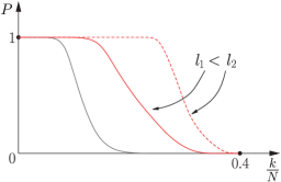
Figure 15: For any algorithm, the transition between the regions of 100% success and of a complete failure is very sharp. For the algorithm corresponding to the red curve, this transition occurs at higher sparsity values and, from this point of view, it is a better algorithm than the one associated with the black curve. Also, given a algorithm, the higher the dimensionality the higher the sparsity level where this transition occurs, as indicated by the two red curves.

Fig. 15 illustrates the type of curve that is expected to result in practice. The vertical axis is the probability of exact recovery of a target $k$-sparse vector and the horizontal axis shows the ratio $k/N$, for a given number of measurements, $N$, and the dimensionality of the ambient space, $l$. Three curves are shown. The red ones correspond to the same algorithm, for two different values of the dimensionality, $l$, and the gray one corresponds to another algorithm. Curves of this shape are expected to result from experiments of the following set up. Assume that we are given a sparse vector, $\bm{\theta}_{0}$, with $k$ nonzero components in the $l$-dimensional space. Using a sensing matrix $X$, we generate $N$ measurements $\bm{y}=X\bm{\theta}_{0}$. The experiment is repeated a number of, say, $M$ times, each time using a different realization of the sensing matrix and a different $k$-sparse vector. For each instance, the algorithm is run to recover the target sparse vector. This is not always possible. We count the number, $m$, of successful recoveries, and compute the corresponding percentage of successful recovery (probability), $m/M$, which is plotted on the vertical axis of Fig. 15. The procedure is repeated for a different value of $k$, $1\leq k\leq N$. A number of issues now jump into the scene: a) How one selects the ensemble of sensing matrices and b) how one selects the ensemble of sparse vectors. There are different scenarios and some typical examples are described next.

1. The $N\times l$ sensing matrices $X$ are formed by:

   1. Different i.i.d. realizations with elements drawn from a Gaussian $\mathcal{N}(0,1/N)$.

   2. Different i.i.d. realizations from the uniform distribution on the unit sphere in $\mathcal{R}^{N}$, which is also known as the uniform spherical ensemble.

   3. Different i.i.d. realizations with elements drawn from Bernoulli type distributions.

   4. Different i.i.d. realizations of partial Fourier matrices, each time using a different set of $N$ rows.

2. The $k$-sparse target vector $\bm{\theta}_{0}$ is formed by selecting the locations of at most $k$ nonzero elements randomly, by “tossing a coin” with probability $p=k/l$, and fill the values of the nonzero elements according to a statistical distribution, e.g., Gaussian, uniform, double exponential, Cauchy.

Other scenarios are also possible. Some authors set all nonzero values to one, [Blum 06], or to $\pm 1$, with the randomness imposed on the choice of the sign. It must be stressed out that the performance of an algorithm may vary significantly under different experimental scenarios, and this may be indicative of the stability of an algorithm. In practice, a user may be interested in a specific scenario, which is more representative of the available data.

Looking at Fig. 15, the following conclusions are in order. In all curves, there is a sharp transition between two levels. From the $100\%$ success to the $0\%$ success. Moreover, the higher the dimensionality, the sharper the transition is. This has also been shown theoretically in [Dono 05]. For the algorithm corresponding to the red curves, this transition occurs at higher values of $k$, compared to the algorithm that generates the curve drawn in gray. Provided that the computational complexity of the “red” algorithm can be accommodated by the resources, which are available for a specific application, this seems to be the more sensible choice between the two algorithms. However, if the resources are limited, concessions are unavoidable.

Another way to “interrogate” and demonstrate the performance of an algorithm, with respect to its robustness to the range of values of sparsity levels that can be successfully recovered, is via the so-called phase transition curve. To this end define:

• $\alpha\coloneqq\frac{N}{l}$, which is a normalized measure of the problem indeterminacy.

• $\beta\coloneqq\frac{k}{N}$, which is a normalized measure of sparsity.

In the sequel, plot a graph having $\alpha\in[0,1]$ in the horizontal axis and $\beta\in[0,1]$ in the vertical one. For each point, $(\alpha,\beta)$, in the $[0,1]\times[0,1]$ region, compute the probability of the algorithm to recover a $k$-sparse target vector. In order to compute the probability, one has to adopt one of the previously stated scenarios. In practice, one has to form a grid of points that cover densely enough the region $[0,1]\times[0,1]$ in the graph. Use a varying intensity level scale to color the corresponding $(\alpha,\beta)$ point. Black corresponds to probability one and red to probability zero. Fig. 16, illustrates the type of graph that is expected to be recovered in practice, for large values of $l$. That is, the transition from the region (phase) of “success” (black) to that of “fail” (red) is very sharp. As a matter of fact, there is a curve that separates the two regions. The theoretical aspects of this curve have been studied in the context of combinatorial geometry in [Dono 05] for the asymptotic case, $l\rightarrow\infty$, and in [Dono 10a] for finite values of $l$. Observe that the larger the value of $\alpha$ (larger percentage of measurements) the larger the value of $\beta$ at which the transition occurs. This is in line with what we have said so far in this paper, and the problem gets increasingly harder as one moves up and to the left in the graph. In practice, for smaller values of $l$, the transition region from white to black is smoother, and it gets narrower as $l$ increases. In practice, one can draw an approximate curve that separates the “success” and “fail” regions, using regression techniques, see, e.g., [Male 10].

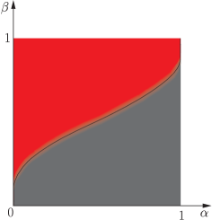
Figure 16: Typical phase transition behavior of a sparsity promoting algorithm. Black corresponds to 100% success of recovering the sparsest solution and red to 0%. For high dimensional spaces, the transition is very sharp, as it is the case in the figure. For lower dimensionality spaces, the transition from black to red is smoother and involves a region of varying color intensity.

The reader may already be aware of the fact that, so far, we have avoided to talk about the performance of individual algorithms. We have just discussed some “typical” behavior that algorithms tend to exhibit in practice. What the reader might have expected is to discuss comparative performance tests and draw related conclusions. We have not done it since we feel that it is early in time to have “definite” performance conclusions, and this field is still in an early stage. Most authors compare their newly suggested algorithm with a few other algorithms, usually within a certain algorithmic family and, more important, under some specific scenarios, where the advantages of the newly suggested algorithm are documented. However, the performance of an algorithm can change significantly by changing the experimental scenario, under which the tests are carried out. The most comprehensive comparative performance study, so far, has been carried out in [Male 10]. However, even in this one, the scenario of exact measurements has been considered and there are no experiments concerning the robustness of individual algorithms to the presence of noise. It is important to say that this study involved a huge effort of computation. We will comment on some of the findings from this study, which will also reveal to the reader that different experimental scenarios can significantly affect the performance of an algorithm.

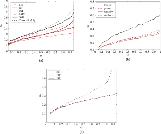
Figure 17: (a) The obtained phase transition curves for different algorithms under the same experimental scenario, together with the theoretical one. (b) Phase transition curve for the IST algorithm under different experimental scenarios for generating the target sparse vector. (c) The phase transition for the IST algorithms under different experimental scenarios for generating the sensing matrix $X$.

Fig. 17a shows the obtained phase transition curves for a) the iterative hard thresholding (IHT), b) the iterative soft thresholding scheme of (48) (IST), c) the Two-Stage-Thresholding scheme (TST), as discussed earlier on, d) the LARS and e) the OMP algorithms, together with the theoretically obtained one using $\ell_{1}$ minimization. All algorithms were tuned with the optimal values, with respect to the required user-defined parameters, after extensive experimentation. The results in the Figure correspond to the uniform spherical scenario, for the generation of the sensing matrices. Sparse vectors were generated according to the $\pm 1$ scenario, for the nonzero coefficients. The interesting observation is that, although the curves deviate from each other as we move to larger values of $\beta$, for smaller values, the differences in their performance become less and less. This is also true for computationally simple schemes, such as the IHT one. The performance of LARS is close to the optimal one. However, this comes at the cost of computational increase. The required computational time for achieving the same accuracy, as reported in [Male 10], favor the TST algorithm. In some cases, LARS required excessively longer time to reach the same accuracy, in particular when the sensing matrix was the partial Fourier one and fast schemes to perform matrix vector products can be exploited. For such matrices, the thresholding schemes (IHT, IST, TST) exhibited a performance that scales very well to large size problems.

Fig. 17b indicates the phase transition curve for one of the algorithms (IST) as we change the scenarios for generating the sparse (target) vectors, using different distributions; a) $\pm 1$, with equiprobable selection of signs (Constant Amplitude Random Selection (CARS)), b) double exponential (power), c) Cauchy and d) uniform in $[-1,1]$. This is indicative and typical for other algorithms as well, with some of them being more sensitive than others. Finally, Fig. 17c shows the transition curves for the IST algorithm by changing the sensing matrix generation scenario. Three curves are shown corresponding to a) uniform spherical ensemble (USE), b) random sign ensemble (RSE), where the elements are $\pm 1$ with signs uniformly distributed and c) the uniform random projection (URP) ensemble. Once more, one can observe the possible variations that are expected due to the use of different matrix ensembles. Moreover, changing ensembles affects each algorithm in a different way.

Concluding this section it must be emphasized that the field of algorithmic development is still an ongoing research field and it is early to come with definite and concrete comparative performance conclusions. Moreover, besides the algorithmic front, existing theories often fall short to predict what is observed in practice, with respect to their phase transition performance. For a related discussion, see, e.g., [Dono 10b].

Example 5.

We are given a set of $N=20$ measurements stacked in the $\bm{y}\in\mathcal{R}^{N}$ vector. These were taken by applying a sensing matrix $X$ on an “unknown” vector in $\mathcal{R}^{50}$, which is known to be sparse with $k=5$ nonzero components; the location of these nonzero components in the unknown vector are not known. The sensing matrix was a random matrix with elements drawn from a normal distribution $\mathcal{N}(0,1)$ and then the columns were normalized to unit norm. There are two scenarios for the measurements. In the first one, we are given the exact measurements while in the second one white Gaussian noise of variance $\sigma^{2}=0.025$ was added.

In order to recover the unknown sparse vector, the CoSaMP algorithm was used for both scenarios.

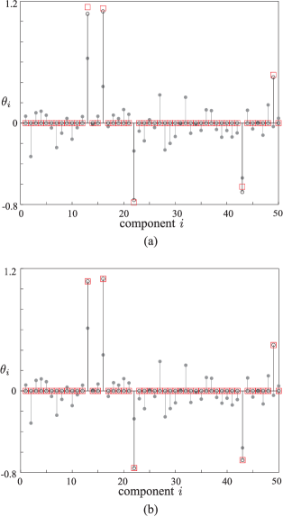
Figure 18: (a) Noiseless case. The values of the true vector, which generated the data for the Example 5, are shown with stems topped with open circles. The recovered points, using the CoSaMP, are shown with squares. An exact recovery of the signal has been obtained. The stems topped with gray circles correspond to the minimum Euclidean norm LS solution. (b) This figure corresponds to the noisy counterpart of that in (a) In the presence of noise, exact recovery is not possible and the more the power of the noise is the less accurate the results are.

The results are shown in Figs. 18a and 18b for the noiseless and noisy scenarios, respectively. The values of the true unknown vector $\bm{\theta}$ are represented with black stems topped with open circles. Note that all but five of them are zero. In Fig. 18a exact recovery of the unknown values is succeeded; the estimated values of $\theta_{i},i=1,2\ldots,50$, are indicated with squares in red color. In the noisy case of Fig. 18b, the resulted estimates, which are denoted with squares, deviate from the correct values. Note that estimated values very close to zero ($|\theta|\leq 0.01$) have been omitted from the figure in order to facilitate visualizing. In both figures, the stemmed gray filled circles correspond to the minimum $\ell_{2}$ norm LS solution. The advantages of adopting a sparsity-promoting approach to recover the solution are obvious. The CoSaMP algorithm was provided with the exact number of sparsity. The reader is advised to play with this example by experimenting with different values of the parameters and see how results are affected.

12 Variations on the Sparsity-Aware Theme

In our tour, so far, we have touched a number of aspects of the sparsity-aware learning that come from the main stream of the theoretical developments. However, more and more variants appear, which are developed with the goal to address problems of a more special structure and/or to propose alternatives, which can be beneficial in boosting the performance in practice, by serving the needs of specific applications. These variants focus either on the regularization term in (13) or on the misfit-measuring term or on both. Once more, research activity in this direction is dense and our purpose is to simply highlight possible alternatives and make the reader alert of the various possibilities that spring from the basic theory.

In a number of tasks, it is a-priori known that the nonzero coefficients in the target signal/vector occur in groups and they are not randomly spread in all possible positions. Such a typical example is the echo path in internet telephony, where the nonzero coefficients of the impulse response tend to cluster together, see Fig. 6. Other examples of “structured” sparsity can be traced in DNA microarrays, MIMO channel equalization, source localization in sensor networks, magnetoencephalography or in neuroscience problems, e.g., [Bara 10b, Parv 08, Garr 08, Bara 10a]. As it is always the case in Machine Learning, being able to incorporate a-priori information in the optimization can only be of benefit for improving performance, since the estimation task is externally assisted in its effort to search for the target solution.

The group LASSO, [Baki 99, Yuan 07, Oboz 06, Frie 10] addresses the task where it is a-priori known that the nonzero components occur in groups. The unknown vector $\bm{\theta}$ is divided into, say, $L$ groups, i.e.,

$$\bm{\theta}^{T}=[\bm{\theta}^{T}_{1},\ldots,\bm{\theta}^{T}_{L}]^{T},$$

each of them of a predetermined size, $s_{i},~{}i=1,2,\ldots,L$, with $\sum_{i=1}^{L}s_{i}=l$. The regression model can then be written as

$$\bm{y}=X\bm{\theta}+\bm{\eta}=\sum_{i=1}^{L}X_{i}\bm{\theta}_{i}+\bm{\eta},$$

where each $X_{i}$ is a submatrix of $X$ comprising the corresponding $s_{i}$ columns. The solution of the group LASSO is given by the following LS regularized task

$$\hat{\bm{\theta}}=\operatorname{arg\,min}_{\bm{\theta}\in{\cal R}^{l}}\left(\left\|{\bm{y}-\sum_{i=1}^{L}X_{i}\bm{\theta}_{i}}\right\|^{2}_{2}+\lambda\sum_{i=1}^{L}\sqrt{s_{i}}\left\|{\bm{\theta}_{i}}\right\|_{2}\right),$$ (59)

where $\left\|{\bm{\theta}_{i}}\right\|_{2}$ is the Euclidean norm (not the squared one) of $\bm{\theta}_{i}$, i.e.,

$$\left\|{\bm{\theta}_{i}}\right\|_{2}=\sqrt{\sum_{j=1}^{s_{i}}|\theta_{i,j}|^{2}}.$$

In other words, the individual components of $\bm{\theta}$ that contribute to the formation of the $\ell_{1}$ norm, in the standard LASSO formulation are now replaced by the square root of the energy of each individual block. In this setting, it is not the individual components but blocks of them which are forced to zero, when their contribution to the LS misfit measuring term is not significant. Sometimes, this type of regularization is coined as the $\ell_{1}/\ell_{2}$ regularization. It is straightforward to see that if $L=l$, then the group LASSO becomes the standard LASSO method. An alternative formulation of the group sparse model using greedy algorithms is considered in [Elda 10]. Theoretical results that extend the RIP to the so-called block RIP have been developed and reported, see, e.g., [Blum 09b, Lu 08a].

In [Cevh 09, Bara 10b], the so-called model based Compressed Sensing is addressed. The $(k,C)$ model allows the significant coefficients of a $k$-sparse signal to appear in at most $C$ clusters, whose size is unknown. This is a major difference with the group LASSO, that was reported before. In Section 10, it was commented that searching for a $k$-sparse solution takes place in a union of subspaces, each one of dimensionality $k$. Imposing a certain structure on the target solution restricts the searching in a subset of these subspaces and leaves a number of these out of the game. This obviously facilitates the optimization task. In [Cevh 09], a dynamic programming technique is adopted to obtain the solution. In [Cevh 10], structured sparsity is considered in terms of graphical models. An even more advanced block sparsity model is the C-HiLasso, which allows each block to have a sparse structure itself, [Spre 11].

Figure 19: (a) The isovalue curves for the $\ell_{1}$ and the weighted $\ell_{1}$ norms for the same value. The weighted $\ell_{1}$ is sharply pinched around one of the axis, depending on the weights. (b) Adopting to minimize the weighted $\ell_{1}$ norm, for the setup of Figure 10 the correct sparse solution is obtained.

In [Cand 08b], it is suggested to replace the $\ell_{1}$ norm by a weighted version of it. To justify such a choice, let us recall Example 2 and the case where the “unknown” system was sensed using $\bm{x}=[2,1]^{T}$. We have seen that by “blowing” up the $\ell_{1}$ ball, the wrong sparse solution was obtained. Let us now replace the $\ell_{1}$ norm in (28) with its weighted version

$$\left\|{\bm{\theta}}\right\|_{1,w}\coloneqq w_{1}|\theta_{1}|+w_{2}|\theta_{2}|,\quad w_{1},w_{2}>0,$$

and set $w_{1}=4$ and $w_{1}=1$. Fig. 19a shows the isovalue curve $\left\|{\bm{\theta}}\right\|_{1,w}=1$, together with that resulting from the standard $\ell_{1}$ norm. The weighted one is sharply “pinched” around the vertical axis, and the larger the value of $w_{1}$ is, compared to that of $w_{2}$, the sharper the corresponding ball will be. Fig. 19b shows what happens when “blowing” the weighted $\ell_{1}$ ball. It will first touch the point $(0,1)$, which is the true solution. Basically, what we have done is to “squeeze” the $\ell_{1}$ ball to be aligned more to the axis that contains the (sparse) solution. For the case of our example, any weight $w_{1}>2$ would do the job.

Considering now the general case of a weighted norm

$$\left\|{\bm{\theta}}\right\|_{1,w}\coloneqq\sum_{j=1}^{l}w_{j}|\theta_{j}|,\quad w_{j}>0.$$

The ideal choice of the weights would be

$$w_{j}=\begin{cases}\frac{1}{|\theta_{0,j}|},&\theta_{0,j}\neq 0,\\ \infty,&\theta_{0,j}=0,\end{cases}$$

where $\bm{\theta}_{0}$ is the target true vector, and where we have silently assumed that $0\cdot\infty=0$. In other words, the smaller a coefficient is the larger the respective weight becomes. This is justified, since large weighting will force respective coefficients towards zero during the minimization process. Of course, in practice the values of the true vector are not known, so it is suggested to use their estimates during each iteration of the minimization procedure. The resulting scheme is of the following form.

Algorithm 3.

1. Initialize weights to unity, $w^{(0)}_{j}=1$, $j=1,2,\ldots,l$.

2. Minimize the weighted $\ell_{1}$ norm,

   $$\bm{\theta}^{(i)} = \operatorname{arg\,min}_{\bm{\theta}\in\mathcal{R}^{l}}\left\|{\bm{\theta}}\right\|_{1,w}$$

   $$\text{s.t.}\ \bm{y}=X\bm{\theta}.$$

3. Update the weights

   $$w_{j}^{(i+1)}=\frac{1}{\left|\theta_{j}^{(i)}\right|+\epsilon},\quad j=1,2,\ldots,l.$$

4. Terminate when a stopping criterion is met, otherwise return to step 2.

The constant $\epsilon$ is a small user-defined parameter to guarantee stability when the estimates of the coefficients take very small values. Note that if the weights have constant preselected values, the task retains its convex nature; this is no longer true when the weights are changing. It is interesting to point out that this intuitively motivated weighting scheme can result if the $\ell_{1}$ norm is replaced by $\sum_{j=1}^{l}\ln\left(|\theta_{j}|+\epsilon\right)$ as the regularizing term of (13). Fig. 20 shows the respective graph, in the one-dimensional space together with that of the $\ell_{1}$ norm. The graph of the logarithmic function reminds us of the $\ell_{p}$, $p<0<1$, “norms” and the comments made in Section 3. This is no more a convex function and the iterative scheme, given before, is the result of a majorization-minimization procedure in order to solve the resulting non-convex task, [Cand 08b].

Figure 20: One-dimensional graphs of the $\ell_{1}$ norm and the logarithmic regularizer $\ln\bigl{(}\frac{|\theta|}{\epsilon}+1\bigr{)}=\ln\bigl{(}|\theta|+\epsilon\bigr{)}-\ln\epsilon$, with $\epsilon=0.1$. The term $\ln\epsilon$ was subtracted for illustration purposes only and does not affect the optimization. Notice the nonconvex nature of the logarithmic regularizer.

The concept of the iterative weighting, as used before, has also been applied in the context of the iterative reweighted least squares algorithm. Observe that the $\ell_{1}$ norm can be written as

$$\left\|{\bm{\theta}}\right\|_{1}=\sum_{j=1}^{l}|\theta_{j}|=\bm{\theta}^{T}\mathcal{W}_{\theta}\bm{\theta},$$

where

$$\mathcal{W}_{\theta}=\begin{bmatrix}\frac{1}{|\theta_{1}|}&0&\cdots&0\\ 0&\frac{1}{|\theta_{2}|}&\cdots&0\\ \vdots&\vdots&\ddots&\vdots\\ 0&0&\cdots&\frac{1}{|\theta_{l}|}\end{bmatrix},$$

and where in the case of $\theta_{i}=0$, for some $i\in\{1,2,\ldots,l\}$, the respective coefficient of $\mathcal{W}_{\theta}$ is defined to be $1$. If $\mathcal{W}_{\theta}$ were a constant weighting matrix, i.e., $\mathcal{W}_{\theta}\coloneqq\mathcal{W}_{\tilde{\theta}}$, for some fixed $\tilde{\bm{\theta}}$, then obtaining the minimum

$$\hat{\bm{\theta}}=\operatorname{arg\,min}_{\bm{\theta}\in\mathcal{R}^{l}}\left\|{\bm{y}-X\bm{\theta}}\right\|^{2}_{2}+\lambda\bm{\theta}^{T}\mathcal{W}_{\tilde{\theta}}\bm{\theta},$$

is straightforward and similar to the ridge regression. In the iterative reweighted scheme, $\mathcal{W}_{\theta}$ is replaced by $\mathcal{W}_{{\theta}^{(i)}}$, formed by using the respected estimates of the coefficients which have been obtained from the previous iteration, i.e., $\tilde{\bm{\theta}}\coloneqq\bm{\theta}^{(i)}$, as we did before. In the sequel, each iteration solves a weighted ridge regression task. Variants of this basic iteratively weighting scheme have also been proposed, see, e.g., [Daub 10] and the references therein.

In [Cand 07], the LASSO task is modified by replacing the square error term with one involving correlations and the minimization task becomes

$$\hat{\bm{\theta}}:\min_{\bm{\theta}\in\mathcal{R}^{l}} \left\|{\bm{\theta}}\right\|_{1}$$

s.t. $$\left\|{X^{T}(\bm{y}-X\bm{\theta})}\right\|_{\infty}\leq\epsilon,$$

where $\epsilon$ is related to $l$ and the noise variance. This task is known as the Dantzig selector. That is, instead of constraining the energy of the error, the constraint, now, imposes an upper limit to the correlation of the error vector with any of the columns of $X$. In [Bick 09, Asif 10b], it is shown that under certain conditions the LASSO estimator and the Dantzig selector become identical.

Total Variation (TV) [Rudi 92] is a closely related to $\ell_{1}$ sparsity promotion notion and it has been widely used in image processing. Most of the grayscale image arrays, $I\in\mathcal{R}^{l\times l}$, consist of slowly varying pixel intensities except at the edges. As a consequence, the discrete gradient of an image array will be approximately sparse (compressible). The discrete directional derivatives of an image array are defined pixel-wise as

$$\nabla_{x}(I)(i,j) \coloneqq I(i+1,j)-I(i,j),\quad\forall i\in\{1,2,\ldots,l-1\},$$ (60)

$$\nabla_{y}(I)(i,j) \coloneqq I(i,j+1)-I(i,j),\quad\forall j\in\{1,2,\ldots,l-1\},$$ (61)

and

$$\nabla_{x}(I)(l,j)\coloneqq\nabla_{y}(I)(i,l)\coloneqq 0,\quad\forall i,j\in\{1,2,\ldots,l-1\}.$$ (62)

The discrete gradient transform

$$\nabla:\mathcal{R}^{l\times l}\rightarrow\mathcal{R}^{l\times 2l},$$

is defined in terms of a matrix form as

$$\nabla(I)(i,j)\coloneqq[\nabla_{x}(i,j),\nabla_{y}(i,j)],\quad\forall i,j\in\{1,2,\ldots l\}.$$ (63)

The total variation of the image array is defined as the $\ell_{1}$ norm of the magnitudes of the elements of the discrete gradient transform, i.e.,

$$\left\|{I}\right\|_{\text{TV}}\coloneqq\sum_{i=1}^{l}\sum_{j=1}^{l}\left\|{\nabla(I)(i,j)}\right\|_{2}=\sum_{i=1}^{l}\sum_{j=1}^{l}\sqrt{\nabla_{x}(I)^{2}(i,j)+\nabla_{y}(I)^{2}(i,j)}.$$ (64)

Note that this is a mixture of $\ell_{2}$ and $\ell_{1}$ norms. The sparsity promoting optimization around the total variation is defined as

$$I_{*} \in \mbox{arg}\min_{I}\left\|{I}\right\|_{TV}$$ (65)

$$\text{s.t.}\ \left\|{\bm{y}-\mathcal{F}(I)}\right\|_{2}\leq\epsilon,$$

where $\bm{y}\in\mathcal{R}^{N}$ is the measurements vector and $\mathcal{F}(I)$ denotes the result in vectorized form of the application of a linear operator on $I$. For example, this could be the result of the action of a partial two-dimensional DFT on the image. Subsampling of the DFT matrix as a means to form sensing matrices has already been discussed in Section 8.2. The task in (65) retains its convex nature and it basically expresses our desire to reconstruct an image which is as smooth as possible given the available measurements. The NESTA algorithm can be used for solving the total variation minimization task; besides it, other efficient algorithms for this task can be found in, e.g., [Gold 09, Yang 10].

It has been shown in [Cand 06a], for the exact measurements case $(\epsilon=0)$, and in [Need 12], for the erroneous measurements case, that conditions and bounds which guarantee recovery of an image array from the task in (65) can be derived and are very similar with those that we have discussed for the case of the $\ell_{1}$ norm.

Example 6 (Magnetic Resonance Imaging (MRI)).

In contrast to ordinary imaging systems, which directly acquire pixel samples, MRI scanners sense the image in an encoded form. Specifically, MRI scanners sample components in the spatial frequency domain, known as “$k$-space” in the MRI nomenclature. If all the components in this transform domain were available, one could apply the inverse 2D-DFT to recover the exact MR image in the pixel domain. Sampling in the $k$-space is realized along particular trajectories in a number of successive acquisitions. This process is time consuming, merely due to physical constraints. As a result, techniques for efficient image recovery from a limited number of measurements is of high importance, since they can reduce the required acquisition time for performing the measurements. Long acquisition times are not only inconvenient but even impossible, since the patients have to stay still for long time intervals. Thus, MRI was among the very first applications where compressed sensing found its way to offer its elegant solutions.

Fig. 21a shows the “famous” Shepp-Logan phantom, and the goal is to recover it via a limited number of (measurements) samples in its frequency domain. The MRI measurements are taken across 17 radial lines in the spatial frequency domain, as shown in Fig. 21(b). A “naive” approach to recover the image from this limited number of measuring samples would be to adopt a zero-filling rationale for the missing components. The recovered image according to this technique is shown in Fig. 21(c). Fig. 21(d) shows the recovered image using the approach of minimizing the total variation, as explained before. Observe that the results for this case are astonishingly good. The original image is almost perfectly recovered. The constrained minimization was performed via the NESTA algorithm. Note that if the minimization of the $\ell_{1}$ norm of the image array were used in place of the total variation, the results would not be as good; the phantom image is sparse in the discrete gradient domain, since it contains large sections which share constant intensities.

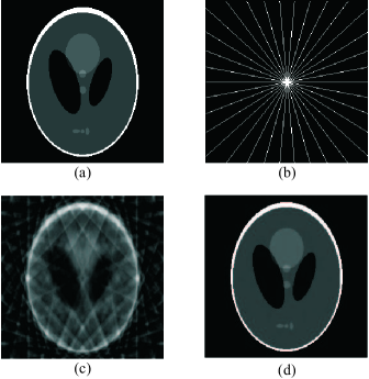
Figure 21: a) The original Shepp-Logan image phantom. b) The white lines indicate the directions across which the sampling in the spatial Fourier transform were obtained. c) The recovered image after applying the inverse DFT having first filled with zeros the missing values in the DFT transform. d) The recovered image using the total variation minimization approach.

13 Online Time-Adaptive Sparsity-Promoting Algorithms

In this section, online (time-recursive) schemes for sparsity-aware learning are presented. There is a number of reasons that one has to resort to such schemes in various signal processing tasks, for example, when the data arrive sequentially. Under such a scenario, using batch processing techniques to obtain an estimate of an unknown target parameter vector would be highly inefficient, since the number of training points keeps increasing. Such an approach is prohibited for real time applications. Moreover, time-recursive schemes can easily incorporate the notion of adaptivity, when the learning environment is not stationary but it undergoes changes as time evolves. Besides signal processing applications, there is an increasing number of machine learning applications where online processing is of paramount importance, such as bioinformatics, hyperspectral imaging, and data mining. In such applications, the number of training points easily amounts to a few thousand up to hundred of thousand points. Concerning the dimensionality of the ambient (feature) space, one can claim numbers that lie in similar ranges. For example, in [Lang 09], the task is to search for sparse solutions in feature spaces with dimensionality as high as $10^{9}$ having access to data sets as large as $10^{7}$ points. Using batch techniques, in a single computer, is out of question with today’s technology.

Let us assume that there is an unknown parameter vector that generates data according the standard regression model

$$y_{n}=\bm{x}_{n}^{T}\bm{\theta}+\eta_{n},\quad\forall n,$$

and the training samples are received sequentially $(y_{n},\bm{x}_{n})$, $n=1,2,\ldots$. In the case of a stationary environment, we would expect our algorithm to converge, asymptotically as $n\rightarrow\infty$, to or “near to” the true parameter vector that gives birth to the measurements, $y_{n}$, when it is sensed by $\bm{x}_{n}$. For time varying environments, the algorithms should be able to track the underlying changes as time goes by. Before we proceed, a comment is important. Since the time index, $n$, is left to grow, all we have said in the previous sections with respect to underdetermined systems of equations, looses its meaning. Sooner or later we are going to have more measurements than the dimensionality of the space. Our major concern here becomes the issue of asymptotic convergence, for the case of stationary environments. The obvious question, that is now raised, is why not using a standard algorithm, e.g., LMS, RLS or APSM [Saye 03, Hayk 96, Theo 11], since we know that these algorithms converge to, or near enough in some sense, to the solution; that is, the algorithm will identify the zeros asymptotically. The answer is that if such algorithms are modified to be aware for the underlying sparsity, convergence is significantly speeded up; in real life applications, one has not the “luxury” to wait long time for the solution. In practice, a good algorithm should be able to provide a good enough solution, and in the case of sparse solutions to obtain the support, after a reasonably small number of iteration steps. In this section, the powerful theory around the $\ell_{1}$ norm regularization will be used to obtain sparsity-aware time adaptive schemes.

13.1 LASSO: Asymptotic Performance

The notions of bias, variance and consistency, are major indices for assessing the performance of an estimator. In a number of cases, such performance measures are derived asymptotically. For example, it is well known that the maximum likelihood estimator is asymptotically unbiased and consistent [Theo 09]. Also the LS estimator is asymptotically consistent. Moreover, under the assumption that the noise samples are i.i.d., the LS estimate, $\hat{\bm{\theta}}_{N}$, that is obtained using $N$ measurement (training) samples, is itself a random vector, that satisfies the $\sqrt{N}$-estimation consistency, e.g., [Kay 93], i.e.,

$$\sqrt{N}\left(\hat{\bm{\theta}}_{N}-\bm{\theta}_{0}\right)\xrightarrow{d}\mathcal{N}\left(\bm{0},\sigma^{2}\Sigma^{-1}\right),$$

where $\bm{\theta}_{0}$ is the true vector that generates the measurements, $\sigma^{2}$ denotes the variance of the noise source and $\Sigma$ is the covariance matrix $\operatorname{\mathsf{E}}[\bm{x}\bm{x}^{T}]$ of the input sequence, which has been assumed to be zero mean and the limit denotes convergence in distribution.

The LASSO in (13) is the task of minimizing the $\ell_{1}$ norm regularized version of the LS cost. However, nothing has been said, so far, about the statistical properties of this estimator. The only performance measure that we referred to was the error norm bound given in (43). However, this bound, although important in the context it was proposed for, does not provide much statistical information. Since the introduction of the LASSO estimator, a number of papers have addressed problems related to its statistical performance, see, e.g., [Dono 95, Knig 00, Fan 01, Zou 06].

When dealing with sparsity-promoting estimators, such as the LASSO, two crucial issues emerge: a) whether the estimator, even asymptotically, can obtain the support, if the true vector parameter is a sparse one and b) quantify the performance of the estimator with respect to the estimates of the nonzero coefficients, i.e., those whose index belongs to the support. Especially for LASSO, the latter issue becomes to study whether LASSO behaves as well as the unregularized LS with respect to these nonzero components. This task was addressed, for a first time and in a more general setting, in [Fan 01]. Let the support of the true, yet unknown, $k$-sparse parameter vector $\bm{\theta}_{0}$ be denoted as $S$. Let also $\Sigma_{|S}$ be the $k\times k$ covariance matrix $\operatorname{\mathsf{E}}[\bm{x}_{|S}\bm{x}_{|S}^{T}]$, where $\bm{x}_{|S}\in\mathcal{R}^{k}$ is the vector that contains only the $k$ components of $\bm{x}$, with indices in the support $S$. Then, we say that an estimator satisfies asymptotically the oracle properties if:

• $\lim_{N\rightarrow\infty}\operatorname{Prob}\left\{S_{\hat{\bm{\theta}}_{N}}=S\right\}=1$. This is known as support consistency.

• $\sqrt{N}\left(\hat{\bm{\theta}}_{N|S}-\bm{\theta}_{0|S}\right)\xrightarrow{d}\mathcal{N}\left(\bm{0},\sigma^{2}\Sigma^{-1}_{|S}\right)$. This is the $\sqrt{N}$-estimation consistency.

We denote as $\bm{\theta}_{0|S}$ and $\bm{\theta}_{N|S}$ the $k$-dimensional vectors which result from $\bm{\theta}_{0},~{}\hat{\bm{\theta}}_{N}$, respectively, if we keep the components whose indices lie in the support $S$. In other words, according to the oracle properties, a good sparsity-promoting estimator should be able a) to predict, asymptotically, the true support and b) its performance with respect to the nonzero components should be as good as that of a genie-aided LS estimator, which is informed, in advance, of the positions of the nonzero coefficients.

Unfortunately, the LASSO estimator cannot satisfy simultaneously both conditions. It has been shown, [Knig 00, Fan 01, Zou 06] that:

• For support consistency, the regularization parameter $\lambda\coloneqq\lambda_{N}$ should be time varying such as

  $$\lim_{N\rightarrow\infty}\frac{\lambda_{N}}{\sqrt{N}}=\infty,\quad\lim_{N\rightarrow\infty}\frac{\lambda_{N}}{N}=0.$$

  That is, $\lambda_{N}$ must grow faster than $\sqrt{N}$, but slower than $N$.

• For $\sqrt{N}$-consistency, $\lambda_{N}$ must grow as

  $$\lim_{N\rightarrow\infty}\frac{\lambda_{N}}{\sqrt{N}}=0,$$

  i.e., it grows slower than $\sqrt{N}$.

The previous two conditions are conflicting and the LASSO estimator cannot comply with the two oracle conditions simultaneously. The proofs of the previous two points are somewhat technical and are not given here. The interested reader can obtain them from the previously given references. However, before we proceed, it is instructive to see why the regularization parameter has to grow slower than $N$, in any case. Without being too rigorous mathematically, recall that the LASSO solution comes from equation (13). This can be written as

$$\bm{0}\in-\frac{2}{N}\sum_{n=1}^{N}\bm{x}_{n}y_{n}+\frac{2}{N}\left(\sum_{n=1}^{N}\bm{x}_{n}\bm{x}_{n}^{T}\right)\bm{\theta}+\frac{\lambda_{N}}{N}\partial\left\|{\bm{\theta}}\right\|_{1},$$ (66)

where we have divided by $N$ both sides. Taking the limit as $N\rightarrow\infty$, if $\lambda_{N}/N\rightarrow 0$, then we are left with the first two terms; this is exactly what we would have if the unregularized LS had been chosen as the cost function. In this case, the solution asymptotically converges (under some general assumptions, which are assumed to hold true, here) to the true parameter vector; that is, we have strong consistency, e.g., [Kay 93].

13.2 The Adaptive Norm-Weighted LASSO

There are two ways to get out of the previously stated conflict. One is to replace the $\ell_{1}$ norm with a nonconvex function and this can lead to an estimator that satisfies the oracle properties simultaneously [Fan 01]. The other is to modify the $\ell_{1}$ norm by replacing it with a weighted version. Recall that the weighted $\ell_{1}$ norm was discussed in Section 12, as a means to assist the optimization procedure to unveil the sparse solution. Here the notion of weighted $\ell_{1}$ norm comes as a necessity imposed by our willingness to satisfy the oracle properties. This gives rise to the adaptive norm-weighted LASSO cost estimator defined as

$$\hat{\bm{\theta}}=\operatorname{arg\,min}_{\bm{\theta}\in\mathcal{R}^{l}}\left\{\sum_{j=1}^{n}\beta^{n-j}\left(y_{j}-\bm{x}_{j}^{T}\bm{\theta}\right)^{2}+\lambda_{n}\sum_{i=1}^{l}w_{i}(n)|\theta_{i}|\right\},$$ (67)

where $\beta\leq 1$ is used as the forgetting factor to allow for tracking slow variations. The time varying weighting sequences is denoted as $w_{i}(n)$. There are different options. In [Zou 06] and under a stationary environment with $\beta=1$, it is shown that if

$$w_{i}(n)=\frac{1}{|\theta_{i}^{\text{est}}|^{\gamma}},$$

where $\theta_{i}^{\text{est}}$ is the estimate of the $i$th component obtained by any $\sqrt{n}$-consistent estimator, such as the unregularized LS, then for specific choices of $\lambda_{n}$ and $\gamma$ the estimator satisfies the oracle properties simultaneously. The main reasoning behind the weighted norms is that as time goes by, and the $\sqrt{n}$-consistent estimator provides better and better estimates, then the weights corresponding to indices outside the true support (zero values) are inflated and those corresponding to the true support converge to a finite value. This helps the algorithm, simultaneously, to locate the support and obtain unbiased (asymptotically) estimates of the large coefficients.

Another choice for the weighing sequence is related to the so called Smoothly Clipped Absolute Deviation (SCAD) [Fan 01, Zou 08]. This is defined as

$$w_{i}(n)=\chi_{(0,\mu_{n})}(|\theta^{\text{est}}_{i}|)+\frac{\left(\alpha\mu_{n}-|\theta_{i}^{\text{est}}|\right)_{+}}{(\alpha-1)\mu_{n}}\chi_{(\mu_{n},\infty)}(|\theta^{\text{est}}_{i}|),$$

where $\chi(\cdot)$ stands for the characteristic function, $\mu_{n}=\lambda_{n}/n$, and $\alpha>2$. Basically, this corresponds to a quadratic spline function. It turns out, [Zou 08], that if $\lambda_{n}$ is chosen to grow faster that $\sqrt{n}$ and slower that $n$, the adaptive LASSO, with $\beta=1$ satisfies both oracle conditions, simultaneously.

A time adaptive scheme for solving the time adaptive norm-weighted (TNWL) LASSO was presented in [Ange 10]. The cost function of the adaptive LASSO in (67) can be written as

$$J(\bm{\theta})=\bm{\theta}^{T}R_{n}\bm{\theta}-\bm{r}_{n}^{T}\bm{\theta}+\lambda_{n}\left\|{\bm{\theta}}\right\|_{1,w(n)},$$

where

$$R_{n}\coloneqq\sum_{j=1}^{n}\beta^{n-j}\bm{x}_{j}\bm{x}_{j}^{T},\quad\bm{r}_{n}\coloneqq\sum_{j=1}^{n}\beta^{n-j}y_{j}\bm{x}_{j},$$

and $\left\|{\bm{\theta}}\right\|_{1,w(n)}$ is the weighted $\ell_{1}$ norm. It is straightforward to see, that

$$R_{n}=\beta R_{n-1}+\bm{x}_{n}\bm{x}_{n}^{T},\quad\bm{r}_{n}=\beta\bm{r}_{n-1}+y_{n}\bm{x}_{n}.$$

The complexity for both of the previous updates, for matrices of a general structure, amounts to $\mathcal{O}(l^{2})$ multiply/add operations. One alternative is to update $R_{n}$ and $\bm{r}_{n}$ and then solve a convex optimization task for each time instant, $n$, using any standard algorithm. However, this is not appropriate for real time applications, due to its excessive computational cost. In [Ange 10], a time recursive version of a coordinate descent algorithm has been developed. As we have seen in Section 11.2, coordinate descent algorithms update one component at each recursive step. In [Ange 10], recursive steps are associated with time updates, as it is always the case with the time-recursive algorithms. As each new training pair $(y_{n},\bm{x}_{n})$ is received, a single component of the unknown vector is updated. Hence, at each time instant, a scalar optimization task has to be solved and its solution is given in closed form, which results in a simple soft thresholding operation (OCCD-TWL). If the weighted norm is to be used in place of the $\ell_{1}$, a RLS is run in parallel to provide the necessary weights. One of the drawbacks of the coordinate techniques is that each coefficient is updated every $l$ time instants, which, for large values of $l$, can slow down convergence. Variants of the basic scheme that cope with this drawback are also addressed in [Ange 10], referred  to as online cyclic coordinate descent (OCCD-TNWL). The complexity of the scheme is of the order of $\mathcal{O}(l^{2})$. Computational savings are possible, if the input sequence is a time series and fast schemes for the updates of $R_{n}$ and the RLS can then be exploited. However, if an RLS-type algorithm is used in parallel, the convergence of the overall scheme may be slowed down, since the RLS-type algorithm has to converge first, in order to provide reliable estimates for the weights, as pointed out before.

13.3 Adaptive CoSaMP Algorithm (AdCoSaMP)

In [Mile 10], an adaptive version of the CoSaMP algorithm, which was presented in Section 11.1.3, was proposed. Iteration steps, $i$, now coincide with time updates, $n$, and the LS solver in Step 3c of the general CSMP scheme is replaced by an LMS one.

Let us focus first on the quantity $X^{T}\bm{e}^{(i-1)}$ in Step 3a of the CSMP scheme, which is used to compute the support at iteration $i$. In the adaptive setting and at (iteration) time $n$, this quantity is now “rephrased” as

$$X^{T}\bm{e}(n-1)=\sum_{j=1}^{n-1}\bm{x}_{j}e(j).$$

In order to make the algorithm flexible to adapt to variations of the environment, as the time index, $n$, increases, the previous correlation sum is modified to

$$\bm{p}(n):=\sum_{j=1}^{n-1}\beta^{n-1-j}\bm{x}_{j}e(j)=\beta\bm{p}(n-1)+\bm{x}_{n-1}e(n-1).$$

The LS task, constrained on the active columns that correspond to the indices in the support $S$ in Step 3c, is performed in an adaptive rationale by involving the basic LMS recursions, i.e.,

$$\tilde{e}(n) \coloneqq y_{n}-\bm{x}_{n|S}^{T}\tilde{\bm{\theta}}_{|S}(n-1)$$

$$\tilde{\bm{\theta}}_{|S}(n) \coloneqq \tilde{\bm{\theta}}_{|S}(n-1)+\mu\bm{x}_{n|S}\tilde{e}(n),$$

where $\tilde{\bm{\theta}}_{|S}(\cdot)$ and $\bm{x}_{n|S}$ denote the respective subvectors corresponding to the indices in the support $S$. The resulting algorithm is given as follows.

Algorithm 4 (The AdCoSaMP Scheme).

1. Select the value of $t=2k$.

2. Initialize the algorithm: $\bm{\theta}(1)=\bm{0}$, $\tilde{\bm{\theta}}(1)=\bm{0}$, $\bm{p}(1)=\bm{0}$, $e(1)=y_{1}$.

3. Choose $\mu$ and $\beta$.

4. For $n=2,3,\ldots$, execute the following steps.

   1. $\bm{p}(n)=\beta\bm{p}(n-1)+\bm{x}_{n-1}e(n-1)$.

   2. Obtain the current support:

      $$S=\operatorname{supp}\{\bm{\theta}(n-1)\}\cup\left\{\text{indices of the}\ t\ \text{largest}\atop\text{in magnitude components of}\ \bm{p}(n)\right\}.$$

   3. Perform the LMS update:

      $$\tilde{e}(n) = y_{n}-\bm{x}_{n|S}^{T}\tilde{\bm{\theta}}_{|S}(n-1),$$

      $$\tilde{\bm{\theta}}_{|S}(n) = \tilde{\bm{\theta}}_{|S}(n-1)+\mu\bm{x}_{n|S}\tilde{e}(n).$$

   4. Obtain the set $S_{k}$ of the indices of the $k$ largest components of $\tilde{\bm{\theta}}_{|S}(n)$.

   5. Obtain $\bm{\theta}(n)$ such that:

      $$\bm{\theta}_{|S_{k}}(n)=\tilde{\bm{\theta}}_{|S_{k}},\quad\text{and}\ \bm{\theta}_{|S^{c}_{k}}(n)=\bm{0},$$

      where $S_{k}^{c}$ is the complement set of $S_{k}$.

   6. Update the error: $e(n)=y_{n}-\bm{x}_{n}^{T}\bm{\theta}(n)$.

In place of the standard LMS, its normalized version can alternatively be adopted. Note that Step 4e is directly related to the hard thresholding operation.

In [Mile 10], it is shown that if the sensing matrix, which is now time dependent and keeps increasing in size, satisfies a condition similar to RIP, for each time instant, called Exponentially Weighted Isometry Property (ERIP), which depends on $\beta$, then the algorithm asymptotically satisfies an error bound, which is similar to the one that has been derived for CoSaMP in [Need 09], plus an extra term that is due to the excess Mean Square Error, which is the price paid by replacing the LS solver by the LMS.

13.4 Sparse Adaptive Parallel Projection onto Convex Sets Method (SpAPSM)

The APSM family of algorithms is one among the most powerful techniques for adaptive learning [Theo 11]. A major advantage of this algorithmic family is that one can readily incorporate convex constraints. The rationale behind APSM is that since our data are known to be generated by a regression model, then the unknown vector could be estimated by finding a point in the intersection of a sequence of hyperslabs, that are defined by the data points, i.e., $S_{n}[\epsilon]\coloneqq\bigl{\{}\bm{\theta}\in\mathcal{R}^{l}:\left|y_{n}-\bm{x}^{T}_{n}\bm{\theta}\right|\leq\epsilon\bigr{\}}$. Such a model is most natural when the noise is bounded, (which, after all, it is the case in any practical application). In case the noise is assumed unbounded, a choice of $\epsilon$ of the order say, $\sigma$, can guarantee, with high probability, that the unknown solution lies inside these hyperslabs.

The APSM family builds upon the elegant philosophy that runs across the classical projections onto convex sets (POCS) theory. Recall that the basic rationale behind POCS is that starting from an arbitrary point in the space and sequentially projecting onto a finite number of convex sets then the sequence of projections converges, in some sense, into the intersection of all these sets, assuming this is not empty. The theory was extended to embrace the online processing setting in [Yama 04, Ogur 02, Slav 06]. In contrast to the classical POCS theory, here the number of the involved convex sets is infinite. It turns out that, under certain general conditions, a sequence of projections over all these sets also converges to a point in their intersection.

To fit the theory into our needs, the place of the aforementioned convex sets is taken by the hyperslabs, which are formed by the received training data, as mentioned before. Thus, the resulting algorithms involves (metric) projections onto these hyperslabs (see Appendix). However, when dealing with sparse vectors, there is an extra projetion associated with the convex set formed by the $\ell_{1}$ ball; that is, $\left\|{\bm{\theta}}\right\|_{1}\leq\rho$ (see, also, the LASSO formulation (14)). Hence, this task fits nicely in the APSM rationale and the basic recursion can be readily written, without much thought or derivation, as follows; for any arbitrarily chosen initial point $\bm{\theta}(0)$, define $\forall n$,

$$\bm{\theta}(n)\coloneqq P_{B_{\ell_{1}}[\delta]}\Biggl{(}\bm{\theta}(n-1)+\mu_{n}\biggl{(}\frac{1}{q}\sum_{i=n-q+1}^{n}P_{S_{i}[\epsilon]}\bigl{(}\bm{\theta}(n-1)\bigr{)}-\bm{\theta}(n-1)\biggr{)}\Biggr{)}$$

where $P_{S_{i}[\epsilon]}$ is the metric projection onto the hyperslab $S_{i}[\epsilon]$ (see Appendix). Note, that in the previous recursion we have used $q$, instead of one, hyperslabs whose metric projections are averaged out at time $n$. It turns out that such an averaging improves convergence significantly. Parameter $\mu_{n}$ is an extrapolation parameter, which takes values in the interval $(0,2\mathcal{M}_{n})$, where

$$\mathcal{M}_{n}\coloneqq\begin{cases}\frac{\sum_{i=n-q+1}^{n}\omega^{(n)}_{i}\left\|{P_{S_{i}[\epsilon]}(\bm{\theta}(n-1))-\bm{\theta}(n-1)}\right\|^{2}}{\left\|{\sum_{i=n-q+1}^{n}\omega^{(n)}_{i}P_{S_{i}[\epsilon]}(\bm{\theta}(n-1))-\bm{\theta}(n-1)}\right\|^{2}},&\\ &\text{if}\ \left\|{\sum_{i=n-q+1}^{n}\omega^{(n)}_{i}P_{S_{i}[\epsilon]}(\bm{\theta}(n-1))-\bm{\theta}(n-1)}\right\|\neq 0,\\ 1,&\text{otherwise},\end{cases}$$ (68)

and $P_{{B_{\ell_{1}}[\rho]}}(\cdot)$ is the projection operator onto the $\ell_{1}$ ball $B_{\ell_{1}}[\rho]\coloneqq\bigl{\{}\bm{\theta}\in\mathcal{R}^{l}:\left\|{\bm{\theta}}\right\|_{1}\leq\rho\bigr{\}}$, since the solution is constrained to live within this ball. Note, that the previous recursion is analogous to the iterative soft thresholding shrinkage algorithm in the batch processing case, (53). There, we saw that the only difference that the sparsity imposes on an iteration, with respect to its unconstrained counterpart, is an extra soft thresholding. This is exactly the case here. The term in the parenthesis is the iteration for the unconstrained task. Moreover, as it has been shown in [Duch 08], projection on the $\ell_{1}$ ball is equivalent to a soft thresholding operation. It can be shown that the previous iteration converges arbitrarily close to a point in the intersection

$$B_{\ell_{1}}[\delta]\cap\bigcap_{n\geq n_{0}}S_{n}[\epsilon],$$

for some finite value of $n_{0}$ [Yama 04, Ogur 02, Slav 06, Theo 11]. In [Kops 11a, Kops 11b] the weighted $\ell_{1}$ ball has been used to improve convergence as well as the tracking speed of the algorithm, when the environment is time varying. The weights were adopted in accordance to what was discussed in Section 12, i.e.,

$$w_{i}(n)\coloneqq\frac{1}{|\theta_{i}(n-1)|+\acute{\epsilon}_{n}},\quad\forall i\in\{1,2,\ldots,l\},$$

where $(\acute{\epsilon}_{n})_{n\geq 0}$ is a sequence (can be also constant) of small numbers to avoid division by zero. The basic time iteration becomes as follows; for any arbitrarily chosen initial point $\bm{\theta}(0)$, define $\forall n$,

$$\bm{\theta}(n)\coloneqq P_{B_{\ell_{1}}[\bm{w}(n),\rho]}\Biggl{(}\bm{\theta}(n-1)+\mu_{n}\biggl{(}\sum_{i=n-q+1}^{n}\omega^{(n)}_{i}P_{S_{i}[\epsilon]}\bigl{(}\bm{\theta}(n-1)\bigr{)}-\bm{\theta}(n-1)\biggr{)}\Biggr{)},$$ (69)

where $\mu_{n}\in(0,2\mathcal{M}_{n})$ and $\mathcal{M}_{n}$ is given in (68). Fig. 22 illustrates the associated geometry of the basic iteration in $\mathcal{R}^{2}$ and for the case of $q=2$. It comprises two parallel projections on the hyperslabs followed by one projection onto the weighted $\ell_{1}$ ball. In [Kops 11a], it is shown that a good bound for the weighted $\ell_{1}$ norm is the sparsity level $k$ of the target vector, which is assumed to be known and it is a user-defined parameter. In [Kops 11a], it is shown that asymptotically, and under some general assumptions, this algorithmic scheme converges arbitrarily close to the intersection of the hyperslabs with the weighted $\ell_{1}$ balls, i.e.,

$$\bigcap_{n\geq n_{0}}\left(P_{B_{\ell_{1}}[\bm{w}(n),\rho]}\cap S_{j}[\epsilon]\right),$$

for some non-negative integer $n_{0}$. It has to be pointed out that, in the case of weighted $\ell_{1}$ norms, the constraint is time varying and the convergence analysis is not covered by the standard analysis used for APSM, and had to be extended to this more general case. The complexity of the algorithm amounts to $\mathcal{O}(ql)$. The larger the $q$ the faster the convergence rate, at the expense of higher complexity. In [Kops 11b], in order to reduce the dependence of the complexity on $q$, the notion of the sub-dimensional projection is introduced, where projections onto the $q$ hyperslabs could be restricted along the directions of the most significant coefficients, of the currently available estimates. The dependence on $q$ now becomes $\mathcal{O}(qk_{n})$ where $k_{n}$ is the sparsity level of the currently available estimate, which, after a few steps of the algorithm, gets much lower than $l$. The total complexity amounts to $\mathcal{O}(l)+\mathcal{O}(qk_{n})$, per iteration step. This allows the use of large values of $q$, which drives the algorithm to a performance close to that of the adaptive weighted LASSO, at only a small extra computational cost.

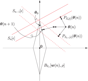
Figure 22: Geometric illustration of the update steps involved in the SpAPSM algorithm, for the case of $q=2$. The update at time $n+1$ is obtained by first convexly combining the projections onto the current and previously formed hyperslabs, $S_{n}[\epsilon],~{}S_{n-1}[\epsilon]$ and then projecting onto the weighted $\ell_{1}$ ball. This brings the update closer to the target solution $\bm{\theta}_{*}$.

13.4.1 Projection onto the Weighted $\ell_{1}$ Ball

Projecting onto an $\ell_{1}$ ball is equivalent to a soft thresholding operation. Projection onto the weighted $\ell_{1}$ norm results to a slight variation of the soft thresholding, with different threshold values per component. In the sequel, we give the iteration steps for the more general case of the weighted $\ell_{1}$ ball. The proof is a bit technical and lengthy and it will not be given here. It was derived, for the first time, via purely geometric arguments, and without the use of the classical Lagrange multipliers, in [Kops 11a]. Lagrange multipliers have been used instead in [Duch 08], for the case of the $\ell_{1}$ ball.

Given a point outside the ball, $\bm{\theta}\in\mathcal{R}^{l}\setminus B_{{\ell_{1}}}[\bm{w},\rho]$, then its projection onto the weighted $\ell_{1}$ ball is the point $P_{B_{\ell_{1}}[\bm{w},\rho]}(\bm{\theta})\in B_{{\ell_{1}}}[\bm{w},\rho]\coloneqq\{\bm{z}\in\mathcal{R}^{l}:\sum_{i=1}^{l}w_{i}|z_{i}|\leq\rho\}$, that lies closest to $\bm{\theta}$ in the Euclidean sense. If $\bm{\theta}$ lies within the ball then it coincides with its projection. Given the weights and the value of $\rho$, the following iterations provide the projection.

Algorithm 5 (Projection onto the weighted $\ell_{1}$ ball $B_{\ell_{1}}[\bm{w},\rho]$).

1. Form the vector $[|\theta_{1}|/w_{1},\ldots,|\theta_{l}|/w_{l}]^{T}\in\mathcal{R}^{l}$.

2. Sort the previous vector in a non-ascending order, so that $|\theta_{\tau(1)}|/w_{\tau(1)}\geq\ldots\geq|\theta_{\tau(l)}|/w_{\tau(l)}$. The notation $\tau$ stands for the permutation, which is implicitly defined by the sorting operation. Keep in memory the inverse $\tau^{-1}$, which is the index of the position of the element in the original vector.

3. $r_{1}\coloneqq l$.

4. Let $m=1$. While $m\leq l$, do:

   1. $m_{*}\coloneqq m$.

   2. Find the maximum $j_{*}$ among those $j\in\{1,2,\ldots,r_{m}\}$ such that $\frac{|\theta_{\tau(j)}|}{w_{\tau(j)}}>\frac{\sum_{i=1}^{r_{m}}w_{\tau(i)}|\theta_{\tau(i)}|-\rho}{\sum_{i=1}^{r_{m}}w^{2}_{\tau(i)}}$.

   3. If $j_{*}=r_{m}$ then break the loop.

   4. Otherwise set $r_{m+1}\coloneqq j_{*}$.

   5. Increase $m$ by $1$ and go back to Step 4a.

5. Form the vector $\hat{\bm{p}}\in{\cal R}^{r_{m_{*}}}$ whose $j$-th component, $j=1,...,r_{m_{*}}$, is given by

   $$\hat{p}_{j}\coloneqq|\theta_{\tau(j)}|-\frac{\sum_{i=1}^{r_{m_{*}}}w_{\tau(i)}|\theta_{\tau(i)}|-\rho}{\sum_{i=1}^{r_{m_{*}}}w^{2}_{\tau(i)}}w_{\tau(j)}.$$

6. Use the inverse mapping $\tau^{-1}$ to insert the element $\hat{p}_{j}$ into the $\tau^{-1}(j)$ position of the $l$-dimensional vector $\bm{p}$, $\forall j\in\{1,2,\ldots r_{m_{*}}\}$, and fill in the rest with zeros.

7. The desired projection is $P_{B_{\ell_{1}}[\bm{w},\rho]}(\bm{\theta})=[\operatorname{sgn}(\theta_{1})p_{1},\ldots,\operatorname{sgn}(\theta_{l})p_{l}]^{T}$.

Remarks 12.

Projections onto both $\ell_{1}$ and weighted $\ell_{1}$ balls impose convex sparsity inducing constraints via properly performed soft thresholding operations. More recent advances within the SpAPSM framework [Kops 12b], allow the substitution of $P_{B_{\ell_{1}}[\rho]}$ and $P_{B_{\ell_{1}}[\bm{w},\rho]}$ with a generalized thresholding, built around the notions of SCAD, nonegative garrote, as well as a number of thresholding functions corresponding to the non-convex, $\ell_{p}$, $p<1$ penalties. Moreover, it is shown shown that such generalized thresholding operators (GT) are nonlinear mappings with their fixed point set being a union of subspaces, i.e., the non-convex object which lies at the heart of any sparsity-promoting technique. Such schemes are very useful for low values of $q$, where one can improve upon the performance obtained by the LMS-based AdCoSAMP, at comparable complexity levels.

Example 7.

(Time varying signal) In this example, the performance curves of the most typical online algorithms, mentioned before, are studied in the context of a time varying environment. A typical simulation setup, which is commonly adopted by the adaptive filtering community, in order to study the tracking agility of an algorithm, is that of an unknown vector which undergoes an abrupt change after a number of observations. Here, we consider a signal, $\bm{s}$, with a sparse wavelet representation, i.e., $\bm{s}=\Phi\bm{\theta}$, where $\Phi$ is the corresponding transformation matrix. In particular, we set $l=1024$ with $100$ nonzero wavelet coefficients. After $1500$ measurements (observations), ten arbitrarily picked wavelet coefficients change their values to new ones selected uniformly at random from the interval $[-1~{}1]$. Note that this may affect the sparsity level of the signal, and we can now end with up to 110 nonzero coefficients. A total of $N=3000$ sensing vectors are used, which result from the wavelet transform of the input vectors $\bm{x}_{n}\in\mathcal{R}^{l},~{}n=1,2,\ldots,3000$, having elements drawn from $\mathcal{N}(0,1)$. In this way, the adaptive algorithms do not estimate the signal itself, but its sparse wavelet representation, $\bm{\theta}$. The observations are corrupted by additive white Gaussian noise of variance $\sigma_{n}^{2}=0.1$. Regarding SpAPSM, the extrapolation parameter $\mu_{n}$ is set equal to $1.8\times\mathcal{M}_{n}$, the hyperslabs parameter $\epsilon$ was set equal to $1.3\sigma_{n}$ and $q=390$. The parameters for all algorithms were selected in order to optimize their performance. Since the sparsity level of the signal may change (from $k=100$ up to $k=110$) and since in practice it is not possible to know in advance the exact value of $k$, we feed the algorithms with an overestimate, $k$, of the true sparsity value and in particular we used $\hat{k}=150$ (i.e., $50\%$ overestimation up to the 1500-th iteration).

Figure 23: MSE learning curves for AdCoSAMP, SpAPSM and OCCD-TWL for the simulation example discussed in 7. The vertical axis shows the $\log_{10}$ of the Mean Squares Error, i.e., $\log_{10}\left(\frac{1}{2}\left\|{\bm{s}-\Phi\bm{\theta}(n)}\right\|^{2}_{2}\right)$ and the horizontal shows the time index. At time $n=1500$, the system undergoes a sudden change.

.

The results are shown in Fig. 23. Note the enhanced performance obtained via the SpAPSM algorithm. However, it has to be pointed out that the complexity of the AdCoSAMP is much lower compared to the other two algorithms, for the choice of $q=390$ for the SpAPSM. The interesting observation is that SpAPSM achieves a better performance compared to OCCD-TWL, albeit at significantly lower complexity. If on the other hand complexity is of major concern, as it has already been pointed out in 12, use of SpAPSM offers the flexibility to use GT operators, which lead to improved performance for small values of $q$ at complexity comparable to that of LMS-based sparsity promoting algorithms [Kops 12a].

14 Learning Sparse Analysis Models

All our discussion, so far, has been exhausted in the terrain of signals which are either sparse themselves or they can be sparsely represented in terms of the atoms of a dictionary in a synthesis model, as introduced in (23), i.e.,

$$\bm{s}=\sum_{i\in\mathcal{I}}\theta_{i}\bm{\psi}_{i}.$$

As a matter of fact, most of the research activity over the last decade or so has been focused on the synthesis model. This may be partly due to the fact that the synthesis modeling path may provide a more intuitively appealing structure to describe the generation of the signal in terms of the elements (atoms) of a dictionary. Recall from Section 10 that the sparsity assumption was imposed on $\bm{\theta}$ in the synthesis model and the corresponding optimization task was formulated in (45) and (46) for the exact and noisy cases, respectively.

However, this is not the only way to attack the task of sparsity modeling. Very early in this paper, in Section 5, we referred to the analysis model,

$$\bm{S}=\Phi^{H}\bm{s}$$

and pointed out that in a number of real life applications the resulting transform $\bm{S}$ is sparse. To be fair, for such an experimental evidence, the most orthodox way to deal with the underlying model sparsity would be to consider $\left\|{\Phi^{H}\bm{s}}\right\|_{0}$. Thus, if one wants to estimate $\bm{s}$, a very natural way would be to cast the related optimization task as

$$\min_{\bm{s}} \left\|{\Phi^{H}\bm{s}}\right\|_{0},$$

s.t. $$\bm{y}=X\bm{s},\ \text{or}\ \left\|{\bm{y}-X\bm{s}}\right\|_{2}^{2}\leq\epsilon,$$ (70)

depending on whether the measurements via a sensing matrix, $X$, are exact or noisy. Strictly speaking, the total variation minimization approach, which was used in Example 6, falls under this analysis model formulation umbrella, since what is minimized is the $\ell_{1}$ norm of the gradient transform of the image.

The optimization tasks in either of the two formulations given in (70) build around the assumption that the signal of interest has sparse analysis representation. The obvious question that is now raised is whether the optimization tasks in (70) and their counterparts in (45) or (46) are any different. One of the first efforts to shed light in this problem was in [Elad 07b]. There, it is pointed out that the two tasks, although related, yet they are in general different. Moreover, their comparative performance depends on the specific problem at hand. However, it is fair to say that this is a new field of research and more definite conclusions are currently being shaped. An easy answer can be obtained for the case where the involved dictionary corresponds to an orthonormal transformation matrix, e.g., DFT. In this case, we already know that the analysis and synthesis matrices are related as

$$\Phi=\Psi=\Psi^{-H},$$

which leads to an equivalence between the two previously stated formulations. Indeed, for such a transform we have

$$\underbrace{\bm{S}=\Phi^{H}\bm{s}}_{\text{Analysis}}\quad\Leftrightarrow\quad\underbrace{\bm{s}=\Phi\bm{S}}_{\text{Synthesis}}.$$

Using the last formula into the (70), the tasks in (45) or (46) are readily obtained by replacing $\bm{\theta}$ by $\bm{s}$. However, this reasoning cannot be carried out to the case of overcomplete dictionaries; it is for these cases, where the two optimization tasks may lead to different solutions.

The previous discussion, concerning the comparative performance between the synthesis or analysis-based sparse representations, is not only of a “philosophical” value. It turns out that, often in practice, the nature of certain overcomplete dictionaries does not permit the use of the synthesis based formulation. These are the cases where the columns of the overcomplete dictionary exhibit high degree of dependence; that is, the coherence of the matrix, as defined in section 7.1, has large values. Typical examples of such overcomplete dictionaries are the Gabor frames, the curvelet frames and the oversampled DFT. The use of such dictionaries lead to enhanced performance in a number of applications, e.g., [Star 02, Star 07]. Take as an example the case of our familiar DFT transform. This transform provides a representation of our signal samples in terms of sampled exponential sinusoids, whose frequencies are multiples of $\frac{2\pi}{lT}$, where $T$ is the sampling frequency and $lT$ is the length of our signal segment $\bm{s}$; that is,

$$\bm{s}:=\left[\begin{array}[]{c}s(0)\\ s(T)\\ \vdots\\ s((l-1)T)\end{array}\right]=\sum_{i=0}^{l-1}S_{i}\bm{\psi}_{i},$$ (71)

where $S_{i}$ are the DFT coefficients and $\bm{\psi}_{i}$ is the sampled sinusoid with frequency equal to $\frac{2\pi}{lT}i$, i.e.,

$$\bm{\psi}_{i}=\left[\begin{array}[]{c}1\\ \exp\left(-j\frac{2\pi}{lT}iT\right)\\ \vdots\\ \exp\left(-j\frac{2\pi}{lT}i(l-1)T\right)\end{array}\right].$$ (72)

However, this is not necessarily the most efficient representation. For example, it is highly unlikely that a signal comprises only frequencies which are multiples of the basic one; only such signals can result in a sparse representation using the DFT basis. Most probably, in general, there will be frequencies lying in between the frequency samples of the DFT basis, which result in non-sparse representations. This can be remedied by increasing the number $l$ of the atoms, and form a dictionary that involves sinusoids with frequencies taken at smaller frequency intervals. However, in such a dictionary the atoms are no more linearly independent and the coherence of the respective (dictionary) matrix increases.

Once a dictionary exhibits high coherence, then there is no way of finding a sensing matrix, $X$, so that $X\Psi$ to obey the RIP. Recall that at the heart of the sparsity-aware learning lies the concept of stable embedding, that allows the recovery of a vector/signal after projecting it in a lower dimensional space; this is what all the available conditions, e.g., RIP, guarantee. However, no stable embedding is possible with highly coherent dictionaries. Take as an extreme example the case where the first and second atoms are identical. Then no sensing matrix $X$ can achieve a signal recovery that distinguishes the vector $[1,0,\ldots,0]^{T}$ from $[0,1,0,\ldots,0]^{T}$. Can then one conclude that for highly coherent overcomplete dictionaries compressed sensing techniques are not possible? Fortunately, the answer to this is negative. After all, our goal in compressed sensing has always been the recovery of the signal $\bm{s}=\Psi\bm{\theta}$ and not the identification of the sparse vector $\bm{\theta}$ in the synthesis model representation. The latter was just a means to an end. While the unique recovery of $\bm{\theta}$ cannot be guaranteed for highly coherent dictionaries, this does not necessarily cause any problems for the recovery of $\bm{s}$, using a small set of measurement samples. The escape route will come by considering the analysis model formulation. However, prior to this treatment, it will be of no harm to refresh our basics concerning the theory of frames and recall some key definitions.

14.1 Some Hints from the Theory of Frames

In order to remain in the same framework as the one already adopted for this paper and comply with the notation previously used, we will adhere to the real data case, although everything we are going to say is readily extended to the complex case, by replacing transposition with its Hermitian counterpart.

A frame in a vector space $V\subseteq\mathcal{R}^{l}$ is a generalization of the notion of a basis. Recall form our linear algebra basics that a basis is a set of vectors $\bm{\psi}_{i}$, $i\in\mathcal{I}$, with the following two properties: a) $V=\operatorname{span}\{\bm{\psi}_{i}:i\in\mathcal{I}\}$, where the cardinality $\operatorname{card}(\mathcal{I})=l$ and b) $\bm{\psi}_{i}$, $i\in\mathcal{I}$, are mutually independent. If, in addition, $\left\langle{\bm{\psi}_{i}},{\bm{\psi}_{j}}\right\rangle=\delta_{i,j}$ then the basis is known as orthonormal. If we now relax the second condition and allow $l<\operatorname{card}(\mathcal{I})\coloneqq p$, we introduce redundancy in the signal representations, which, as it has already been mentioned, can offer a number of advantages in a wide range of applications. However, once redundancy is introduced we lose uniqueness in the signal representation

$$\bm{s}=\sum_{i\in\mathcal{I}}\theta_{i}\bm{\psi}_{i},$$ (73)

due to the dependency among the vectors $\bm{\psi}_{i}$. The question that is now raised is whether there is a simple and systematic way to compute the coefficients $\theta_{i}$ in the previous expansion.

Definition 4.

The set $\bm{\psi}_{i},~{}i\in\mathcal{I}$, which spans a vector space, $V$, is called a frame if there exist positive real numbers, $A$ and $B$, such that for any non-zero $\bm{s}\in V$,

$$0<A\left\|{\bm{s}}\right\|_{2}^{2}\leq\sum_{i\in\mathcal{I}}|\left\langle{\bm{\psi}_{i}},{\bm{s}}\right\rangle|^{2}\leq B\left\|{\bm{s}}\right\|^{2}_{2},$$ (74)

where $A$ and $B$ are known as the bounds of the frame.

Note that if $\bm{\psi}_{i}$, $i\in\mathcal{I}$, comprise an orthonormal basis, then $A=B=1$ and (74) is the celebrated Parseval’s theorem. Thus, (74) can be considered as a generalization of Parseval’s theorem. Looking at it more carefully, we notice that this is a stability condition that closely resembles our familiar RIP condition in (36). Indeed, the upper bound guarantees that the expansion never diverges (this applies to infinite dimensional spaces) and the lower bound guarantees that no non-zero vector, $\left\|{\bm{s}}\right\|\neq 0$, will ever become zero after projecting it along the atoms of the frame. To look at it from a slightly different perspective, form the dictionary matrix

$$\Psi=[\bm{\psi}_{1},\bm{\psi}_{2},\ldots,\bm{\psi}_{p}],$$

where we used $p$ to denote the cardinality of $\mathcal{I}$. Then, the lower bound in (74) guarantees that $\bm{s}$ can be reconstructed from its transform samples $\Psi^{T}\bm{s}$; note that in such a case, if $\bm{s}_{1}\neq\bm{s}_{2}$, then their respective transform values will be different.

It can be shown that if condition (74) is valid, then there exists another set of vectors, $\tilde{\bm{\psi}}_{i}$, $i\in\mathcal{I}$, known as the dual frame, with the following elegant property

$$\bm{s}=\sum_{i\in\mathcal{I}}\left\langle{\tilde{\bm{\psi}}_{i}},{\bm{s}}\right\rangle\bm{\psi}_{i}=\sum_{i\in\mathcal{I}}\left\langle{\bm{\psi}_{i}},{\bm{s}}\right\rangle\tilde{\bm{\psi}}_{i},\quad\forall\bm{s}\in V.$$ (75)

Once a dual frame is available, the coefficients in the expansion of a vector in terms of the atoms of a frame are easily obtained. If we form the matrix $\tilde{\Psi}$ of the dual frame vectors, then it is easily checked out that since condition (75) is true for any $\bm{s}$, it implies that

$$\tilde{\Psi}\Psi^{T}=\Psi\tilde{\Psi}^{T}=I,$$ (76)

where $I$ is the $l\times l$ identity matrix. Note that all of us have used the property in (75), possibly in a disguised form, many times in our professional life. Indeed, consider the simple case of two independent vectors in the two-dimensional space (in order to make things simple). Then, (73) becomes

$$\bm{s}=\theta_{1}\bm{\psi}_{1}+\theta_{2}\bm{\psi}_{2}=\Psi\bm{\theta}.$$

Solving for the unknown $\bm{\theta}$ is nothing but the solution of a linear set of equations; note that the involved matrix $\Psi$ is invertible. Let us rephrase a bit our familiar solution

$$\bm{\theta}=\Psi^{-1}\bm{s}:=\tilde{\Psi}\bm{s}:=\left[\begin{array}[]{c}\tilde{\bm{\psi}}_{1}^{T}\\ \tilde{\bm{\psi}}_{2}^{T}\end{array}\right]\bm{s},$$ (77)

where $\tilde{\bm{\psi}}_{i}^{T}$, $i=1,2$, are the rows of the inverse matrix. Using now the previous notation, it is readily seen that

$$\bm{s}=\left\langle{\tilde{\bm{\psi}}_{1}},{\bm{s}}\right\rangle\bm{\psi}_{1}+\left\langle{\tilde{\bm{\psi}}_{2}},{\bm{s}}\right\rangle\bm{\psi}_{2}.$$

Moreover, note that in this special case of independent vectors, the respective definitions imply

$$\left[\begin{array}[]{c}\tilde{\bm{\psi}}_{1}^{T}\\ \tilde{\bm{\psi}}_{2}^{T}\end{array}\right][\bm{\psi}_{1},\bm{\psi}_{2}]=I,$$

and the dual frame is not only unique but it also fulfils the biorthogonality condition, i.e.,

$$\left\langle{\tilde{\bm{\psi}}_{i}},{\bm{\psi}_{j}}\right\rangle=\delta_{i,j}.$$ (78)

In the case of a general frame, the dual frames are neither biorthogonal nor uniquely defined. The latter can also be verified by the condition (76) that defines the respective matrices. $\Psi^{T}$ is a rectangular tall matrix and its left inverse is not unique. There is, however, a uniquely defined dual frame, known as the canonical dual frame, given as

$$\tilde{\bm{\psi}}_{i}\coloneqq(\Psi\Psi^{T})^{-1}\bm{\psi}_{i},\ \text{or}\ \tilde{\Psi}:=(\Psi\Psi^{T})^{-1}\Psi.$$ (79)

Another family of frames of special type are the so-called tight frames. For tight frames, the two bounds in (74) are equal, i.e., $A=B$. Thus, once a tight frame is available, we can normalize each vector in the frame as

$$\bm{\psi}_{i}\mapsto\frac{1}{\sqrt{A}}\bm{\psi}_{i},$$

which then results to the so-called Parseval tight frame; the condition (74) now becomes similar in appearance with our familiar Parseval’s theorem for orthonormal bases

$$\sum_{i\in\mathcal{I}}|\left\langle{\bm{\psi}_{i}},{\bm{s}}\right\rangle|^{2}=\left\|{\bm{s}}\right\|^{2}_{2}.$$ (80)

Moreover, it can be shown that a Parseval tight frame coincides with its canonical dual frame (that is, it is self dual) and we can write

$$\bm{s}=\sum_{i\in\mathcal{I}}\left\langle{\bm{\psi}_{i}},{\bm{s}}\right\rangle\bm{\psi}_{i},$$

or in matrix form

$$\tilde{\Psi}=\Psi,$$ (81)

which is similar with what we know for orthonormal bases; however in this case, orthogonality does not hold in general.

We will conclude this subsection with a simple example of a Parseval (tight) frame, known as the Mercedes Benz (MB),

$$\Psi=\left[\begin{array}[]{ccc}0&-\frac{1}{\sqrt{2}}&\frac{1}{\sqrt{2}}\\ \sqrt{\frac{2}{3}}&-\frac{1}{\sqrt{6}}&-\frac{1}{\sqrt{6}}\end{array}\right].$$

One can easily check that all the properties of a Parseval tight frame are fulfilled. If constructing a frame, especially in high dimensional spaces, may sound a bit like magic, the following theorem (due to Naimark, see, e.g., [Han 00]) offers a systematic way for such constructions.

Theorem 6.

A set $\{\bm{\psi}_{i}\}_{i\in\mathcal{I}}$ in a Hilbert space $\mathcal{H}_{s}$ is a Parseval tight frame, if and only if it can be obtained via orthogonal projection, $P_{\mathcal{H}_{s}}:\mathcal{H}\rightarrow\mathcal{H}_{s}$, of an orthonormal basis $\{\bm{e}_{i}\}_{i\in\mathcal{I}}$ in a larger Hilbert space $\mathcal{H}$, such that $\mathcal{H}_{s}\subset\mathcal{H}$.

To verify the theorem, check that the MB frame is obtained by orthogonally projecting the three-dimensional orthonormal basis

$$\bm{e}_{1}=\left[\begin{array}[]{r}0\\ -\frac{1}{\sqrt{2}}\\ \frac{1}{\sqrt{2}}\end{array}\right],\ \bm{e}_{2}=\left[\begin{array}[]{r}\sqrt{\frac{2}{3}}\\ -\frac{1}{\sqrt{6}}\\ -\frac{1}{\sqrt{6}}\end{array}\right],\ \bm{e}_{3}=\left[\begin{array}[]{r}\frac{1}{\sqrt{3}}\\ \frac{1}{\sqrt{3}}\\ \frac{1}{\sqrt{3}}\end{array}\right],$$

using the projection matrix

$$P_{\mathcal{H}_{s}}\coloneqq\left[\begin{array}[]{rrr}\frac{2}{3}&-\frac{1}{3}&-\frac{1}{3}\\ -\frac{1}{3}&\frac{2}{3}&-\frac{1}{3}\\ -\frac{1}{3}&-\frac{1}{3}&\frac{2}{3}\end{array}\right].$$

Observe that the effect of the projection

$$P_{\mathcal{H}_{s}}[\bm{e}_{1},\bm{e}_{2},\bm{e}_{3}]=\Psi^{T},$$

is the deletion of the last column in the basis matrix.

Frames were introduced by Duffin and Schaeffer in their study on nonharmonic Fourier series in 1952 [Duff 52] and they remained rather obscured till they were used in the context of wavelet theory, e.g., [Daub 86]. The interested reader can obtain the proofs of what has been said in this section from these references. An introductory review with a lot of engineering flavor can be found in [Kova 07], where the major references in the field are given.

14.2 Compressed Sensing for Signals Sparse in Coherent Dictionaries

Our goal in this subsection is to establish conditions that guarantee recovery of a signal vector, which accepts a sparse representation in a redundant and coherent dictionary, using a small number of signal-related measurements. Let the dictionary at hand be a tight frame, $\Psi$. Then, our signal vector is written as

$$\bm{s}=\Psi\bm{\theta},$$ (82)

where $\bm{\theta}$ is assumed to be $k$-sparse. Recalling the properties of a tight frame, as they were summarized in the previous subsection, the coefficients in the expansion (82) can be written as $\left\langle{\bm{\psi}_{i}},{\bm{s}}\right\rangle$, and the respective vector as

$$\bm{\theta}=\Psi^{T}\bm{s},$$

since a tight frame is self dual. Then, the analysis counterpart of the synthesis formulation in (46) can be cast as

$$\min_{\bm{s}} \left\|{\Psi^{T}\bm{s}}\right\|_{1},$$

s.t. $$\left\|{\bm{y}-X\bm{s}}\right\|_{2}^{2}\leq\epsilon.$$ (83)

The goal now is to investigate the accuracy of the recovered solution to this convex optimization task. It turns out that similar strong theorems are also valid for this problem as with the case of the synthesis formulation, which was studied earlier.

Definition 5.

Let $\Sigma_{k}$ be the union of all subspaces spanned by all subsets of $k$ columns of $\Psi$. A sensing matrix, $X$, obeys the restricted isometry property adapted to $\Psi$, ($\Psi$-RIP) with $\delta_{k}$, if

$$(1-\delta_{k})\left\|{\bm{s}}\right\|_{2}^{2}\leq\left\|{X\bm{s}}\right\|^{2}_{2}\leq(1+\delta_{k})\left\|{\bm{s}}\right\|_{2}^{2},$$ (84)

for all $\bm{s}\in\Sigma_{k}$.

The union of subspaces, $\Sigma_{k}$, is the image under $\Psi$ of all $k$-sparse vectors. This is the difference with the RIP definition given in Section 8.2. All the random matrices discussed earlier in this paper can be shown to satisfy this form of RIP, with overwhelming probability, provided the number of measurements, $N$, is at least of the order of $k\ln(l/k)$. We are now ready to establish the main theorem concerning our $l_{1}$ minimization task.

Theorem 7.

Let $\Psi$ be an arbitrary tight frame and $X$ a sensing matrix that satisfies the $\Psi$-RIP with $\delta_{2k}\leq 0.08$, for some positive $k$. Then the solution, $\bm{s}_{*}$, of the minimization task in (83) satisfies the following property

$$\left\|{\bm{s}-\bm{s}_{*}}\right\|_{2}\leq C_{0}k^{-\frac{1}{2}}\left\|{\Psi^{T}\bm{s}-(\Psi^{T}\bm{s})_{k}}\right\|_{1}+C_{1}\sqrt{\epsilon},$$ (85)

where $C_{0},C_{1}$ are constants depending on $\delta_{2k}$, $(\Psi^{T}\bm{s})_{k}$ denotes the best $k$-sparse approximation of $\Psi^{T}s$; i.e., it results by setting all but the $k$ largest in magnitude components of $\Psi^{T}s$ equal to zero.

The bound in (85) is the counterpart of that given in (43). In other words, the previous theorem states that if $\Psi^{T}\bm{s}$ decays rapidly, then $\bm{s}$ can be reconstructed from just a few (compared to the signal length $l$) measurements. The theorem was first given in [Cand 11a] and it is the first time that such a theorem provides results for the sparse analysis model formulation in a general context.

14.3 Cosparsity

In [Nam 12], the task of sparse analysis modeling was approached via an alternative route, employing the tools which were developed in [Lu 08b, Blum 09b] for treating general union-of-subspaces models. This complementary point of view will also unveil different aspects of the problem by contributing to its deeper understanding. We have done it before, where the notions of spark, coherence and RIP were all mobilized to shed light from different corners to the sparse synthesis modeling task.

In the sparse synthesis formulation, one searches for a solution in a union of subspaces, which are formed by all possible combinations of $k$ columns of the dictionary, $\Psi$. Our signal vector lies in one of these subspaces; the one which is spanned by the columns of $\Psi$ whose indices lie in the support set (Section 11.1). In the sparse analysis approach things get different. The kick off point is the sparsity of the transform $\bm{S}\coloneqq\Phi^{T}\bm{s}$, where $\Phi$ defines the transformation matrix or analysis operator. Since $\bm{S}$ is assumed to be sparse, there exists an index set $\mathcal{I}$ such that $\forall i\in\mathcal{I}$, $S_{i}=0$. In other words, $\forall i\in\mathcal{I}$, $\bm{\phi}^{T}_{i}\bm{s}\coloneqq\left\langle{\bm{\phi}_{i}},{\bm{s}}\right\rangle=0$, where $\bm{\phi}_{i}$ stands for the $i$th column of $\Phi$. Hence, the subspace in which $\bm{s}$ lives is the orthogonal complement of the subspace formed by those columns of $\Phi$, which correspond to a zero in the transform vector $\bm{S}$. Assume, now, that $\operatorname{card}(\mathcal{I})=C_{o}$. The signal, $\bm{s}$, can be identified by searching the orthogonal complements of the subspaces formed by all possible combinations of $C_{o}$ columns of $\Phi$, i.e.,

$$\left\langle{\bm{\phi}_{i}},{\bm{s}}\right\rangle=0,\quad\forall i\in\mathcal{I}.$$

The difference between the synthesis and analysis problems is illustrated in Fig. 24. To facilitate the theoretical treatment of this new setting, the notion of cosparsity was introduced in [Nam 12].

Figure 24: Searching for a spare vector $\bm{s}$. (a) In the synthesis model, the sparse vector lies in subspaces formed by combinations of $k$ (in this case $k=2$) columns of the dictionary $\Psi$. (b) In the analysis model, the sparse vector lies in the orthogonal compliment of the subspace formed by $C_{o}$ (in this case $C_{o}=2$) columns of the transformation matrix $\Phi$.

Definition 6.

The cosparsity of a signal $\bm{s}\in\mathcal{R}^{l}$ with respect to a $p\times l$ matrix $\Phi^{T}$ is defined as

$$C_{o}:=p-\left\|{\Phi^{T}\bm{s}}\right\|_{0}.$$ (86)

In words, the cosparsity is the number of zeros in the obtained transform vector $\bm{S}=\Phi^{T}\bm{s}$; in contrast, the sparsity measures the number of the nonzero elements of the respective sparse vector. If one assumes that $\Phi$ has “full spark”, i.e., $l+1$, then any $l$ of the columns of $\Phi$, and thus any $l$ rows of $\Phi^{T}$ are guaranteed to be independent. This indicates that for such matrices, the maximum value that cosparsity can take is equal to $C_{o}=l-1$. Otherwise, the existence of $l$ zeros will necessarily correspond to a zero signal vector. Higher cosparsity levels are possible, by relaxing the full spark requirement.

Let now the cosparsity of our signal with respect to a matrix $\Phi^{T}$ be $C_{o}$. Then, in order to dig out the signal from the subspace in which is hidden, one must form all possible combinations of $C_{o}$ columns of $\Phi$ and search in their orthogonal complements. In case that $\Phi$ is full rank, we have seen previously that $C_{o}<l$, and hence any set of $C_{o}$ columns of $\Phi$ are linearly independent. In other words, the dimension of the span of those columns is $C_{o}$. As a result, the dimensionality of the orthogonal complement, into which we search for $\bm{s}$, is $l-C_{o}$.

We have by now accumulated enough information to elaborate a bit more on the statement made before, concerning the different nature of the synthesis and analysis tasks. Let us consider a synthesis task using an $l\times p$ dictionary and let $k$ be the sparsity level in the corresponding expansion of a signal in terms of this dictionary. The dimensionality of the subspaces in which the solution is sought is $k$ ($k$ is assumed to be less than the spark of the respective matrix). Let us keep the same dimensionality for the subspaces in which we are going to search for a solution in an analysis task. Hence, in this case $C_{o}=l-k$ (assuming a full spark matrix). Also, for the sake of comparison assume that the analysis matrix is $p\times l$. Solving the synthesis task, one has to search $\binom{p}{k}$ subspaces, while solving the analysis task one has to search for $\binom{p}{C_{o}=l-k}$ subspaces. These are two different numbers; assuming that $k\ll l$ and also that $l<p/2$, which are natural assumptions for overcomplete dictionaries, then the latter of the two numbers is much larger than the former one (use your computer to play with some typical values). In other words, there are much more analysis than synthesis low-dimensional subspaces to be searched for. The large number of low-dimensional subspaces makes the algorithmic recovery of a solution from the analysis model a tougher task, [Nam 12].

Another interesting aspect that highlights the difference between the two approaches is the following. Assume that the synthesis and analysis matrices are related as $\Phi=\Psi$, as it was the case for tight frames. Under this assumption, $\Phi^{T}\bm{s}$ provides a set of coefficients for the synthesis expansion in terms of the atoms of $\Phi=\Psi$. Moreover, if $\left\|{\Phi^{T}\bm{s}}\right\|_{0}=k$, then the $\Phi^{T}\bm{s}$ is a possible $k$-sparse solution for synthesis model. However, there is no guarantee that this is the sparsest one.

It is now the time to investigate whether conditions that guarantee uniqueness of the solution for the sparse analysis formulation can be derived. The answer is affirmative and it has been established in [Nam 12], for the case of exact measurements.

Lemma 5.

Let $\Phi$ be a transformation matrix of full spark. Then, for almost all $N\times l$ sensing matrices and for $N>2(l-C_{o})$, the equation

$$\bm{y}=X\bm{s},$$

has at most one solution with cosparsity at least $C_{o}$.

The above lemma guarantees the uniqueness of the solution, if one exists, of the following optimization

$$\min_{\bm{s}} \left\|{\Phi^{T}\bm{s}}\right\|_{0}$$

s.t. $$\bm{y}=X\bm{s}.$$ (87)

However, solving the previous $l_{0}$ minimization task is a difficult one and we know that its synthesis counterpart has been shown to be NP-hard, in general. Its relaxed convex relative is the $l_{1}$ minimization

$$\min_{\bm{s}} \left\|{\Phi^{T}\bm{s}}\right\|_{1}$$

s.t. $$\bm{y}=X\bm{s}.$$ (88)

In [Nam 12], conditions are derived that guarantee the equivalence of the $l_{0}$ and $l_{1}$ tasks, in (87) and (88), respectively; this is done in a way similar to that for the sparse synthesis modeling. Also, in [Nam 12], a greedy algorithm inspired by the Orthogonal Matching Pursuit, discussed in Section 11.1, has been derived. Other algorithms that solve the $l_{1}$ optimization in the analysis modeling framework can be found in, e.g., [Cai 09a, Elad 05, Sele 09]. NESTA can also be used for the analysis formulation.

15 A Case Study: Time-Frequency Analysis

The goal of this section is to demonstrate how all the previously stated theoretical findings can be exploited in the context of a real application. Sparse modelling has been applied to almost everything. So, picking up a typical application would not be easy. We preferred to focus on a less “publicised” application; that of analysing echolocation signals emitted by bats. However, the analysis will take place within the framework of time-frequency representation, which is one of the research areas that significantly inspired the evolution of compressed sensing theory. Time-Frequency analysis of signals has been the field of intense research for a number of decades, and it is one of the most powerful signal processing tools. Typical applications include speech processing, sonar sounding, communications, biological signals, EEG processing, to name but a few, see, e.g., [Boas 03, Flan 99].

15.0.1 Gabor Transform and Frames

It is not our intention to present the theory behind the Gabor transform. Our goal is to outline some basic related notions and use it as a vehicle for the less familiar reader so that a) to better understand how redundant dictionaries are used and b) get more acquainted with their potential performance benefits.

The Gabor transform was introduced in the middle 1940s by Dennis Gabor (1900–1979), who was a Hungarian-British engineer. His most notable scientific achievement was the invention of holography, for which he won the Nobel prize for Physics in 1971. The discrete version of the Gabor transform can be seen as a special case of the Short Time Fourier Transform (STFT), e.g., [Mall 08, Flan 99]. In the standard DFT transform, the full length of a time sequence, comprising $l$ samples, is used all in “one-go” in order to compute the corresponding frequency content. However, the latter can be time varying, so the DFT will provide an average information, which cannot be of much use. The Gabor transform (and the STFT in general) introduces time localization via the use of a window function, which slides along the signal segment in time, and at each time instant focusses on a different part of the signal; this is a way that allows one to follow the slow time variations, which take place in the frequency domain. The time localization in the context of the Gabor transform is achieved via a Gaussian window function, i.e.,

$$g(n)\coloneqq\frac{1}{\sqrt{2\pi\sigma^{2}}}\exp\left(-\frac{n^{2}}{2\sigma^{2}}\right).$$ (89)

Fig. 25a shows the Gaussian window, $g(n-m)$, centered at time instant $m$. The choice of the window spreading factor, $\sigma$, will be discussed later on.

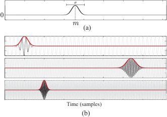
Figure 25: (a) The Gaussian window with spreading factor $\sigma$ centered at time instant $m$. (b) Pulses obtained by windowing three different sinusoids with Gaussian windows of different spread and applied at different time instants.

Let us now construct the atoms of the Gabor dictionary. Recall that in the case of the signal representation in terms of the DFT in (71), each frequency is represented only once, by the corresponding sampled sinusoid, (72). In the Gabor transform, each frequency appears $l$ times; the corresponding sampled sinusoid is multiplied by the Gaussian window sequence, each time shifted by one sample. Thus, at the $i$th frequency bin, we have $l$ atoms, $\bm{g}^{(m,i)},m=0,1,\ldots,l-1$, with elements given by

$$g^{(m,i)}(n)=g(n-m)\psi_{i}(n),\quad n,m,i=0,1,\ldots,l-1,$$ (90)

where $\psi_{i}(n)$ is the $n$th element of the vector $\bm{\psi}_{i}$ in (72). This results to an overcomplete dictionary comprising $l^{2}$ atoms in the $l$-dimensional space. Fig. 25b illustrates the effect of multiplying different sinusoids with Gaussian pulses of different spread and at different time delays. Fig. 26 is a graphical interpretation of the atoms involved in the Gabor dictionary. Each node, $(m,i)$, in this time-frequency plot, corresponds to an atom of frequency equal to $\frac{2\pi}{lT}i$ and delay equal to $m$.

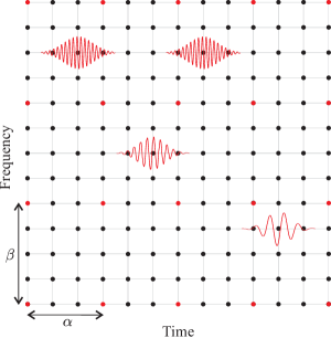
Figure 26: Each atom of the Gabor dictionary corresponds to a node in the time-frequency grid. That is, it is a sampled windowed sinusoid whose frequency and location in time are given by the coordinates of the respective node. In practice, this grid may be subsampled by factors $\alpha$ and $\beta$ for the two axes respectively, in order to reduce the number of the involved atoms.

Note that the windowing of a signal of finite duration inevitably introduces boundary effects, especially when the delay $m$ gets close to the time segment edges, $0$ and $l-1$. A solution to it, that facilitates the theoretical analysis, is to use a modulo $l$ arithmetic to wrap around at the edge points (this is equivalent with extending the signal periodically), see, e.g., [Stro 98].

Once the atoms have been defined, they can be stacked one next to the other to form the columns of the $l\times l^{2}$ Gabor dictionary, $G$. It can be shown that the Gabor dictionary is a tight frame, [Zibu 94].

15.0.2 Time-Frequency Resolution

By the definition of the Gabor dictionary, it is readily understood that the choice of the window spread, as measured by $\sigma$, must be a critical factor, since it controls the localization in time. As it is known from our Fourier transform basics, when the pulse becomes short, in order to increase the time resolution, its corresponding frequency content spreads out, and vice versa. From Heisenberg’s principle, we know that we can never achieve high time and frequency resolution, simultaneously; one is gained at the expense of the other. It is here where the Gaussian shape in the Gabor transform is justified. It can be shown that the Gaussian window gives the optimal trade-off between time and frequency resolution, [Mall 08, Flan 99]. The time-frequency resolution trade-off is demonstrated in Fig. 27, where three sinusoids are shown windowed with different pulse durations. The diagram shows the corresponding spread in the time-frequency plot. The value of $\sigma_{t}$ indicates the time spread and $\sigma_{f}$ the spread of the respective frequency content around the basic frequency of each sinusoid.

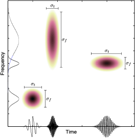
Figure 27: The shorter the width of the pulsed (windowed) sinusoid is in time the wider the spread of its frequency content around the frequency of the sinusoid. The Gaussian-like curves along the frequency axis indicate the energy spread in frequency of the respective pulses. The values of $\sigma_{t}$ and $\sigma_{f}$ indicate the spread in time and frequency, respectively.

15.0.3 Gabor Frames

In practice, $l^{2}$ can take large values and it is desirable to see whether one can reduce the number of the involved atoms, without sacrificing the frame-related properties. This can be achieved by an appropriate subsampling, as this is illustrated in Fig. 26. We only keep the atoms that correspond to the red nodes. That is, we subsample by keeping every $\alpha$ nodes in time and every $\beta$ nodes in frequency in order to form the dictionary, i.e.,

$$G_{(\alpha,\beta)}=\{\bm{g}^{(m\alpha,i\beta)}\},\quad m=0,1,\ldots,\frac{l}{\alpha}-1,\ i=0,1,\ldots,\frac{l}{\beta}-1,$$

where $\alpha$ and $\beta$ are divisors of $l$. Then, it can be shown, e.g., ([Flan 99]), that if $\alpha\beta<l$ the resulting dictionary retains its frame properties. Once $G_{(\alpha,\beta)}$ is obtained, the canonical dual frame is readily available via (79) (adjusted for complex data), from which the corresponding set of expansion coefficients, $\bm{\theta}$, results.

15.0.4 Time-Frequency Analysis of Echolocation Signals Emitted by Bats

Bats are using echolocation for navigation (flying around at night), for prey detection (small insects) and for prey approaching and catching; each bat adaptively changes the shape and frequency content of its calls in order to better serve the previous tasks. Echolocation is used in a similar way for sonars. Bats emit calls as they fly, and “listen” to the returning echoes in order to build up a sonic map of their surroundings. In this way, bats can infer on the distance, the size of obstacles as well as of other flying creatures/insects. Moreover, all bats emit special types of calls, called social calls, which are used for socializing, flirting, etc. The fundamental characteristics of the echolocation calls, as for example, the frequency range and the average time duration, differ from species to species since, thanks to evolution, bats have adapted their calls in order to get best suited to the environment in which a species operates.

Time-Frequency analysis of echolocation calls provides information about the species (species identification) as well as of the specific task and behaviour of the bats in certain environments. Moreover, the bat-biosonar system is studied in order humans to learn more about nature and be inspired for subsequent advances in applications such as sonar navigation systems, radars, medical ultrasonic devices, etc.

Fig. 28a shows a case of a recorded echolocation signal from bats. Zooming at two different parts of the signal, we can observe that the frequency is changing with time. In Fig. 28b, the DFT of the signal is shown, but there is no much information that can be drawn from it, except that the signal is compressible in the frequency domain; most of the activity takes place within a short range of frequencies.

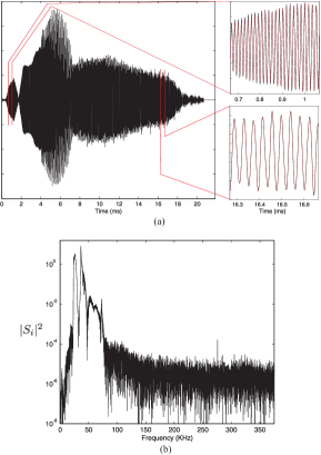
Figure 28: (a) The recorded echolocation signal. The frequency of the signal is time varying and this is indicated by focussing on two different parts of the signal. (b) Plot of the energy of the DFT transform coefficients, $S_{i}$. Observe that most of the frequency activity takes place within a short frequency range.

Our echolocation signal was a recording of total length $T=21.845\text{msecs}$, [Kops 10]. Samples were taken at the sampling frequency $f_{s}=750$ KHz, which results in a total of $l=16384$ samples. Although the signal itself is not sparse in the time domain, we will take advantage of the fact that it is sparse in a transformed domain. We will assume that the signal is sparse in its expansion in terms of the Gabor dictionary.

Our goal in this example is to demonstrate that one does not really need all 16384 samples to perform time-frequency analysis; all the processing can be carried out by using a reduced number of measurements, by exploiting the theory of compressed sensing. To form the measurements vector, $\bm{y}$, the number of measurements was chosen to be $N=2048$. This amounts to a reduction of eight times with respect to the number of available samples. The measurements vector was formed as

$$\bm{y}=X\bm{s},$$

where $X$ is a $N\times l$ sensing matrix comprising $\pm 1$ generated in a random way. This means that once we obtain $\bm{y}$, one does not need to store the original samples any more, leading to a saving in memory. Ideally, one could have obtained the reduced number of measurements by sampling directly the analogue signal at sub-Nyquist rates, as it has already been discussed at the end of Section 10. Another goal is to use both the analysis and synthesis models and demonstrate their difference.

Three different spectrograms were computed. Two of them, shown in Figs. 29b and 29c, correspond to the reconstructed signals obtained by the analysis, (88), and the synthesis, (44), formulations, respectively. In both cases, the NESTA algorithm was used and the $G_{(128,64)}$ frame was employed. Note that the latter dictionary is redundant by a factor of 2. The spectrograms are the result of plotting the time-frequency grid and colouring each node $(t,i)$ according to the energy $|\theta|^{2}$ of the coefficient associated with the respective atom in the Gabor dictionary. The full Gabor transform applied on the reconstructed signals to obtain the spectrograms, in order to get a better coverage of the time-frequency grid. The scale is logarithmic and the darker areas correspond to larger values. The spectrogram of the original signal obtained via the full Gabor transform is shown in Fig. 29d. It is evident, that the analysis model resulted in a more clear spectrogram, which resembles the original one better. When the frame $G_{(64,32)}$ is employed, which is a highly redundant Gabor dictionary comprising $8l$ atoms, then the analysis model results in a recovered signal whose spectrogram is visually indistinguishable from the original one in Fig. 29d.

Fig. 29a is the plot of the magnitude of the corresponding Gabor transform coefficients, sorted in decreasing values. The synthesis model provides a sparser representation, in the sense that the coefficients decrease much faster. The third curve is the one that results if we multiply the dual frame matrix $\tilde{G}_{(128,64)}$ directly with the vector of the original signal samples and it is shown for comparison reasons.

To conclude, the curious reader may wonder what do these curves in Fig. 29d mean after all. The call denoted by (A) belongs to a Pipistrellus pipistrellus (!) and the call denoted by (B) is either a social call or belongs to a different species. The (C) is the return echo from the signal (A). The large spread in time of (C) indicates a highly reflective environment, [Kops 10].

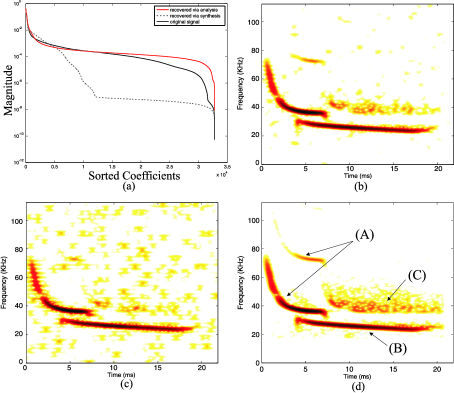
Figure 29: (a) Plot of the magnitude of the coefficients, sorted in decreasing order, in the expansion in terms of the $G_{(128,64)}$ Gabor frame. The results correspond to the analysis and synthesis model formulations. The third curve corresponds to the case of analysing the original vector signal directly, by projecting it on the dual frame. (b) The spectrogram from the analysis and (c) the spectrogram from the synthesis formulations, respectively. (d) The spectrogram corresponding to $G_{(64,32)}$ frame using the analysis formulation. For all cases, the number of measurements used was one eighth of the total number of signal samples. A, B and C indicate different parts of the signal, as explained in the text.

16 From Sparse Vectors to Low Rank Matrices: A highlight

In this section, we move beyond sparse vectors and our goal is to investigate if and how notions related to sparsity can be generalized to matrices. We will see that such a generalization builds upon linear algebra tools and notions related to SVD decomposition, low rank approximation and dimensionality reduction. Our goal is to simply highlight the basic concepts and definitions without delving into a deeper treatment. Our aim is to make the reader alert of the problems and their potential for applications.

16.1 Matrix Completion

Consider a signal vector $\bm{s}\in\mathcal{R}^{l}$, where only $N$ of its components are observed and the rest are unknown. This is equivalent with sensing $\bm{s}$ via a sensing matrix $X$ having its $N$ rows picked uniformly at random from the standard (canonical) basis $\Phi=I$, where $I$ is the $l\times l$ identity matrix. The question which is now posed is whether it is possible to recover the missing components of $\bm{s}$ based on these $N$ components. From the theory presented, so far, we know that one can recover all the components of $\bm{s}$, provided that $\bm{s}$ is sparse in some basis or dictionary, $\Psi$, which exhibits low mutual coherence with $\Phi=I$, and $N$ is large enough, as it has been pointed out in Section 10.

Inspired by the theoretical advances in Compressed Sensing, a question similar in flavor and with a prominent impact regarding practical applications was posed in [Cand 09]. Given a $l_{1}\times l_{2}$ matrix $M$, assume that only $N<<l_{1}l_{2}$ among its entries are known. The question now is whether one is able to recover the exact full matrix. This problem is widely known as matrix completion [Cand 09]. The answer, although it might come as a surprise, is “yes” with high probability, provided that a) the matrix is well structured, b) it has a low rank, $r<<l$, where $l=\min(l_{1},l_{2})$, and c) that $N$ is large enough. Intuitively, this is plausible because a low rank matrix is fully described in terms of a number of parameters (degrees of freedom), which is much smaller than its total number of entries. These parameters are revealed via its Singular Value Decomposition (SVD)

$$M=\sum_{i=1}^{r}\sigma_{i}\bm{u}_{i}\bm{v}_{i}^{T}=U\begin{bmatrix}\sigma_{1}&&\text{\large{0}}\\ &\ddots&&\\ \text{\large{0}}&&\sigma_{r}\end{bmatrix}V^{T},$$ (91)

where $r$ is the rank of the matrix, $\bm{u}_{i}\in\mathcal{R}^{l_{1}}$ and $\bm{v}_{i}\in\mathcal{R}^{l_{2}}$, $i=1,~{}2,\ldots,r$, are the left and right orthonormal singular vectors, spanning the column and row spaces of $M$ respectively, $\sigma_{i}$, $i=1,~{}2,~{},\ldots,~{}r$, are the corresponding singular values and $U=[\bm{u}_{1},\bm{u}_{2},\cdots,\bm{u}_{r}]$, $V=[\bm{v}_{1},\bm{v}_{2},\cdots,\bm{v}_{r}]$.

Let $\bm{\sigma}_{M}$ denote the vector containing all the singular values of $M$, i.e., $\bm{\sigma}_{M}=[\sigma_{1},~{}\sigma_{2},\cdots,\sigma_{l}]^{T}$, then $\operatorname{rank}(M)\coloneqq\left\|{\bm{\sigma}_{M}}\right\|_{0}$. Counting the parameters associated with the singular values and vectors in (91) turns out that the number of degrees of freedom of a rank $r$ matrix is equal to $d_{M}=r(l_{1}+l_{2})-r^{2}$ [Cand 10a]. When $r$ is small, $d_{M}$ is much smaller than $l$.

Let us denote with $\Omega$ the set of $N$ pairs of indexes, $(i,j)$, $i=1,~{},2,\ldots,l_{1}$, $j=1,~{},2,\ldots,l_{2}$, of the locations of the known entries of $M$, which have been sampled uniformly at random. Adopting the main reasoning followed so far, one would attempt to recover $M$ based on the following rank minimization problem

$$\min_{\hat{M}\in\mathcal{R}^{l_{1}\times l_{2}}} \left\|{\bm{\sigma}_{\hat{M}}}\right\|_{0}$$

s.t. $$\hat{M}_{i,j}=M_{i,j},\quad(i,j)\in\Omega.$$ (92)

It turns out that, assuming that there exist a unique low-rank matrix having the specific known entries, then (92) leads to the exact solution [Cand 09]. However, compared to the case of sparse vectors, in the matrix completion problem the uniqueness issue gets much more involved. The following issues play a crucial part concerning the uniqueness of the task in (92).

1. If the number of known entries is lower than the degrees of freedom, i.e., $N<d_{M}$, then there is no way to recover the missing entries whatsoever, since there is an infinite number of low rank matrices consistent with the $N$ observed entries.

2. Even if $N\geq d_{M}$, uniqueness is still not guaranteed. It is required that the $N$ elements with indices in $\Omega$ are such that at least one entry per column and one entry per row is observed. Otherwise, even a rank-1 matrix, i.e, $M=\sigma_{1}\bm{u}_{1}\bm{v}_{1}^{T}$, is not possible to be recovered. This becomes clear with a simple example. Assume that $M$ is a rank-1 matrix and that no entry in the first column as well as in the last row is observed. Then, since for this case $M(i,j)=\sigma_{1}u_{1i}v_{1j}$, it is clear that no information concerning the first component of $\bm{v}_{1}$ as well as the last component of $\bm{u}_{1}$ is available; hence these singular vector components are impossible to be recovered, regardless which method is used. As a consequence, the matrix can not be completed. On the other hand, if the elements of $\Omega$ are picked at random and $N$ is large enough, one can only hope that $\Omega$ is such that to comply with the previous requirement; i.e., at least one entry per row and column is observed, with high probability. It turns out that this problem resembles the famous in probability theory theorem known as the coupon collector’s problem. According to this, at least $N=C_{0}l\ln l$ entries are needed, where $C_{0}$ is a constant [Motw 95]. This is the information theoretic limit for exact matrix completion [Cand 10a] of any low-rank matrix.

3. Even if points (1) and (2) before are fulfilled, still uniqueness is not guaranteed. In fact, not every low rank matrix is liable to exact completion, regardless of the number and the positions of the observed entries. We will demonstrate that with the aid of an example. Let one of the singular vectors be sparse. Assume, without loss of generality, that the third left singular vector, $\bm{u}_{3}$, is sparse with sparsity level $k=1$ and also that its nonzero component is the first one, i.e., $u_{31}\neq 0$. The rest of $\bm{u}_{i}$ and all $\bm{v}_{i}$ are assumed to be dense. Let us return to the SVD for a while, and specifically to the leftmost formula given in (91). Observe that the matrix $M$ is written as the sum of $r$, $l_{1}\times l_{2}$ matrices $\sigma_{i}\bm{u}_{i}\bm{v}_{i}^{T}$, $i=1,\ldots,r$. Thus, in this specific case where $\bm{u}_{3}$ is $k=1$ sparse, the matrix $\sigma_{3}\bm{u}_{3}\bm{v}_{3}^{T}$ has zeros everywhere except from its first row. In other words, the information that $\sigma_{3}\bm{u}_{3}\bm{v}_{3}^{T}$ brings to the formation of $M$ is concentrated to its first row only. This argument can also be viewed from another perspective; the entries of $M$ obtained from any row but the first one, do not provide any useful information with respect to the values of the free parameters $\sigma_{3}$, $\bm{u}_{3}$, $\bm{v}_{3}$. As a result, in this case, unless if one incorporates extra information about the sparse nature of the singular vector, the entries from the first row that are missed are not recoverable, since the number of parameters concerning this row is larger than the available number of data.

   Intuitively, when a matrix has dense singular vectors is better rendered for exact completion, since each one among the observed entries carries information associated with all the $d_{M}$ parameters that fully describe it. To this end, a number of conditions, which evaluate the suitability of the singular vectors, have been established. The simplest one is given next [Cand 09]:

   $$\left\|{\bm{u}_{i}}\right\|_{\infty}\leq\sqrt{\frac{\mu_{B}}{l_{1}}},~{}\left\|{\bm{v}_{i}}\right\|_{\infty}\leq\sqrt{\frac{\mu_{B}}{l_{2}}},~{}i=1,\ldots,r.$$ (93)

   where $\mu_{B}$ is a bound parameter. In fact, $\mu_{B}$ is a measure of the coherence of matrix $U$ (and similarly of $V$),(vis-à-vis the standard basis), defined as follows:

   $$\mu(U)\coloneqq\frac{l_{1}}{r}\max_{1\leq i\leq l_{1}}\left\|{\bm{P}_{U}\bm{e}_{i}}\right\|^{2},$$ (94)

   where $\bm{P}_{U}$ defines the orthogonal projection to subspace $U$ and $\bm{e}_{i}$ is the $i$th vector of the canonical basis. It is easy to show that $\left\|{\bm{P}_{U}\bm{e}_{i}}\right\|^{2}=\left\|{U^{T}\bm{e}_{i}}\right\|^{2}$. In essence, coherence is an index quantifying the extent to which the singular vectors are correlated with the standard basis, $\bm{e}_{i}$, $i=1,2,\ldots,l$. The smaller the $\mu_{B}$ is the less “spiky” the singular vectors are likely to be, and the corresponding matrix is better suited for exact completion. Indeed, assuming for simplicity a square matrix $M$, i.e. $l_{1}=l_{2}=l$, then if any one among the singular vectors is sparse having a single nonzero component only, then, taking into account that $\bm{u}_{i}^{T}\bm{u}_{i}=\bm{v}_{i}^{T}\bm{v}_{i}=1$, this value will have magnitude equal to one and the bound parameter will take its largest value possible, i.e., $\mu_{B}=l$. On the other hand, the smaller value that $\mu_{B}$ can get is $1$, something that occurs when the components of all the singular vectors assume the same value (in magnitude). Note that in this case, due to the normalization, this common component value has magnitude $\frac{1}{l}$. Tighter bounds to the matrix coherence result via the more elaborate incoherence property [Cand 09, Rech 11] and the strong incoherence property [Cand 10a]. In all cases, the larger the bound parameter is the larger the number of known entries, which is required in order to guarantee uniqueness, becomes.

   In section 16.3, the aspects of uniqueness will be discussed in the context of a real life application.

The problem described in (92) is of limited practical interest since it is an NP-hard task. Thus, following the Compressed Sensing paradigm, it is replaced by a convexly relaxed counterpart of it, i.e.,

$$\min_{\hat{M}\in\mathcal{R}^{l_{1}\times l_{2}}} \left\|{\bm{\sigma}_{\hat{M}}}\right\|_{1}$$

s.t. $$\hat{M}_{i,j}=M_{i,j},\quad(i,j)\in\Omega$$ (95)

where $\left\|{\bm{\sigma}_{\hat{M}}}\right\|_{1}$, i.e., the sum of the singular values, is referred to as nuclear norm of the matrix $\hat{M}$, often denoted as $\left\|{\hat{M}}\right\|_{*}$. The nuclear norm minimization was proposed in [Faze 01] as a convex approximation of rank minimization, which can be cast as a semidefinite program.

Theorem 8.

Let $M$ be a $l_{1}\times l_{2}$ matrix of rank $r$, which is a constant much smaller than $l=\max(l_{1},l_{2})$, obeying (93). Suppose that we observe $N$ entries of $M$ with locations sampled uniformly at random. Then there is a positive constant $C$ such that if

$$N\geq C\mu_{B}^{4}l\ln^{2}l,$$ (96)

then $M$ is the unique solution to (95) with probability at leat $1-l^{-3}$.

There might be an ambiguity on how small the rank should be in order for the corresponding matrix to be characterized as “low rank”. More rigorously, a matrix is said to be of low rank if $r=\mathcal{O}(1)$, which means that $r$ is a constant with no dependence (not even logarithmic), on $l$. Matrix completion is also possible for more general rank cases where instead of the mild coherence property of (93), the incoherence and the strong incoherence properties [Cand 09, Cand 10a, Rech 11, Gros 11] are mobilized in order to get similar theoretical guaranties. The detailed exposition of these alternatives is out of the scope of this paper. In fact, Theorem 8 embodies the essence of the matrix completion task: with high probability, nuclear-norm minimization recovers all the entries of a low rank matrix $M$ with no error. More importantly, the number of entries $N$, which the convexly relaxed problem requires, is only by a logarithmic factor larger than the information theoretic limit; recall that the latter is equal to $C_{0}l\ln l$. Moreover, similarly to Compressed Sensing, robust matrix completion in the present of noise is also possible as long as the request $\hat{M}_{i,j}=M_{i,j}$ in (92) and (95) is replaced by $\left\|{\hat{M}_{i,j}-M_{i,j}}\right\|_{2}\leq\epsilon$ [Cand 10b]. Furthermore, the notion of matrix completion has also been extended to tensors [Gand 11, Sign 11].

16.2 Robust PCA

The developments on matrix completion theory led, more recently, to the formulation and solution of another problem of high significance. To this end, the notation $\left\|{M}\right\|_{1}$, i.e., the $\ell_{1}$ norm of a matrix, is introduced and it is defined as the sum of the absolute values of its entries, i.e., $\left\|{M}\right\|_{1}=\sum_{i=1}^{l_{1}}\sum_{j=1}^{l_{2}}|M_{i,j}|$. In other words, it acts on the matrix as if this were a long vector. Assume that $M$ is expressed as the sum of a low rank matrix, $L$, and a sparse matrix, $S$, i.e., $M=L+S$. The following convex minimization problem [Cand 11b, Wrig 09a, Chan 11], usually referred to as principal component pursuit (PCP),

$$\min_{\hat{L}\in\mathcal{R}^{l_{1}\times l_{2}},~{}\hat{S}\in\mathcal{R}^{l_{1}\times l_{2}}} \left\|{\bm{\sigma}_{M}}\right\|_{1}+\lambda\left\|{S}\right\|_{1}$$

s.t. $$\hat{L}+\hat{S}=M,$$ (97)

is shown to recover both $L$ and $S$ according to the following theorem [Cand 11b]:

Theorem 9.

The PCP recovers both $L$ and $S$ with probability at least $1-cl_{1}^{-10}$, where $c$ is a constant, provided that:

1. the support set $\Omega$ of $S$ is uniformly distributed among all sets of cardinality $N$,

2. the number, $k$, of nonzero entries of $S$ is relatively small, i.e., $k\leq\rho l_{1}l_{2}$, where $\rho$ is a sufficiently small positive constant,

3. $L$ obeys the incoherence property,

4. the regularization parameter, $\lambda$, is constant with value $\lambda=\frac{1}{\sqrt{l_{2}}}$,

5. $\operatorname{rank}(L)\leq C\frac{l_{2}}{\ln^{2}l_{1}}$, with $C$ being a constant.

In other words, based on all the entries of a matrix $M$, which is known that is the sum of two unknown matrices $L$ and $S$, with the first one being of low rank matrix and the second being sparse, then PCP recovers exactly, with probability almost 1, both $L$ and $S$, irrespective of how large the magnitude of the entries of $S$ are, provided that both $r$ and $k$ are sufficiently small.

The applicability of the previous task is very broad. For example, PCP can be employed in order to find a low rank approximation of $M$. It is well known that the task of low rank approximation is closely related to the dimensionality reduction task, where the columns of $M$ are expressed in terms of the $r$ (principal components) columns of $U$, e.g., Chapter 6, [Theo 09]. However, in contrast to the standard SVD or PCA approach, PCP is robust and insensitive to the presence of outliers, since these are naturally modeled, via the presence of $S$. For this reason, the above task is widely known as robust PCA via nuclear norm minimization. (More classical PCA techniques are known to be sensitive to outliers and a number of alternative approaches have in the past been proposed towards its robustification, e.g., [Karh 95, Xu 95, Torr 03, Hube 04, Hube 05]).

When PCP serves as a robust PCA approach, the matrix of interest is $L$ and $S$ accounts for the outliers. However, PCP provides estimates for both $L$ and $S$. As it will be discussed in the next subsection, state-of-the-art applications are well accommodated when the focus of interest is turned into the sparse matrix $S$ itself.

Remarks 13.

• Just as $\ell_{1}$ -minimization is the tightest convex relaxation of the combinatorial $\ell_{0}$-minimization problem in compressed sensing, the nuclear-norm minimization is the tightest convex relaxation of the NP-hard rank minimization problem; i.e., the nuclear ball $\{M\in\mathcal{R}^{l_{1}\times l_{2}}:\left\|{M}\right\|_{*}\leq 1\}$ is the convex hull of the set of rank-one matrices with spectral norm bounded by one. Besides the Nuclear norm, other heuristics have also been proposed, such as the log-det heuristic [Faze 04] and the max-norm [Foyg 11].

• The nuclear norm, as a rank minimization approach, is the generalization of the trace-related cost, which is often used in the control community for the rank minimization of positive semidefinite matrices [Mesb 97]. Indeed, when the matrix is symmetric and positive semidefinite, the nuclear norm of $M$ is the sum of the eigenvalues and thus it is equal to the trace of $M$. Such problems arise when, for example, the rank minimization task refers to covariance matrices and positive semidefinite Toeplitz or Hankel matrices (see, e.g., [Faze 04]).

• Both matrix completion (95) and PCP (97) can be formulated as semidefinite programs and are solved via mobilizing interior-point methods. However, whenever the size of a matrix becomes large (e.g., $100\times 100$), these methods are deemed to fail in practice due to excessive power and memory requirements. As a result, there is an increasing interest, which has propelled intensive research efforts, for the development of efficient methods to solve (95), (97) or related approximations, which scale well with large matrices. Many of these methods revolve around the philosophy of the iterative soft and hard thresholding techniques, as discussed in previous sections. However, in the current low rank approximation setting, it is the singular values of the estimated matrix which are thresholded. As a result, in each iteration, the estimated matrix, after thresholding its singular values, tends to be of lower rank. The thesholding of the singular values is either imposed, such as in the case of the singular value thresholding (SVT) algorithm [Cai 10] or it results as a solution of the regularized versions of (95) and (97) (see, e.g., [Toh 10, Chen 11, Lin 10, Gane 09, Yuan 09]). Moreover, algorithms inspired by greedy methods such as CoSaMP, have also been proposed [Lee 10, Wate 11].

• Further developments on robust PCA led to improved versions [Gane 10] allowing for exact recovery even though the number of nonzero entries of $S$ approaches $l_{1}l_{2}$ arbitrarily close, provided that the sign pattern of $S$ is random. Furthermore, even full columns are allowed to be corrupted [Xu 12, McCo 11]. Moreover, fusions of PCP with matrix completion and Compressed Sensing are possible, in the sense that only a subset of the entries of $M$ is available and/or linear measurements of the matrix in a Compressed Sensing fashion can be used instead of matrix entries (see, e.g., [Wate 11, Wrig 12]). Moreover, stable versions of PCP dealing with noise have also been investigated (see, e.g., [Zhou 10]).

16.3 Applications of Matrix Completion and PCP

The number of applications in which these techniques are involved is ever increasing and their extensive presentation is out of the scope of this paper. Next, some key applications will be selectively discussed since they reveal the potential of these methods and at the same time will assist the reader for a better understanding of the underline notions.

16.3.1 Matrix Completion

A typical application, where the matrix completion problem arises, is in the collaborative filtering task [Su 09], which is essential for building up successful recommender systems. Let us consider that a group of individuals provide their ratings concerning products, which they have enjoyed. Then a matrix with ratings can be filled where each row indexes a different individual and the columns index the products. As a popular example take the case where the products are different movies. Inevitably, the associated matrix will be partially filled, since it is not common that all customers have watched all the movies and submit ratings for all of them. Matrix completion comes to provide an answer, potentially in the affirmative, to the following question. Can we predict the ratings that the users would give to films that they have not seen yet? This is the task of a recommender system in order to encourage users to watch movies, which are likely to be of their preference. The exact objective of competition for the famous Netflix prize (http://www.netflixprize.com/) was the development of such a recommender system.

The aforementioned problem provides a good opportunity to build up our intuition about the matrix completion task. Fist, an individual’s preferences or taste on movies are typically governed by a small number of factors, such as the gender, the actors they play in it, the continent of origin, etc. As a result, a matrix fully filled with ratings is expected to be low rank. Moreover, it is clear that each user need to have at least one movie rated in order to have any hope to fill out his/her ratings across all movies. The same is true for each movie. This requirement complies with the second requirement in section 16.1, concerning uniqueness, i.e., one needs to know at least one entry per row and column. Finally, imagine a single user who rates movies with criteria that are completely different to those used by the rest of the users. He/She could, for example, provide ratings at random or depending on, let us say, the first letter of the movie title. Such a scenario complies with the third point concerning the uniqueness in the matrix completion problem, as previously discussed. Unless all the ratings of the specific user are known, the matrix cannot get fully completed.

In the previous application, the matrix of interest can be characterized as approximately low rank. In other cases, such as in sensor network localization [Mao 07], the rank of the matrix assumes an exact value. The goal of localization is to assign geographic coordinates to each node in the sensor network based on a square matrix, which contains the pairwise distances between the nodes [Bisw 06, Mont 10]. It turns out that this matrix is of very low rank, e.g., two or three, depending on whether the sensors are placed in the 2D or 3D space. As a result, matrix completion is possible using a limited number of distance measurements. The number of distance measurements is reduced either intentionally, in order to save power and/or due to the presence of irregularities and obstacles in the deployment area, which renders the communication among nodes impossible. Other applications of matrix completion includes system identification [Liu 10], recovering structure from motion [Chen 04] and multi-task learning [Argy 07].

16.3.2 Robust PCA/PCP

In the collaborative filtering task, robust PCA offers an extra attribute compared to matrix completion, which can be proved very crucial in practice. The users are allowed to even tamper with some of the ratings without affecting the estimation of the low rank matrix. This seems to be the case whenever the rating process involves many individuals in an environment, which is not strictly controlled, since some of them occasionally are expected to provide ratings in an ad-hoc, or even malicious manner.

One of the first applications of PCP was in video surveillance systems [Cand 11b] and the main idea behind it appeared to be popular and extendable to a number of computer vision applications. Take the example of a camera recording a sequence of frames consisting of a merely static background and a foreground with few moving objects, e.g., vehicles and/or individuals. A common task in surveillance video is to extract from the background the foreground, in order, for example, to detect any activity or to proceed with further processing such as face recognition. Suppose the successive frames are converted to vectors in lexicographic order and then are placed as columns in a matrix $M$. Due to the background, even though this may slightly vary due to changes in illumination, successive columns are expected to be highly correlated. As a result, the background can be modeled as an approximately low rank matrix $L$. On the other hand, the objects on the foreground, appear as “anomalies” concerning a fraction of pixels of each frame, i.e., a limited number of entries in each column of $M$. Moreover, due to the motion of the forground objects, the positions of these anomalies are likely to change from one column of $M$ to the next. Therefore, they can be modeled as a sparse matrix $S$. Note that in this application, the matrix of interest is the sparse matrix rather than the low rank one.

17 Conclusions

In this paper, we provided an overview of the major theoretical advances as well as the main trends in algorithmic developments in the area of sparsity-aware learning and compressed sensing. Both batch processing and online processing techniques were considered. A case study in the context of time-frequency analysis of signals was also presented. Our intent is to update the review from time to time, since this is a very hot research area with a momentum and speed that is sometimes difficult to follow up.

Appendix A Appendix

The stage of our discussion in this Appendix is the real Euclidean space $\mathcal{R}^{l}$, where $l$ is a positive integer. Although all of the following arguments hold true even in the case where the $\mathcal{R}^{l}$ is substituted by the much more general Hilbert space setting, we confine ourselves here, for the sake of simplicity, to the Euclidean space. Henceforth, the space $\mathcal{R}^{l}$ is considered to be equipped with an inner product, which, in the present context, is denoted by $\left\langle{\bm{\theta}_{1}},{\bm{\theta}_{2}}\right\rangle$, $\forall\bm{\theta}_{1},\bm{\theta}_{2}\in\mathcal{R}^{l}$. A standard example of such an inner product is the classical vector/dot one, defined by $\left\langle{\bm{\theta}_{1}},{\bm{\theta}_{2}}\right\rangle\coloneqq\bm{\theta}_{1}^{T}\bm{\theta}_{2}$, $\forall\bm{\theta}_{1},\bm{\theta}_{2}\in\mathcal{R}^{l}$, where the superscript $(\cdot)^{T}$ stands for vector transposition. Another example of an inner product for the space $\mathcal{R}^{l}$ is the following weighted one; $\left\langle{\bm{\theta}_{1}},{\bm{\theta}_{2}}\right\rangle\coloneqq\bm{\theta}_{1}^{T}W\bm{\theta}_{2}$, $\forall\bm{\theta}_{1},\bm{\theta}_{2}\in\mathcal{R}^{l}$, where $W\in\mathcal{R}^{l\times l}$ is any user-defined positive definite matrix. In order not to spare the generality of the following discussion, we let $\left\langle{\cdot},{\cdot}\right\rangle$ stand for any user-defined inner product on the linear space $\mathcal{R}^{l}$. Given such an inner product, the associated norm is induced according to the following rule: $\left\|{\cdot}\right\|\coloneqq\sqrt{\left\langle{\cdot},{\cdot}\right\rangle}$. Excellent resources for a deeper study on the extremely rich subject of convex analysis are [Rock 70, Rock 04, Hiri 01, Baus 11].

We start, now, with few notions of fundamental importance to convex analysis.

A.1 Closed convex sets and metric projection mappings

Definition 7 (Convex set, convex function).

A non-empty subset $C$ of $\mathcal{R}^{l}$ is called convex if $\forall\bm{\theta}_{1},\bm{\theta}_{2}\in\mathcal{R}^{l}$, and $\forall\lambda\in[0,1]$, the following holds true: $\lambda\bm{\theta}_{1}+(1-\lambda)\bm{\theta}_{2}\in C$.

Moreover, a function $\mathcal{L}:\mathcal{R}^{l}\rightarrow\mathcal{R}$ is called convex if $\forall\bm{\theta}_{1},\bm{\theta}_{2}\in\mathcal{R}^{l}$, and $\forall\lambda\in[0,1]$, $\mathcal{L}(\lambda\bm{\theta}_{1}+(1-\lambda)\bm{\theta}_{2})\leq\lambda\mathcal{L}(\bm{\theta}_{1})+(1-\lambda)\mathcal{L}(\bm{\theta}_{2})$. The function $\mathcal{L}$ is called strictly convex if $\forall\lambda\in(0,1)$ and $\forall\bm{\theta}_{1},\bm{\theta}_{2}\in\mathcal{R}^{l}$, such that $\bm{\theta}_{1}\neq\bm{\theta}_{2}$, we have $\mathcal{L}(\lambda\bm{\theta}_{1}+(1-\lambda)\bm{\theta}_{2})<\lambda\mathcal{L}(\bm{\theta}_{1})+(1-\lambda)\mathcal{L}(\bm{\theta}_{2})$.

The epigraph of a function $\mathcal{L}$ is defined as the set

$$\operatorname{epi}(\mathcal{L})\coloneqq\bigl{\{}(\bm{\theta},r)\in\mathcal{R}^{l}\times\mathcal{R}:\mathcal{L}(\bm{\theta})\leq r\bigr{\}}.$$

In other words, the epigraph of $\mathcal{L}$ is the set of all points of $\mathcal{R}^{l}\times\mathcal{R}$ which belong to and lie above the graph of $\mathcal{L}$. Notice, also, by the definition of convexity, that $\mathcal{L}$ is convex if and only if $\operatorname{epi}(\mathcal{L})$ is convex.

Given a real number $\xi$, the lower level set of $\mathcal{L}$ at height $\xi$ is defined as the set

$$\operatorname{lev_{\leq\xi}}(\mathcal{L})\coloneqq\bigl{\{}\bm{\theta}\in\mathcal{R}^{l}:\mathcal{L}(\bm{\theta})\leq\xi\bigr{\}}.$$

For the geometry behind the previous definitions, see Fig. 30.

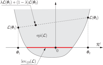
Figure 30: A convex function $\mathcal{L}$, its epigraph, and the lower level set of $\mathcal{L}$ at height $0$.

Definition 8 (The metric projection mapping).

Given a non-empty closed convex set $C\subset\mathcal{R}^{l}$, the metric projection mapping onto $C$ is defined as the operator that maps to each $\bm{\theta}\in\mathcal{R}^{l}$ the unique $P_{C}(\bm{\theta})\in C$ such that

$$\left\|{\bm{\theta}-P_{C}(\bm{\theta})}\right\|=d(\bm{\theta},C).$$

In other words, the point $P_{C}(\bm{\theta})$ is the unique minimizer of the function $\left\|{\bm{\theta}-\bm{x}}\right\|$, $\bm{x}\in C$. Obviously, in the case where $\bm{\theta}\in C$, then $P_{C}(\bm{\theta})=\bm{\theta}$.

As an example, the metric projection mapping onto the hyperslab is given next.

Example 8 (Hyperslab).

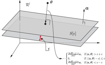
Figure 31: A hyperslab and its associated projection mapping.

A hyperslab $S[\epsilon]$ is the closed convex subset of $\mathcal{R}^{l}$ which is defined as

$$S[\epsilon]\coloneqq\bigl{\{}\bm{x}\in\mathcal{R}^{l}:|\left\langle{\bm{a}},{\bm{x}}\right\rangle-c|\leq\epsilon\bigr{\}},$$

for some nonzero $\bm{a}\in\mathcal{R}^{l}$ and some $c\in\mathcal{R}$. The projection mapping $P_{S[\epsilon]}$ onto $S[\epsilon]$ is given as follows:

$$P_{S[\epsilon]}(\bm{\theta})=\bm{\theta}-\begin{cases}\frac{\left\langle{\bm{a}},{\bm{\theta}}\right\rangle-c-\epsilon}{\left\|{\bm{a}}\right\|^{2}}\bm{a},&\text{if}\left\langle{\bm{a}},{\bm{\theta}}\right\rangle>c+\epsilon,\\ 0,&\text{if}\ |\left\langle{\bm{a}},{\bm{\theta}}\right\rangle-c|\leq\epsilon,\\ \frac{\left\langle{\bm{a}},{\bm{\theta}}\right\rangle-c+\epsilon}{\left\|{\bm{a}}\right\|^{2}}\bm{a},&\text{if}\left\langle{\bm{a}},{\bm{\theta}}\right\rangle<c-\epsilon.\end{cases}$$ (98)

For the related geometry, see Fig. 31. Notice that $\bm{a}$ stands for the normal vector defining the hyperplanes associated with the hyperslab.

A.2 The subgradient

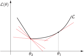
Figure 32: The graph of $\mathcal{L}$ and supporting hyperplanes generated by the subgradients at points, $\theta_{1}$, $\theta_{2}$, where the function is differentiable and non-differentiable, respectively.

Definition 9 (Subgradient, Subdifferential).

Given a convex function $\mathcal{L}$, defined on $\mathcal{R}^{l}$, and a point $\bm{\theta}\in\mathcal{R}^{l}$, the subgradient of $\mathcal{L}$ at $\bm{\theta}$ is defined as any vector, $\bm{h}$, such that

$$\left\langle{\bm{h}},{\bm{x}-\bm{\theta}}\right\rangle+\mathcal{L}(\bm{\theta})\leq\mathcal{L}(\bm{x}),\forall\bm{x}\in\mathcal{R}^{l}.$$ (99)

If the function $\mathcal{L}$ is differentiable at $\bm{\theta}$ then the subgradient coincides with the (unique) gradient. As it is the case for the gradient, a subgradient defines a hyperplane. This hyperplane “supports” the epigraph of $\mathcal{L}$; that is, the epigraph is on the one side of this hyperplane (see Fig. 32). At $\theta_{1}$, the convex function is differentiable and there is only one subgradient, which coincides with the gradient. Thus at this point, there is a simple hyperplane that supports the epigraph. At $\theta_{2}$, the function is not differentiable. Hence there is an infinity of subgradients that define hyperplanes that support the epigraph. The set of all subgradients at a point $\bm{\theta}$ is known as the subdifferential and is denoted as $\partial\mathcal{L}$, i.e.,

$$\partial\mathcal{L}(\bm{\theta})\coloneqq\bigl{\{}\bm{h}\in\mathcal{R}^{l}:\left\langle{\bm{h}},{\bm{x}-\bm{\theta}}\right\rangle+\mathcal{L}(\bm{x})\leq\mathcal{L}(\bm{x}),\forall\bm{x}\in\mathcal{R}^{l}\bigr{\}}.$$

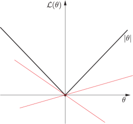
Figure 33: The graph of the function $|\cdot|$, and the supporting hyperplanes generated by the subgradients of $|\cdot|$ at $\theta=0$.

Next, the subdifferential of $\mathcal{L}(\theta)\coloneqq|\theta|$, $\theta\in\mathcal{R}$ is given:

$$\partial\mathcal{L}(\theta)=\begin{cases}[-1,1],&\text{if}\ \theta=0,\\ \operatorname{sgn}(\theta),&\text{if}\ \theta\neq 0,\end{cases}$$

where $\operatorname{sgn}(\cdot)$ stands for the sign of a real number. For the geometry associated to this cost function see Fig. 33.

References

- [Achl 01] Achlioptas D. “Database-friendly random projections”. In: Proceedings of the Symposium on Principles of Database Systems (PODS), pp. 274–281, ACM Press, 2001.
- [Ange 10] Angelosante D., Bazerque J. A., and Giannakis G. B. “Online adaptive estimation of sparse signals: where RLS meets the -norm”. IEEE Trans. Signal Proc., Vol. 58, No. 7, pp. 3436–3447, July 2010.
- [Anto 07] Antoniadis A. “Wavelet methods in statistics: some recent developments and their applications”. Statistics Surveys, Vol. 1, pp. 16–55, 2007.
- [Aren 09] Arenas-Garcia J. and Figueiras-Vidal A. R. “Adaptive combination of proportionate filters for sparse echo cancellation”. IEEE Transactions on Audio, Speech, and Language Processing, Vol. 17, No. 6, pp. 1087–1098, 2009.
- [Argy 07] Argyriou A., Evgeniou T., and Pontil M. “Multi-task feature learning”. In: Advances in Neural Information Processing Systems 19, MIT Press, 2007.
- [Ariy 97] Ariyavisitakul S., Sollenberger N. R., and Greenstein L. J. “Tap-selectable decision feedback equalization”. IEEE Transactions on Communications, Vol. 45, No. 12, pp. 1498–1500, 1997.
- [Asif 10a] Asif M. S. and Romberg J. “Dynamic Updating for minimization”. IEEE Journal of Selected Topics in Signal Processing, Vol. 4, No. 2, pp. 421–434, 2010.
- [Asif 10b] Asif M. S. and Romberg J. “On the LASSO and Dantzig selector equivalence”. In: Conference on Information Sciences and Systems (CISS), Princeton, NJ, March 2010.
- [Bajw 10] Bajwa W. U., Haupt J., Sayeed A. M., and Nowak R. “Compressed Channel Sensing: A New Approach to Estimating Sparse Multipath Channels”. Proceedings of the IEEE, Vol. 98, No. 6, pp. 1058–1076, 2010.
- [Baki 99] Bakin S. Adaptive Regression and Model Selection in Data Mining Problems. PhD thesis, Australian National University, 1999.
- [Bara 08] Baraniuk R. G., Davenport M., DeVore R., and Wakin M. B. “A simple proof of the restricted isometry property for random matrices”. Constructive Approximation, Vol. 28, pp. 253–263, 2008.
- [Bara 09] Baraniuk R. and Wakin M. “Random projections of smooth manifolds”. Foundations of Computational Mathematics, Vol. 9, No. 1, pp. 51–77, 2009.
- [Bara 10a] Baraniuk R., Cevher V., and Wakin M. “Low-dimensional models for dimensionality reduction and signal recovery: A geometric perspective”. Proceedings of the IEEE, Vol. 98, No. 6, pp. 959–971, 2010.
- [Bara 10b] Baraniuk R. G., Cevher V., Duarte M. F., and Hegde C. “Model-based compressive sensing”. IEEE Transactions on Information Theory, Vol. 56, No. 4, pp. 1982–2001, 2010.
- [Baus 11] Bauschke H. H. and Combettes P. L. Convex Analysis and Monotone Operator Theory in Hilbert Spaces. Springer, 2011.
- [Beck 09] Beck A. and Teboulle M. “A fast iterative shrinkage algorithm for linear inverse problems”. SIAM Journal on Imaging Sciences, Vol. 2, No. 1, pp. 183–202, 2009.
- [Beck 11] Becker S., Bobin J., and Candès E. J. “NESTA: A fast and accurate first-order method for sparse recovery”. SIAM Journal on Imaging Sciences, Vol. 4, No. 1, pp. 1–39, 2011.
- [Bene 01] Benesty J., Gansler T., Morgan D. R., Sondhi M. M., and Gay S. L. Advances in Network and Acoustic Echo Cancellation. Springer-Verlag, Berlin, 2001.
- [Berg 08] van den Berg E. and Friedlander M. P. “Probing the pareto frontier for the basis pursuit solutions”. SIAM Journal on Scientific Computing, Vol. 31, No. 2, pp. 890–912, 2008.
- [Bick 09] Bickel P., Ritov Y., and Tsybakov A. “Simultaneous analysis of LASSO and Dantzig selector”. The Annals of Statistics, Vol. 37, No. 4, pp. 1705–1732, 2009.
- [Bisw 06] Biswas P., Liang T.-c., Wang T.-c., and Ye Y. “Semidefinite programming based algorithms for sensor network localization”. ACM Transactions on Sensor Networks, Vol. 2, p. 2006, 2006.
- [Blu 08] Blu T., Dragotti P. L., Vetterli M., Marziliano P., and Coulot L. “Sparse sampling of signal innovations”. IEEE Signal Processing Magazine, Vol. 25, No. 2, pp. 31–40, 2008.
- [Blum 06] Blum A. “Random projection, margins, kernels and feature selection”. In: Lecture Notes on Computer Science (LNCS), pp. 52–68, 2006.
- [Blum 09a] Blumensath T. and Davies M. E. “Iterative hard thresholding for compressed sensing”. Applied and Computational Harmonic Analysis, Vol. 27, No. 3, pp. 265–274, 2009.
- [Blum 09b] Blumensath T. and Davies M. E. “Sampling theorems for signals from the union of finite-dimensional linear subspaces”. IEEE Transactions on Information Theory, Vol. 55, No. 4, pp. 1872–1882, 2009.
- [Blum 10] Blumensath T. and Davies M. E. “Normalized iterative hard thresholding: Guaranteed stability and performance”. IEEE Selected Topics in Signal Processing, Vol. 4, No. 2, pp. 298–309, 2010.
- [Boas 03] Boashash B. Time Frequency Analysis. Elsevier, 2003.
- [Boyd 04] Boyd S. and Vandenberghe L. Convex Optimization. Cambridge University Press, 2004.
- [Bruc 09] Bruckstein A. M., Donoho D. L., and Elad M. “From sparse solutions of systems of equations to sparse modeling of signals and images”. SIAM Review, Vol. 51, No. 1, pp. 34–81, 2009.
- [Cai 09a] Cai J. F., Osher S., and Shen Z. “Split Bregman methods and frame based image restoration”. Multiscale Modeling & Simulation, Vol. 8, No. 2, pp. 337–369, 2009.
- [Cai 09b] Cai T. T., Xu G., and Zhang J. “On recovery of sparse signals via minimization”. IEEE Transactions on Information Theory, Vol. 55, No. 7, pp. 3388–3397, 2009.
- [Cai 10] Cai J.-F., Candès E. J., and Shen Z. “A Singular Value Thresholding Algorithm for Matrix Completion”. SIAM Journal on Optimization, Vol. 20, No. 4, p. 1956, 2010.
- [Cald 09] Calderbank R., Jeafarpour S., and Schapire R. “Compressed learning: Universal spars dimensionality reduction and learning in the measurement domain”. Tech. Rep., Rice University, 2009.
- [Cand 05a] Candès E. J. and Romberg J. “Practical signal recovery from random projections”. In: Proceedings of the SPIE 17th Annual Symposium on Electronic Imaging, Bellingham, WA, 2005.
- [Cand 05b] Candès E. J. and Tao T. “Decoding by linear programming”. IEEE Transactions on Information Theory, Vol. 51, No. 12, pp. 4203–4215, 2005.
- [Cand 06a] Candès E., Romberg J., and Tao T. “Robust uncertainty principles: Exact signal reconstruction from highly incomplete Fourier information”. IEEE Transactions on Information Theory, Vol. 52, No. 2, pp. 489–509, 2006.
- [Cand 06b] Candès E. and Tao T. “Near optimal signal recovery from random projections: Universal encoding strategies”. IEEE Transactions on Information Theory, Vol. 52, No. 12, pp. 5406–5425, 2006.
- [Cand 06c] Candès E. J., Romberg J., and Tao T. “Stable recovery from incomplete and inaccurate measurements”. Communications on Pure and Applied Mathematics, Vol. 59, No. 8, pp. 1207–1223, 2006.
- [Cand 07] Candès E. J. and Tao T. “The Dantzig selector: Statistical estimation when is much larger than ”. Annals of Statistics, Vol. 35, No. 6, pp. 2313–2351, 2007.
- [Cand 08a] Candès E. J. and Wakin M. B. “An Introduction To Compressive Sampling”. Signal Processing Magazine, IEEE, Vol. 25, No. 2, pp. 21–30, march 2008.
- [Cand 08b] Candès E. J., Wakin M. B., and Boyd S. P. “Enhancing sparsity by reweighted minimization”. The Journal of Fourier Analysis and Applications, Vol. 14, No. 5, pp. 877–905, 2008.
- [Cand 09] Candès E. and Recht B. “Exact Matrix Completion via Convex Optimization”. Foundations of Computational Mathematics, Vol. 9, No. 6, pp. 717–772, 2009.
- [Cand 10a] Candès E. and Tao T. “The Power of Convex Relaxation: Near-Optimal Matrix Completion”. Information Theory, IEEE Transactions on, Vol. 56, No. 5, pp. 2053–2080, May 2010.
- [Cand 10b] Candès E. J. and Plan Y. “Matrix Completion With Noise”. Proceedings of the IEEE, Vol. 98, No. 6, pp. 925–936, June 2010.
- [Cand 11a] Candès E. J., Eldar Y. C., Needell D., and Randall P. “Compressed Sensing with Coherent and Redundant Dictionaries”. Applied and Computational Harmonic Analysis, Vol. 31, No. 1, pp. 59–73, 2011.
- [Cand 11b] Candès E. J., Li X., Ma Y., and Wright J. “Robust principal component analysis?”. J. ACM, Vol. 58, No. 3, June 2011.
- [Cevh 09] Cevher V., Indyk P., Hegde C., and Baraniuk R. G. “Recovery of Clustered Sparse Signals from Compressive Measurements”. In: International Conference on Sampling Theory and Applications (SAMPTA), Marseille, France, 2009.
- [Cevh 10] Cevher V., Indyk P., Carin L., and Baraniuk R. G. “Sparse signal recovery and acquisition with graphical models”. IEEE Signal Processing Magazine, Vol. 27, No. 6, pp. 92–103, 2010.
- [Chan 11] Chandrasekaran V., Sanghavi S., Parrilo P. A., and Willsky A. S. “Rank-Sparsity Incoherence for Matrix Decomposition”. SIAM Journal on Optimization, Vol. 21, No. 2, pp. 572–596, 2011.
- [Chen 04] Chen P. and Suter D. “Recovering the missing components in a large noisy low-rank matrix: application to SFM”. IEEE Transactions on Pattern Analysis and Machine Intelligence, Vol. 26, No. 8, pp. 1051 –1063, Aug. 2004.
- [Chen 11] Chen C., He B., and Yuan X. “Matrix completion via an alternating direction method”. IMA Journal of Numerical Analysis, June 2011.
- [Chen 12] Chen F., Chandrakasan A. P., and Stojanovic V. M. “Design and analysis of hardware efficient compressed sensing architectures for compression in wireless sensors”. IEEE Transactions on Solid State Circuits, Vol. 47, No. 3, pp. 744–756, 2012.
- [Chen 98] Chen S., Donoho D. L., and Saunders M. “Atomic decomposition by basis pursuit”. SIAM Journal on Scientific Computing, Vol. 20, No. 1, pp. 33–61, 1998.
- [Clae 73] Claerbout J. F. and Muir F. “Robust modeling with erratic data”. Geophysics, Vol. 38, No. 5, pp. 826–844, 1973.
- [Cohe 09] Cohen A., Dahmen W., and DeVore R. “Compressed sensing and best k-term approximation”. J. Amer. Math. Soc, Vol. 22, No. 1, pp. 211–231, 2009.
- [Coif 92] Coifman R. R. and Wickerhauser M. V. “Entropy-based algorithms for best basis selection”. IEEE Transactions on Information Theory, Vol. 38, No. 2, pp. 713–718, 1992.
- [Comb 05] Combettes P. L. and Wajs V. R. “Signal recovery by proximal forward-backward splitting”. SIAM Journal on Multiscale Modeling and Simulation, Vol. 4, No. 4, pp. 1168–1200, 2005.
- [Comb 11] Combettes P. L. and Pesquet J.-C. “Proximal splitting methods in signal processing”. In: Fixed-Point Algorithms for Inverse Problems in Science and Engineering, Springer-Verlag, 2011.
- [Cott 00] Cotter S. F. and Rao B. D. “Matching pursuit based decision-feedback equalizers”. In: IEEE Conference on Acoustics, Speech and Signal Processing (ICASSP), Istanbul, Turkey, 2000.
- [Dai 09] Dai W. and Milenkovic O. “Subspace Pursuit for Compressive Sensing Signal Reconstruction”. IEEE Transactions on Information Theory, Vol. 55, No. 5, pp. 2230–2249, 2009.
- [Dant 63] Dantzig G. B. Linear Programming and Extensions. Princeton University Press, Princeton, NJn, 1963.
- [Dasg 00] Dasgupta S. “Experiments with random projections”. In: Proceedings of the 16th Conference on Uncertainty in Artificial Intelligence, pp. 143–151, Morgan-Kaufmann, San Francisco, CA, USA, 2000.
- [Daub 04] Daubechies I., Defrise M., and De-Mol C. “An iterative thresholding algorithm for linear inverse problems with a sparsity constraint”. Communications on Pure and Applied Mathematics, Vol. 57, No. 11, pp. 1413–1457, 2004.
- [Daub 10] Daubechies I., DeVore R., Fornasier M., and Güntürk C. S. “Iteratively reweighted least squares minimization for sparse recovery”. Communications on Pure and Applied Mathematics, Vol. 63, No. 1, pp. 1–38, Jan. 2010.
- [Daub 86] Daubechies I., Grossman A., and Meyer Y. “Painless nonorthogonal expansions”. Journal of Mathematical Physics, Vol. 27, pp. 1271–1283, 1986.
- [Daub 88] Daubechies I. “Time-frequency localization operators: A geometric phase space approach”. IEEE Transactions on Information Theory, Vol. 34, No. 4, pp. 605–612, 1988.
- [Dave 10] Davenport M. A. and Wakin M. B. “Analysis of Orthogonal Matching Pursuit Using the Restricted Isometry Property”. IEEE Transactions on Information Theory, Vol. 56, No. 9, pp. 4395–4401, 2010.
- [DeVo 96] DeVore R. A. and Temlyakov V. N. “Some remarks on greedy algorithms”. Advances in Computational Mathematics, Vol. 5, pp. 173–187, 1996.
- [Dono 01] Donoho D. L. and Huo X. “Uncertainty Principles and Ideal Atomic Decomposition”. IEEE Transactions on Information Theory, Vol. 47, No. 7, pp. 2845–2862, 2001.
- [Dono 03] Donoho D. L. and Elad M. “Optimally sparse representation in general (nonorthogonal) dictionaries via minimization”. In: Proceedings of National Academy of Sciences, pp. 2197–2202, 2003.
- [Dono 05] Donoho D. L. and Tanner J. “Neiborliness of randomly-projected simplicies in high dimensions”. In: Proceedings on National Academy of Sciences, pp. 9446–9451, 2005.
- [Dono 06] Donoho D. L. and Tanner J. “Counting faces of randomly projected polytopes when the projection radically lowers dimension”. Tech. Rep. 2006-11, Stanford University, 2006.
- [Dono 10a] Donoho D. L. and J. T. “Counting the faces of randomly projected hypercubes and orthants, wiht applications”. Discrete Computational Geometry, Vol. 43, No. 3, pp. 522–541, 2010.
- [Dono 10b] Donoho D. L. and J. T. “Precise undersampling theorems”. Proceedings of the IEEE, Vol. 98, No. 6, pp. 913–924, 2010.
- [Dono 92] Donoho D. L. and Logan B. F. “Signal recovery and the large sieve”. SIAM Journal on Applied Mathematics, Vol. 52, No. 2, pp. 577–591, 1992.
- [Dono 94] Donoho D. L. and Johnstone I. M. “Ideal spatial adaptation by wavelet shrinkage”. Biometrika, Vol. 81, No. 3, pp. 425–455, 1994.
- [Dono 95] Donoho D., Johnstone I., Kerkyacharian G., and Picard D. “Wavelet Shrinkage: Asymptopia?”. Journal of the Royal Statistical Society, Ser. B, Vol. 57, pp. 301–337, 1995.
- [Drag 07] Dragotti P. L., Vetterli M., and Blu T. “Sampling moments and reconstructing signals of finite rate of innovation: Shannon meets Strang-Fix”. IEEE Transactions on Signal Processing, Vol. 55, No. 5, pp. 1741–1757, 2007.
- [Duar 11] Duarte M. F. and Eldar Y. “Structured Compressed Sensing: From Theory to Applications”. IEEE Transactions on Signal Processing, Vol. 59, No. 9, pp. 4053–4085, 2011.
- [Duar 12] Duarte M. F. and Baraniuk R. G. “Kronecker Compressive Sensing”. IEEE Transactions on Image Processing, Vol. 21, No. 2, pp. 494–504, 2012.
- [Duch 08] Duchi J., Shwartz S. S., Singer Y., and Chandra T. “Efficient projections onto the -ball for learning in high dimensions”. In: Proceedings of the International Conference on Machine Leaning (ICML), pp. 272–279, 2008.
- [Duff 52] Duffin R. J. and Schaeffer A. C. “A class of nonharmonic Fourier series”. Transactions of American Mathematical Society, Vol. 72, pp. 341–366, 1952.
- [Efro 04] Efron B., Hastie T., Johnstone I. M., and Tibshirani R. “Least angle regression”. Annals of Statistics, Vol. 32, pp. 407–499, 2004.
- [Eiwe 10a] Eiwen D., Taubock G., Hlawatsch F., and Feichtinger H. G. “Group sparsity methods for compressive channel estimation in doubly dispersive multicarrier systems”. In: Proceedings IEEE SPAWC, Marrakech, Morocco, June 2010.
- [Eiwe 10b] Eiwen D., Taubock G., Hlawatsch F., Rauhut H., and Czink N. “Multichannel-compressive estimation of doubly selective channels in MIMO-OFDM systems: Exploiting and enhancing joint sparsity”. In: Proceedings International Conference on Acoustics, Speech and Signal Processing (ICASSP), Dallas, Texas, 2010.
- [Elad 02] Elad M. and Bruckstein A. M. “A generalized uncertainty principle and sparse representations in pairs of basis”. IEEE Transactions on Information Theory, Vol. 48, No. 9, pp. 2558–2567, 2002.
- [Elad 05] Elad M., Starck J. L., Querre P., and Donoho D. L. “Simultaneous cartoon and texture image inpainting using morphological component analysis (MCA)”. Applied and Computational Harmonic Analysis, Vol. 19, pp. 340–358, 2005.
- [Elad 07a] Elad M., Matalon B., and Zibulevsky M. “Coordinate and subspace optimization methods for linear least squares with non-quadratic regularization”. Applied and Computational Harmonic Analysis, Vol. 23, pp. 346–367, 2007.
- [Elad 07b] Elad M., Milanfar P., and Rubinstein R. “Analysis versus synthesis in signal priors”. Inverse Problems, Vol. 23, pp. 947–968, 2007.
- [Elad 10] Elad M. Sparse and Redundant Representations: From Theory to Applications in Signal and Image Processing. Springer, 2010.
- [Elda 10] Eldar Y. C., Kuppinger P., and Bolcskei H. “Block-Sparse Signals: Uncertainty Relations and Efficient Recovery”. IEEE Transactions on Signal Processing, Vol. 58, No. 6, pp. 3042–3054, 2010.
- [Fan 01] Fan J. and Li R. “Variable Selection via nonconcave penalized likelihood and its oracle properties”. Journal of the American Statistical Association, Vol. 96, No. 456, pp. 1348–1360, 2001.
- [Faze 01] Fazel M., Hindi H., and Boyd S. P. “A rank minimization heuristic with application to minimum order system approximation”. In: American Control Conference, 2001. Proceedings of the 2001, pp. 4734–4739, 2001.
- [Faze 04] Fazel M., Hindi H., and Boyd S. “Rank minimization and applications in system theory”. In: American Control Conference, 2004. Proceedings of the 2004, pp. 3273–3278, 2004.
- [Figu 03] Figueiredo M. A. and Nowak R. D. “An EM algorithm for wavelet-based image restoration”. IEEE Transactions on Image Processing, Vol. 12, No. 8, pp. 906–916, 2003.
- [Flan 99] Flandrin P. Time-Frequency/Time-scale analysis. Academic Press, 1999.
- [Fouc 11] Foucart S. “Hard Thresholding pursuit: an algorithm for compressive sensing”. SIAM J. Numerical Analysis, Vol. 49, No. 6, pp. 2543–2563, 2011.
- [Foyg 11] Foygel R. and Srebro N. “Concentration-based guarantees for low-rank matrix reconstruction”. In: 24th Annual Conference on Learning Theory (COLT), 2011.
- [Frie 10] Friedman J., Hastie T., and Tibshirani R. “A note on the group LASSO and a sparse group LASSO”. 2010.
- [Gand 11] Gandy S., Recht B., and Yamada I. “Tensor completion and low-n-rank tensor recovery via convex optimization”. Inverse Problems, Vol. 27, No. 2, Feb. 2011.
- [Gane 09] Ganesh A., Lin Z., Wright J., Wu L., Chen M., and Ma Y. “Fast algorithms for recovering a corrupted low-rank matrix”. In: 2009 3rd IEEE International Workshop on Computational Advances in Multi-Sensor Adaptive Processing (CAMSAP), pp. 213–216, Dec. 2009.
- [Gane 10] Ganesh A., Wright J., Li X., Candès E. J., and Ma Y. “Dense error correction for low-rank matrices via principal component pursuit”. In: Information Theory Proceedings (ISIT), 2010 IEEE International Symposium on, pp. 1513–1517, 2010.
- [Garr 08] Garrigues P. J. and Olshausen B. “Learning Horizontal Connections in a Sparse Coding Model of Natural Images”. In: Advances in Neural Information Processing Systems (NIPS), 2008.
- [Ghos 98] Ghosh M. “Blind decision feedback equalization for terrestrial television receivers”. Proceedings of the IEEE, Vol. 86, No. 10, pp. 2070–2081, 1998.
- [Gilb 05] Gilbert A. C., Muthukrisnan S., and Strauss M. J. “Improved time bounds for near-optimal sparse Fourier representation via sampling”. In: Proceedings of SPIE (Wavelets XI), San Diego, CA, 2005.
- [Gold 09] Goldstein T. and Osher S. “The split Bregman algorithm for regularized problems”. SIAM Journal on Imaging Sciences, Vol. 2, No. 2, pp. 323–343, 2009.
- [Goro 97] Gorodnitsky I. F. and Rao B. D. “Sparse signal reconstruction from limited data using FOCUSS: A re-weighted minimum norm algorithm”. IEEE Transactions on Signal Processing, Vol. 45, No. 3, pp. 600–614, 1997.
- [Grib 03] Gribonval R. and Nielsen M. “Sparse decompositions in unions of bases”. IEEE Transactions on Information Theory, Vol. 49, No. 12, pp. 3320–3325, 2003.
- [Gros 11] Gross D. “Recovering Low-Rank Matrices From Few Coefficients in Any Basis”. IEEE Transactions on Information Theory, Vol. 57, No. 3, pp. 1548–1566, March 2011.
- [Hage 81] Hageman L. and Young D. Applied Iterative Methods. Academic Press, New York, 1981.
- [Hale 07] Hale T., Yin W., and Zhang Y. “A fixed-point continuation method for regularized minimization with applications to compressed sensing”. Tech. Rep. TR07-07, Department of Computational and Applied Mathematics, Rice University, 2007.
- [Han 00] Han D. and Larson D. R. Frames, Bases and Group Representations. American Mathematical Society, Providence, RI, 2000.
- [Haup 10] Haupt J., Bajwa W. U., Raz G., and Nowak R. “Toeplitz Compressed Sensing Matrices with Applications to Sparse Channel Estimation”. IEEE Transactions on Information Theory, Vol. 56, No. 11, pp. 5862–5875, 2010.
- [Hayk 96] Haykin S. Adaptive Filter Theory. Prentice-Hall, New Jersey, 3rd Ed., 1996.
- [Hiri 01] Hiriart-Urruty J. and Lemaréchal C. Fundamentals of Convex Analysis. Grundlehren Text Editions Series, Springer-Verlag, 2001.
- [Hoch 90] Hoch J. C., Stern A. S., Donoho D. L., and Johnstone I. M. “Maximum entropy reconstruction of complex (phase sensitive) spectra”. Journal of Magnetic Resonance, Vol. 86, No. 2, pp. 236–246, 1990.
- [Hube 04] Hubert M. and Engelen S. “Robust PCA and classification in biosciences”. Bioinformatics, Vol. 20, No. 11, pp. 1728–1736, 2004.
- [Hube 05] Hubert M., Rousseeuw P. J., and Vanden Branden K. “ROBPCA: A New Approach to Robust Principal Component Analysis”. Technometrics, Vol. 47, No. 1, pp. 64–79, 2005.
- [Jans 84] Jansson P. A. Deconvolution: Applications in Spectroscopy. Academic Press, New York, 1984.
- [Karh 95] Karhunen J. and Joutsensalo J. “Generalizations of principal component analysis, optimization problems, and neural networks”. Neural Networks, Vol. 8, No. 4, pp. 549 – 562, 1995.
- [Kay 93] Kay S. Statistical Signal Processing. Prentice Hall, 1993.
- [Kim 07] Kim S.-J., Koh K., Lustig M., Boyd S., and Gorinevsky D. “An Interior-Point Method for Large-Scale -Regularized Least Squares”. IEEE Journal of Selected Topics in Signal Processing, Vol. 1, No. 4, pp. 606–617, 2007.
- [King 02] Kingsbury N. G. and Reeves T. H. “Overcomplete image coding using iterative projection-based noise shaping”. In: Proceedings IEEE International Conference on Image Processing (ICIP), pp. 597–600, 2002.
- [Kiro 06] Kirolos S., Laska J. N., Wakin M. B., Duarte M. F., Baron D., Ragheb T., Massoud Y., and Baraniuk R. G. “Analog to information conversion via random demodulation”. In: Proceedings of the IEEE Dallas/CAS Workshop on Design, Applications, Integration and Software, pp. 71–74, Dallas, USA, 2006.
- [Knig 00] Knight K. and Fu W. “Asymptotics for the LASSO-type estimators”. The Annals of Statistics, Vol. 28, No. 5, pp. 1356–1378, 2000.
- [Kops 10] Kopsinis Y., Aboutanios E., Waters D. E., and McLaughlin S. “Time-frequency and advanced frequency estimation techniques for the investigation of bat echolocation calls”. The Journal of the Acoustical Society of America, Vol. 127, No. 2, pp. 1124–1134, 2010.
- [Kops 11a] Kopsinis Y., Slavakis K., and Theodoridis S. “Online sparse system identification and signal reconstruction using projections onto weighted balls”. IEEE Transactions on Signal Processing, Vol. 59, No. 3, pp. 936–952, March 2011.
- [Kops 11b] Kopsinis Y., Slavakis K., Theodoridis S., and McLaughlin S. “Reduced complexity online sparse signal reconstruction using projections onto weighted balls”. In: Digital Signal Processing (DSP), 2011 17th International Conference on, pp. 1–8, july 2011.
- [Kops 12a] Kopsinis Y., Slavakis K., Theodoridis S., and McLaughlin S. 2012. Submitted for publication on ISCASS 2013.
- [Kops 12b] Kopsinis Y., Slavakis K., Theodoridis S., and McLaughlin S. “Generalized thresholding sparsity-aware algorithm for low complexity online learning”. In: Proceedings of the IEEE International Conference on Acoustics, Speech, and Signal Processing (ICASSP), pp. 3277–3280, Kyoto: Japan, March 2012.
- [Kova 07] Kovacevic J. and Chebira A. “Life beyond bases: the advent of frames”. IEEE Signal Processing Magazine, Vol. 24, No. 4, pp. 86–104, 2007.
- [Lang 09] Langford J., Li L., and Zhang T. “Sparse online learning via truncated gradient”. Journal of Machine Learning Research, Vol. 10, pp. 777–801, 2009.
- [Lee 10] Lee K. and Bresler Y. “ADMiRA: Atomic Decomposition for Minimum Rank Approximation”. IEEE Transactions on Information Theory, Vol. 56, No. 9, pp. 4402–4416, Sep. 2010.
- [Lin 10] Lin Z., Chen M., and Ma Y. “The Augmented Lagrange Multiplier Method for Exact Recovery of Corrupted Low-Rank Matrices”. arXiv:1009.5055, Sep. 2010.
- [Lin 98] Lin Y.-P. and Vaidyanathan P. P. “Periodically nonuniform sampling of bandpass signals”. IEEE Transactions on Circuits and Systems II, Vol. 45, No. 3, pp. 340–351, 1998.
- [Liu 10] Liu Z. and Vandenberghe L. “Interior-Point Method for Nuclear Norm Approximation with Application to System Identification”. SIAM Journal on Matrix Analysis and Applications, Vol. 31, No. 3, pp. 1235–1256, 2010.
- [Lu 08a] Lu Y. M. and Do M. N. “Sampling signals from a union of subspaces”. IEEE Signal Processing Magazine, Vol. 25, No. 2, pp. 41–47, 2008.
- [Lu 08b] Lu Y. M. and Do M. N. “A theory for sampling signals from a union of subspaces”. IEEE Transactions on Signal Processing, Vol. 56, No. 6, pp. 2334–2345, 2008.
- [Luo 92] Luo Z. Q. and Tseng P. “On the convergence of the coordinate descent method for convex differentiable minimization”. Journal of Optimization Theory and Applications, Vol. 72, No. 1, pp. 7–35, 1992.
- [Maec 12] Maechler P., Felber N., Kaeslin H., and Burg A. “Hardware-Efficient random sampling of Fourier-sparse signals”. In: Proceedings of the IEEE International Symposium on Circuits and Systems (ISCAS), 2012.
- [Male 10] Maleki A. and Donoho D. L. “Optimally tuned iterative reconstruction algorithms for compressed sensing”. IEEE Journal on selected Topics in Signal Processing, Vol. 4, No. 2, pp. 330–341, 2010.
- [Male 11] Maleki A., Anitori L., Yang Z., and Baraniuk R. “Asymptotic Analysis of Complex LASSO via Complex Approximate Message Passing (CAMP)”. arXiv:1108.0477, submitted to IEEE Transactions on Information Theory, Aug. 2011.
- [Mali 05] Malioutov D. M., Cetin M., and Willsky A. S. “Homotopy continuation for sparse signal representation”. In: IEEE International Conference on Acoustics, Speech and Signal Processing (ICASSP), pp. 733–736, 2005.
- [Mall 08] Mallat S. A Wavelet Tour of Signal Processing: The Sparse Way. Academic Press, 3rd Ed., 2008.
- [Mall 93] Mallat S. and Zhang S. “Matching Pursuit in a time-frequency dictionary”. IEEE Transactions on Signal Processing, Vol. 41, pp. 3397–3415, 1993.
- [Mao 07] Mao G., Fidan B., and Anderson B. D. “Wireless sensor network localization techniques”. Computer Networks, Vol. 51, No. 10, pp. 2529–2553, July 2007.
- [Matu 12] Matusiak E. and Eldar Y. C. “Sub-Nyquist Sampling of Short Pulses”. IEEE Transactions on Signal Processing, Vol. 60, No. 3, pp. 1134–1148, 2012.
- [McCo 11] McCoy M. and Tropp A. J. “Two proposals for robust PCA using semidefinite programming”. Electronic Journal of Statistics, Vol. 5, pp. 1123–1160, 2011. Mathematical Reviews number (MathSciNet): MR2836771.
- [Mend 08] Mendelson S., Pajor A., and Tomczak-Jaegermann N. “Uniform uncertainty principle for Bernoulli and subgaussian ensembles”. Constructive Approximation, Vol. 28, pp. 277–289, 2008.
- [Mesb 97] Mesbahi M. and Papavassilopoulos G. “On the rank minimization problem over a positive semidefinite linear matrix inequality”. IEEE Transactions on Automatic Control, Vol. 42, No. 2, pp. 239–243, Feb. 1997.
- [Mile 10] Mileounis G., Babadi B., Kalouptsidis N., and Tarokh V. “An adaptive greedy algorithm with application to nonlinear communications”. IEEE Transactions on Signal Processing, Vol. 58, No. 6, pp. 2998–3007, 2010.
- [Mish 10] Mishali M., Eldar Y. C., and Elron A. “Xampling: Analog data compression”. In: Proceedings Data Compression Conference, Snowbird, Utah, USA, 2010.
- [Mish 11a] Mishali M. and Eldar Y. C. “Sub-Nyquist sampling”. IEEE Signal Processing Magazine, Vol. 28, No. 6, pp. 98–124, 2011.
- [Mish 11b] Mishali M., Eldar Y. C., and Elron A. “Xampling: Signal Acquisition and Processing in Union of Subspaces”. IEEE Transactions on Signal Processing, Vol. 59, No. 10, pp. 4719–4734, 2011.
- [Mont 10] Montanari A. and Oh S. “On positioning via distributed matrix completion”. In: 2010 IEEE Sensor Array and Multichannel Signal Processing Workshop (SAM), pp. 197–200, Oct. 2010.
- [Motw 95] Motwani R. and Raghavan P. Randomized Algorithms. Cambridge University Press, 1995.
- [Nam 12] Nam S., Davies M. E., Elad M., and Gribonval R. “The cosparse analysis model and algorithms”. 2012. To appear in Applied and Computational Harmonic Analysis.
- [Nata 95] Natarajan B. K. “Sparse approximate solutions to linear systems”. SIAM Journal on Computing, Vol. 24, pp. 227–234, 1995.
- [Nayl 04] Naylor P. A., Cui J., and Brookes M. “Adaptive algorithms for sparse echo cancellation”. Signal Processing, Vol. 86, pp. 1182–1192, 2004.
- [Need 09] Needell D. and Tropp J. A. “COSAMP: Iterative signal recovery from incomplete and inaccurate samples”. Applied and Computational Harmonic Analysis, Vol. 26, No. 3, pp. 301–321, 2009.
- [Need 12] Needell D. and Ward R. “Stable image reconstruction using total variation minimization”. 2012.
- [Nest 83] Nesterov Y. E. “A method for solving the convex programming problem with convergence rate ”. Dokl. Akad. Nauk SSSR, Vol. 269, pp. 543–547, 1983. in Russian.
- [Oboz 06] Obozinski G., Taskar B., and Jordan M. “Multi-task feature selection”. Tech. Rep., Department of Statistics, University of California, Berkeley, 2006.
- [Ogur 02] Ogura N. and Yamada I. “Non-strictly convex minimization over the fixed point set of the asymptotically shrinking nonexpansive mapping”. Numerical Functional Analysis and Optimization, Vol. 23, pp. 113–137, 2002.
- [Osbo 00] Osborne M. R., Presnell B., and Turlach B. A. “A new approach to variable selection in least squares problems”. IMA Journal on Numerical Analysis, Vol. 20, pp. 389–403, 2000.
- [Parv 08] Parvaresh F., Vikalo H., Misra S., and Hassibi B. “Recovering Sparse Signals Using Sparse Measurement Matrices in Compressed DNA Microarrays”. IEEE Journal of Selected Topics in Signal Processing, Vol. 2, No. 3, pp. 275–285, 2008.
- [Pink 89] Pinkus A. M. On -approximation. Vol. 93 of Cambridge Tracts in Mathematics, Cambridge University Press, 1989.
- [Plum 05] Plumbley M. D. “Geometry and homotopy for L1 sparse representation”. In: Proceedings of the International Workshop on Signal Processing with Adaptive Sparse Structured Representations (SPARS), Rennes, France, 2005.
- [Rech 11] Recht B. “A Simpler Approach to Matrix Completion”. J. Mach. Learn. Res., Vol. 12, pp. 3413–3430, Dec. 2011.
- [Rive 09] Rivenson Y. and Stern A. “Compressed imaging with a separable sensing operator”. IEEE Signal Processing Letters, Vol. 16, No. 6, pp. 449–452, 2009.
- [Rock 04] Rockafellar R. T. and Wets R. J.-B. Variational Analysis. Springer, Berlin, 2004.
- [Rock 70] Rockafellar T. R. Convex Analysis. Princeton University Press, Princeton, NJ, 1970.
- [Rock 76] Rockafellar R. T. “Monotone operators and the proximal point algorithms”. SIAM Journal on Control and Optimization, Vol. 14, No. 5, pp. 877–898, 1976.
- [Rond 03] Rondogiannis A. and Berberidis K. “Efficient Decision Feedback Equalization for Sparse Wireless Channels”. IEEE Transactions on Wireless Communications, Vol. 2, No. 3, pp. 570–581, 2003.
- [Rubi 10] Rubinstein R., Bruckstein A., and Elad M. “Dictionaries for Sparse Representation Modeling”. Proceedings of the IEEE, Vol. 98, No. 6, pp. 1045 –1057, June 2010.
- [Rude 08] Rudelson M. and Vershynin R. “On sparse reconstruction from Fourier and Gaussian measurements”. Communications on Pure and Applied Mathematics, Vol. 61, No. 8, pp. 1025–1045, 2008.
- [Rudi 92] Rudin L. I., Osher S., and Fatemi E. “Nonlinear total variation based noise removal algorithms”. Physica D: Nonlinear Phenomena, Vol. 60, No. 1-4, pp. 259–268, 1992.
- [Sant 86] Santosa F. and Symes W. W. “Linear inversion of band limited reflection seismograms”. SIAM Journal of Scientific Computing, Vol. 7, No. 4, pp. 1307–1330, 1986.
- [Saye 03] Sayed A. H. Fundamentals of Adaptive Filtering. John Wiley & Sons, New Jersey, 2003.
- [Sele 09] Selesnick I. W. and Figueiredo M. A. T. “Signal restoration with overcomplete wavelet transforms: Comparison of analysis and synthesis priors”. In: Proceedings of SPIE, 2009.
- [Sign 11] Signoretto M., Van de Plas R., De Moor B., and Suykens J. “Tensor Versus Matrix Completion: A Comparison With Application to Spectral Data”. IEEE Signal Processing Letters, Vol. 18, No. 7, pp. 403–406, July 2011.
- [Slav 06] Slavakis K., Yamada I., and Ogura N. “The adaptive projected subgradient method over the Fixed Point Set of Strongly Attracting Nonexpansive Mappings”. Numerical Functional Analysis and Optimization, Vol. 27, No. 7&8, pp. 905–930, 2006.
- [Spre 11] Sprechmann P., Ramirez I., Sapiro G., and Eldar Y. C. “CHiLasso: A Collaborative Hierarchical Sparse Modeling Framework”. IEEE Transactions on Signal Processing, Vol. 59, No. 9, pp. 4183–4198, 2011.
- [Star 02] Starck J. L., Candès E. J., and Donoho D. L. “The curvelet transform for image denoising”. IEEE Transactions on Image Pocessing, Vol. 11, No. 6, pp. 670–684, 2002.
- [Star 07] Starck J. L., Fadili J., and Murtagh F. “The undecimated wavelet decomposition and its reconstruction”. IEEE Transactions on Signal Processing, Vol. 16, No. 2, pp. 297–309, 2007.
- [Stro 98] Strohmer T. Gabor Analysis and Algorithms: Theory and Applications, Chap. Numerical algorithms for discrete Gabor expansions, pp. 267–294. Birkhauser, Boston, MA, 1998.
- [Su 09] Su X. and Khoshgoftaar T. M. “A survey of collaborative filtering techniques”. Adv. in Artif. Intell., Vol. 2009, pp. 1–19, Jan. 2009.
- [Takh 06] Takhar D., Bansal V., Wakin M., Duarte M., Baron D., Kelly K. F., and Baraniuk R. G. “A compressed sensing camera: New theory and an implementation using digital micromirrors”. In: Proceedings on Computational Imaging (SPIE), San Jose, CA, 2006.
- [Tang 11] Tang G. and Nehorai A. “Performance Analysis of Sparse Recovery Based on Constrained Minimal Singular Values”. IEEE Transactions on Signal Processing, Vol. 59, No. 12, pp. 5734–5745, Dec. 2011.
- [Tayl 79] Taylor H. L., Banks S. C., and McCoy J. F. “Deconvolution with the norm”. Geophysics, Vol. 44, No. 1, pp. 39–52, 1979.
- [Teml 03] Temlyakov V. N. “Nonlinear methods of approximation”. Foundations of Computational Mathematics, Vol. 3, No. 1, pp. 33–107, 2003.
- [Theo 09] Theodoridis S. and Koutroumbas K. Pattern Recognition. Academic Press, 4th Ed., 2009.
- [Theo 11] Theodoridis S., Slavakis K., and Yamada I. “Adaptive Learning in a World of Projections”. Signal Processing Magazine, IEEE, Vol. 28, No. 1, pp. 97–123, Jan. 2011.
- [Tian 07] Tian Z. and Giannakis G. B. “Compressed sensing for wideband cognitive radios”. In: Proceedings of the IEEE Conference on Acoustics, Speech and Signal Processing (ICASSP), pp. 1357–1360, 2007.
- [Tibs 96] Tibshirani R. “Regression shrinkage and selection via the LASSO”. J. Royal. Statist. Soc. B., Vol. 58, No. 1, pp. 267–288, 1996.
- [Toh 10] Toh K. C. and Yun S. “An accelerated proximal gradient algorithm for nuclear norm regularized linear least squares problems”. Pacific Journal of Optimization, Vol. 6, pp. 615–640, 2010.
- [Torr 03] De la Torre F. and Black M. J. “A Framework for Robust Subspace Learning”. International Journal of Computer Vision, Vol. 54, No. 1, pp. 117–142, 2003.
- [Tosi 11] Tosić I. and Frossard P. “Dictionary Learning”. IEEE Signal Processing Magazine, Vol. 28, No. 2, pp. 27 –38, March 2011.
- [Trop 04] Tropp J. A. “Greed is good”. IEEE Transactions on Information Theory, Vol. 50, pp. 2231–2242, 2004.
- [Trop 10] Tropp J. A., Laska J. N., Duarte M. F., Romberg J. K., and Baraniuk G. “Beyond Nyquist: Efficient sampling of sparse bandlimited signals”. IEEE Transactions on Information Theory, Vol. 56, No. 1, pp. 520–544, 2010.
- [Tsai 07] Tsaig Y. Sparse Solution of Underdetermined Linear Systems: Algorithms and Applications. PhD thesis, Stanford University, 2007.
- [Unse 00] Unser M. “Sampling: 50 years after Shannon”. Proceedings of the IEEE, Vol. 88, No. 4, pp. 569–587, 2000.
- [Vaug 91] Vaughan R. G., Scott N. L., and White D. R. “The theory of bandpass sampling”. IEEE Transactions on Signal Processing, Vol. 39, No. 9, pp. 1973–1984, 1991.
- [Venk 00] Venkataramani R. and Bresler Y. “Perfect reconstruction formulas and bounds on aliasing error in sub-Nyquist nonuniform sampling of multiband signals”. IEEE Transactions on Information Theory, Vol. 46, No. 6, pp. 2173–2183, 2000.
- [Vett 02] Vetterli M., Marzilliano P., and Blu T. “Sampling signals with finite rate of innovation”. IEEE Transactions on Signal Processing, Vol. 50, No. 6, pp. 1417–1428, 2002.
- [Waki 08] Wakin M. “Manifold-based signal recovery and parameter estimation from compressive measurements”. 2008. preprint: http://arxiv.org/abs/1002.1247.
- [Wate 11] Waters A. E., Sankaranarayanan A. C., and Baraniuk R. G. “SpaRCS: Recovering low-rank and sparse matrices from compressive measurements”. Proc. Adv. in Neural Processing Systems (NIPS), Granada, Spain, 2011.
- [Welc 74] Welch L. R. “Lower bounds on the maximum cross correlation of signals”. IEEE Transactions on Information Theory, Vol. 20, No. 3, pp. 397–399, 1974.
- [Wrig 09a] Wright J., Peng Y., Ma Y., Ganesh A., and Rao S. “Robust Principal Component Analysis: Exact Recovery of Corrupted Low-Rank Matrices by Convex Optimization”. In: Neural Information Processing Systems (NIPS), 2009.
- [Wrig 09b] Wright S., Nowak R., and Figueiredo M. “Sparse reconstruction by separable approximation”. IEEE Transactions on Signal Processing, Vol. 57, No. 7, pp. 2479–2493, 2009.
- [Wrig 12] Wright J., Ganesh A., Min K., and Ma Y. “Compressive Principal Component Pursuit”. arXiv:1202.4596, Feb. 2012.
- [Xu 12] Xu H., Caramanis C., and Sanghavi S. “Robust PCA via Outlier Pursuit”. IEEE Transactions on Information Theory, Vol. 58, No. 5, pp. 3047–3064, May 2012.
- [Xu 95] Xu L. and Yuille A. “Robust principal component analysis by self-organizing rules based on statistical physics approach”. Neural Networks, IEEE Transactions on, Vol. 6, No. 1, pp. 131 –143, jan 1995.
- [Yagh 09] Yaghoobi M., Daudet L., and Davies M. “Parametric Dictionary Design for Sparse Coding”. IEEE Transactions on Signal Processing, Vol. 57, No. 12, pp. 4800–4810, Dec. 2009.
- [Yama 04] Yamada I. and Ogura N. “Hybrid steepest descent method for variational inequality problem over the fixed point set of certain quasi-nonexpansive mappings”. Numerical Functional Analysis and Optimization, Vol. 25, No. 7&8, pp. 619–655, 2004.
- [Yang 10] Yang J., Zhang Y., and Yin W. “A fast alternating direction method for TV - signal reconstruction from partial Fourier data”. IEEE Transactions on Selected Topics for Signal Processing, Vol. 4, No. 2, pp. 288–297, 2010.
- [Ye 97] Ye Y. Interior Point Methods: Theory and Analysis. Wiley, New York, 1997.
- [Yin 08] Yin W., Osher S., Goldfarb D., and Darbon J. “Bregman iterative algorithms for -minimization with applications to compressed sensing”. SIAM Journal of Imaging Sciences, Vol. 1, No. 1, pp. 143–168, 2008.
- [Yu 08] Yu Z., Hoyos S., and Sadler B. M. “Mixed-signal parallel compressed sensing and reception for cognitive radio”. In: Proceedings IEEE Conference on Acoustics, Speech and Signal Processing (ICASSP), pp. 3861–3864, 2008.
- [Yuan 07] Yuan M. and Lin Y. “Model selection and estimation in regression with grouped variables”. Journal of the Royal Statistical Society, Vol. 68, No. 1, pp. 49–67, 2007.
- [Yuan 09] Yuan X. M. and Yang J. F. “Sparse and low-rank matrix decomposition via alternating direction methods”. Pacific Journal of Optimization, 2009.
- [Zhan 11] Zhang T. “Sparse Recovery With Orthogonal Matching Pursuit Under RIP”. IEEE Transactions on Information Theory, Vol. 57, No. 9, pp. 6215–6221, 2011.
- [Zhou 10] Zhou Z., Li X., Wright J., Candès E., and Ma Y. “Stable principal component pursuit”. In: Information Theory Proceedings (ISIT), 2010 IEEE International Symposium on, pp. 1518–1522, 2010.
- [Zibu 10] Zibulevsky M. and Elad M. “L1-L2 Optimization in Signal Processing”. IEEE Signal Processing Magazine, Vol. 27, No. 3, pp. 76–88, 2010.
- [Zibu 94] Zibulevsky M. and Zeevi Y. Y. “Frame analysis of the discrete Gabor scheme”. IEEE Transactions on Signal Processing, Vol. 42, No. 4, pp. 942–945, 1994.
- [Zou 06] Zou H. “The adaptive LASSO and its oracle properties”. Journal of the American Statistical Association, Vol. 101, pp. 1418–1429, Dec. 2006.
- [Zou 08] Zou H. and Li R. “One-step sparse estimates in nonconcave penalized likelihood models”. The Annals of Statistics, Vol. 36, No. 4, pp. 1509–1533, 2008.