J band Variability of M Dwarfs in the WFCAM Transit Survey

Abstract

We present an analysis of the photometric variability of M dwarfs in the WFCAM Transit Survey. Although periodic lightcurve variability in low mass stars is generally dominated by photospheric star spot activity, M dwarf variability in the $J$ band has not been as thoroughly investigated as at visible wavelengths. Spectral type estimates for a sample of over 200,000 objects are made using spectral type-colour relations, and over 9600 dwarfs ($J$$<$17) with spectral types later than K7 were found. The light curves of the late-type sample are searched for periodicity using a Lomb-Scargle periodogram analysis. A total of 68 periodic variable M dwarfs are found in the sample with periods ranging from 0.16 days to 90.33 days, with amplitudes in the range of $\sim 0.009$ to $\sim 0.115$ in the $J$ band. We simulate active M dwarfs with a range of latitude-independent spot coverages and estimate a periodically variable fractions of 1-3 per cent for stars where spots cover more than 10 per cent of the star’s surface. Our simulated spot distributions indicate that operating in the $J$ band, where spot contrast ratios are minimised, enables variability in only the most active of stars to be detected. These findings affirm the benefits of using the $J$ band for planetary transit searches compared to visible bands. We also serendipitously find a $\Delta$$J$$>$$0.2$ mag flaring event from an M4V star in our sample.

1 Introduction

The number of exoplanet discoveries has been growing at an increasing rate, while the lower mass limit for habitable-zone planets grows increasingly closer to 1M_⊕. Indeed, planets of less than 1M_⊕ orbiting sun-like stars have been recently been detected (Fressin et al., 2011). Recent discoveries by Vogt et al. (2010) and Charbonneau et al. (2009) have highlighted how rich in low mass planets M dwarf systems can be. While radial velocity surveys have been productive in detecting exoplanet M dwarf systems, only seven of the 251 known transiting planets have been detected orbiting M dwarfs, in four systems: GJ 436 (Coughlin et al., 2008; Gillon et al., 2007), GJ 1214 (Charbonneau et al., 2009), KOI 961 (Muirhead et al., 2012), and KOI-254 (Johnson et al., 2012). The Kepler satellite has so far identified more then 30 early M dwarf planetary host star candidates from 2510 stars cooler than 4000K being monitored (Borucki et al., 2011). The Wide Field Camera (WFCAM) Transit Survey (WTS) is a UK Infra-red Telescope (UKIRT) Campaign Survey comprising more than 100 nights worth of observations. Its main science driver is to identify planets orbiting M dwarf stars. The observations comprise four fields, each of which is itself comprised of eight pointings of the of WFCAM, which uses four 2048$\times$2048 pixel imaging arrays each covering 13.65’$\times$13.65’. The most complete field has accumulated a total of 1197 epochs of observations over 5 years. Light curves were obtained in the $J$ band only with single deep exposures in $ZYJFK$ bands. A full description of the observation technique is given by Nefs et al. (2012). Data reduction and light curve production has been carried out by the Cambridge Astronomical Survey Unit (CASU) using a customised pipeline (Irwin et al., 2007; Kovács, G. and Hodgkin, S. and Sipőcz, B and Pinfield, D., and others, 2012). In addition to transit searches the WTS lightcurves facilitate a wide range of additional science, including the search for and study of variable M dwarfs, on which our work is focused. The sampling and overall time base-line of the survey potentially permits sensitivity to periods up to tens of days.

Name	Coordinates	No. of epochs	Objects (J$<$17)
	RA (h), Dec (deg)
19	19.58+36.44	1197	69161
17	17.25+03.74	832	17103
07	07.09+12.94	770	21224
03	03.65+39.23	589	15159

Table 1: A table summarising the properties of the four fields comprising WTS.

Both transit surveys (eg. Berta et al., 2012; Miller et al., 2008) and eclipsing binary studies (eg. Morales et al., 2010) suffer from the intrinsic photometric variability of the target stars which must be constrained and accounted for. A thorough understanding of activity of stars is vital in order to uniformly obtain the parameters of any orbiting planets from both transit and radial velocity surveys, or indeed the thresholds set by activity beyond which it is impossible to detect planets. In this paper we classify a sample of M dwarfs in the WTS survey and search for periodic variability in the long-baseline $J$-band light curves. While we do not intend to directly test for planet parameter retrieval, we aim to corroborate previous surveys of M dwarf variability at shorter wavelengths in the near infra red and parameterise the variability of the sample.

2 M dwarf variability

The periodic variability in M dwarfs can result from the modulation of brightness by cool star spots. M dwarfs, like all stars, enter the main sequence rotating rapidly due to the angular momentum of the cloud from which they form. The rotation induces a dynamo giving rise to magnetic activity in the photosphere that produces stellar spots. For solar-type stars the $\alpha-\Omega$ dynamo generated at the tachocline, the boundary between the convection and radiative zones, (Browning et al., 2010) results in latitude dependent spots from the generation of toroidal fields by differential rotation within the star (Brown et al., 2008) that confine magnetic flux tubes to high latitudes (Moreno-Insertis et al., 1992; Schuessler & Solanki, 1992), and Granzer et al. (2000) find that low latitude magnetic flux emergence can occur in very young, partially radiative, main sequence stars, which could give rise to spots at all latitudes. However, stars later than M3.5 are fully convective, so no tachocline exists at which such a dynamo can be generated, yet stars of a later spectral type are still active and this activity may be dependent on an alternative form of dynamo (Rockenfeller et al., 2006; Brown et al., 2008). This switch over at M3.5 has been confirmed through observations of the magnetic energy of M dwarfs (e.g. Reiners & Basri, 2008). Indeed, spectropolarimetric studies of objects known to be fully convective by Morin et al. (2008, 2010) have found such a switch in magnetic field morphology. An alternative dynamo, ultimately dependent on the Coriolis force and called $\alpha^{2}$, has been shown by Chabrier & Küker (2006) as being the type of dynamo process occurring in fully convective, low mass objects such as late M dwarfs and brown dwarfs. The magnetic field generated by the $\alpha^{2}$ dynamo is quadrupolar. The more distributed field in these models could lead to a more distributed spot pattern. The exact nature of the dynamo process and its dependencies in fully convective M dwarfs is yet to be properly understood, while observations continue to place restraints on future models.

Observations by Barnes et al. (2002) indicate a uniform distribution of star spots at all latitudes for partially radiative stars, while others find spots concentrated in the polar regions (Morales et al., 2010; Jeffers et al., 2007) that more closely resemble model predictions of magnetic activity. Frasca et al. (2009) fit K and M dwarfs light curves of varying morphologies using a variety of models consisting of just two large spots, although they do not consider alternative spot distributions and instead vary the spot latitudes and temperatures, and the stellar inclination. An approximately uniform distribution of spots will also result in a variable light curve due to local over- or under-densities of spots on the star. Photometric observations provide limited information about precise starspot morphology, but remain useful for characterising general trends in active, rotating stars.

Rotation and activity have been shown to be correlated in M dwarfs. Based on observations on a sample of 123 M dwarfs Browning et al. (2010) find that all fast rotating stars are active (while not all active stars are fast rotating). Messina et al. (2003) study 274 cool, main sequence stars in clusters and find relations between $V$ band amplitude, ratio of X-ray luminosity to bolometric luminosity, period, and Rossby number (the ratio of the rotation period to the convection turnover time). They find a period-amplitude relation for late type dwarfs (K6 to M4) with two upper envelopes, with a general trend of decreasing amplitude for larger periods, with a similar relation found for amplitude and Rossby number. Messina et al. (2011), however, do confirm the link between cluster age and the rotation period. They find 75 periodic variable main sequence stars, including 30 late type variable dwarf stars (earlier than K2, and therefore partially radiative), in the open cluster M11, and find a mean period of 4.8 days, compared to 4.4 days for the younger M35 cluster and 6.8 days for the older M37 cluster. The periods found by Messina et al. (2011) range between 0.2214 and 21.05 days over an 18 day long observation period. Radial velocity work by Reiners (2007) confirms the activity rotation connection up to the fully convective boundary. Rockenfeller et al. (2006) find 19 variable field M dwarfs (M2 to M9) in the $I$, $R$ and $G$ bands. They find stars of spectral types M2.5 to M9, and periods for some between 3.3 and 13.2 days. The fraction of variable stars among these field M dwarfs is $0.211\pm 0.11$ (see references in Rockenfeller et al., 2006) and a trend of increasing light curve amplitude for later spectral types is seen, with stars later than M10 having the greatest magnitude variation. They find for the M9 star 2M1707+64 a spot coverage fraction of less than 0.075, with a spot temperature to photospheric temperature difference of 4%-7%, corresponding to 200K to 300K cooler spots, and a light curve amplitude of  0.04 in magnitude. Frasca et al (2009) also fit somewhat greater values of spot to photosphere temperature difference in their two-spot models of variable M dwarfs, ranging from 9% to 29% cooler spots, and in one instance, spots 10% hotter than the photosphere, possibly may be due to continued accretion on to the star.

3 Variable Late-Type Dwarf Selection

3.1 Colour selection and spectral typing

The spectral types of the majority of stars in the WTS data are unknown. Although colour cuts have shown to be a useful tool for extracting samples of M dwarfs while eliminating sources of contamination (Plavchan et al., 2008), and estimation of spectral subtypes was preferential for analysing relations between spectral type and other parameters. We therefore made spectral classifications using colour-spectral type relations to identify the WTS M dwarfs. Covey et al. 2007 find the location of main sequence stars across the Morgan-Keenan spectral types from near infrared Two Micro All Sky Survey (2MASS) $JHK_{s}$ and visual Sloan Digital Sky Survey (SDSS) ugriz photometry. They find the median position of stars across spectral type O to M for main sequence, giant and supergiant stars in a 7 dimensional colour space and the relationship between spectral type and colour. Using these relationships it is possible to estimate both a spectral type and luminosity class for any given stars providing they are observed in SDSS. Once the spectral types for all the WTS stars had been estimated a sample of M dwarfs could be extracted.

$JHK_{s}$ magnitudes for many of the stars are available from both the 2MASS and WTS surveys, the WTS magnitudes being the more accurate and complete. In order to use the relations from Covey et al. (2007) the WTS magnitudes were converted from the Mauna Kea Observatory (MKO) system to the 2MASS system using empirical relations found by Hewett et al. (2006). The 03hr, 07hr and 19hr fields fully overlap with SDSS observations, and $\sim 96\%$ of the $J$$<$17 objects have corresponding SDSS magnitudes, whereas the 17hr field is not covered by SDSS, and a spectral type was only assigned to those with SDSS observations.

On SDSS/2MASS $ugrizJHK_{S}$ colour-colour diagrams the loci of main sequence and giant stars are discernible enough to fit discrete tracks. We use the relative positions of each WTS star to these tracks to estimate whether a star is on the the main sequence or not. Regions where the tracks are discrete are found on plots of the colours of consecutive passbands: $r-i$ versus $g-r$, $z-J$ versus $i-z$, $J-H$ versus $z-J$, $H-K_{s}$ versus $J-H$; additionally colours of wider baselines were used: $i-K_{s}$ versus $g-i$, $r-z$ versus $u-r$, $r-z$ versus $J-H$. The use of multiple colour-colour plots allows for greater robustness in the identification. Polynomial functions are least-squares fitted to each of the trends to create tracks for giants and dwarfs in colour-colour space. The orders of the polynomials is determined such that it is the highest degree before there is over-fitting, determined from the r.m.s. residual values. A quantified comparison between a star’s colours and the dwarf and giant tracks in each diagram can then be made. A star’s separation in colour space from each track is found and divided by the 2$\sigma$ error on the star’s colour index to identify to which track a star lies closest. Stars that lie within 2$\sigma$ of one of the polynomial fits are assigned as being a dwarf or giant respectively, whereas all other stars are flagged as being ambiguous under that colour-colour regime. The modal identification from the comparisons with the seven colour-colour relations is found giving each star an overall categorisation as either dwarf, giant or ambiguous. As most stars occupy a degenerate position on the tracks this serves primarily to eliminate any star from the sample that can be positively identified as being a giant.

Figure 1: An example plot of the colour-spectral type relations used to estimate spectral types for the WTS sample. The points are the colour indices for types, earlier than M0 from Covey et al. (2007) and for later types from West et al. (2011) which extend the series to M10. The fitted spline was used to infer spectral types for the stars in the WTS sample. See text for a full list of colours used.

In addition to the luminosity class, the spectral type can be estimated from the colour indices using the colour-spectral type relation presented by Covey et al. (2007), and West et al. (2011) who provide the relation extended to later spectral types. A method for finding the spectral type is similar to that used to find the luminosity class; smoothing splines were fitted to the colour indices. The colour indices used were $r-i$, $i-z$, and $z-J$ (e.g. Figure 1); other SDSS and 2MASS colours being either too metallicity dependent or having too large uncertainties. The mean and standard deviation of the spectral types for each colour index give an estimation for spectral type of each star in the sample. To assess the reliability of our classification, we applied the method to M dwarfs of known spectral types from catalogues published by West et al. (2011). Figure 2 shows that the match between our estimated spectral type and the spectroscopically determined spectral type follows a 1:1 relation with an error of approximately $\pm$1 sub-type.

One constituent field of the WTS, the 17hr field, was not observed in the SDSS, and therefore spectral type estimates were not made, although a variability selection described in the following section was made on the reddest stars as defined by our initial colour cut at $H-K>0.175$ (corresponding approximately to K7V and later), combined with colours cuts presented by Plavchan et al. (2008) to eliminate M giants and background, reddened sources.

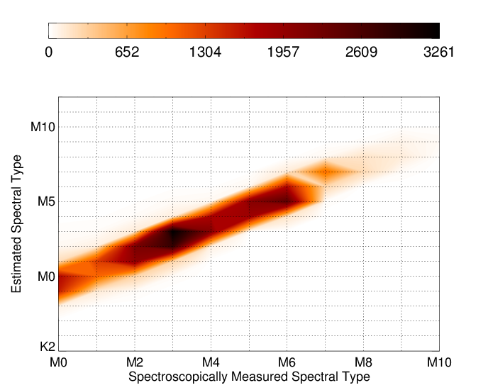
Figure 2: A 2-D histogram of the spectral types of known M dwarfs versus the spectral types found from the methods presented here, showing the accuracy of our spectral typing is $\sim\pm 1$. A colour version of this figure is available in the online article.

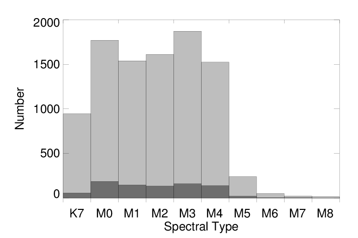
Figure 3: Histograms showing the frequency of each spectral type in the sample. The light grey is all stars with magnitude $J$$<$17, the dark grey $J$$<$15.

3.2 Variability Selection

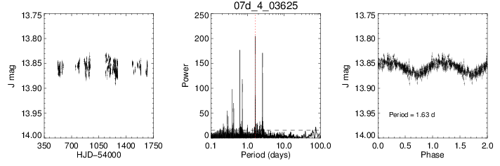
Figure 4: Example light curve and periodogram for variable star: From left to right: Observed $J$ band time series for star; Lomb-Scargle periodogram of time series between period window of 1 and 100 days with the maximum peak at 1.63 days. The dashed horizontal line represents the 99% confidence level, the red dashed line represents the peak corresponding to the period about which the lightcurve is to be folded; Phase folded light curve about period of 14.19 days with uncertainties omitted.

To identify periodically variable stars the frequency spectrum for each of the M dwarf light curves in the sample is found using the Lomb-Scargle periodogram, which is optimised for finding sinusoidal shaped periodic signals (Lomb, 1976; Scargle, 1982). The periodogram calculates a normalised power spectrum across a defined range of periods; the peaks corresponding to periodic variations in the light curve. It is robust with respect to a varying amplitude in that while a linear change in amplitude will attenuate a signal and a periodic change in amplitude will introduce a second signal, the signal corresponding to the primary variability period will still be detected. A false alarm probability (FAP, as described by Horne & Baliunas (1986)) threshold is determined to enable the peaks in the periodogram to be identified with a given level of confidence and to filter out peaks that are probably caused by noise. Our threshold is defined such that all peaks in the periodogram with a value greater than this value corresponds to a real signal with 99 per cent confidence or better, that is to say, we discard by default any peaks that are less probable than one generated by Gaussian noise by determining the power of such a peak. All other peaks are ignored and the remaining stars are retained as candidates for periodic variability. This process only eliminates peaks that are unlikely to be real signals, but leaves other signals that are not due to modulation by photospheric spots. These other sources of periodic variability are identified and eliminated from the sample. Potential sources that are discernible are identified as:

• Eclipsing binaries

• Other variable stars

• Periods imposed by the rotation of the Earth

• Periods imposed by sampling rates

• Periods from seeing variations with merged sources

One star was excluded as it was blended with the diffraction spike from a known Mira type star V1134 Cyg (Miller, 1966), evoking a period of 327.01 days. We discount all other potential identities for the variables for having too early a spectral type or too long a period as with RR Lyrae type stars or too large a light curve amplitude that would be indicative of semi-regular, Mira or other variable giant stars are excluded by the aforementioned colour cuts. A total of 12 suspected or know eclipsing binaries were identified in the sample as having light curves with periodic troughs of two distinct depths, indicative of the primary and secondary eclipse of the system, or periodic magnitude variations of $\Delta$$J$$>$0.02. We find amplitudes larger than this necessitate unphysical photospheric spot configurations using a light curve synthesis detailed in Section 5.3. These were excluded from the sample.

Light curves with periods corresponding to $\sim$1 day are identified, as is a sample of light curves with periods corresponding, within 3 significant figures, to fractions of a day (i.e. 1/2, 1/3, 1/4, 1/5), thought to be caused by repeated sampling at a 1 day period. These stars are not excluded from the search, but these periods are, such that these peaks in the periodogram are ignored while other peaks are identified. Additionally each variable star candidate is inspected by eye in the field to reduce the potential of having any variations in magnitude invoked by variability in other sources in a crowded field. For many light curves, the periodograms have multiple peaks above the FAP threshold, in which case the light curve is folded about the primary or highest peak. From the 68 light curves in the sample a peak to peak amplitude for each light curve is obtained by binning the folded lightcurve, while the period is obtained directly from the highest peak in the periodogram not to have been previously discounted, about which the light curve is folded.

Each light curve is then broken down in three separate consecutive epoch ranges each containing a third of the observations and each range is again tested for variability. While the significance of the peak in the periodogram varied for each epoch range, its presence ensures that the periodic signal is maintained in the photometry of the star for the duration of observations. This process also enables the discover of some examples of evolving variability as discussed in Section 5.2.

4 Results

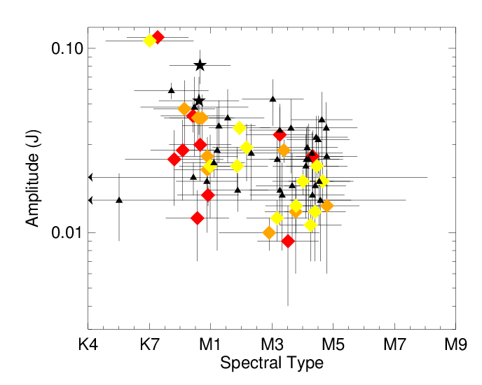
Figure 5: Estimated spectral type of each stars versus peak to peak J band amplitude in the folded light curves. The uncertainties in spectral type are the standard deviations of the spectral types found per colour index. Errors in amplitude are estimated from the errors in magnitude in the observed magnitudes. Symbols are described in the text. The Spearman rank correlation coefficient (R_S=-0.35) indicates a weak trend for decreasing amplitudes at later spectral types. A colour version of this figure is available in the online article.

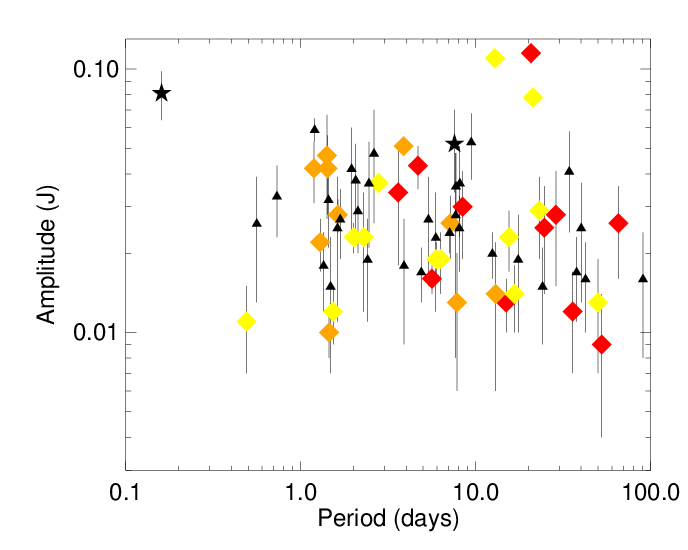
Figure 6: Variability period versus peak to peak amplitude. The periods correspond to those in Figures 15 onward, amplitude as in 5. Symbols are described in the text. The Spearman rank correlation coefficient (R_S=-0.24) indicates a weak trend for decreasing amplitudes at longer periods; it is less correlated than the trend found by Hartman et al. (2011). A colour version of this figure is available in the online article.

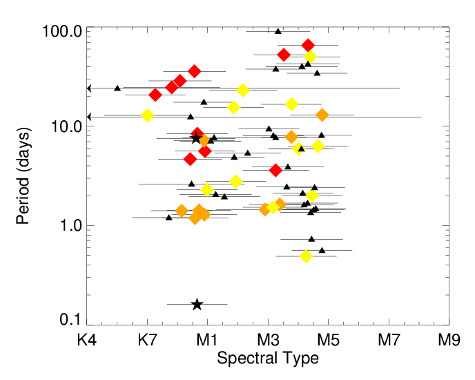
Figure 7: Estimated spectral type versus variability period. The periods correspond to those in Figures 15 onward, spectral type as in 5. Symbols are described in the text. A colour version of this figure is available in the online article.

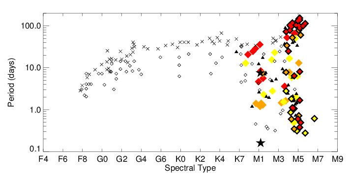
Figure 8: Estimated spectral type versus variability period, including objects from the later-type sample, and compilation of rotating field stars from the literature, presented in Irwin et al. (2011, Figure 12) for comparison. Symbols are described in the text, or else, the symbols with black borders being those from Irwin et al. (2011) with red, orange and yellow corresponding to their definitions of thick, middle and thin disc populations respectively; crosses represent young field stars ($\sim$1-2Gyr) and unfilled black diamonds represent old field stars ($\sim$8-10Gyr). Spectral types were interpolated from the standard spectral types and stellar masses (Mamajek, 2011). The large v_tan stars, which may be of the older, thick-disc population, with spectral type M1V ($\sim$0.6 $M_{\odot}$) are shown to exist with periods of $<$10 days, existing as outliers to the sequence of old rotators. A colour version of this figure is available in the online article.

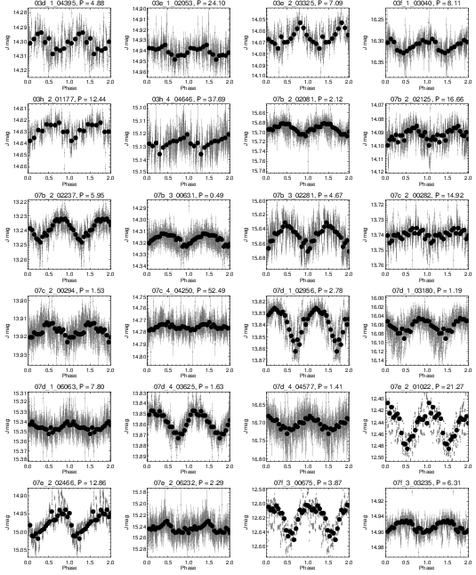
Figure 15: Folded light curves for the variable stars with estimated spectral times in the 03, 07 and 19 hour fields. Light curves are labeled with the name of the star and the period from from the periodogram.

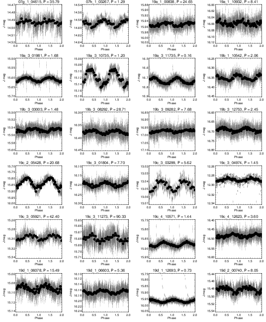
Figure 16: As in Figure 15.

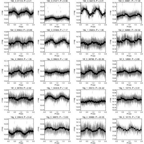
Figure 17: As in Figure 15.

The variability search yields 68 detections of variable stars (Table 2, Figures 15-17) with colours indicating they are late type dwarfs. A Spearman rank correlation coefficient calculated for the amplitudes with respect to spectral type finds a weak trend for lesser amplitudes at later spectral types (R_S=-0.35, 99.7% significance), with the largest amplitudes detected from the earliest type stars. Figure 6 shows amplitude against period, and while no upper envelope (e.g. Messina et al., 2003) is found, a weak trend for smaller amplitudes at longer periods is found using the same Spearman rank coefficient (R_S=-0.24, 95.5% significance), as Hartman et al. (2011) find in sample of periodically variable M dwarfs in the HATNet survey, although with a less defined and significant correlation. This would be expected to arise from the more rapid rotation of the short period variables driving an increase in magnetic activity, given the dependence of the $\alpha-\Omega$ dynamo on rotation. It should be noted that the random orientation of the axes of rotation of these stars would attenuate this correlation by mitigating the difference in flux observed along the line of site as an unevenly spotted star rotates. For stars with randomly distributed inclinations we would expect the peak amplitude to be on average $1/\sqrt{2}$ of the actual amplitude. The switch between radiative to fully convective occurs at types later than M3.5 (Rockenfeller et al., 2006), although this is not visible in Figures 5, 7, and 6 due to the lack of variable stars later than M4 detected in our sample.

We can take advantage of these results to make comparisons with rotation-evolution studies, using tangential velocities ($v_{t}$) obtained from SDSS proper motions and distance estimates from photometric parallaxes (Bochanski et al., 2011) as approximate tracers of population (eg. Reiners & Basri, 2008). We label stars with a $v_{t}\gtrsim 30$ kms^-1 as likely old disk stars (red diamonds in Figures 5, 6, 7, 8), and those with a $v_{t}<15$ as young disk stars (yellow diamonds). Other stars are marked with orange diamonds. Two of the faintest stars in our sample are found to have $v_{t}$=309$\pm$35 kms^-1 and $v_{t}$=814$\pm$79 kms^-1 (marked with black stars), consistent with being members of the halo. We find our old disk stars are primarily slower rotators, corroborating the results and collated data of Kiraga & Stȩpień (2007), and the later MV stars in Irwin et al. (2011), who find a greater number of slow rotators amongst the old disk stars, and also find young disk stars occupying the full range of detected periods. We find the majority our ’old’ stars at periods $>$20 days, in agreement with their conclusion of a more rapid spin down time for more massive, partially radiative stars. Although we do find 5 early MV stars with periods $<$10 days, this may be as a result of the crude method of assuming an age from $v_{tan}$ that does not take into account the full space velocity of the star, and these stars may in fact be members of the younger population, as early M types only remain active for $<$2Gyr (West et al., 2008).

5 Discussion

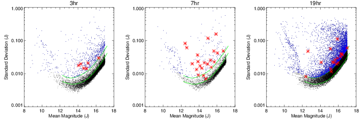
Figure 9: Dispersion (standard deviation) of each lightcurve versus magnitude. Red symbols indicate the mean brightness of the star versus the amplitudes in $J$ magnitude. The blue points are those that lay above the green line indicating the effective 1$\sigma$ and 2$\sigma$ boundaries. The majority stars with the larger standard deviation show detectable periodic variability but may be stochastically variable, while others are eclipsing binaries. A colour version of this figure is available in the online article.

5.1 Completeness

In our sample, the lack of detected variable late-MV stars may be reflective of the very low numbers of stars later then M4 (see Figure 3) present in the total sample, such that this lack of active stars beyond M7 may purely be indicative of the bias in the sample towards earlier spectral types, as we find no variables later than M4V. Ciardi et al. 2011 find a variability fraction of 0.367 for M dwarfs over the same observation window based on the dispersion of points in the lightcurves about the mean, but note that their sample includes stars that are not periodic in their variability. They also find that the time scales for such variability is on a time scales of weeks or more. Rockenfeller et al. (2006) find the fraction of variable stars among field M dwarfs to be $0.21\pm 0.11$. For periodically variable stars, we find a the variable fraction to be $\geq$0.007. For comparison, Hartman et al. (2011) find a fraction of 0.057 stars as reliable variables but 0.001 periodic and quasi-period variables amongst field M and K dwarfs in the HATNet survey.

standard deviation of each magnitude. Considering only the stars above the one an average fraction per magnitude bin (12$<$J$<$17)

In order to further assess the sensitivity of our period detection method, and to probe how noise in the light curves affects detections, we perform Monte Carlo simulations. These simulations are carried out in such a way to also determine the effects of aliasing of the observation periods with real periodic signals. Light curves with no intrinsic periodic signal are randomised with respect to magnitude, maintaining observation times. Sinusoidal signals of random periods and amplitudes are then injected. The same Lomb-Scargle periodogram is applied to each lightcurve and tested for a peak more significant than the 0.1 FAP threshold, corresponding to the injected period, which by our method would constitute a detection. The resulting simulations show that the for 12$<$$J$$<$15 periods of less than 20 days with a $J$ band variability greater than 0.01 should always be detected. Indeed this constitutes the majority of periodic variability detections despite a greater sample of stars at $J$$>$15. These simulations indicate that that for 12$<$$J$$<$14 the fraction of variable stars is is 2%. This variable fraction is still are an order of magnitude less than those found at surveys of shorter wavelengths, and reasons for this are discussed in section 5.3.

5.2 Variability

Periodicity only occurs for those M dwarfs that are active, and this activity also results in flaring. Reiners (2007) predicts that rotational periods of the order of several weeks will be found for early M dwarfs with difficulty, due to the relatively short duration flaring events resulting in noise disguising the periodicity. The WTS observations are however conducted in the $J$ band, which alleviates this issue as flaring events are rarely as detectable in the near infrared (Rockenfeller et al., 2006). Tofflemire et al. (2012) find no evidence of flaring in $JHK_{S}$ pass bands during simultaneous optical and infrared monitoring of three M dwarf stars for 47 hours corresponding to the flaring events they detect in the $U$-band. We have serendipitously found one particularly large flaring event from the M4V($\pm 1$) star 19d_1_12692, of $\geq$$\Delta 0.2$ in $J$ band magnitude. The incomplete observations of the flare lasted for 49 minutes and thus the overall duration could have been several hours. This brightness of the flare is in contrast to the results of Tofflemire et al. (2012) who expect to find flaring events in the $J$ band occurring on mmag scales, and would transform to a $u$-band response of $>$$\Delta 6$, which by extrapolation of the frequencies of flaring events per magnitude found by Davenport et al. (2012) would be expected to be observed less than once a year. Due to such a low rate of occurrence it is unlikely that such a flare would obfuscate a planetary transit, but such high intensity flares may have astrobiological significance.

Figure 10: The flare observed from the variable M4V star 19d_1_12693. Consecutive observations are joined. The observation of the flare is partial but those observations composing it were made over a 49 minute period.

In our sample we have detected M dwarfs with periods between hours and several weeks, with the largest period found at 50.02 days. For comparison, Messina et al. (2011) find 30 late-type periodic variable stars in the open cluster M11 with periods typically ranging between $\sim$1 day to $\sim$20 days, whilst Messina et al. (2003) finds dwarf stars with spectral types K4-M6 with periods between $\sim$1 and $\sim$10 days. Irwin et al. (2011) similarly find long periods, in a wavelength region approximately corresponding to the $i+z$ bands for M dwarfs ranging between 0.28 and 154 days in their study of rotating M dwarfs in the MEarth Transit Survey. Benedict et al. (1998) find evidence for periodicity in Barnard’s Star of $\sim$130 days and Proxima Centauri of $\sim$40 and $\sim$83 days, the latter confirmed by Kiraga & Stȩpień (2007). Whilst the WTS periodic variable M dwarf sample produced no convincing evidence of periodicity on these time scales, a large number of periods $>$ 80 days were found in the periodicity search and subsequently rejected when no sinusoidal variability was seen. Indeed it is not expected that all spot coverage on a star will induce a periodic variability in brightness if the spot coverage is not sufficiently inhomogeneous to invoke a detectable difference in brightness as the star rotates, or if the spot coverage changes in morphology at shorter time scales than the rotation period, although even in such a case a rotation period should be found by a Lomb-Scargle periodogram. This is discussed further in the following section.

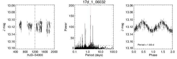
Figure 11: As in Figure 15. For 17d_1_06032, periodic variability was only found from the latter 50% of the observations, as marked, while no significant peak corresponding to this period was found when the periodogram was performed over all observations. Indeed a change in the amplitude of the unfolded lightcurve is visible across the marked division. This could be due to evolution in the spots on the photosphere such that, during the course of the observations, the spot coverage became less uniform so as to become variably bright.

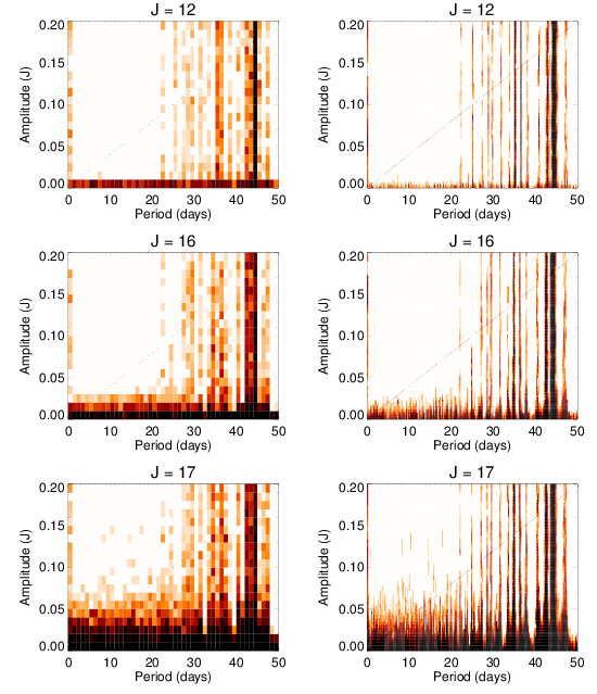
Figure 13: Fractions of injected signal detected for lightcurve amplitude as a function of period. White presents a retrieval fraction of 1 (i.e. a signal corresponding to the period with a probability $>$.99 of a real signal not caused by noise is retrieved in every simulation) and black a fraction of 0 (i.e. no significant signal corresponding to the injected period is found and noise dominates in all simulations). The plots on the left show the output binned at 1 day period intervals and 0.01 $J$ band magnitude amplitude intervals with an average of 1666.7 data per bin, and on the right at 0.25 day and 0.005 $J$ band magnitude intervals respectively with an average of 4.2 data per bin. A window of high-retrievability remains for the brightest targets for $J$ = 12 to $J$ = 15 with detectability decreasing at $J$ $>$ 16. The diagrams on the right show a very strong dependency on period due to aliasing effects with periods of observation. Please see online article for a colour version of this figure.

From our simulations discussed in Section 5.1 and shown in Figure 13 there is substantial loss of completeness for periods $>$20 days due to aliasing effects. In observations with Kepler Ciardi et al. (2011) find that M dwarfs are primarily variable over these time scales or longer. We are therefore limited to detecting only a smaller subsection of M dwarfs before our detection rate becomes sensitive to aliasing with observational periods, despite the overall long base line of observation time.

5.3 Spot Morphology

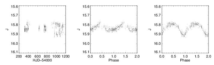
Figure 12: The upper plots show light curves with errors omitted of the stars 19c_2_05428 and folded about the same period of 20.68 days, with the centre panel showing observations at HJD$<$54900 and the panel on the left with observations at HJD$>$54900. The low plots show and 07e_2_02466 and folded about the same period of 12.86 days, with the centre panel showing observations at HJD$<$55000 and the panel on the left with observations at HJD$>$55000. For 19c_2_05428, the phase is conserved, although the two distinct amplitudes and morphologies show the dichotomous nature of the variability over time. This may be an indicator of longitude dependent spots or spot groups evolving over time. 07e_2_02466 however exhibits a similar saw tooth like morphology in both sets of observations but the amplitude appears to vary more stochastically, although over hundreds of days.

We find some evidence for a change in spot coverage was found in one star with an indeterminate spectral type in the 17hr field, 17d_1_06032 (Figure 11), and in the stars 07e_2_02466 and 19c_2_05428 (Figure 12). In the former, no significant peak in the periodogram, performed over the entire series of observations, corresponded to an obvious periodicity in folded light curves, thought the most significant peak in the periodogram for only the later 50% of the observations did correspond to a period for which a folded light curve displayed obvious periodic behavior. In the latter two a strong peak corresponding to the period is found in their periodograms although the amplitude of the variation changes over timescale of months, perhaps similarly indicative in a change in the spottedness of the stars. The changes in both instances happened over a time scale of $<$100 days, although due to a lack of observations during the transition it is unknown what the true speed of the amplitude change was. In both 17d_1_06032 and 19c_2_05428 however, the change in amplitude was dichotomous and does not appear to vary much once the new amplitude if established, whereas in 07e_2_02466 the amplitude varies over hundreds of days.

Since little information is known about the distribution of spots on any of the M dwarfs in our sample, a spot model is used to generate a range of scenarios against which the results presented here can be compared. The simulations were generated by the Doppler Tomography of Stars code (DoTS) (Collier Cameron, 1997) that can produce synthetic light curves at a chosen wavelength (13000Å, corresponding approximately to the $J$ band midpoint) for a range of photospheric and spot temperatures ($T_{p}$, $T_{s}$ respectively) and spot coverage models. The spot coverage models are identical to those used by Barnes et al. (2011), including seven models in total covering solar minimal and maximum coverage to more extreme cases for active stars (see Table 1, Barnes et al., 2011). Three $T_{p}/T_{s}$ ratios are used for each coverage model, a solar like ratio of 0.6, a less extreme ratio of 0.8, and an adjustment such that $T_{s}=T_{p}-250$ K, comparable to models fitted to variable field M dwarfs in $G$, $R$, $I$ bands by (Rockenfeller et al., 2006). In addition to these models a single spot model at the 0.6 contrast ratio and -250K contrast were simulated for comparison with randomly distributed spot models. In these models a single 5$\degree$ wide spot was places at 0$\degree$ latitude on a star of zero inclination. Each simulation is carried out for a range of effective temperatures corresponding from spectral types M0V to M10V at 250K intervals, based on mass-spectral class models by Baraffe & Chabrier (1996) and a spectral type-effective temperature scale derived by Mohanty & Basri (2003).

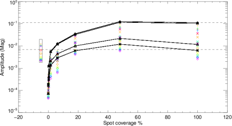
Figure 14: Output from the DoTS code of peak to peak amplitudes for simulated light curves against the spot coverage percentage. Coloured diamonds, crosses and pluses indicate $J$ band scenarios for $T_{s}=T_{p}-250$K, $T_{s}=0.8T_{p}$ and $T_{s}=0.6T_{p}$ with each colour representing a photosphere temperate from 2250K (red) to 3750K (magenta) in 250K steps. The joined stars indicate the analogous maximum and minimum $I$ band amplitudes in each case, and the triangle the analogous $V$ band amplitudes respectively. The dashed lines represent the range of amplitudes detected in our sample of variable stars; the low limit imposed by the noise limitation in WTS. The boxed points show the amplitudes found by having one large spot group located on the stars equator. The $I$ and $V$ band amplitudes for the less spotted cases are larger, indicating that we are sampling stars with activities greater then $\sim 10$ per cent and that surveys in the $J$ band such as WTS may not be sensitive to lower amplitude variability in the less spotted cases than surveys at shorter wavelengths. The amplitude downturn between the two most heavily spotted models is due to the increase in homogeneity as the the spot coverages tends towards totality, such that the temperature differentials on the photosphere become dominated by the lesser contrast between spot umbrae and penumbrae rather than the greater contrast between spotted and unspotted areas. Please see online article for a colour version of this figure.

From the simulations, synthetic light curves are obtained giving a range of peak to peak amplitudes for each scenario of spot coverage, against which the variable stars in the sample can be compared in order to place limits on the spot coverage of each star. The results of the DoTS simulations are plotted in Figure 14. These simulations place some limits on the spot coverage over the variable M dwarfs found here that suggest a star spot coverage modeled at 18% and 48% for lower $T_{s}/T_{p}$ ratios and a lower coverage model at 6.1% for the larger $T_{s}/T_{p}=0.6$ model. Also included in this range are many of the single spot models, although the morphology of these is distinct from a sinusoid and we can rule out such models as an explanation for the variability we detect. There exists numerous degeneracies between models and scenarios not modeled here rendering further determinations of spot coverage difficult. The single spot model included a spot of 5$\degree$ width centered at 0$\degree$ latitude, although larger spots at changing latitudes could generate the same peak to peak amplitude, and there maybe be multiple spots or spotted regions. The light curves for these configurations would differ in shape, as modeled by Frasca et al. (2009), but such shape is difficult to distinguish due to noise in the WTS light curves, in addition with the potential for individual spots to change in size over the duration of the survey. Furthermore, the amplitudes are highly dependent on the $T_{s}/T_{p}$ ratio which introduces extra degeneracy. While a well defined spot coverage cannot be determined, it is apparent that many of the lightcurves are not sinusoids, instead resembling a saw tooth morphology (Figures 15, 16, 17), suggesting a spot density that is more sharply dependent on longitude.

The detection of stars with amplitudes $\Delta$J$>0.1$ is at least evidence for spot coverage $\gtrsim$50$\%$, as required to explain observations of M dwarf radii by Jackson et al. (2009), assuming a more random distribution of spot coverage, or large variation in the spottedness of such a star with respect to longitude.Additionally, some information can be extracted from comparisons between the $V$, $I$ and $J$ band amplitudes. The amplitudes in the $V$ and $I$ bands are greater for stars with lower spot coverages which may explain discrepancies between the variable fraction found here and the higher fractions found in the aforementioned surveys. Simulations show that $J$ band amplitudes for any given spot induced variability are 0.44 of those in the $V$ band and 0.55 of those in the $I$ band. Furthermore, the simulations indicate we are limited to detecting only stars with spot coverages greater than $\sim$10 per cent, as variability possible under lesser spotted models is of a lesser amplitude then the noise limit of WTS, and affirms the use of the near infra-red for planetary transit searches as spot induced variability is of a lesser magnitude that that observed in shorter wavelengths. Indeed, in variable samples observed at shorter wavelengths such as Rockenfeller et al. (2006) ($R$, $I$) and Irwin et al. (2011) ($\sim$$i+z$ bands) find lightcurve amplitudes of the order of $\sim$0.005-0.01 in their respective pass bands. In the sample described in Rockenfeller et al. (2006) only 16% of the detected $I$ band amplitudes are $>$0.02 in magnitude. Lower level variability scaled to the $J$ band would be less than the range detectable in our sample due to our noise limitations found in our Monte Carlo simulations, which reflect the general noise limit of the WTS (Figure 9). This, coupled with aliasing sensitivity for periods $>$20 days, may explain the order of magnitude lower fraction of periodically variable M dwarfs detected in our $J$ band survey.

6 Conclusions

In this paper we have selected a sample of M dwarfs from the WFCAM Transit Survey by estimating their spectral type using colour indexes. From this a sub-sample of variable objects are selected using a Lomb-Scargle periodogram. 68 variable rotating MV stars are found with a range of periods from 0.16 to 90.03 days and amplitudes from 0.009 to 0.115 in the $J$ band. Additionally three others with a less constrained spectral type are found. We infer population membership from tangential velocities and find our results to be in agreement with previous such studies.

Using a lightcurve synthesis code we find that these stars may have a high degree of spottedness, of the order of 10 per cent surface coverage or more, in some cases $\gtrsim$50 per cent, at least at time scales of $<20$ days, and we estimated a fraction for these variable M dwarfs of at least of 1 per cent from the most complete subsamples. These results indicate that transit surveys carried out in the $J$ band may be less susceptible to the effect of spot induced variability in photometric observations, as our simulations suggest they are predisposed to only detecting the variability of the most active of M dwarfs. This would minimise intrinsic variability and allow the better parameterisation of transiting planet and eclipsing binary systems by observing in the near infrared. One example of a particular large flare in the $J$ band is serendipitously found. We also find evidence for evolving spot morphologies in the form of light curve amplitudes varying over periods of months in three of stars. In one late type dwarf of unknown spectral type periodic variability was found to switch on after months of inactivity.

7 Acknowledgments

GB and BS are supported by Rocky Planets Around Cool Stars (RoPACS), a Marie Curie Initial Training Network funded by the European Commission’s Seventh Framework Programme.

NG, JB, DP, SH, JB, HJ, CdB, M-CG-O, SN and EM have received support from RoPACS during this research, a Marie Curie Initial Training Network funded by the European Commission’s Seventh Framework Programme.

This work was partly funded by the by the Fundação para a Ciência e a Tecnologia (FCT)-Portugal through the project PEst-OE/EEI/UI0066/2011

We would like to thank collaborators across the RoPACS network for their useful comments. We acknowledge a useful contribution from Peter Hensmen towards this project.

Appendix A

Name	RAa	Deca	Jb	ST Est.c	Pd	ae	PM${}_{\alpha}^{f}$	PM${}_{\delta}^{f}$	v${}_{t}^{g}$
03d_1_04395	55.115972	39.134701	14.32	M1 $\pm$ 1.01	4.880	0.017 $\pm$ 0.004	—	—	—
03e_1_02053	53.784274	38.954377	14.95	K5 $\pm$ 9.36	24.100	0.015 $\pm$ 0.006	—	—	—
03e_2_03325	54.204782	38.846530	14.08	M1 $\pm$ 1.01	7.090	0.024 $\pm$ 0.004	—	—	—
03f_1_03040	54.006089	38.807408	16.30	M4 $\pm$ 1.01	8.110	0.037 $\pm$ 0.014	—	—	—
03h_2_01177	55.772275	38.959886	14.64	K9 $\pm$ 7.64	12.440	0.020 $\pm$ 0.004	—	—	—
03h_4_04646	55.184813	39.423991	15.13	M3 $\pm$ 1.00	37.690	0.017 $\pm$ 0.006	—	—	—
07b_2_02081	106.059460	12.868579	15.69	M4 $\pm$ 1.00	2.120	0.029 $\pm$ 0.009	—	—	—
07b_2_02125	106.158970	12.867247	14.10	M3 $\pm$ 1.00	16.660	0.014 $\pm$ 0.004	-1.410 $\pm$ 2.642	-1.606 $\pm$ 2.642	3.047 $\pm$ 0.624
07b_2_02237	106.272010	12.863213	13.24	M4 $\pm$ 1.00	5.950	0.019 $\pm$ 0.003	-16.955 $\pm$ 2.547	6.120 $\pm$ 2.547	15.996 $\pm$ 1.925
07b_3_00631	106.072930	13.345031	14.31	M4 $\pm$ 1.01	0.490	0.011 $\pm$ 0.004	-1.657 $\pm$ 2.853	-1.733 $\pm$ 2.853	3.317 $\pm$ 0.705
07b_3_02281	106.137370	13.257735	15.64	K9 $\pm$ 1.06	4.670	0.043 $\pm$ 0.008	-4.709 $\pm$ 2.797	-3.696 $\pm$ 2.797	49.275 $\pm$ 9.840
07c_2_00282	106.827750	12.938019	13.71	G9 $\pm$ 2.70	14.920	0.013 $\pm$ 0.003	0.142 $\pm$ 2.421	-3.279 $\pm$ 2.421	115.837 $\pm$ 22.843
07c_2_00294	106.899370	12.937313	13.91	M3 $\pm$ 1.00	1.530	0.012 $\pm$ 0.003	9.569 $\pm$ 2.617	-2.292 $\pm$ 2.617	16.275 $\pm$ 2.652
07c_4_04250	106.459880	13.336219	14.76	M3 $\pm$ 1.00	52.490	0.009 $\pm$ 0.005	1.724 $\pm$ 2.924	-19.953 $\pm$ 2.924	42.274 $\pm$ 9.217
07d_1_02956	106.627350	12.859053	13.83	M1 $\pm$ 1.00	2.780	0.037 $\pm$ 0.003	-3.240 $\pm$ 2.481	-1.363 $\pm$ 2.481	7.927 $\pm$ 1.486
07d_1_03180	106.617910	12.780124	16.04	M0 $\pm$ 1.11	1.190	0.042 $\pm$ 0.011	-3.872 $\pm$ 2.970	-0.899 $\pm$ 2.970	37.971 $\pm$ 8.498
07d_1_06063	106.510690	12.913766	15.35	M3 $\pm$ 1.00	7.800	0.013 $\pm$ 0.007	8.695 $\pm$ 3.114	-1.453 $\pm$ 3.114	22.054 $\pm$ 4.435
07d_4_03625	106.725960	13.303723	13.87	M3 $\pm$ 1.00	1.630	0.028 $\pm$ 0.004	5.903 $\pm$ 2.561	-16.933 $\pm$ 2.561	27.624 $\pm$ 4.870
07d_4_04577	106.692980	13.339136	16.70	K9 $\pm$ 1.01	1.410	0.047 $\pm$ 0.020	-1.171 $\pm$ 3.130	1.261 $\pm$ 3.130	25.460 $\pm$ 6.040
07e_2_01022	105.870700	12.686058	12.45	K2 $\pm$ 2.20	21.270	0.078 $\pm$ 0.002	-3.729 $\pm$ 2.322	1.183 $\pm$ 2.322	12.746 $\pm$ 2.243
07e_2_02466	105.869530	12.632173	14.99	K7 $\pm$ 1.44	12.860	0.110 $\pm$ 0.007	-1.946 $\pm$ 2.392	-0.524 $\pm$ 2.392	16.488 $\pm$ 3.097
07e_2_06232	105.994080	12.512096	15.27	M0 $\pm$ 1.01	2.290	0.023 $\pm$ 0.011	0.327 $\pm$ 2.764	-0.321 $\pm$ 2.764	2.618 $\pm$ 0.580
07f_3_00675	106.076750	13.042346	12.62	G5 $\pm$ 20.00	3.870	0.051 $\pm$ 0.002	-11.750 $\pm$ 2.322	-1.021 $\pm$ 2.322	34.156 $\pm$ 4.526
07f_3_03235	106.172640	13.106071	14.94	M4 $\pm$ 1.00	6.310	0.019 $\pm$ 0.005	-4.006 $\pm$ 3.053	-6.566 $\pm$ 3.053	13.356 $\pm$ 2.988
07g_1_04615	106.386640	12.613818	14.49	M0 $\pm$ 1.03	35.790	0.012 $\pm$ 0.005	-14.678 $\pm$ 2.514	-8.399 $\pm$ 2.514	77.421 $\pm$ 10.105
07h_1_03267	106.617800	12.550436	14.59	M0 $\pm$ 1.08	1.290	0.022 $\pm$ 0.005	0.743 $\pm$ 2.616	-5.523 $\pm$ 2.616	22.316 $\pm$ 4.654
19a_1_00838	292.765130	36.419518	15.99	K8 $\pm$ 1.61	24.650	0.025 $\pm$ 0.011	1.516 $\pm$ 2.956	-3.306 $\pm$ 2.956	39.212 $\pm$ 3.310
19a_1_10932	292.511620	36.308370	16.08	M0 $\pm$ 1.02	8.410	0.030 $\pm$ 0.011	5.269 $\pm$ 4.318	2.332 $\pm$ 4.318	52.077 $\pm$ 6.235
19a_3_01981	293.095110	36.809146	15.64	M4 $\pm$ 1.00	1.680	0.027 $\pm$ 0.008	—	—	—
19a_3_10735	293.304660	36.915622	15.14	K8 $\pm$ 1.21	1.200	0.059 $\pm$ 0.006	—	—	—
19a_3_11735	293.329960	36.744529	16.78	M0 $\pm$ 1.00	0.160	0.081 $\pm$ 0.017	-36.959 $\pm$ 4.379	51.498 $\pm$ 4.379	813.932 $\pm$ 78.904
19b_1_10542	292.815320	36.294256	16.36	M1 $\pm$ 1.19	2.060	0.038 $\pm$ 0.014	—	—	—
19b_3_03003	293.389460	36.815246	15.58	M4 $\pm$ 1.00	1.480	0.015 $\pm$ 0.008	—	—	—
19b_3_08292	293.505170	36.904554	16.39	K9 $\pm$ 1.05	28.710	0.028 $\pm$ 0.013	1.228 $\pm$ 3.669	-3.199 $\pm$ 3.669	44.699 $\pm$ 4.699
19b_3_09282	293.527870	36.925772	16.99	M1 $\pm$ 1.06	7.680	0.028 $\pm$ 0.020	—	—	—
19b_3_12753	293.601230	36.745270	16.71	M3 $\pm$ 1.01	2.450	0.037 $\pm$ 0.016	—	—	—
19c_2_05428	294.422680	36.416670	15.91	K7 $\pm$ 1.00	20.680	0.115 $\pm$ 0.010	2.969 $\pm$ 2.681	-2.105 $\pm$ 2.681	41.374 $\pm$ 3.151
19c_3_01804	294.179440	36.758408	16.27	M3 $\pm$ 1.00	7.700	0.036 $\pm$ 0.012	—	—	—
19c_3_03299	294.205130	36.760331	13.17	M0 $\pm$ 1.00	5.620	0.016 $\pm$ 0.002	7.245 $\pm$ 2.438	-18.289 $\pm$ 2.438	42.647 $\pm$ 2.796
19c_3_04974	294.235120	36.750789	12.41	M2 $\pm$ 1.64	1.450	0.010 $\pm$ 0.002	-10.040 $\pm$ 2.393	0.388 $\pm$ 2.393	21.279 $\pm$ 1.379
19c_3_05921	294.252830	36.875064	15.37	M4 $\pm$ 1.05	42.400	0.016 $\pm$ 0.006	—	—	—
19c_3_11273	294.354460	36.709272	15.75	M3 $\pm$ 1.06	90.330	0.016 $\pm$ 0.008	—	—	—
19c_4_10571	293.851810	36.888130	15.92	M4 $\pm$ 1.02	1.440	0.032 $\pm$ 0.011	—	—	—
19c_4_12623	293.864930	36.921243	16.54	M3 $\pm$ 1.10	3.600	0.034 $\pm$ 0.016	3.934 $\pm$ 5.675	-17.812 $\pm$ 5.675	88.260 $\pm$ 14.006
19d_1_06078	294.046830	36.381880	15.14	M1 $\pm$ 1.00	15.490	0.023 $\pm$ 0.006	2.722 $\pm$ 3.513	2.695 $\pm$ 3.513	15.304 $\pm$ 1.497
19d_1_06603	294.036450	36.297312	16.21	M2 $\pm$ 1.10	5.360	0.027 $\pm$ 0.012	—	—	—
19d_1_12693	293.923010	36.287590	16.00	M4 $\pm$ 1.03	0.730	0.033 $\pm$ 0.010	—	—	—
19d_2_00740	294.453090	36.487943	15.54	M3 $\pm$ 1.00	8.050	0.025 $\pm$ 0.008	—	—	—
19d_3_01140	294.441370	36.901497	15.64	M4 $\pm$ 1.01	2.410	0.019 $\pm$ 0.008	—	—	—
19d_3_01271	294.445960	36.921308	16.38	M4 $\pm$ 1.00	0.560	0.026 $\pm$ 0.013	—	—	—
19d_3_01937	294.455060	36.830460	12.63	M3 $\pm$ 1.00	0.470	0.045 $\pm$ 0.002	-17.728 $\pm$ 2.344	1.854 $\pm$ 2.344	23.887 $\pm$ 1.434
19d_3_02216	294.461610	36.796780	14.10	M4 $\pm$ 1.00	2.010	0.023 $\pm$ 0.003	12.883 $\pm$ 4.176	5.053 $\pm$ 4.176	14.979 $\pm$ 1.616
19d_3_03681	294.482160	36.713086	15.83	M0 $\pm$ 1.00	17.480	0.019 $\pm$ 0.009	—	—	—
19d_3_05922	294.526470	36.803361	16.08	M2 $\pm$ 1.12	23.060	0.029 $\pm$ 0.010	-0.337 $\pm$ 3.841	2.172 $\pm$ 3.841	11.717 $\pm$ 1.263
19d_3_07286	294.550410	36.755946	15.38	M0 $\pm$ 1.00	7.170	0.026 $\pm$ 0.007	1.442 $\pm$ 2.741	4.024 $\pm$ 2.741	25.633 $\pm$ 1.961
19e_1_03204	292.733110	36.090610	16.79	M1 $\pm$ 1.19	1.950	0.042 $\pm$ 0.018	—	—	—
19e_2_02880	293.130710	36.239925	15.18	M4 $\pm$ 1.00	50.020	0.013 $\pm$ 0.006	3.037 $\pm$ 3.696	3.874 $\pm$ 3.696	8.848 $\pm$ 0.920
19e_2_09200	293.301440	36.154486	15.22	M4 $\pm$ 1.00	1.350	0.018 $\pm$ 0.006	—	—	—
19e_3_09622	293.199860	36.614838	16.46	M4 $\pm$ 1.00	1.620	0.025 $\pm$ 0.014	—	—	—
19f_3_08798	293.508310	36.571411	15.98	M4 $\pm$ 1.00	65.390	0.026 $\pm$ 0.010	12.862 $\pm$ 4.506	13.205 $\pm$ 4.506	39.388 $\pm$ 4.858
19f_3_12800	293.593410	36.489227	15.97	M3 $\pm$ 1.18	3.890	0.018 $\pm$ 0.009	—	—	—
19f_4_06780	292.808650	36.620585	17.02	M0 $\pm$ 1.76	2.620	0.048 $\pm$ 0.022	—	—	—
19g_1_04348	293.805310	36.117012	16.34	M0 $\pm$ 1.06	1.420	0.042 $\pm$ 0.014	3.106 $\pm$ 3.109	1.070 $\pm$ 3.109	32.632 $\pm$ 2.962
19g_1_05313	293.787750	36.249911	16.76	M4 $\pm$ 1.00	34.220	0.041 $\pm$ 0.017	—	—	—
19g_1_10773	293.683380	36.080351	16.16	M4 $\pm$ 1.08	5.910	0.023 $\pm$ 0.011	—	—	—
19g_2_03649	294.179550	36.224328	16.47	M3 $\pm$ 1.00	9.420	0.053 $\pm$ 0.015	—	—	—
19g_3_06870	294.268510	36.556675	15.62	M4 $\pm$ 1.06	13.000	0.014 $\pm$ 0.008	-8.732 $\pm$ 3.748	-1.280 $\pm$ 3.748	18.177 $\pm$ 1.921
19g_4_00989	293.744820	36.504677	16.20	M4 $\pm$ 1.20	40.050	0.025 $\pm$ 0.012	—	—	—
19h_3_16170	294.703050	36.655522	16.99	M0 $\pm$ 1.31	7.560	0.052 $\pm$ 0.018	-5.934 $\pm$ 3.846	-12.512 $\pm$ 3.846	309.087 $\pm$ 34.741

a Coordinates in SDSS (epoch J2000) if available

b WTS average UKIDSS system $J$ band magnitude MKO system

c Spectral type estimate as determined by method described in Section 3.1 with error determined by standard deviation in colour-type space and minimum uncertainty of $\pm$1 (see Figure 2)

d Period in days as determined by maximum peak in Lomb-Scargle periodogram

e Amplitude in $J$ band magnitude

f Proper motion in masyr-1 from SDSS

g Tangential velocity in kms-1

Table 2: A table of the 68 variable M dwarfs found. Included are stars outside the M dwarf spectral type range but with H-K $>$ 0.175 suggesting a redder, late type star that the spectral typing procedure erroneous assigned an earlier spectral type, and have been retained for maximum inclusivity. Spectroscopic follow up is required to absolutely confirm the nature of these stars, and any subsequent exclusion would not effect the conclusions we draw.

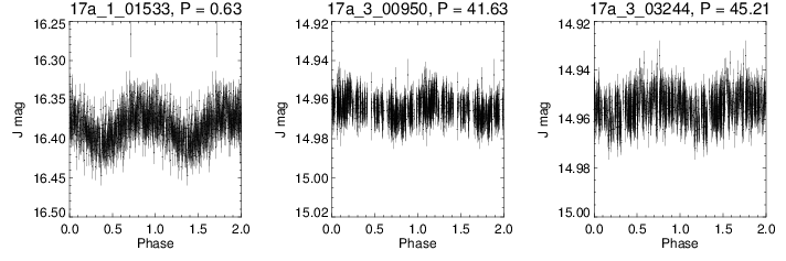
Figure 18: As in Figure 4. These light curves are the periodically variable stars found in the 17hr field for which there are no observations in the SDSS and therefore no spectral type estimation were made.

References

- Baraffe & Chabrier (1996) Baraffe, I. & Chabrier, G. 1996, ApJL, 461, L51+
- Barnes et al. (2002) Barnes, J., James, D., & Cameron, A. 2002, Astronomische Nachrichten, 323, 333
- Barnes et al. (2011) Barnes, J. R., Jeffers, S. V., & Jones, H. R. A. 2011, MNRAS, 412, 1599
- Benedict et al. (1998) Benedict, G. F., McArthur, B., Nelan, E., et al. 1998, AJ, 116, 429
- Berta et al. (2012) Berta, Z. K., Irwin, J., Charbonneau, D., Burke, C. J., & Falco, E. E. 2012, ArXiv e-prints
- Bochanski et al. (2011) Bochanski, J. J., Hawley, S. L., & West, A. A. 2011, AJ, 141, 98
- Borucki et al. (2011) Borucki, W. J., Koch, D. G., Basri, G., et al. 2011, ApJ, 736, 19
- Brown et al. (2008) Brown, B. P., Browning, M. K., Brun, A. S., Miesch, M. S., & Toomre, J. 2008, ApJ, 689, 1354
- Browning et al. (2010) Browning, M. K., Basri, G., Marcy, G. W., West, A. A., & Zhang, J. 2010, AJ, 139, 504
- Chabrier & Küker (2006) Chabrier, G. & Küker, M. 2006, A&A, 446, 1027
- Charbonneau et al. (2009) Charbonneau, D., Berta, Z. K., Irwin, J., et al. 2009, Nature, 462, 891
- Ciardi et al. (2011) Ciardi, D. R., von Braun, K., Bryden, G., et al. 2011, AJ, 141, 108
- Collier Cameron (1997) Collier Cameron, A. 1997, MNRAS, 287, 556
- Coughlin et al. (2008) Coughlin, J. L., Stringfellow, G. S., Becker, A. C., et al. 2008, ApJL, 689, L149
- Covey et al. (2007) Covey, K. R. et al. 2007, Astron. J., 134, 2398
- Davenport et al. (2012) Davenport, J. R. A., Becker, A. C., Kowalski, A. F., et al. 2012, ApJ, 748, 58
- Frasca et al. (2009) Frasca, A., Covino, E., Spezzi, L., et al. 2009, A&A, 508, 1313
- Fressin et al. (2011) Fressin, F., Torres, G., Rowe, J. F., et al. 2011, ArXiv e-prints
- Gillon et al. (2007) Gillon, M., Pont, F., Demory, B.-O., et al. 2007, A&A, 472, L13
- Granzer et al. (2000) Granzer, T., Schüssler, M., Caligari, P., & Strassmeier, K. G. 2000, A&A, 355, 1087
- Hartman et al. (2011) Hartman, J. D., Bakos, G. Á., Noyes, R. W., et al. 2011, AJ, 141, 166
- Hewett et al. (2006) Hewett, P. C., Warren, S. J., Leggett, S. K., & Hodgkin, S. T. 2006, Mon. Not. Roy. Astron. Soc., 367, 454
- Horne & Baliunas (1986) Horne, J. H. & Baliunas, S. L. 1986, ApJ, 302, 757
- Irwin et al. (2011) Irwin, J., Berta, Z. K., Burke, C. J., et al. 2011, ApJ, 727, 56
- Irwin et al. (2007) Irwin, J., Irwin, M., Aigrain, S., et al. 2007, MNRAS, 375, 1449
- Jackson et al. (2009) Jackson, R. J., Jeffries, R. D., & Maxted, P. F. L. 2009, MNRAS, 399, L89
- Jeffers et al. (2007) Jeffers, S. V., Donati, J.-F., & Collier Cameron, A. 2007, MNRAS, 375, 567
- Johnson et al. (2012) Johnson, J. A., Gazak, J. Z., Apps, K., et al. 2012, AJ, 143, 111
- Kiraga & Stȩpień (2007) Kiraga, M. & Stȩpień, K. 2007, Acta Astron., 57, 149
- Kovács, G. and Hodgkin, S. and Sipőcz, B and Pinfield, D., and others (2012) Kovács, G. and Hodgkin, S. and Sipőcz, B and Pinfield, D., and others. 2012, in prep
- Lomb (1976) Lomb, N. R. 1976, APSS, 39, 447
- Mamajek (2011) Mamajek, E. 2011, A Modern Mean Stellar Color and Effective Temperatures (Teff) Sequence for O9V-Y0V Dwarf Stars, See http://www.pas.rochester.edu/emamajek/EEM_dwarf _UBVIJHK_colors_Teff.dat [Online; accessed 09-August-2012]
- Messina et al. (2011) Messina, S., Desidera, S., Lanzafame, A. C., Turatto, M., & Guinan, E. F. 2011, A&A, 532, A10+
- Messina et al. (2003) Messina, S., Pizzolato, N., Guinan, E. F., & Rodonò, M. 2003, A&A, 410, 671
- Miller et al. (2008) Miller, A. A., Irwin, J., Aigrain, S., Hodgkin, S., & Hebb, L. 2008, MNRAS, 387, 349
- Miller (1966) Miller, W. J. 1966, Ricerche Astronomiche, 7, 217
- Mohanty & Basri (2003) Mohanty, S. & Basri, G. 2003, ApJ, 583, 451
- Morales et al. (2010) Morales, J. C., Gallardo, J., Ribas, I., et al. 2010, ApJ, 718, 502
- Moreno-Insertis et al. (1992) Moreno-Insertis, F., Schüssler, M., & Ferriz-Mas, A. 1992, A&A, 264, 686
- Morin et al. (2008) Morin, J., Donati, J.-F., Petit, P., et al. 2008, MNRAS, 390, 567
- Morin et al. (2010) Morin, J., Donati, J.-F., Petit, P., et al. 2010, MNRAS, 407, 2269
- Muirhead et al. (2012) Muirhead, P. S., Johnson, J. A., Apps, K., et al. 2012, ArXiv e-prints
- Nefs et al. (2012) Nefs, S. V., Birkby, J. L., Snellen, I. A. G., et al. 2012, ArXiv e-prints
- Plavchan et al. (2008) Plavchan, P., Jura, M., Kirkpatrick, J. D., Cutri, R. M., & Gallagher, S. C. 2008, ApJS, 175, 191
- Reiners (2007) Reiners, A. 2007, A&A, 467, 259
- Reiners & Basri (2008) Reiners, A. & Basri, G. 2008, ApJ, 684, 1390
- Rockenfeller et al. (2006) Rockenfeller, B., Bailer-Jones, C. A. L., & Mundt, R. 2006, A&A, 448, 1111
- Scargle (1982) Scargle, J. D. 1982, ApJ, 263, 835
- Schuessler & Solanki (1992) Schuessler, M. & Solanki, S. K. 1992, A&A, 264, L13
- Tofflemire et al. (2012) Tofflemire, B. M., Wisniewski, J. P., Kowalski, A. F., et al. 2012, AJ, 143, 12
- Vogt et al. (2010) Vogt, S. S., Butler, R. P., Rivera, E. J., et al. 2010, ApJ, 723, 954
- West et al. (2008) West, A. A., Hawley, S. L., Bochanski, J. J., et al. 2008, AJ, 135, 785
- West et al. (2011) West, A. A., Morgan, D. P., Bochanski, J. J., et al. 2011, AJ, 141, 97