Spin-polarized conductance in double quantum dots:
Interplay of Kondo, Zeeman and interference effects

Abstract

We study the effect of a magnetic field in the Kondo regime of a double-quantum-dot system consisting of a strongly correlated dot (the “side dot”) coupled to a second, noninteracting dot that also connects two external leads. We show, using the numerical renormalization group, that application of an in-plane magnetic field sets up a subtle interplay between electronic interference, Kondo physics, and Zeeman splitting with nontrivial consequences for spectral and transport properties. The value of the side-dot spectral function at the Fermi level exhibits a nonuniversal field dependence that can be understood using a form of the Friedel sum rule that appropriately accounts for the presence of an energy- and spin-dependent hybridization function. The applied field also accentuates the exchange-mediated interdot coupling, which dominates the ground state at intermediate fields leading to the formation of antiparallel magnetic moments on the dots. By tuning gate voltages and the magnetic field, one can achieve complete spin polarization of the linear conductance between the leads, raising the prospect of applications of the device as a highly tunable spin filter. The system’s low-energy properties are qualitatively unchanged by the presence of weak on-site Coulomb repulsion within the second dot.

I Introduction

Electron correlations in quantum-dot structures result in many fascinating effects that can be probed in detail with remarkable experimental control of system parameters.Gordon1 ; Marcus ; Cronenwett Perhaps one of the most interesting regimes occurs when electrons confined in the dot acquire antiferromagnetic correlations with electrons in the leads, giving rise to the well-known Kondo effect.Hewson The simplest realization of this phenomenon in a single quantum dot is characterized by just one low-energy scale, set by the Kondo temperature, which controls (among other features) the width of a many-body resonance at the Fermi energy.Gordon1 ; Hewson Recent experimentalDQD1 ; DQD2 ; DQD3 ; DQD4 ; DQD5 ; vdWiel studies of the Kondo effect in multiple quantum dots have revealed a complex competition between geometry and correlations, making evident that these structures provide a flexible setting in which to explore much novel physics.

In this context, double-quantum-dot arrangements exhibit striking manifestations of Kondo physics, with conductance signatures of these effects predicted to show up in realistic experimental setups. A telling example is the interplay of Kondo physics and quantum interference in “side-coupled” or “hanging-dot” configurations, Apel_EPJB04 ; Busser ; Cornaglia ; Tanaka_PRB2005 ; Zitko1 ; Tanaka2008 ; ZitkoFano ; Tanaka2012 ; Irisnei2011 leading to a variety of interesting “Fano-Kondo” effects. SpinPolRMP A rather unexpected situation arises when a small, strongly interacting “dot 1” is connected to external leads via a large “dot 2” that is tuned to have a single-particle level in resonance with the common Fermi energy of the leads.Dias1 ; DiasComment ; Dias2 In this configuration the Kondo resonance, which normally has a single peak at the Fermi energy, splits into two peaks—a behavior that can be understood as a consequence of interference between the many-body Kondo state in dot 1 and a single-particle-like resonance that controls (or “filters”) its connection to the leads.Dias1 ; DiasComment ; Dias2 ; Aligia The magnitude of the Kondo peak splitting is determined by the balance of several important energy scales in the problem: the width and position of the active single-particle level in dot 2; the height of the effective single-particle resonance set by the interdot coupling; and the many-body Kondo temperature (determined by the preceding energy scales in combination with the dot-1 level-position and interaction strength). This filtering of the leads preserves a fully screened Kondo ground state with a Kondo temperature that rises with increasing interdot coupling.

In this work, we investigate the effects of an external in-plane magnetic field on such a double-quantum dot-system in the side-dot arrangement. The field—which introduces another energy scale, the Zeeman energy—is known to be detrimental to the Kondo state in single-dot systems.Andrei ; Gordon1 ; Hofstetter ; Costi00 ; Logan:JPCM:9713:2001 Using numerical renormalization-group methods,NRG ; Hofstetter we study the interplay between the different energy scales and discuss the behavior of the Kondo resonance in the presence of competing interactions. This interplay reveals itself in the fundamental Fermi-liquid properties of the system, such as the variation with magnetic field $B$ at zero temperature of the Fermi-energy ($\omega=0$) value of the side-dot spectral function $A_{1}(\omega,T)$. Instead of the usual monotonic decayCosti00 ; Logan:JPCM:9713:2001 of $A_{1}(0,0)$ with increasing $B$ we find a markedly nonuniversal behavior, where $A_{1}(0,0)$ passes through a maximum at a nonzero value of the field. This effective field-enhancement of the Kondo spectral function is a consequence of the side-dot geometry. The same behavior can also be understood using an appropriate form of the Friedel sum rule, which predicts parameter- and field-dependent phase shifts that impart the unusual nonmonotonicity to the variation of $A_{1}(0,0)$ with $B$.

In addition, we show that the competition between Zeeman splitting of the dot levels and Kondo screening results in a dominant exchange-mediated antiferromagnetic coupling of the dots over a range of moderate magnetic fields, before both dots become fully polarized at higher fields. Finally, we identify signatures of the aforementioned phenomena in the transport properties. A key result is the generation of spin-polarized currents through the device, which can be tuned by adjusting gate voltages to achieve total polarization.

The remainder of the paper is organized as follows: In Sec. II we describe the effective Anderson impurity model for the double-quantum-dot system. Section III presents the low-energy spectral properties, while Sec. IV interprets the nonuniversal behavior of $A_{1}(\omega=0,T=0)$ vs $B$ in terms of the Friedel sum rule. The transport properties, including spin polarization, are explored in Sec. V. Concluding remarks appear in Sec. VI.

II Double-quantum-dot system

The system under study, which is depicted schematically in Fig. 1, contains two quantum dots. Dot 1 has a large Coulomb repulsion $U_{1}$ when its single active energy level is doubly occupied. Dot 2 has negligible electron-electron interactions ($U_{2}\simeq 0$) and one active level that can be tuned by gate voltages to be at or near resonance with the common Fermi energy $\epsilon_{F}=0$ of left ($L$) and right ($R$) leads. Electrons can tunnel between dots 1 and 2 with tunneling matrix element $\lambda$, and between dot 2 and lead $\ell$ with tunneling matrix element $V_{2\ell}$.

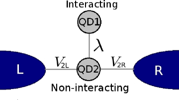
Figure 1: (Color online) Schematic representation of the side-coupled double-quantum-dot system. The dot QD1 has a strong Coulomb interaction $U_{1}$ and is coupled only to the second dot, labeled QD2. The latter dot has negligible local interactions (i.e., $U_{2}\simeq 0$) and the energy of its active level is tuned to allow tunneling at or near resonance with the Fermi level of the left ($L$) and right ($R$) leads.

The system can be described by a variant of the two-impurity Anderson Hamiltonian:

$$H=H_{\mathrm{dots}}+H_{\mathrm{leads}}+H_{\mathrm{hyb}},$$ (1)

with

$$H_{\mathrm{dots}} =\sum_{i=1,2}\Biggl{(}\sum_{\sigma}\varepsilon_{i\sigma}n_{i\sigma}+U_{i}n_{i\uparrow}n_{i\downarrow}\Biggr{)}$$

$$\qquad+\lambda\sum_{\sigma}\bigl{(}d_{1\sigma}^{{\dagger}}d_{2\sigma}^{\phantom{\dagger}}+\mathrm{H.c.}\bigr{)},$$ (2)

$$H_{\mathrm{leads}} =\sum_{\ell=L,R}\sum_{\mathbf{k},\sigma}\varepsilon_{\ell\mathbf{k}\sigma}c_{\ell\mathbf{k}\sigma}^{{\dagger}}c_{\ell\mathbf{k}\sigma}^{\phantom{\dagger}}\,,$$ (3)

and

$$H_{\mathrm{hyb}}=\sum_{\ell=L,R}V_{2\ell}\sum_{\mathbf{k},\sigma}\bigl{(}d_{2\sigma}^{{\dagger}}c_{\ell\mathbf{k}\sigma}^{\phantom{\dagger}}+\mathrm{H.c.}\bigr{)}.$$ (4)

Here, $d_{i\sigma}$ annihilates an electron in dot $i$ with spin $z$ component ${\textstyle\frac{1}{2}}\sigma$ ($\sigma=\pm 1$ or equivalently $\uparrow,\>\downarrow$) and energy $\varepsilon_{i\sigma}=\varepsilon_{i}+{\textstyle\frac{1}{2}}\sigma g_{i}\mu_{B}B$ ; $n_{i\sigma}=d_{i\sigma}^{{\dagger}}d_{i\sigma}^{\phantom{\dagger}}$ is the corresponding number operator; and $c_{\ell\mathbf{k}\sigma}$ annihilates an electron in lead $\ell$ with spin $z$ component ${\textstyle\frac{1}{2}}\sigma$ and energy $\varepsilon_{\ell\mathbf{k}\sigma}=\varepsilon_{\ell\mathbf{k}}+{\textstyle\frac{1}{2}}\sigma g_{c}\mu_{B}B$. The magnetic field $B\hat{\mathbf{z}}$ with $B\geq 0$ is assumed to lie in the plane of the two-dimensional electron gas in which the dots and leads are defined, so that it produces no kinematic effects and enters only through Zeeman level splittings. This Hamiltonian differs from a generic two-impurity Anderson model through the absence of dot-1 hybridizations $V_{1\ell}$, a consequence of the side-dot geometry. Throughout the greater part of the paper, we also take $U_{2}=0$, a case that is particularly convenient for algebraic analysis. The effect of nonvanishing dot-2 interactions is addressed at the end of Sec. V.

Without loss of generality, we take all tunneling matrix elements to be real. We consider local ($\mathbf{k}$-independent) dot-lead tunneling and assume that the dots have equal effective $g$ factors $g_{1}=g_{2}=g$, simplifications that do not qualitatively affect the physics. The leads are taken to have featureless band structures near the Fermi energy, modeled by the flat-top densities of states $\rho_{L}(\omega)=\rho_{R}(\omega)=\rho(\omega)=(2D)^{-1}\Theta(D-|\omega|)$ where $D$ is the half-bandwidth and $\Theta(x)$ is the Heaviside function. The equilibrium and linear-response properties of the system may be calculatedone-eff-band by considering the coupling of dot 2 via hybridization matrix element $V_{2}=\sqrt{V_{2L}^{2}+V_{2R}^{2}}$ to a single effective conduction band described by annihilation operators $c_{\mathbf{k}\sigma}=(V_{2L}c_{L\mathbf{k}\sigma}+V_{2R}c_{R\mathbf{k}\sigma})/V_{2}$ and a density of states $\rho(\omega)$. The Zeeman splitting of this conduction band produces only very small effects near the band edges, so for convenience we set the bulk $g$ factor to $g_{c}=0$ throughout what follows.

The primary quantities of interest in this work are the retarded dot Green’s functions ${\cal G}_{i\sigma}(\omega,T)=\langle\langle d_{i\sigma}^{\phantom{\dagger}};d_{i\sigma}^{{\dagger}}\rangle\rangle_{\omega}$ for $i=1,\,2$, where $\langle\langle A;B\rangle\rangle_{\omega}=-i\int_{0}^{\infty}\langle\{A(t),B(0)\}\rangle e^{i\omega t}dt$ and $\langle\cdots\rangle$ denotes an appropriate thermal average.Zubarev In particular, we are interested in the spectral functions $A_{i\sigma}(\omega,T)=-\pi^{-1}\mathrm{Im}\,\mathcal{G}_{i\sigma}(\omega,T)$ and the system’s linear (zero-bias) conductance, given by the Meir-Wingreen formulaMeir_Wingreen as $G=\sum_{\sigma}G_{\sigma}$ with

$$G_{\sigma}(T)={\textstyle\frac{1}{2}}\,G_{0}\int_{-\infty}^{\infty}[-\mathrm{Im}\,\mathcal{T}_{\sigma}(\omega,T)]\,(-\partial f/\partial\omega)\,d\omega,$$ (5)

where $f(\omega,T)$ is the Fermi distribution function at temperature $T$ and $G_{0}=[2V_{2L}V_{2R}/(V_{2L}^{2}+V_{2R}^{2})]^{2}(2e^{2}/h)$ represents the unitary conductance of a single channel of electrons multiplied by a factorone-eff-band ; LoganPRB2009 that varies between 1 (for $V_{2L}=V_{2R}$) and 0 (in the limit of extreme left-right asymmetry of the dot-tunneling). In the side-connected geometry, the transmission isApel_EPJB04 ; Cornaglia ; Dias2

$$\mathcal{T}_{\sigma}(\omega,T)=\Delta_{2}\,\mathcal{G}_{2\sigma}(\omega,T),$$ (6)

where $\Delta_{2}=\pi V^{2}_{2}/2D$. Thus,

$$2G_{\sigma}(T)/G_{0}=\pi\Delta_{2}\int_{-\infty}^{\infty}A_{2\sigma}(\omega,T)\,(-\partial f/\partial\omega)\,d\omega,$$ (7)

which reduces at zero temperature to

$$2G_{\sigma}(T=0)/G_{0}=\pi\Delta_{2}A_{2\sigma}(0,0).$$ (8)

In order calculate the dot spectral functions $A_{i\sigma}(\omega,T)$ taking full account of the electronic correlations arising from the $U_{1}$ term in Eq. (II), we employ the numerical renormalization-group (NRG) method, performing a logarithmic discretization of the conduction band and iteratively solving the discretized Hamiltonian. In evaluating the spectral functions, we perform a Gaussian-logarithmic broadening of discrete poles obtained by the procedure described in Ref. Bulla01, . At temperatures $T>0$ we use the density-matrix variant of the NRG,Hofstetter which has better spectral resolution at high frequencies and nonzero fields.Hofstetter ; NRG Although these schemes are not totally free from systematic errors, BroadeningMagField the main results of the paper do not depend crucially on the broadening procedure.

All numerical results were obtained for a symmetric dot 1 described by $U_{1}=-2\varepsilon_{1}$, for dot 2 width $\Delta_{2}=0.02$, and for NRG discretization parameter $\Lambda=2.5$. Except where it is stated otherwise, we consider a strongly correlated dot 1 with $U_{1}=0.5$ and situations in which a noninteracting dot 2 is tuned to be in resonance with the leads, i.e., $U_{2}=\varepsilon_{2}=0$. We adopt units in which $D=\hbar=k_{B}=g\mu_{B}=1$.

III Spectral Properties

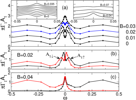
Figure 2: (Color online) (a) Spin-averaged dot-1 spectral function $A_{1}$ vs frequency $\omega$ at zero temperature for $U_{1}=-2\varepsilon_{1}=0.5$, $\varepsilon_{2}=0$, $\lambda=0.0627$, and (from bottom to top curve, offset for clarity) $B=0$, $0.01$, $0.02$, and $0.03$. The spectral function is multiplied by $\pi\Gamma_{1}$ where $\Gamma_{1}=\lambda^{2}/\Delta_{2}$. Insets: Expanded views of $A_{1}$ vs $\omega$ around the Fermi level $\omega=0$ for the same system, with $B$ ranging from $0$ to $0.035$ (bottom to top, curves offset for clarity) in steps of $0.005$ in the left inset, and from $0.04$ to $0.07$ (bottom to top, curves offset for clarity) in steps of $0.01$ in the right inset. (b) Spin-up (black squares) and spin-down (red circles) dot-1 spectral functions $A_{1\sigma}(\omega,T=0)$ for $B=0.02$ with all other parameters as in (a). (c) Same as (b), except for $B=0.04$.

In single quantum dots, the presence of an in-plane magnetic field Hofstetter or connection to ferromagnetic leadsMartinek modifies coherent spin fluctuations and weakens the Kondo effect. The spin-averaged spectral function exhibits a Kondo-peak splitting that grows with increasing applied field, while the value of the spectral function at the Fermi energy decreases monotonically. In this section we investigate the effects of a Zeeman field on the side-dot spectral function in the double-dot system defined in Sec. II.

Figure 2(a) shows the spin-averaged spectral function

$$A_{1}(\omega,T)={\textstyle\frac{1}{2}}[A_{1\uparrow}(\omega,T)+A_{1\downarrow}(\omega,T)]$$ (9)

for a side-dot setup at zero temperature with $U_{1}=0.5$ and $\lambda=0.0627$. The different curves, vertically offset for clarity, correspond to four different values of $B$. For zero field (the bottom curve), $A_{1\uparrow}(\omega,0)=A_{1\downarrow}(\omega,0)=A_{1}(\omega,0)$, so each spin-resolved spectral function shows a symmetric Kondo-peak splitting due to the interdot coupling $\lambda$. With increasing $B$, the split peaks merge into a single peak at $\omega=0$, clearly seen for $B=0.03$ (top curve). The left inset to Fig. 2(a) shows in greater detail the convergence of the peaks near the Fermi energy, with the maximum in $A_{1}$ vs $\omega$ at $\omega=0$ being best defined at $B=0.035$, a field where, incidentally, the absolute value of $A_{1}(0,0)$ exceeds that at $B=0$ by nearly a factor of two. For slightly larger fields, the central peak again splits into two before all low-energy features become flattened out at fields $B\geq 0.07$ [right inset to Fig. 2(a)].

The field-induced merging of the peaks in $A_{1}(\omega,0)$ arises from opposite displacements of $A_{1\uparrow}(\omega,0)$ and $A_{1\downarrow}(\omega,0)$ along the $\omega$ axis. In a nonzero magnetic field, $A_{1\sigma}(\omega,T)\neq A_{1\sigma}(-\omega,T)$ but $A_{1\uparrow}(\omega,T)=A_{1\downarrow}(-\omega,T)$. This is illustrated for $B=0.02$ in Fig. 2(b), which also shows that the heights of the two peaks in each spin-resolved spectral function $A_{1\sigma}(\omega,0)$ are no longer equal. Upon further increase in the field to $B=0.04$ [Fig. 2(c)], the double-peak structure is replaced by a single peak near $\omega=0$ in each spin-resolved spectral function. For larger values of $B$, these peaks move away from the Fermi energy and the usual Zeeman-splitting of the Kondo peak with decreasing amplitude becomes evident in the spin-averaged spectral function [right inset in Fig. 2(a)]. This behavior can be qualitatively understood by considering the evolution with $B$ of the level energies foundVaugier2007 in the “atomic limit” $\Delta_{2}=0$ where the dots are isolated from the leads.

We now focus on the field dependence of $A_{1}(\omega=0,T=0)$, a quantity that acts as a sensitive measure of the interplay of the different energy scales in the problem: the single-particle resonance width $\Delta_{2}$, the zero-field Kondo temperature $T_{K}$, and the Zeeman energy $g\mu_{B}B$. Figure 3(a) plots $\pi\Delta(0)\,A_{1}(0,0)$ vs $B/T_{K}$ (taking $g\mu_{B}=1$) for six values of $\lambda$. The energy scale $\Delta(0)$, introduced for normalization purposes, is defined in Eq. (26) below. For now, it suffices to note that $\Delta(0)$ is proportional to $[1+(B/2\Delta_{2})^{2}]^{-1}$, i.e., it is a decreasing function of the field. The figure reveals two distinct regimes of behavior: (1) For $\lambda\lesssim 0.05$, $\pi\Delta(0)\,A_{1}(0,0)$ decreases monotonically from its zero-field value $1$ over a characteristic field scale that increases with $\lambda$ (and is not simply $T_{K}$, as it is in the single-dot case). (2) For $\lambda>0.05$, $\pi\Delta(0)\,A_{1}(0,0)$ has a nonmonotonic variation with increasing $B$, reaching a second maximum $\pi\Delta(0)\,A_{1}(0,0)=1$ at $B=B^{*}\simeq 2T_{K}$, beyond which field it decreases. In view of the field dependence of $\Delta(0)$, the value of $A_{1}(0,0)$ at $B=B^{*}$ is $[1+(B^{*}/2\Delta_{2})^{2}]$ times its zero-field counterpart. The two regimes seen in Fig. 3(a) are in sharp contrast with the monotonically decreasing and universal dependence of the Fermi-energy spectral function on $B/T_{K}$ in the conventional single-impurity KondoCosti00 and AndersonLogan:JPCM:9713:2001 models. The next section discusses these behaviors in terms of the Friedel sum rule.

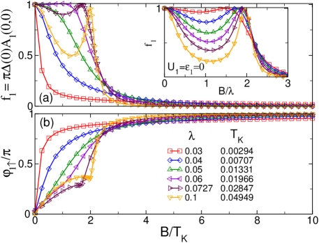
Figure 3: (Color online) (a) Spin-averaged dot-1 spectral function at the Fermi level $A_{1}(\omega\!=\!0,\,T\!=\!0)$ vs scaled magnetic field $B/T_{K}$ for $U_{1}=-2\varepsilon_{1}=0.5$, $\varepsilon_{2}=0$, and six values of $\lambda$. $A_{1}(0,0)$ has been multiplied by the field-dependent quantity $\pi\Delta(0)$ [Eq. (26)] to yield $f_{1}(B)$ defined in Eq. (25). The larger $\lambda$ values produce a nonmonotonic field variation of $A_{1}(0,0)$, with a peak around $B\simeq 2T_{K}$. Inset: Corresponding plot for the noninteracting case $U_{1}=\varepsilon_{1}=0$, with the field scaled by the interdot coupling $\lambda$. (b) Phase factor $\varphi_{1\uparrow}=-\varphi_{1\downarrow}$ corresponding to the data in (a), determined from the Friedel sum rule [Eq. (27)] using the magnetization data plotted in Fig. 4.

IV Friedel Sum Rule

In Sec. IV.1 we review the Fermi-liquid relation known as the Friedel sum ruleLangreth1966 ; Hewson that sets the Fermi-energy value of the zero-temperature spectral function in the one-impurity Anderson model, and write down a form of the sum rule valid for systems featuring both a Zeeman field and nontrivial structure in the density of states. Section IV.2 shows how the variation of $A_{1}(\omega=0,T=0)$ in our double-quantum-dot system can also be understood in terms of the Friedel sum rule.

IV.1 Single Anderson impurity

We consider a single-impurity Anderson model

$$H =\sum_{\sigma}\varepsilon_{d\sigma}n_{d\sigma}+Un_{d\uparrow}n_{d\downarrow}+\sum_{\mathbf{k},\sigma}\varepsilon_{\mathbf{k}\sigma}c_{\mathbf{k}\sigma}^{{\dagger}}c_{\mathbf{k}\sigma}^{\phantom{\dagger}}$$

$$\qquad+\sum_{\mathbf{k},\sigma}\bigl{(}V_{\mathbf{k}}d_{\sigma}^{{\dagger}}c_{\mathbf{k}\sigma}^{\phantom{\dagger}}+\mathrm{H.c.}\bigr{)},$$ (10)

where $\varepsilon_{d\sigma}=\varepsilon_{d}+{\textstyle\frac{1}{2}}\sigma g\mu_{B}B$ and $\varepsilon_{\mathbf{k}\sigma}=\varepsilon_{\mathbf{k}}+{\textstyle\frac{1}{2}}\sigma g_{c}\mu_{B}B$. The conduction-band dispersion $\varepsilon_{\mathbf{k}}$ and the hybridization $V_{\mathbf{k}}$ enter the impurity properties only in a single combination: the zero-field hybridization function $\Delta_{0}(\omega)=\pi\sum_{\mathbf{k}}|V_{\mathbf{k}}|^{2}\delta(\omega-\varepsilon_{\mathbf{k}})$. We denote the fully interacting retarded impurity Green’s for this problem by

$$\mathcal{G}_{d\sigma}(\omega,T)=\langle\langle d_{\sigma}^{\phantom{\dagger}};d_{\sigma}^{{\dagger}}\rangle\rangle_{\omega}=\frac{1}{\omega+i0^{+}-\varepsilon_{d\sigma}-\Sigma_{d\sigma}(\omega,T)}\,,$$ (11)

where $\Sigma_{d\sigma}(\omega,T)$ is the retarded impurity self-energy.

In the conventional Anderson model, where the hybridization function is assumed to take a flat-top form $\Delta_{0}(\omega)=\Gamma\Theta(D-|\omega|)$, the Friedel sum rule relates the Fermi-energy value of the zero-temperature, zero-field impurity spectral function $A_{d}(\omega,0)\equiv A_{d\sigma}(\omega,0)=-\pi^{-1}\mathrm{Im}\,\mathcal{G}_{d\sigma}(\omega,0)$ to the average impurity occupancy $\langle n_{d}\rangle=\langle n_{d\uparrow}\rangle+\langle n_{d\downarrow}\rangle$ as

$$\pi\Gamma A_{d}(0,0)=\sin^{2}\left(\frac{\pi}{2}\langle n_{d}\rangle\right)\,.$$ (12)

In the wide-band limit where $D$ greatly exceeds all other energy scales in the problem, Eq. (12) has been extended WrightPRB2011 to show that in a Zeeman field $B$, the spin-averaged impurity spectral function $A_{d}(\omega,T)={\textstyle\frac{1}{2}}[A_{d\uparrow}(\omega,T)+A_{d\downarrow}(\omega,T)]$ satisfies

$$\pi\Gamma A_{d}(0,0)={\textstyle\frac{1}{2}}\bigl{[}1-\cos(\pi\langle n_{d}\rangle)\,\cos\bigl{(}2\pi M_{d})\bigr{]},$$ (13)

where $M_{d}(B)={\textstyle\frac{1}{2}}(\langle n_{d\uparrow}\rangle-\langle n_{d\downarrow}\rangle)$ is the impurity magnetization in units of $g\mu_{B}$.

Our goal is to extend Eqs. (12) and (13) to allow for finite values of $D$ and any form of $\Delta_{0}(\omega)$. One can showHewson ; DiasComment ; Vaugier2007 ; Aligia ; LoganPRB2009 that provided the system is in a Fermi-liquid regime [where the imaginary part of $\Sigma_{d\sigma}(\omega,T=0)$ varies as $\omega^{2}$ for $\omega\to 0$], the spin-resolved spectral functions at zero temperature satisfy

$$\pi\Delta_{\sigma}(0)\,A_{d\sigma}(0,0)=\sin^{2}\bigl{(}\pi\langle n_{d\sigma}\rangle+\varphi_{\sigma}\bigr{)},$$ (14)

where $\Delta_{\sigma}(\omega)=\Delta_{0}(\omega-{\textstyle\frac{1}{2}}\sigma g_{c}\mu_{B}B)$ and

$$\varphi_{\sigma}=\mathrm{Im}\int_{-\infty}^{0}\frac{\partial\Sigma_{d\sigma}^{0}(\omega,T=0)}{\partial\omega}\,\mathcal{G}_{d\sigma}(\omega,T=0)\;d\omega$$ (15)

is a spin-dependent phase shift. In Eq. (15), $\mathcal{G}_{d\sigma}(\omega,T)$ is the fully interacting retarded impurity Green’s function specified in Eq. (11), but $\Sigma_{d\sigma}^{0}(\omega,T)$ is the retarded impurity self-energy for the noninteracting system [Eq. (IV.1) with $U=0$], which satisfies $\mathrm{Im}\,\Sigma_{d\sigma}^{0}(\omega,T)=-\Delta_{\sigma}(\omega)$.

In situations where $\Delta_{\uparrow}(\omega)\neq\Delta_{\downarrow}(\omega)$, it is convenient to focus on a dimensionless, hybridization-weighted average of the spin-resolved spectral functions:

$$F(\omega,T)=\frac{\pi}{2}\sum_{\sigma}\Delta_{\sigma}(\omega)A_{d\sigma}(\omega,T).$$ (16)

In terms of this quantity, the linear conductance is

$$G(T)=G_{0}\int_{-\infty}^{\infty}F(\omega,T)\,(-\partial f/\partial\omega)\,d\omega$$ (17)

with a zero-temperature limit

$$G(T=0)=G_{0}\,F(0,0).$$ (18)

Here, $G_{0}=[2V_{L}V_{R}/(V_{L}^{2}+V_{R}^{2})]^{2}(2e^{2}/h)$ is the maximum possible conductance through the dot for hybridizations $V_{L}$ and $V_{R}$ with the left and right leads, respectively. We note that the hybridization-weighted, spin-averaged spectral function reduces to $F(\omega,T)=\pi\Delta(\omega)\,A_{d}(\omega,T)$ for (i) all values of $\omega$ in zero magnetic field, and (ii) at $\omega=0$ for any field $B$ such that $\Delta_{0}\bigl{(}{\textstyle\frac{1}{2}}g_{c}\mu_{B}B\bigr{)}=\Delta_{0}\bigl{(}-{\textstyle\frac{1}{2}}g_{c}\mu_{B}B\bigr{)}$.

Inserting Eq. (14) into Eq. (16), rewriting $\langle n_{d\sigma}\rangle={\textstyle\frac{1}{2}}\langle n_{d}\rangle+\sigma M_{d}$, and defining $\varphi_{\pm}=\varphi_{\uparrow}\pm\varphi_{\downarrow}$, one obtains

$$F(0,0)={\textstyle\frac{1}{2}}\bigl{[}1-\cos(\pi\langle n_{d}\rangle+\varphi_{+})\,\cos\bigl{(}2\pi M_{d}+\varphi_{-})\bigr{]}.$$ (19)

This form of the Friedel sum rule relates the value of the hybridization-weighted spin-averaged spectral function at $\omega=0$ and $T=0$ to the impurity occupancy, the impurity magnetization, and spin-dependent phase factors that account for the energy dependence of the hybridization function. The right-hand side of Eq. (19) has a maximum possible value of 1, implying through Eq. (18) that $G(T=0)\leq G_{0}$, as one would expect for a problem with a single transmission mode in the left and right leads.

In general, each of the phase factors $\varphi_{\uparrow}$ and $\varphi_{\downarrow}$ has a complicated dependence on $\Delta(\omega)$, the impurity parameters $U$ and $\varepsilon_{d}$, and the magnetic field $B$. This makes it highly improbable that for a generic choice of model parameters there exists a value of $B$ for which the system satisfies the requirements

$$\cos(\pi\langle n_{d}\rangle+\varphi_{+})=-\cos\bigl{(}2\pi M_{d}+\varphi_{-})=\pm 1$$ (20)

for achieving $F(0,0)=1$ and, hence, a maximum conductance $G(T=0)=G_{0}$.

However, under conditions where both the impurity and the conduction band exhibit particle-hole symmetry, the Hamiltonian (1) is invariant under the transformation $d_{\sigma}^{\phantom{\dagger}}\to-d_{-\sigma}^{{\dagger}}$, $c_{\mathbf{k}\sigma}^{\phantom{\dagger}}\to c_{\mathbf{k},-\sigma}^{{\dagger}}$, $\varepsilon_{\mathbf{k}}\to-\varepsilon_{\mathbf{k}}$. This invariance leads to the relations $\Delta_{\uparrow}(\omega)=\Delta_{\downarrow}(-\omega)$, $\Sigma_{d\uparrow}^{0}(\omega,T)=-[\Sigma_{d\downarrow}^{0}(-\omega,T)]^{*}$ and $\mathcal{G}_{d\uparrow}(\omega,T)=-[\mathcal{G}_{d\downarrow}(-\omega,T)]^{*}$, which in turn imply that $A_{d\uparrow}(\omega,T)=A_{d\downarrow}(-\omega,T)$ and $\varphi_{\uparrow}=-\varphi_{\downarrow}$ (or $\varphi_{+}=0$). Since particle-hole symmetry also ensures $\Delta_{0}(\omega)=\Delta_{0}(-\omega)$ and $\langle n_{d}\rangle=1$, it follows that $\Delta_{\uparrow}(0)=\Delta_{\downarrow}(0)$ and the Friedel sum rule reduces to

$$\pi\Delta(0)\,A_{d}(0,0)=\cos^{2}\bigl{(}\pi M_{d}+\varphi_{\uparrow}).$$ (21)

In situations described by Eq. (21), the conductance will reach its maximum possible value $G_{0}$ whenever $(\pi M_{d}+\varphi_{\uparrow})/\pi$ equals an integer. It is much more likely that this single condition can be met at some value of $B$ than that a system away from particle-hole symmetry can be tuned to satisfy both parts of Eq. (20).

The conventional flat-top hybridization function $\Delta_{0}(\omega)=\Gamma\Theta(D-|\omega|)$ is not only particle-hole symmetric, but yields vanishingly small values of $\varphi_{\sigma}$, thereby simplifying Eq. (19) to the previously derivedWrightPRB2011 Eq. (13). One expects $|M_{d}(B)|$ to be an increasing function of $B$ with a limiting value $|M_{d}(B\to\infty)|={\textstyle\frac{1}{2}}$, and therefore [via Eq. (13)] both $A_{d}(0,0)$ and $G(T=0)$ should decrease monotonically with increasing $B$.

IV.2 Double quantum dots

We now return to the double-quantum-dot setup defined in Eq. (1). It has been shownDias1 that for the special case $U_{2}=0$, the properties of dot 1 are identical to those of the impurity in a single-impurity Anderson model [Eq. (IV.1)] with $U=U_{1}$, $\varepsilon_{d}=\varepsilon_{1}$, and a zero-field hybridization function

$$\Delta_{0}(\omega)=\pi\lambda^{2}\rho_{2}(\omega),$$ (22)

where

$$\rho_{2}(\omega)=\frac{1}{\pi}\frac{\Delta_{2}}{(\omega-\varepsilon_{2})^{2}+\Delta_{2}^{2}}$$ (23)

describes a unit-normalized Lorentzian resonance of width $\Delta_{2}$ [defined after Eq. (6)] centered on energy $\omega=\varepsilon_{2}$.

In a Zeeman field $B$, where the spin-dependent hybridization function of the effective one-impurity problem is

$$\Delta_{\sigma}(\omega)=\Delta_{0}\bigl{(}\omega-{\textstyle\frac{1}{2}}\sigma g\mu_{B}B\bigr{)},$$ (24)

a quantity of interest is

$$f_{1}(B)=\frac{\pi}{2}\sum_{\sigma}\Delta_{\sigma}(0)\,A_{1\sigma}(0,0),$$ (25)

the value of the hybridization-weighted spin-averaged dot-1 spectral function at $\omega=T=0$. For the resonant case $\varepsilon_{2}=0$ considered in Figs. 2 and 3,

$$\Delta_{\uparrow}(0)=\Delta_{\downarrow}(0)\equiv\Delta(0)=\frac{\Delta_{0}(0)}{1+(B/2\Delta_{2})^{2}}$$ (26)

in units where $g\mu_{B}=1$. Taking into account also the particle-hole symmetry present for $\varepsilon_{1}=-{\textstyle\frac{1}{2}}U_{1}$ and $\varepsilon_{2}=0$, the Friedel sum rule [Eq. (21)] gives (after translation back into the variables of the double-dot problem)

$$f_{1}(B)=\cos^{2}(\pi M_{1}+\varphi_{1\uparrow}),$$ (27)

where $M_{i}=\frac{1}{2}(\langle n_{i\uparrow}\rangle-\langle n_{i\downarrow}\rangle)$ is the magnetic moment on dot $i$, and

$$\varphi_{1\sigma}=\mathrm{Im}\int_{-\infty}^{0}\frac{\partial\Sigma_{1\sigma}^{0}(\omega,T=0)}{\partial\omega}\,\mathcal{G}_{1\sigma}(\omega,T=0)\;d\omega$$ (28)

with $\mathrm{Im}\,\Sigma_{1\sigma}^{0}(\omega,T)=-\Delta_{\sigma}(\omega)$.

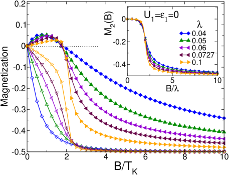
Figure 4: (Color online) Magnetization of dot 1 (empty symbols) and dot 2 (filled symbols) vs scaled magnetic field $B/T_{K}$ at zero temperature for the same parameters as in the main panels of Fig. 3. The dot-1 magnetization $M_{1}$ decreases monotonically from zero over a characteristic field scale that grows with $\lambda$ and approaches $2T_{K}$ for sufficiently large interdot couplings. The dot-2 magnetization $M_{2}$ is of opposite sign to $M_{1}$ for $B\lesssim 2T_{K}$, pointing to the dominance of the antiferromagnetic interdot exchange interaction over this field range. Both dots become fully polarized antiparallel to the field for $B\gg 2T_{K}$. Inset: $M_{2}$ vs $B/\lambda$ for the noninteracting system with the same parameters as in the inset of Fig. 3(a). In contrast to the interacting case, $M_{2}$ decreases monotonically from zero with increasing field.

Figure 4 shows the variation of $M_{1}$ with $B$ for the same model parameters used in Fig. 2. As expected, $M_{1}$ decreases monotonically from zero over a field scale that grows with $\lambda$. For small $\lambda$, this scale is identical to that characterizing the initial decrease of $f_{1}$ from 1 [see Fig. 3(a)], while for larger $\lambda$, $|M_{1}|$ grows on the scale $B^{*}$ of the second peak in $f_{1}(B)$. In all cases, dot 1 is essentially fully polarized for $B\gtrsim 2T_{K}$. That the monotonic evolution of $M_{1}$ does not accompany a monotonic decrease in $f_{1}(B)$ is an indication of the importance of the phase factor $\varphi_{1\uparrow}$ on the right-hand side of Eq. (27).

It is difficult to evaluate $\varphi_{1\sigma}$ directly from Eq. (15) using the NRG because this task requires accurate determination of both the real and imaginary parts of $\mathcal{G}_{\sigma}(\omega,0)$ for all $\omega<0$, whereas the NRG is well-suited only to compute $\mathrm{Im}\,\mathcal{G}_{\sigma}(\omega,0)$ for $|\omega|\ll D$. At particle-hole symmetry, however, one can use Eq. (27) to work backward from the NRG values of $f_{1}$ and $M_{1}$ to find $\varphi_{1\uparrow}=-\varphi_{1\downarrow}$. Fig. 3(b) plots the phase obtained in this manner from the data in Figs. 3(a) and 4. For all values of $\lambda$, $\varphi_{1\uparrow}$ is zero at $B=0$ (as expected) and approaches $\pi$ at large field values. For larger values of $\lambda$, $\varphi_{1\uparrow}$ shows a pronounced kink at $B=B^{*}$. This kink is related, via Eq. (27), to the peak in $f_{1}(B)$ at $B^{*}$, since $M_{1}(B)$ is a smooth function of $B$ (as shown in Fig. 4).

Figure 4 also plots the field dependence of the dot-2 magnetization. The fact that $M_{2}$ is of opposite sign to $M_{1}$ for $B\lesssim 2T_{K}$ indicates that the interactions in dot 1 combine with the interdot hopping to yield a dominant antiferromagnetic interdot exchange interaction. Over this range of $B$, it appears that the system minimizes its energy by first aligning the partially Kondo-screened magnetic moment of the strongly interacting dot 1 along the direction favored by the field, and then orienting the less-developed moment on dot 2 to minimize the interdot exchange energy even at a cost in Zeeman energy. The data show that this tendency becomes weaker for stronger interdot couplings, presumably because the interdot exchange $\sim\lambda^{2}$ grows more slowly than the energy scale $T_{K}$ for breaking the Kondo singlet. For all values of $\lambda$, once $B\gtrsim 2T_{K}$, the Zeeman field has largely destroyed the Kondo effect, and both dots are fully polarized for $B\gg 2T_{K}$.

One can gain further insight into the results presented in Figs. 3 and 4 by considering the limit where both dots are noninteracting. Equations (19) and (27) hold equally well for interacting and noninteracting problems. However, the case $U_{1}=U_{2}=0$ offers the advantage that $A_{1}(0,0)$ can also be calculated directly from the imaginary part of

$$\mathcal{G}_{1\sigma}^{0}(\omega,T)=\frac{1}{\omega+i0^{+}-\varepsilon_{1\sigma}-\Sigma_{\sigma}^{0}(\omega,T)},$$ (29)

where at zero temperature the noninteracting self-energy is

$$\Sigma_{\sigma}^{0}(\omega,0)=[(\omega-\varepsilon_{2\sigma})/\Delta_{2}-i]\Delta_{\sigma}(\omega),$$ (30)

giving

$$A_{1\sigma}(0,0)=\frac{1}{\pi}\,\frac{\Delta_{\sigma}(0)}{[\varepsilon_{2\sigma}\Delta_{\sigma}(0)/\Delta_{2}-\varepsilon_{1\sigma}]^{2}+[\Delta_{\sigma}(0)]^{2}}.$$ (31)

The hybridization-weighted spin-average of $A_{1\sigma}(0,0)$ satisfies

$$f_{1}(B)=\frac{1}{2}\sum_{\sigma}\frac{1}{1+(e_{2\sigma}-e_{1\sigma})^{2}},$$ (32)

where $e_{1\sigma}=\varepsilon_{1\sigma}/\Delta_{\sigma}(0)$ and $e_{2\sigma}=\varepsilon_{2\sigma}/\Delta_{2}$. It should be noted that $e_{1\sigma}$ depends on $B$ both through the Zeeman shift of $\varepsilon_{1}$ and the value of $\Delta_{\sigma}(0)=\Delta_{0}(-{\textstyle\frac{1}{2}}\sigma B)$. From Eq. (32) it is apparent that $f_{1}(B)$ attains its maximum value of $1$ only if $e_{2\sigma}=e_{1\sigma}$ for both spin orientations, a condition that can be satisfied only for $\varepsilon_{1}=\varepsilon_{2}=0$ and either $B=0$ or (if $\lambda>\Delta_{2}$) $B=B^{*}=2\sqrt{\lambda^{2}-\Delta_{2}^{2}}$. For $\varepsilon_{1}\neq 0$ and/or $\varepsilon_{2}\neq 0$, $f_{1}(B)$ may have zero, one or two maxima at nonzero fields, but $f_{1}<1$ for all $B$. These observations are consistent with the conclusion drawn from the Friedel sum rule that $f_{1}=1$ is likely to be achieved only under conditions of strict particle-hole symmetry.

The inset of Fig. 3(a) illustrates the field variation of $f_{1}$ for the particle-hole-symmetric case $U_{1}=\varepsilon_{1}=\varepsilon_{2}=0$, with all other parameters as in the main panel. For each of the $\lambda$ values illustrated (all of which lie in the range $\lambda>\Delta_{2}$), $f_{1}$ reaches 1 at a magnetic field consistent with the value $B^{*}$ derived in the previous paragraph. Note that $B^{*}$ approaches $2\lambda$ from below in the limit of strong interdot coupling. The inset of Fig. 4 plots $M_{2}$ vs $B$ for the same noninteracting cases. For each $\lambda$ value, $|M_{2}|$ shows a purely monotonic field variation, with a rather sudden increase around $B\simeq 2\lambda$, a behavior that is mimicked in the interacting system for $B\simeq 2T_{K}$, especially at large interdot coupling $\lambda$. The variation of the interacting $f_{1}$ and $M_{2}$ for $B\gtrsim 2T_{K}$ seen in the main panels of Figs. 3(a) and 4, particularly for the larger values of $\lambda$, may perhaps be interpreted as a many-body analog of the noninteracting behavior in the insets, with $T_{K}$ serving as a renormalized value of the single-particle scale $\lambda$.

V Electrical Conductance

While the spectral functions discussed in the preceding sections are difficult to access directly in experiments, they may be probed indirectly through transport measurements. In this section, we show that the zero-bias electrical conductance through the double-dot device contains clear signatures of the nonuniversal variation of $\pi\Delta(0)\,A_{1}(0,0)$ with applied field. In particular, we demonstrate the feasibility of generating currents through the system that are strongly or even completely spin-polarized.

Although the linear conductance is given most compactly by Eq. (7), it is also useful to express $G$ in terms of the Green’s function for the interacting dot 1 by combining Eq. (5) with a generalization of Eq. (6) in Ref. Dias2, to include the Zeeman field:

$$\!\!\!\!- \mathrm{Im}\,\mathcal{T}_{\sigma}(\omega,T)$$

$$\;\;=[1-2\pi\Delta_{2}\rho_{2\sigma}(\omega)]\,\pi\Delta_{\sigma}(\omega)\,A_{1\sigma}(\omega,T)+\pi\Delta_{2}\rho_{2\sigma}(\omega)$$

$$\qquad+2\pi(\omega-\varepsilon_{2\sigma})\,\rho_{2\sigma}(\omega)\,\Delta_{\sigma}(\omega)\>\mathrm{Re}\,\mathcal{G}_{1\sigma}(\omega,T),$$ (33)

where $\rho_{2\sigma}(\omega)=\rho_{2}(\omega-{\textstyle\frac{1}{2}}\sigma g\mu_{B}B)$, with $\rho_{2}(\omega)$ and $\Delta_{\sigma}(\omega)$ as defined in Eqs. (23) and (24), respectively. The term $\pi\Delta_{2}\rho_{2\sigma}(\omega)$ describes the bare transmission through dot 2 in the absence of dot 1, while the remaining terms represent additional contributions arising from conductance paths that include dot 1. In the special case $\lambda=0$ where the latter contributions necessarily vanish, the zero-temperature conductance reduces to

$$G_{\text{one-dot}}(T=0)=\frac{G_{0}}{2}\sum_{\sigma}\frac{1}{1+e_{2\sigma}^{2}},$$ (34)

where $e_{2\sigma}$ is defined after Eq. (32).

V.1 Zero temperature

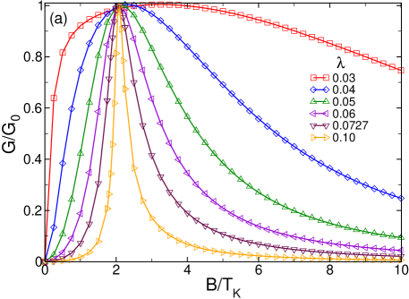
Figure 5: (Color online) Linear conductance $G$ vs scaled magnetic field $B/T_{K}$ at zero temperature for the same parameters as in the main panels of Fig. 3. $G$ rises from zero over the same characteristic field scale as governs the rise of $|M_{1}|$ in the main panel of Fig. 4.

Figure 5 plots the zero-temperature linear conductance $G$ as a function of scaled field $B/T_{K}$ for the same parameters used in Fig. 3. For the case $\varepsilon_{2}=0$ considered here, the conductance of dot 2 alone, $G_{\text{one-dot}}(T=0)=G_{0}[1+(B/2\Delta_{2})^{2}]^{-1}$, decreases monotonically from $G_{0}$ as the Zeeman field detunes the dot level from the Fermi energy of the leads. For any $\lambda\neq 0$ and $B=0$, Kondo correlations in dot 1 produce zero conductance through the double-dot system.Dias2 Figure 5 shows that with increasing field, the double-dot conductance initially increases, then peaks at its maximum possible value $G=G_{0}$ for a field value $B^{**}$ that for large $\lambda$ approaches $2T_{K}$ from above, and finally drops back toward zero for $B\gg B^{**}$. The field $B^{**}$ is distinct from that characterizing the peak in $\pi\Delta(0)\,A_{1}(0,0)$. In general $B^{*}<2T_{K}<B^{**}$, but these three scales converge for $\lambda\gg\Delta_{2}$.

The initial rise in $G$ with increasing field can be attributed to the progressive suppression of the Kondo effect allowing dot 1 to become partially polarized and reducing the destructive interference between the Kondo resonance and the dot-2 resonant state. This change takes place—in agreement with the evolution seen in $\pi\Delta(0)\,A_{1}(0,0)$ and $M_{1}$—over a field scale that increases with $\lambda$ but is not just a constant multiple of $T_{K}$. By the point that the conductance reaches its peak at $B=B^{**}$, the interchannel interference is clearly constructive since Eq. (34) would predict a much lower conductance for dot 2 alone. At still larger fields, the destruction of the Kondo resonance becomes complete and the dot-2 resonance is shifted far from the Fermi level, leading to a decrease of the conductance.

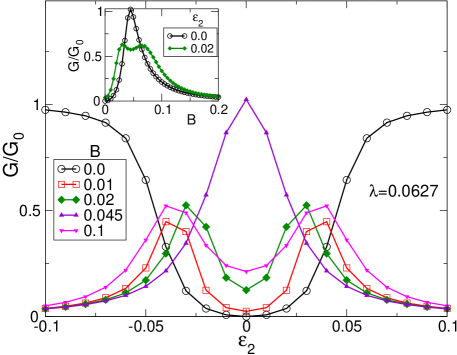
Figure 6: (color online) Linear conductance $G$ vs dot-2 level energy $\varepsilon_{2}$ at zero temperature for $U_{1}=-2\varepsilon_{1}=0.5$, $\lambda=0.0627$, and five different magnetic field values. The conductance is symmetric about the point $\varepsilon_{2}=0$ of particle-hole symmetry. In nonzero fields, $G$ peaks at some $|\varepsilon_{2}|\neq 0$, apart from the special case $B=B^{**}\simeq 0.045\simeq 2T_{K}$, for which the conductance is maximal at $\varepsilon_{2}=0$ (as already seen in Fig. 5). Inset: Conductance vs magnetic field $B$ for $\varepsilon_{2}=0$ and $0.02$.

Figure 6 illustrates aspects of the transport away from particle-hole symmetry. The main panel shows the variation of the $T=0$ linear conductance at several different fixed magnetic fields as the value of $\varepsilon_{2}$ is swept by varying the voltage on a plunger gate near dot 2. For $B=0$, the conductance increases from zero at $\varepsilon_{2}=0$ and approaches $G_{0}$ for $|\varepsilon_{2}|\gg\Delta_{2}$ as the dot-2 resonance is tuned away from the Fermi energy, thereby permitting perfect conduction through the Kondo many-body resonance. For fixed $B>0$, competition between Zeeman splitting of the dot-2 resonance and partial destruction of the Kondo effect leads in most cases to an initial rise in $G$ for small $|\varepsilon_{2}|$ followed by a fall-off at larger $|\varepsilon_{2}|$. As the magnetic field increases from zero, the conductance peaks initially move to smaller $|\varepsilon_{2}|$, then merge into a single peak at $G=G_{0}$ for $B=B^{**}\simeq 0.045$ for the case $\lambda=0.0627$ here, before separating and moving to larger $|\varepsilon_{2}|$ as $B$ moves to still higher values. Thus $B^{**}$ can in principle be located as the only field at which $G$ has a single peak vs $\varepsilon_{2}$.

The inset to Figure 6 compares the field variation of $G(T=0)$ for $\varepsilon_{2}=0$ and for $\varepsilon_{2}=0.02$. It is only in the former case (i.e., under conditions of strict particle-hole symmetry), that the conductance has a single peak vs $B$ and attains $G=G_{0}$, whereas for $\varepsilon_{2}\neq 0$ one finds a pair of peaks at $G<G_{0}$. The presence of a single peak under field sweeps can therefore be used to identify the particle-hole-symmetric point in experiments.

To better understand these results, we again turn to the noninteracting case $U_{1}=0$, where the linear conductance can be calculated by substituting the noninteracting Green’s function given by Eqs. (29) and (30) for the full Green’s function $\mathcal{G}_{\sigma}$ in Eq. (V). At $T=0$, this results in a conductance contribution

$$G=\sum_{\sigma}G_{\sigma}={\textstyle\frac{1}{2}}\,G_{0}\sum_{\sigma}\frac{e_{1\sigma}^{2}}{[1+e_{2\sigma}^{2}][1+(e_{2\sigma}-e_{1\sigma})^{2}]}\,$$ (35)

where $e_{1\sigma}$ and $e_{2\sigma}$ are defined after Eq. (32). Equation (35) correctly reduces to Eq. (34) in the limit $|\varepsilon_{1}|\to\infty$ where dot 1 can play no role in the conductance. At particle-hole symmetry ($\varepsilon_{1}=\varepsilon_{2}=0$), Eq. (35) gives

$$G=G_{0}\frac{[B/2\Delta(0)]^{2}}{[1+(B/2\Delta_{2})^{2}]\{1+[B/2\Delta_{2}-B/2\Delta(0)]^{2}\}}\,$$ (36)

which peaks at $G=G_{0}$ for $B=B^{**}=2\lambda$, a characteristic field greater than the one $B^{*}=2\sqrt{\lambda^{2}-\Delta_{2}^{2}}$ at which $\pi\Delta(0)\,A_{1}(0,0)$ reaches 1. Since we have seen above that $G(T=0)$ for the interacting case at particle-hole symmetry reaches $G_{0}$ for some $B^{**}>2T_{K}>B^{*}$, with $B^{**}\to 2T_{K}$ for large $\lambda$, the field dependence of the conductance reinforces the parallels between the large-$\lambda$ interacting problem and the noninteracting limit, with the many-body scale $T_{K}$ playing the role of a renormalized $\lambda$.

An interesting feature of Eq. (35) is that it predicts conduction contributions $G_{\uparrow}\neq G_{\downarrow}$ when particle-hole symmetry and time-reversal symmetry are both broken. In particular, for $\varepsilon_{1}>0$ (or $\varepsilon_{1}<0$), the conductance polarization measured by

$$\eta=\frac{G_{\uparrow}-G_{\downarrow}}{G_{\uparrow}+G_{\downarrow}}$$ (37)

grows from $\eta=0$ for $B=0$ to reach $\eta=1$ (or $\eta=-1$) for $B=2|\varepsilon_{1}|$, at which field $\varepsilon_{1\downarrow}=0$ (or $\varepsilon_{1\uparrow}=0$), before decreasing toward zero for still larger fields. By contrast, keeping $\varepsilon_{1}=0$ but allowing $\varepsilon_{2}\neq 0$ results in variation of $\eta$ with field, but does not allow one to achieve perfect polarization of the conductance.

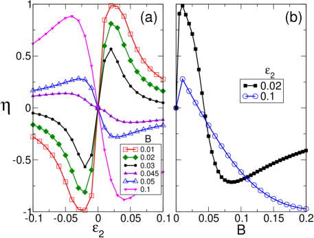
Figure 7: (Color online) Conductance spin-polarization $\eta$ (a) vs dot-2 level energy $\varepsilon_{2}$ at six fixed magnetic fields $B$, and (b) vs $B$ for two values of $\varepsilon_{2}$. All data are for $U_{1}=-2\varepsilon_{1}=0.5$, $\lambda=0.0627$, and zero temperature. In (a), $\eta$ is odd about the point $\varepsilon_{2}=0$ of particle-hole symmetry. Complete spin polarization of the conductance is achieved in the case $B=0.01$. Panel (b) shows a strong, nonuniversal variation of $\eta$ with $B$ for different values of $\varepsilon_{2}$.

Spin-dependent conductance is also exhibited when dot 1 has strong interactions. Figure 7(a) shows the variation of $\eta$ with the dot 2 level energy $\varepsilon_{2}$ in different fields $B\neq 0$ for a symmetric dot 1 ($U_{1}=-2\varepsilon_{1}$) and fixed $\lambda$. The conductance spin-polarization is odd about the point $\varepsilon_{2}=0$ of particle-hole symmetry where the condition $A_{1\uparrow}(\omega,T)=A_{1\downarrow}(-\omega,T)$ ensures [via Eq. (7)] that $\eta=0$. For fields $B\lesssim 2T_{K}\simeq 0.042$, $\eta$ has the same sign as $\varepsilon_{2}$, whereas for $B\gtrsim 2T_{K}$, $\eta$ and $\varepsilon_{2}$ have opposite signs. For each field value, $|\eta|$ peaks at a nonzero value of $|\varepsilon_{2}|$. One sees that a field $B=0.01$ combines with a level energy $|\varepsilon_{2}|\simeq 0.025$ to achieve complete destructive interference of the conduction for one spin species, allowing passage only of a fully spin-polarized current through the device. The fact that reaching $|\eta|=1$ in this manner—by varying $\varepsilon_{2}$ while dot 1 is held at particle-hole symmetry ($\varepsilon_{1}=0$)— is impossible to achieve in the noninteracting case $U_{1}=0$ indicates that the interference effects are more complex in the presence of strong interactions.

It is important to emphasize that, in contrast to the maximal conductance value $G_{0}$, the polarization $\eta$ is unaffected by asymmetry between the left and right dot-lead couplings. Complete spin polarization ($|\eta|=1$) can be achieved even in setups where $V_{2L}\neq V_{2R}$.

Figure 7(b) shows the variation of $\eta$ under field sweeps at two different values $\varepsilon_{2}>0$. For each position of the dot-2 level, $\eta$ changes sign at a nonzero $B$. For $\varepsilon_{2}=0.02$, $\eta$ reaches $+1$ at a small field and then dips to nearly $-1$ at a larger field before increasing back toward zero. For $\varepsilon_{2}=0.1$, by contrast, a small positive peak in $\eta$ is followed at larger fields by a dip at (or very close to) $-1$. This nonuniversal behavior reflects the subtlety of the interplay between the field and particle-hole asymmetry in controlling the constructive or destructive interference between transmission of electrons directly through dot 2 and paths involving one or more detours to dot 1.

Similar “spin-filtering” effects in a magnetic field have been investigated previouslyAligia2004 ; Torio2004 in the context of a single-mode wire, coupled near its midpoint via a tunnel junction to a quantum dot (the “side dot”). A number of experiments and models using different geometries for spin-dependent transport have also been reported in the literature.vdWiel ; SpinPolRMP Reference Torio2004, showed that conductance polarizations $\eta=1$ and $\eta=-1$ (in the language of the present paper) occur at values of the dot energy $\varepsilon_{d}(\eta=1)$ and $\varepsilon_{d}(\eta=-1)$ differing by a large scale exceeding the dot Coulomb interaction strength $U$. Thus, the change in gate voltage needed to switch the polarizations is so large that all traces of the Kondo effect are suppressed. These behaviors should be contrasted with those found here, where the $\varepsilon_{2}$ values that lead to $\eta=\pm 1$ differ only by an energy of order $\Delta_{2}$ (much smaller than $U_{1}$). What is more, the complete spin filtering achieved in our setup depends crucially on the presence of Kondo many-body correlations. This point will become particularly clear in the next section, where we consider the effect of nonzero temperatures. Reference Aligia2004, considered a side-coupled quantum dot in regime of much smaller Kondo temperatures. In contrast to our results for double quantum dots, complete polarization of the conductance was reported to occur quite generically due to a mechanism very similar to that we find in the noninteracting limit $U_{1}=0$ described by Eq. (35).

V.2 Nonzero temperatures

To this point, only zero-temperature results have been presented. This subsection addresses the effect of finite temperatures on the zero-bias conductance $G$ and its spin polarization $\eta$. Throughout the discussion, temperatures are expressed as multiples of a characteristic many-body scale $T_{K0}=0.021$, the system’s Kondo temperature for $\varepsilon_{2}=0$, $B=0$, and the representative value $\lambda=0.0627$ that we have used in all our $T>0$ calculations.

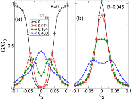
Figure 8: (Color online) Linear conductance $G$ vs dot-2 level position $\varepsilon_{2}$ for $U_{1}=-2\varepsilon_{1}=0.5$ and $\lambda=0.0627$ at four temperatures $T$ for (a) $B=0$, and (b) $B=0.045\simeq 2T_{K0}$. Temperatures are expressed as multiples of $T_{K0}=0.021$.

Figure 8 plots $G$ vs $\varepsilon_{2}$ for $\lambda=0.0627$ in fields $B=0$ (panel a) and $B\simeq B^{**}\simeq 2T_{K0}$ (panel b). For $B=0$, the effect of increasing temperature is a progressive suppression of the Kondo effect and hence of the conductance channel involving the many-body Kondo resonance. As a result, $G$ rises near $\varepsilon_{2}=0$ due to a lessening of the destructive interference between the Kondo channel and the single-particle resonance on dot 2 (discussed above in connection with Fig. 6), but there is a decrease in the conductance at $|\varepsilon_{2}|\gtrsim\Delta_{2}$, which is dominated by transmission through the Kondo channel. This trend results in a conductance peak at some $|\varepsilon_{2}|\neq 0$ for temperatures $0<T\lesssim T_{K0}$, which evolves into a peak centered at $\varepsilon_{2}=0$ for $T\gtrsim T_{K0}$, in which regime transmission is dominated by the single-particle, Lorentzian-like contribution from dot 2.

Figure 8(b) reveals a very different behavior for $B=B^{**}\simeq 2T_{K0}$. As described above, the $T=0$ conductance attains its maximum possible value $G_{0}$ at $\varepsilon_{2}=0$ due to constructive interference between the Kondo and single-particle conductance channels, and $G$ decreases monotonically with increasing $|\varepsilon_{2}|$. Raising the temperature over the range $T\lesssim T_{K0}$ leads to suppression of the Kondo conductance channel but has little effect on the single-particle channel, leading to a decrease in $G$ that is strongest for $\varepsilon_{2}=0$. Once the temperature passes $T_{K0}$, the variation of $G$ with $\varepsilon_{2}$ increasingly reflects the field splitting of the dot-2 energy level, with peaks centered at $\varepsilon_{2}\simeq\pm{\textstyle\frac{1}{2}}B$.

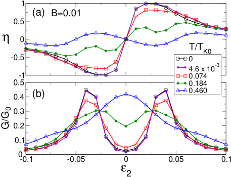
Figure 9: (Color online) (a) Conductance spin-polarization $\eta$, and (b) conductance $G$ vs dot-2 level energy $\varepsilon_{2}$ at different temperatures for $U_{1}=-2\varepsilon_{1}=0.5$, $\lambda=0.0627$, and $B=0.01$. Temperatures are expressed as multiples of $T_{K0}=0.021$.

The influence of temperature on the spin polarization of the conductance is shown in Fig. 9(a), which focuses on the case $B=0.01$ that we know from Fig. 7 yields full spin polarization ($\eta=\pm 1$) at zero temperature for $\varepsilon_{2}\simeq\pm 0.025$. As $T$ increases from zero, the peak spin polarization is lowered, presumably due to a combination of two effects: (i) a reduction in the destructive interference between the Kondo and single-particle conduction channels for one spin species $\sigma$ leading to an increase in $-\mathrm{Im}\,\mathcal{T}_{\sigma}(\omega=0,T)$ entering Eq. (5); and (ii) thermal broadening of $-\partial f/\partial\omega$ in Eq. (5) leading to sampling of $\omega$ values having nonzero $-\mathrm{Im}\,\mathcal{T}_{\sigma}(\omega,T=0)$. At higher temperatures, $T\simeq T_{K0}$, the suppression of the Kondo conductance channel unmasks oscillations in $\eta$ vs $\varepsilon_{2}$ that result from shifts in the spin-resolved energy levels in dot 2. These oscillations are much less pronounced than the polarization variations at lower temperatures and the maximum values of $|\eta|$ are about an order of magnitude smaller than those obtained in the Kondo regime.

Figure 9(b) plots the total conductance $G$ vs $\varepsilon_{2}$ corresponding to each of the $\eta$ vs $\varepsilon_{2}$ traces in Fig. 9(a). There is a close correlation (although not a perfect match) between the $\varepsilon_{2}$ values of the peaks in $G$ and of those in $|\eta|$. This suggests that measurements of the total conductance can provide a useful starting point for experiments seeking to optimize the system’s spin-filtering performance.

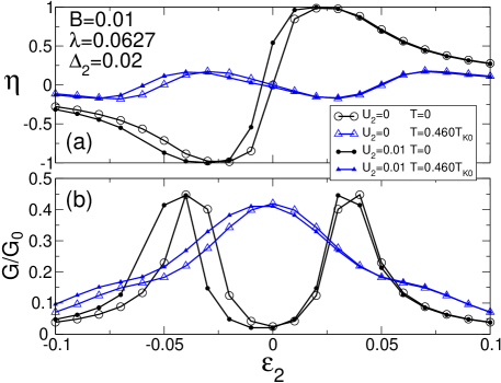
Figure 10: (Color online) Effect of a nonzero dot-2 interaction ($U_{2}>0$) on (a) the conductance spin-polarization $\eta$, and (b) the conductance $G$, both plotted vs dot-2 level energy $\varepsilon_{2}$ for the same parameters as in Fig. 9. Open symbols correspond to $U_{2}=0$ and filled symbols to $U_{2}=0.01$. Temperatures are expressed as multiples of $T_{K0}=0.021$.

Although we have focused on the special case $U_{2}=0$, the conductance features described above by no means depend on this condition. In fact, qualitatively similar results are obtained for an interacting dot 2 provided that $U_{2}$ is small compared to the level broadening $\Delta_{2}$. This is illustrated in Fig. 10, which compares the $\varepsilon_{2}$ dependence of the conductance and of its spin-polarization for $U_{2}=0$ (data from Fig. 9) and $U_{2}={\textstyle\frac{1}{2}}\Delta_{2}=0.01$, both for the lowest ($T=0$) and highest ($T=0.460T_{K0}$) temperatures shown in Fig. 9. Apart from a small shift in the point of particle-hole symmetry, which moves from $\varepsilon_{2}=0$ to $\varepsilon_{2}=-{\textstyle\frac{1}{2}}U_{2}$, the other essential features (such as the complete spin polarization at zero temperature) are unaffected by the presence of Coulomb repulsion within dot 2.

VI Conclusions

In this work, we have investigated the effect of an applied magnetic field on a strongly interacting quantum dot side-coupled to external leads via a weakly interacting dot. Our numerical renormalization-group results show that the interplay of electronic interference, the Kondo effect, and Zeeman splitting brings about qualitative changes in the spectral and transport properties of this system. We have found, for instance, that the value of the interacting dot’s zero-temperature spectral function at the Fermi energy does not decay monotonically with increasing field, as it does in single-dot setups. Instead, the presence of the extra energy scale determined by the interdot coupling introduces nonuniversal behavior, and in some cases leads to the appearance of one or two maxima in the Fermi-energy spectral function at nonzero values of $B$. These features can be understood by the presence of a parameter-dependent phase appearing in the Friedel sum rule for energy- and spin-dependent hybridization functions.

One of the signatures of the interplay of site and spin degrees of freedom in this double-dot device is the appearance of spin-polarized currents between the two leads. We have shown that the degree of spin polarization can be tuned up to 100% by changing gate voltages and/or small magnetic fields in the system. These results underscore the flexibility of quantum-dot systems for exploration of novel effects in correlated electron physics.

- (1) D. Goldhaber-Gordon, H. Shtrikman, D. Mahalu, D. Abusch-Magder, U. Meirav, and M. A. Kastner, Nature (London) 391, 156 (1998).
- (2) L. Kouwenhoven and C. Marcus, Phys. World 11, 35 (1998).
- (3) S. M. Cronenwett, T. H. Oosterkamp, and L. P. Kouwenhoven, Science 281, 540 (1998).
- (4) A. C. Hewson, The Kondo Problem to Heavy Fermions (Cambridge University Press, Cambridge, U.K., 1997).
- (5) H. Jeong, A. M. Chang, and M. R. Melloch, Science 293, 2221 (2001).
- (6) J. C. Chen, A. M. Chang, and M. R. Melloch, Phys. Rev. Lett. 92, 176801 (2004).
- (7) N. J. Craig, J. M. Taylor, E. A. Lester, C. M. Marcus, M. P. Hanson, and A. C. Gossard, Science 304, 565 (2004).
- (8) R. M. Potok, I. G. Rau, H. Shtrikman, Y. Oreg and D. Goldhaber-Gordon, Nature 446, 167 (2007).
- (9) A. Hübel, K. Held, J. Weis, and K. v. Klitzing, Phys. Rev. Lett 101, 186804 (2008).
- (10) W. G. van der Wiel, S. De Franceschi, J. M. Elzerman, T. Fujisawa, S. Tarucha, and L. P. Kouwenhoven, Rev. Mod. Phys. 75, 1 (2002).
- (11) V. M. Apel, M. A. Davidovich, E. V. Anda, G. Chiappe, C. A. Büsser, Eur. Phys. J. B 40, 365 (2004).
- (12) C. A. Büsser, G. B. Martins, K. A. Al-Hassanieh, A. Moreo, and E. Dagotto, Phys. Rev. B 70, 245303 (2004).
- (13) P. S. Cornaglia and D. R. Grempel, Phys. Rev. B 71, 075305 (2005).
- (14) Y. Tanaka and N. Kawakami, Phys. Rev. B 72, 085304 (2005).
- (15) R. Žitko and J. Bonča, Phys. Rev. B 73, 035332 (2006).
- (16) Y. Tanaka, N. Kawakami, and A. Oguri, Phys. Rev. B 78, 035444 (2008).
- (17) R. Žitko, Phys. Rev. B 81, 115316 (2010).
- (18) I. L. Ferreira, P. A. Orellana, G. B. Martins, F. M. Souza, and E. Vernek, Phys. Rev. B 84, 205320 (2011).
- (19) Y. Tanaka, N. Kawakami, and A. Oguri, Phys. Rev. B 85, 155314 (2012).
- (20) A. E. Miroshnichenko, S. Flach, and Y. S. Kivshar, Rev. Mod. Phys. 82, 2257 (2010).
- (21) L. G. G. V. Dias da Silva, N. P. Sandler, K. Ingersent, and S. E. Ulloa, Phys. Rev. Lett. 97, 096603 (2006).
- (22) L. G. G. V. Dias da Silva, N. P. Sandler, K. Ingersent, and S. E. Ulloa, Phys. Rev. Lett. 99, 209702 (2007).
- (23) L. G. G. V. Dias da Silva, K. Ingersent, N. P. Sandler, and S. E. Ulloa, Phys. Rev. B 78, 153304 (2008).
- (24) L. Vaugier, A. A. Aligia, and A. M. Lobos, Phys. Rev. Lett. 99, 209701 (2007).
- (25) N. Andrei, Phys. Rev. Lett. 45, 379 (1980).
- (26) W. Hofstetter, Phys. Rev. Lett. 85, 1508 (2000).
- (27) T. A. Costi, Phys. Rev. Lett. 85, 1504 (2000).
- (28) D. E. Logan and N. L. Dickens, J. Phys. Condens. Matter 13, 9713 (2001).
- (29) K. G. Wilson, Rev. Mod. Phys. 47, 773 (1975); H. R. Krishna-murthy, J. W. Wilkins, and K. G. Wilson, Phys. Rev. B 21 1003 (1980); R. Bulla, T. A. Costi, T. Pruschke, Rev. Mod. Phys. 80, 395 (2008).
- (30) L. I. Glazman and M. E. Raikh, JETP Lett. 47, 452 (1988); T. K. Ng and P. A. Lee, Phys. Rev. Lett. 61, 1768 (1988).
- (31) D. N. Zubarev, Usp. Fiz. Nauk 71, 71 (1960).
- (32) Y. Meir and N. S. Wingreen, Phys. Rev. Lett. 68, 2512 (1992).
- (33) D. E. Logan, C. J. Wright, and M. R. Galpin, Phys. Rev. B 80, 125117 (2009).
- (34) R. Bulla, T. A. Costi, and D. Vollhardt, Phys. Rev. B 64, 045103 (2001).
- (35) S. Schmitt, and F. B. Anders, Phys. Rev. B 83, 197101 (2011); R. Zitko, Phys. Rev. B 84, 085142 (2011).
- (36) J. Martinek, M. Sindel, L. Borda, J. Barnaś, J. König, G. Schön, and J. von Delft, Phys. Rev. Lett. 91, 247202 (2003).
- (37) L. Vaugier, A. A. Aligia, and A. M. Lobos, Phys. Rev. B 76, 165112 (2007).
- (38) D. C. Langreth, Phys. Rev. 150, 516 (1966).
- (39) C. J. Wright, M. R. Galpin, and D. E. Logan, Phys. Rev. B 84, 115308 (2011).
- (40) A. A. Aligia, and L. A. Salguero, Phys. Rev. B 70, 075307 (2004).
- (41) M. E. Torio, K. Hallberg, S. Flach, A. E. Miroshnichenko, and M. Titov, Eur. Phys. J. B 37, 399 (2004).