The strong coupling from tau decays without prejudice

Abstract

We review our recent determination of the strong coupling $\alpha_{s}$ from the OPAL data for non-strange hadronic tau decays. We find that $\alpha_{s}(m^{2}_{\tau})=0.325\pm 0.018$ using fixed-order perturbation theory, and $\alpha_{s}(m^{2}_{\tau})=0.347\pm 0.025$ using contour-improved perturbation theory. At present, these values supersede any earlier determinations of the strong coupling from hadronic tau decays, including those from ALEPH data.

1. Figure 1 shows a number of recent determinations of the strong coupling, $\alpha_{s}(m^{2}_{\tau})$, from hadronic tau decays. The two values at the top are recent determinations [1] from OPAL data [2], and have signficantly larger errors than all the other determinations shown. The reason for these larger errors is twofold: (1) errors in the non-perturbative part of the sum rules used in order to extract $\alpha_{s}(m^{2}_{\tau})$ have been systematically underestimated in earlier works; (2) all other values shown in Fig. 1 used ALEPH data, with correlations in which the effects of unfolding the spectrum have inadvertently been omitted [3]. Here we give a brief overview of our analysis [1, 4], comparing it with the standard approach used in for instance Ref. [5]. We note that for the values shown in Fig. 1 only those of Refs. [1, 5, 6] are based directly on data; all others used estimates for the non-perturbative part from Ref. [5].

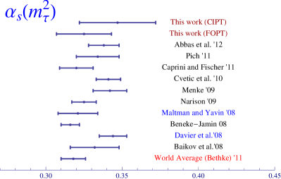
Figure 1: Recent values for $\alpha_{s}(m^{2}_{\tau})$ from hadronic tau decays. For references, see Ref. [7].

2. All tau-based determinations of $\alpha_{s}(m^{2}_{\tau})$ start from the sum rule

$$\int_{0}^{s_{0}}\!\!\!ds\;w(s)\;\rho_{\rm exp}(s) \!=\! -\frac{1}{2\pi i}\oint_{|z|=s_{0}}\!\!\!\!\!dz\;w(z)\;\Pi_{\rm OPE}(z)$$ (1)

$$-\frac{1}{\pi}\int_{s_{0}}^{\infty}\!\!\!ds\;w(s)\;{\rm Im}\;\Pi_{\rm DV}(s)\ ,$$

in which $w(s)$ is a polynomial weight, $\rho_{\rm exp}(s)$ is the inclusive, non-strange spectral function taken from experiment, $\Pi_{\rm OPE}(z)$ is the operator product expansion (OPE) expression for the non-strange flavor off-diagonal vacuum polarization with perturbation theory constituting the (dimension $D=0$) dominant part, and

$$\Pi_{\rm DV}(z)\equiv\Pi_{\rm QCD}(z)-\Pi_{\rm OPE}(z)$$ (2)

the correction for using $\Pi_{\rm OPE}(z)$ instead of the (unknown) exact $\Pi_{\rm QCD}(z)$. It is important to include an estimate for the duality-violating (DV) term in Eq. (1), because duality violations are not small near the Minkowski axis in the complex $z$ plane, from which the integral on the left-hand side of Eq. (1) originates. In more physical terms, the OPE does not capture the hadronic resonances which are clearly visible in the experimental spectrum $\rho_{\rm exp}(s)$.

While the perturbative part of $\Pi_{\rm OPE}(z)$ is known to 4th order in $\alpha_{s}(m^{2}_{\tau})$ [8] and the condensate corrections are expected to give a good estimate for non-perturbative corrections for $|z|=s_{0}$ large and away from the Minkowski axis, we need to use a model in order to estimate the effects of the DV term in Eq. (1). Based on an extensive study of models for the resonances seen in $\rho_{\rm exp}(s)$, we have used the ansatz (see Ref. [4] and references therein)

$$\frac{1}{\pi}\;{\rm Im}\;\Pi_{\rm DV}(s)=e^{-\gamma s-\delta}\sin{(\alpha+\beta s)}\ .$$ (3)

3. This very brief overview of the theory (for more details and references, see Refs. [4, 1]) makes it possible to compare the “standard” analysis of Refs. [2, 5]) with ours. In the standard analysis:

• It is assumed that duality violations can be neglected if one uses “pinched” weights $w(s)$, which always include factors $(1-s/s_{0})^{n}$, with $n=2$ or $n=3$. Such weights are thus necessarily polynomials of at least degree 2.

• One chooses $s_{0}=m_{\tau}^{2}$, and 5 pinched weights of degrees 3 to 7, generating 5 data points, to which one fits 4 parameters, $\alpha_{s}(m^{2}_{\tau})$ and the dimension 4, 6 and 8 OPE condensates. We note that three of the five employed moments have problematic perturbative behavior [9].

• This assumes that OPE condensates of dimension 10 through 16 vanish, because a term of order $s^{k}$ in the weight $w(s)$ picks out a term of dimension $D=2k+2$ in the OPE. This assumption was shown to be not self-consistent in Ref. [6].

In contrast, in our work:

• Our main fit uses the data for the vector channel, and the weight $w=1$, for which no OPE terms beyond perturbation theory contribute.

• We let $s_{0}$ vary over an interval $[s_{min},m_{\tau}^{2}]$, with $s_{min}$ determined by the quality and stability of the fit; typically, $s_{min}\approx 1.5$ GeV². This provides more (correlated) data compared to choosing $s_{0}=m_{\tau}^{2}$.

• We include duality violations. Our main fit thus has 5 parameters, $\alpha_{s}(m^{2}_{\tau})$ and the 4 parameters of Eq. (3) for the vector channel.

• We check consistency using also the axial-channel data, and adding other weights up to degree 3 (always retaining all required terms in the OPE, i.e., to dimension 8.)

For more discussion of our strategy, we refer to Ref. [4].

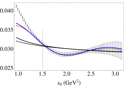
Figure 2: Vector channel fit of Eq. (1) with $w=1$ using OPAL data. CIPT fits are shown in red (dashed) and FOPT in blue (solid). The (much flatter) black curves represent the OPE parts of the fits. The vertical dashed line indicates the location of $s_{min}$.

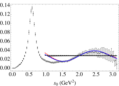
Figure 3: Spectral function predicted by the fit of Fig. 2, compared with OPAL data. CIPT fits are shown in red (dashed) and FOPT in blue (solid). The (much flatter) black curves represent the OPE parts.

Figure 2 shows the result of a fit to the vector channel with weight $w=1$ and $s_{min}=1.5$ GeV², with all correlations between the data taken into account. This fit leads to (FOPT = fixed-order perturbation theory, CIPT = contour-improved perturbation theory)

$$\alpha_{s}(m_{\tau}^{2})\!\!\! = \!\!\!0.307\pm 0.018\pm 0.004\pm 0.005\ ({\rm FOPT})\,,$$

$$= \!\!\!0.322\pm 0.025\pm 0.004\pm 0.005\ ({\rm CIPT})\ ,$$

$$e^{-\delta}\!\!\! = \!\!\!0.02\pm 0.01\ .$$

The value of $\chi^{2}$ for this fit is 0.36 per degree of freedom. The first error is the fit error, the second gives an indication of the stability with respect to varying $s_{min}$, and the third estimates the effect of truncating perturbation theory. From the result for $e^{-\delta}$ as well as from Figs. 2 and 3 it is clear that duality violations have to be taken into account. As mentioned above, and explained in detail in Ref. [4], one may attempt to suppress duality violations by using pinched weights, but at the price of not ignoring terms in the OPE of dimension up to 16 if the weights of the standard analysis are employed. One should then worry, however, whether the OPE converges to such high order for $s_{0}\in[s_{min},m_{\tau}^{2}]$.

We have carried out a number of consistency checks:

• Fits with weights $w=1$, $1-(s/s_{0})^{2}$ and $(1-s/s_{0})^{2}(1+2s/s_{0})$ and also including axial data lead to results completely consistent with Eq. (The strong coupling from tau decays without prejudice). These moments are preferred for their perturbative behavior [9].

• The first and second Weinberg sum rules, as well as the sum rule for the electromagnetic pion mass difference are satisfied within errors.

• Our fits describe the non-strange hadronic tau-decay branching fraction $R_{V+A,ud}(s_{0})$ extremely well for $s_{0}$ above about 1.3 GeV².

The values found originally by OPAL are [2]:

$$\alpha_{s}(m_{\tau}^{2}) = 0.324\pm 0.014\quad({\rm FOPT})\ ,$$

$$= 0.348\pm 0.021\quad({\rm CIPT})\ .$$

We find central values about $0.02$ lower on the same data, and conclude that OPAL errors were underestimated. In particular, errors due to non-perturbative effects are at least as large as the difference between CIPT and FOPT.

4. The 1998 OPAL spectral functions were constructed as a sum over all exclusive modes normalized with the 1998 PDG values of the branching fractions. In Ref. [1], we applied the analysis of Ref. [4] to rescaled OPAL data obtained by instead using current branching fractions from HFAG [10]. For the vector channel, the rescaling factor is shown in Fig. 4.

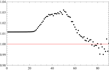
Figure 4: Ratio of the vector-channel OPAL data using HFAG branching fractions and the original OPAL data using 1998 PDG branching fractions. The horizontal axis labels the bins.

In addition, we also carried out a Markov-chain Monte Carlo analysis of the rescaled data in order to explore the $\chi^{2}$ distribution as a function of the parameters $\alpha_{s}(m^{2}_{\tau})$ and those of Eq. (3) in more detail. This distribution forms a five-dimensional landscape, since it is a function of 5 parameters. Cross sections of the full landscape are shown in Fig. 5: in the top figure we show the Monte-Carlo generated $\chi^{2}$ distribution projected onto the $\alpha_{s}$–$\chi^{2}$ plane; in the bottom figure, we show the projection onto the $\alpha_{s}$–$\delta_{V}$ plane.

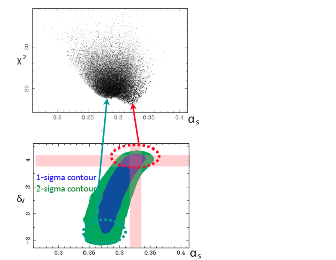
Figure 5: Monte-Carlo analysis of the $\chi^{2}$ distribution for the fit of Eq. (1) with $w=1$ to the vector channel for the rescaled OPAL data. $V$ stands for “vector channel.”

We see that the $\chi^{2}$ distribution corresponds to a rather complicated landscape. The fit appears to allow for two different minima, one with $\delta_{V}\approx 4$ and one with $\delta_{V}\approx-2$. As can be seen in the lower figure, these two minima are not well separated, and the value of $\chi^{2}$ per degree of freedom is reasonable for each minimum.

While the absolute minimum is at $\delta_{V}\approx 4$, clearly we need physical input in order to arrive at a value of $\alpha_{s}$ which is more precise than a value in the range 0.27–0.35 or so that would follow from the top figure. The model developed in Ref. [11] favors

$$\delta_{V}\approx-\log{\frac{F_{\rho}^{2}}{M_{\rho}^{2}}}\approx 4.2\ ,$$ (6)

which leads us to choose the absolute minimum of the $\chi^{2}$ distribution as the preferred value, and consider the other minimum unphysical. With this choice, we find

$$\alpha_{s}(m_{\tau}^{2}) = 0.325\pm 0.018\quad({\rm FOPT})\ ,$$

$$= 0.347\pm 0.025\quad({\rm CIPT})\ .$$

While the central values are virtually the same as those of Eq. (The strong coupling from tau decays without prejudice), this is purely accidental. Moreover, as before, the errors are larger, because of non-perturbative effects. Indeed, if we define $\delta^{\rm NP}$ by

$$R_{V+A,ud}=N_{c}|V_{ud}|^{2}\left(1+\delta^{pert.th.}+\delta^{\rm NP}\right)\ ,$$ (8)

we find that

$$\delta^{\rm NP} = -0.004\pm 0.012\quad(\mbox{FOPT})\ ,$$

$$= -0.002\pm 0.012\quad(\mbox{CIPT})\ .$$

This is to be compared with $\delta^{\rm NP}=-0.0059\pm 0.0014$ from the standard analysis [5, 12]. Our error on $\delta^{\rm NP}$ is an order of magnitude larger, because non-perturbative effects have been treated systematically in our analysis.

5. We presented a new analysis of hadronic tau decays, yielding a new value for the strong coupling, $\alpha_{s}$, at the tau mass, with a larger error than found in previous analyses. Earlier values were all based on the standard analysis summarized in Sec. 3, and, moreover, on the incomplete ALEPH data. Therefore, we believe that our values should be taken as superseding all earlier values for $\alpha_{s}$ from hadronic tau decays.

As we saw in Sec. 4, fits to OPAL data are at the very edge of what is statistically possible. This is not a flaw of the analysis, but appears to be the best one can expect based on the OPAL data. In Ref. [1], we investigated what would happen with the $\chi^{2}$ distribution shown in Fig. 5 if the errors are reduced by a factor 2 or 3. We found that the degeneracy shown in Fig. 5 disappears. Therefore, we expect that a much more stringent test of the sum-rule analysis of hadronic tau decays would be possible if inclusive spectral functions were made available from the BaBar or Belle data.

Acknowledgements We would like to thank M. Beneke, C. Bernard, A. Höcker, M. Martinez, and R. Miquel for discussions, and S. Banerjee and S. Menke for help with understanding the HFAG analysis and OPAL data, respectively. DB is supported by the Alexander von Humboldt Foundation, and MG in part by the US Dept. of Energy, and in part by the Spanish Ministerio de Educación, Cultura y Deporte, under program SAB2011-0074. MJ and SP are supported by CICYTFEDER-FPA2008-01430, FPA2011-25948, SGR2009-894, the Spanish Consolider-Ingenio 2010 Program CPAN (CSD2007-00042). AM was supported in part by NASA through Chandra award No. AR0-11016A. KM is supported by the Natural Sciences and Engineering Research Council of Canada.

References

- [1] D. Boito et al., Phys. Rev. D 85, 093015 (2012) [arXiv:1203.3146 [hep-ph]].
- [2] K. Ackerstaff et al. [OPAL Collaboration], Eur. Phys. J. C 7 (1999) 571 [arXiv:hep-ex/9808019].
- [3] D. Boito et al., arXiv:1011.4426 [hep-ph].
- [4] D. Boito et al., Phys. Rev. D84, 113006 (2011) [arXiv:1110.1127 [hep-ph]].
- [5] S. Schael et al. [ALEPH Collaboration], Phys. Rept. 421, 191 (2005) [arXiv:hep-ex/0506072]; M. Davier et al., Eur. Phys. J. C56, 305 (2008) [arXiv:0803.0979 [hep-ph]].
- [6] K. Maltman, T. Yavin, Phys. Rev. D78, 094020 (2008) [arXiv:0807.0650 [hep-ph]].
- [7] S. Bethke, arXiv:1210.0325 [hep-ex].
- [8] P. A. Baikov, K. G. Chetyrkin, J. H. Kühn, Phys. Rev. Lett. 101 (2008) 012002 [arXiv:0801.1821 [hep-ph]].
- [9] M. Beneke, D. Boito, M. Jamin, arXiv:1210.8038 [hep-ph].
- [10] D. Asner et al. [Heavy Flavor Averaging Group Collaboration], arXiv:1010.1589 [hep-ex]; S. Banerjee et al., Nucl. Phys. Proc. Suppl. 218, 329 (2011) [arXiv:1101.5138 [hep-ex]].
- [11] O. Catà, M. Golterman, S. Peris, Phys. Rev. D77, 093006 (2008) [arXiv:0803.0246 [hep-ph]].
- [12] A. Pich, Nucl. Phys. Proc. Suppl. 218, 89 (2011) [arXiv:1101.2107 [hep-ph]].