A zero-sum game between a singular stochastic controller and a discretionary stopper

Abstract

We consider a stochastic differential equation that is controlled by means of an additive finite-variation process. A singular stochastic controller, who is a minimizer, determines this finite-variation process, while a discretionary stopper, who is a maximizer, chooses a stopping time at which the game terminates. We consider two closely related games that are differentiated by whether the controller or the stopper has a first-move advantage. The games’ performance indices involve a running payoff as well as a terminal payoff and penalize control effort expenditure. We derive a set of variational inequalities that can fully characterize the games’ value functions as well as yield Markovian optimal strategies. In particular, we derive the explicit solutions to two special cases and we show that, in general, the games’ value functions fail to be $C^{1}$. The nonuniqueness of the optimal strategy is an interesting feature of the game in which the controller has the first-move advantage.

, and

1 Introduction

We consider a one-dimensional càglàd process $X$ that satisfies the stochastic differential equation

$$dX_{t}=b(X_{t})\,dt+d\xi_{t}+\sigma(X_{t})\,dW_{t},\qquad X_{0}=x\in{\mathbb{R}},$$ (1)

where $\xi$ is a càglàd finite variation adapted process such that $\xi_{0}=0$, and $W$ is a standard one-dimensional Brownian motion. The games that we analyze involve a controller, who is a minimizer and chooses a process $\xi$, and a stopper, who is a maximizer and chooses a stopping time $\tau$. The two agents share the same performance criterion, which is given either by

$$J_{x}^{v}(\xi,\tau)={\mathbb{E}}\biggl{[}\int_{0}^{\tau}e^{-\Lambda_{t}}h(X_{t})\,dt+\int_{[0,\tau[}e^{-\Lambda_{t}}\,d\check{\xi}_{t}+e^{-\Lambda_{\tau}}g(X_{\tau})\mathbf{1}_{\{\tau<\infty\}}\biggr{]}$$ (2)

or by

$$\quad J_{x}^{w}(\xi,\tau)={\mathbb{E}}\biggl{[}\int_{0}^{\tau}e^{-\Lambda_{t}}h(X_{t})\,dt+\int_{[0,\tau]}e^{-\Lambda_{t}}\,d\check{\xi}_{t}+e^{-\Lambda_{\tau}}g(X_{\tau+})\mathbf{1}_{\{\tau<\infty\}}\biggr{]},$$ (3)

where $\check{\xi}$ is the total variation process of $\xi$ and

$$\Lambda_{t}=\int_{0}^{t}\bar{\delta}(X_{s})\,ds$$ (4)

for some positive functions $h,g,\bar{\delta}\dvtx{\mathbb{R}}\rightarrow{\mathbb{R}}_{+}$. The performance index $J^{v}$ reflects a situation where the stopper has the “first-move advantage” relative to the controller. Indeed, if the controller makes a choice such that $\Delta\xi_{0}\neq 0$ and the stopper chooses $\tau=0$, then $J_{x}^{v}(\xi,\tau)=g(x)$. On the other hand, the performance index $J^{w}$ reflects a situation where the controller has the “first-move advantage” relative to the stopper: if the controller makes a choice such that $\Delta\xi_{0}\neq 0$, and the stopper chooses $\tau=0$, then $J_{x}^{w}(\xi,\tau)=|\Delta\xi_{0}|+g(x+\Delta\xi_{0})$.

Given an initial condition $x\in{\mathbb{R}}$, $(\xi^{*},\tau^{*})$ is an optimal strategy if

$$J_{x}^{f}\bigl{(}\xi^{*},\tau\bigr{)}\leq J_{x}^{f}\bigl{(}\xi^{*},\tau^{*}\bigr{)}\leq J_{x}^{f}\bigl{(}\xi,\tau^{*}\bigr{)}$$ (5)

for all admissible strategies $(\xi,\tau)$, where “$f$” stands for either “$v$” or “$w$.” If optimal strategies $(\xi_{v}^{*},\tau_{v}^{*})$, $(\xi_{w}^{*},\tau_{w}^{*})$ exist for the two games for every initial condition $x\in{\mathbb{R}}$, then we define the games’ value functions by

$$v(x)=J_{x}^{v}\bigl{(}\xi_{v}^{*},\tau_{v}^{*}\bigr{)}\quad\mbox{and}\quad w(x)=J_{x}^{w}\bigl{(}\xi_{w}^{*},\tau_{w}^{*}\bigr{)},$$ (6)

respectively.

Zero-sum games involving a controller and a stopper were originally studied by Maitra and Sudderth MS in a discrete time setting. Later, Karatzas and Sudderth KS derived the explicit solution to a game in which the state process is a one-dimensional diffusion with absorption at the endpoints of a bounded interval, while, Weerasinghe W derived the explicit solution to a similar game in which the controlled volatility is allowed to vanish. Karatzas and Zamfirescu KZ2 developed a martingale approach to general controller and stopper games, while, Bayraktar and Huang BH showed that the value function of such games is the unique viscosity solution to an appropriate Hamilton–Jacobi–Bellman equation if the state process is a controlled multi-dimensional diffusion. Further games involving control as well as discretionary stopping have been studied by Hamadène and Lepeltier HL and Hamadène H . To a large extent, controller and stopper games have been motivated by several applications in mathematical finance and insurance, including the pricing and hedging of American contingent claims (e.g., see Karatzas and Wang KW ) and the minimization of the lifetime ruin probability; for example, see Bayraktar and Young BY .

Games such as the ones we study here arise in the context of several applications. To fix ideas, consider the singular stochastic control problem that aims at minimizing the performance criterion

$${\mathbb{E}}\biggl{[}\int_{0}^{\infty}e^{-\Lambda_{t}}h(X_{t})\,dt+\int_{[0,\infty[}e^{-\Lambda_{t}}\,d\check{\xi}_{t}\biggr{]}$$

over all controlled processes $\xi$ subject to the dynamics given by (1). The solution to the special case of this problem that arises when $b\equiv 0$, $\sigma\equiv 1$, $\bar{\delta}>0$ is a constant and $h(x)=\kappa x^{2}$, for some $\kappa>0$, was derived by Karatzas K and is characterized by a constant $\beta$: it is optimal to exercise minimal control so as to keep the state process $X$ inside the range $[-\beta,\beta]$ at all times. The qualitative nature of such a solution has lead to the study of several applications in which one wants to keep a state process within an optimal range by means of singular stochastic control. Such applications include: spaceship control (see Bather and Chernoff BC who introduced singular stochastic control) where, for example, $X$ represents the deviation of a satellite from a given altitude and $\xi$ represents fuel expenditure; the control of an exchange rate (see Miller and Zhang MZ ) or an inflation rate (see Chiarolla and Haussmann CH ) where, for example, $X$ models a rate or the fluctuations of a rate around a target, and $\xi$ models the central bank’s cumulative intervention efforts; the so-called goodwill problem (see Jack, Jonhnson and Zervos JJZ ) where, for example, $X$ is used to model the image that a product has in a market, and $\xi$ represents the cumulative costs associated with raising the product’s image, for example, through advertising.

Any of the applications discussed in the previous paragraph can give rise to a zero-sum game between a controller and a stopper that are different incarnations of the same decision maker. Such games in which the players model competing objectives of the same decision maker have attracted considerable interest in the context of several applications. For instance, they have been studied in the context of robust optimization where “the agent maximizes utility by his choice of control, while an evil agent minimizes utility by his choice of perturbation” (Williams NW ), or in the context of time-consistent optimization where a decision maker’s problem is analyzed as a “game between successive selves, each of whom can commit for an infinitesimally small amount of time” (Ekeland, Mbodji and Pirvu EMP ). In what follows, we focus on one of the applications of the games that we study (several others arising in the context of the ones discussed in the previous paragraph can be developed following similar arguments).

Consider a central bank that intervenes to keep fluctuations of an exchange rate within an optimal range. At any time, the central bank could be confronted with the costs of their policy, in particular, with the demand that its board should be replaced. In this context, the controller can represent the central bank’s targeting efforts, while the stopper can represent a political veto on their policy. In abstract terms, such a problem can be viewed as one of optimization by a single agent. However, its analysis and solution requires its formulation as a zero-sum game. Indeed, the conflicting natures of such a decision maker’s objectives do not really allow for them to be addressed by solving a (one-player) stochastic optimization problem. For instance, the solution to the one-player problem derived by Davis and Zervos DZ94 , which is akin to the special case we solve in Section 5, involves markedly different optimal strategies that would be absurd in the context of an applications such as the one we discuss here.

In particular, the controller tries to minimize, for example, the performance index $J^{w}$ given by (3). From the controller’s perspective, $J^{w}$ penalizes large fluctuations of the targeted rate for choices such as $h(x)=\kappa x^{2}$, for some $\kappa>0$, as well as the expenditure of intervention effort. On the other hand, the stopper tries to maximize the same performance criterion $J^{w}$ because large values of $J^{w}$ indicate that intervention is “expensive,” namely, unsustainable. From the stopper’s perspective, the choice of the reward function $g$ can be used to further quantify the bank’s reluctance to intervene, for example, in situations where the rate assumes values way off the target. Furthermore, the choice of $J^{w}$ rather than $J^{v}$ can be associated with a central bank that is more, rather than less, keen to intervene.

The development of a theory for zero-sum games such as the ones we study can therefore provide a useful analytic tool to decision makers such as a central bank in their considerations on whether and how to optimally target a state process such as an exchange rate. Such analytic tools can be most valuable because getting a policy wrong can have rather extreme economic and political consequences. For instance, one can recall the UK’s crash out of the European Exchange Rate Mechanism (ERM) in 1992.

The games that we study here are the very first ones involving singular stochastic control and discretionary stopping. Combining the intuition underlying the solution of standard singular stochastic control problems and standard optimal stopping problems by means of variational inequalities (e.g., see Karatzas K and Peskir and Shiryaev PS , resp.), we derive a system of inequalities that can fully characterize the value function $w$. We further show that these inequalities can also characterize the value function $v$ as well as an optimal strategy. Surprisingly, we have not seen a way to combine all of them into a single equation. Our main results include the proof of a verification theorem that establishes sufficient conditions for a solution to these inequalities to identify with the value function $w$ and yield the value function $v$ as well as an optimal strategy, which we fully characterize. In this context, we also show that the two games we consider share the same optimal strategy, and we prove that

$$v(x)=\max\bigl{\{}w(x),g(x)\bigr{\}}\qquad\mbox{for all }x\in{\mathbb{R}}.$$

The nonuniqueness of the optimal strategy when the controller has the first-move advantage is an interesting result that arises from our analysis; see Remark 1 at the end of Section 4.

We then derive the explicit solutions to two special cases. The first one is the special case that arises if $X$ is a standard Brownian motion, and $h$, $g$ are quadratics. In this case, the value function $w$ is $C^{1}$, but the $C^{1}$ regularity of the value function $v$ may fail at a couple of points. The second special case is a simpler example revealing that both of the value functions $w$ and $v$ may fail to be $C^{1}$ at certain points and showing that the optimal strategy may take qualitatively different form, depending on parameter values.

The paper is organized as follows. Notation and assumptions are described in Section 2, while, a heuristic derivation of the system of inequalities characterizing the solution to the two games is developed in Section 3 (see Definition 1). In Section 4, the main results of the paper, namely, a verification theorem (Theorem 1) and the construction of the optimal controlled process associated with a function satisfying the requirements of Definition 1 (Lemma 1) are proved. In Sections 5 and 6, the explicit solutions to two nontrivial special cases are derived.

2 Notation and assumptions

We fix a filtered probability space $(\Omega,{\mathcal{F}},\allowbreak{\mathcal{F}}_{t},{\mathbb{P}})$ satisfying the usual conditions and carrying a standard one-dimensional $({\mathcal{F}}_{t})$-Brownian motion $W$. We denote by ${\mathcal{A}}_{\mathrm{s}}$ the set of all $({\mathcal{F}}_{t})$-stopping times and by ${\mathcal{A}}_{\mathrm{c}}$ the family of all $({\mathcal{F}}_{t})$-adapted finite-variation càglàd processes $\xi$ such that $\xi_{0}=0$. Every process $\xi\in{\mathcal{A}}_{\mathrm{c}}$ admits the decomposition $\xi=\xi^{\mathrm{c}}+\xi^{\mathrm{j}}$ where $\xi^{\mathrm{c}}$, $\xi^{\mathrm{j}}$ are $({\mathcal{F}}_{t})$-adapted finite-variation càglàd processes such that $\xi^{\mathrm{c}}$ has continuous sample paths,

$$\xi_{0}^{\mathrm{c}}=\xi_{0}^{\mathrm{j}}=0\quad\mbox{and}\quad\xi_{t}^{\mathrm{j}}=\sum_{0\leq s<t}\Delta\xi_{s}\qquad\mbox{for all }t>0,$$

where $\Delta\xi_{s}=\xi_{s+}-\xi_{s}$ for $s\geq 0$. Given such a decomposition, there exist $({\mathcal{F}}_{t})$-adapted continuous processes $(\xi^{\mathrm{c}})^{+}$, $(\xi^{\mathrm{c}})^{-}$ such that

$$\bigl{(}\xi^{\mathrm{c}}\bigr{)}_{0}^{+}=\bigl{(}\xi^{\mathrm{c}}\bigr{)}_{0}^{-}=0,\qquad\xi^{\mathrm{c}}=\bigl{(}\xi^{\mathrm{c}}\bigr{)}^{+}-\bigl{(}\xi^{\mathrm{c}}\bigr{)}^{-}\quad\mbox{and}\quad\check{\xi}^{\mathrm{c}}=\bigl{(}\xi^{\mathrm{c}}\bigr{)}^{+}+\bigl{(}\xi^{\mathrm{c}}\bigr{)}^{-},$$

where $\check{\xi}^{\mathrm{c}}$ is the total variation process of $\xi^{\mathrm{c}}$.

The following assumption that we make implies that, given any $\xi\in{\mathcal{A}}_{\mathrm{c}}$, (1) has a unique strong solution; see Protter P , Theorem V.7.

Assumption 1.

The functions $b,\sigma\dvtx{\mathbb{R}}\rightarrow{\mathbb{R}}$ satisfy

$$\bigl{|}b(x)-b(y)\bigr{|}+\bigl{|}\sigma(x)-\sigma(y)\bigr{|}\leq K|x-y|\qquad\mbox{for all }x,y\in{\mathbb{R}},$$

for some constant $K>0$, and $\sigma^{2}(x)>\sigma_{0}$ for all $x\in{\mathbb{R}}$, for some constant $\sigma_{0}>0$.

We also make the following assumption on the data of the reward functionals defined by (2)–(4).

Assumption 2.

The functions $\bar{\delta},h,g\dvtx{\mathbb{R}}\rightarrow{\mathbb{R}}_{+}$ are continuous, and there exists a constant $\delta>0$ such that $\bar{\delta}(x)>\delta$ for all $x\in{\mathbb{R}}$.

It is worth noting at this point that, given $\xi\in{\mathcal{A}}_{\mathrm{c}}$, we may have ${\mathbb{E}}[\check{\xi}_{t}]=\infty$, for some $t>0$. In such a case, the reward functionals given by (2)–(3) are well defined but may take the value $\infty$.

3 Heuristic derivation of variational inequalities for the value function $\bolds{w}$

Before addressing the game, we consider the optimization problems faced by the two players in the absence of competition. To this end, we consider any bounded interval $]\gamma_{1},\gamma_{2}[$, we denote by $T_{\gamma_{1}}$ (resp., $T_{\gamma_{2}}$) the first hitting time of $\{\gamma_{1}\}$ (resp., $\{\gamma_{2}\}$), and we fix any constants $C_{\gamma_{1}},C_{\gamma_{2}}\geq 0$.

Given an initial condition $x\in\,]\gamma_{1},\gamma_{2}[$, a controller is concerned with solving the singular stochastic control problem whose value function is given by

$$v_{\mathrm{ssc}}(x;\gamma_{1},\gamma_{2},C_{\gamma_{1}},C_{\gamma_{2}})$$

$$\qquad=\inf_{\xi\in{\mathcal{A}}_{\mathrm{c}}}{\mathbb{E}}\biggl{[}\int_{0}^{T_{\gamma_{1}}\wedge T_{\gamma_{2}}}e^{-\Lambda_{t}}h(X_{t})\,dt+\int_{[0,T_{\gamma_{1}}\wedge T_{\gamma_{2}}[}e^{-\Lambda_{t}}\,d\check{\xi}_{t}$$ (7)

$$\qquad\quad\hphantom{\inf_{\xi\in{\mathcal{A}}_{\mathrm{c}}}{\mathbb{E}}\biggl{[}}{}+e^{-\Lambda_{T_{\gamma_{1}}}}C_{\gamma_{1}}\mathbf{1}_{\{T_{\gamma_{1}}<T_{\gamma_{2}}\}}+e^{-\Lambda_{T_{\gamma_{2}}}}C_{\gamma_{2}}\mathbf{1}_{\{T_{\gamma_{2}}<T_{\gamma_{1}}\}}\biggr{]}.$$

In the presence of Assumptions 1 and 2, $v_{\mathrm{ssc}}$ is $C^{1}$ with absolutely continuous first derivative and identifies with the solution to the variational inequality

$$\min\bigl{\{}{\mathcal{L}}u(x)+h(x),1-\bigl{|}u^{\prime}(x)\bigr{|}\bigr{\}}=0$$

with boundary conditions

$$u(\gamma_{1})=C_{\gamma_{1}}\quad\mbox{and}\quad u(\gamma_{2})=C_{\gamma_{2}},$$

where the operator ${\mathcal{L}}$ is defined by

$${\mathcal{L}}u(x)={\tfrac{1}{2}}\sigma^{2}(x)u^{\prime\prime}(x)+b(x)u^{\prime}(x)-\bar{\delta}(x)u(x);$$ (8)

see Sun S , Theorem 3.2. In this case, it is optimal to exercise minimal action so that the state process $X$ is kept outside the interior of the set

$${\mathcal{C}}_{\mathrm{ssc}}=\bigl{\{}x\in\,]\gamma_{1},\gamma_{2}[\,\mid\bigl{|}u^{\prime}(x)\bigr{|}=1\bigr{\}}.$$

Given an initial condition $x\in\,]\gamma_{1},\gamma_{2}[$, a stopper faces the discretionary stopping problem whose value function is given by

$$v_{\mathrm{ds}}(x;\gamma_{1},\gamma_{2},C_{\gamma_{1}},C_{\gamma_{2}})$$

$$\qquad=\sup_{\tau\in{\mathcal{A}}_{\mathrm{s}}}{\mathbb{E}}\biggl{[}\int_{0}^{\tau\wedge T_{\gamma_{1}}\wedge T_{\gamma_{2}}}e^{-\Lambda_{t}}h(X_{t})\,dt+e^{-\Lambda_{\tau}}g(X_{\tau})\mathbf{1}_{\{\tau<T_{\gamma_{1}}\wedge T_{\gamma_{2}}\}}$$ (9)

$$\qquad\quad\hphantom{\sup_{\tau\in{\mathcal{A}}_{\mathrm{s}}}{\mathbb{E}}\biggl{[}\;\;\;}{}+e^{-\Lambda_{T_{\gamma_{1}}}}C_{\gamma_{1}}\mathbf{1}_{\{T_{\gamma_{1}}\leq\tau\wedge T_{\gamma_{2}}\}}+e^{-\Lambda_{T_{\gamma_{2}}}}C_{\gamma_{2}}\mathbf{1}_{\{T_{\gamma_{2}}\leq\tau\wedge T_{\gamma_{1}}\}}\biggr{]},$$

where $X$ is the solution to (1) for $\xi\equiv 0$. In this case, Assumptions 1 and 2 ensure that $v_{\mathrm{ds}}$ is the difference of two convex functions and identifies with the solution, in an appropriate distributional sense, to the variational inequality

$$\max\bigl{\{}{\mathcal{L}}u(x)+h(x),g(x)-u(x)\bigr{\}}=0$$

with boundary conditions

$$u(\gamma_{1})=C_{\gamma_{1}}\quad\mbox{and}\quad u(\gamma_{2})=C_{\gamma_{2}},$$

where ${\mathcal{L}}$ is defined by (8); see Lamberton and Zervos LZ , Theorems 12 and 13. In this case, the optimal stopping time $\tau^{\circ}$ identifies with the first hitting time of the so-called stopping region

$${\mathcal{S}}_{\mathrm{ds}}=\bigl{\{}x\in\,]\gamma_{1},\gamma_{2}[\,\mid u(x)=g(x)\bigr{\}},$$

namely, $\tau^{\circ}=\inf\{t\geq 0\mid X_{t}\in{\mathcal{S}}_{\mathrm{ds}}\}$.

Now, we consider the game where the controller has the “first-move advantage” relative to the stopper, and we assume that there exists a Markovian optimal strategy $(\xi^{*},\tau^{*})$ for the sake of the discussion in this section. We expect that this optimal strategy involves the same tactics as the ones we have discussed above. From the perspective of the controller, the state space ${\mathbb{R}}$ splits into a control region $\mathcal{C}$ and a waiting region ${\mathcal{W}}_{\mathrm{c}}$. Accordingly, $\xi^{*}$ should involve minimal action to keep the state process in the closure ${\mathbb{R}}\setminus\operatorname{int}{\mathcal{C}}$ of the waiting region ${\mathcal{W}}_{\mathrm{c}}$ for as long as the stopper does not terminate the game. Similarly, from the perspective of the stopper, the state space ${\mathbb{R}}$ splits into a stopping region $\mathcal{S}$ and a waiting region ${\mathcal{W}}_{\mathrm{s}}$, and $\tau^{*}$ is the first hitting time of $\mathcal{S}$.

Inside any bounded interval $]\gamma_{1},\gamma_{2}[\,\subseteq{\mathcal{W}}_{\mathrm{s}}$, the requirement that $(\xi^{*},\tau^{*})$ should satisfy (5) suggests that $w$ should identify with $v_{\mathrm{ssc}}$ defined by (3) for $C_{\gamma_{1}}=w(\gamma_{1})$ and $C_{\gamma_{2}}=w(\gamma_{2})$. Therefore, we expect that $w$ should satisfy

$$\min\bigl{\{}{\mathcal{L}}w(x)+h(x),1-\bigl{|}w^{\prime}(x)\bigr{|}\bigr{\}}=0\qquad\mbox{inside }{\mathcal{W}}_{\mathrm{s}}.$$ (10)

Inside any bounded interval $]\gamma_{1},\gamma_{2}[\,\subseteq{\mathcal{W}}_{\mathrm{c}}$, the requirement that $(\xi^{*},\tau^{*})$ should satisfy (5) suggests that $w$ should identify with $v_{\mathrm{ds}}$ defined by (3) for $C_{\gamma_{1}}=w(\gamma_{1})$ and $C_{\gamma_{2}}=w(\gamma_{2})$. Therefore, we expect that $w$ should satisfy

$$\max\bigl{\{}{\mathcal{L}}w(x)+h(x),g(x)-w(x)\bigr{\}}=0\qquad\mbox{inside }{\mathcal{W}}_{\mathrm{c}}.$$ (11)

To couple variational inequalities (10) and (11), we consider four possibilities. The region ${\mathcal{W}}{\mathcal{W}}={\mathcal{W}}_{\mathrm{c}}\cap{\mathcal{W}}_{\mathrm{s}}$ where both players should wait is associated with the inequalities

$${\mathcal{L}}w+h=0,\qquad\bigl{|}w^{\prime}\bigr{|}<1\quad\mbox{and}\quad g<w.$$ (12)

Inside the set ${\mathcal{C}}{\mathcal{W}}={\mathcal{C}}\cap{\mathcal{W}}_{\mathrm{s}}$ where the stopper should wait, whereas, the controller should act, we expect that

$${\mathcal{L}}w+h\geq 0,\qquad\bigl{|}w^{\prime}\bigr{|}=1\quad\mbox{and}\quad g<w.$$ (13)

Inside the part of the state space ${\mathcal{W}}{\mathcal{S}}={\mathcal{W}}_{\mathrm{c}}\cap{\mathcal{S}}$ where the controller would rather wait if the stopper deviated from the optimal strategy and did not terminate the game, we expect that

$${\mathcal{L}}w+h\leq 0,\qquad\bigl{|}w^{\prime}\bigr{|}<1\quad\mbox{and}\quad g=w.$$ (14)

Finally, the region ${\mathcal{C}}{\mathcal{S}}={\mathcal{C}}\cap{\mathcal{S}}$ in which the stopper should terminate the game should the controller deviate from the optimal strategy and did not act, we expect that

$${\mathcal{L}}w+h\in{\mathbb{R}},\qquad\bigl{|}w^{\prime}\bigr{|}=1\quad\mbox{and}\quad g\geq w.$$ (15)

These inequalities give rise to the following definition. Here, as well as in the rest of the paper, we denote by $\operatorname{int}\Gamma$ and $\operatorname{cl}\Gamma$ the interior and the closure of a set $\Gamma\subseteq{\mathbb{R}}$, respectively.

Definition 1.

A candidate for the value function $w$ is a continuous function $u\dvtx{\mathbb{R}}\rightarrow{\mathbb{R}}_{+}$ that is $C^{1}$ with absolutely continuous first derivative inside ${\mathbb{R}}\setminus{\mathcal{B}}$, where ${\mathcal{B}}$ is a finite set, satisfies

$$\bigl{|}u^{\prime}(x)\bigr{|}\leq 1\qquad\mbox{for all }x\in{\mathbb{R}}\setminus{\mathcal{B}},$$

and has the following properties, where

$${\mathcal{C}} = \operatorname{cl}\bigl{[}\operatorname{int}\bigl{\{}x\in{\mathbb{R}}\setminus{\mathcal{B}}\mid\bigl{|}u^{\prime}(x)\bigr{|}=1\bigr{\}}\bigr{]},$$

$${\mathcal{S}}_{\mathcal{W}} = \bigl{\{}x\in{\mathbb{R}}\mid u(x)=g(x)\bigr{\}},\qquad{\mathcal{S}}_{\mathcal{C}}=\operatorname{cl}\bigl{\{}x\in{\mathbb{R}}\mid u(x)<g(x)\bigr{\}},$$

$${\mathcal{S}} = {\mathcal{S}}_{\mathcal{W}}\cup{\mathcal{S}}_{\mathcal{C}}\quad\mbox{and}\quad{\mathcal{W}}={\mathbb{R}}\setminus({\mathcal{C}}\cup{\mathcal{S}}).$$

[(III)]

Each of the sets ${\mathcal{C}}$, ${\mathcal{S}}_{\mathcal{W}}$ and ${\mathcal{S}}_{\mathcal{C}}$ is a finite union of intervals, and ${\mathcal{B}}\subseteq\allowbreak{\mathcal{S}}_{\mathcal{C}}\subseteq{\mathcal{C}}$.

$u$ satisfies

$${\mathcal{L}}u(x)+h(x)\cases{\displaystyle=0,&\quad Lebesgue-a.e. in ${\mathcal{W}}$,\cr\displaystyle\geq 0,&\quad Lebesgue-a.e. in $\operatorname{int}({\mathcal{C}}\setminus{\mathcal{S}})$,\cr\displaystyle\equiv{\mathcal{L}}g(x)+h(x)\leq 0,&\quad Lebesgue-a.e. in $\operatorname{int}{\mathcal{S}}_{\mathcal{W}}$,\cr\displaystyle\in{\mathbb{R}},&\quad Lebesgue-a.e. in $\operatorname{int}{\mathcal{S}}_{\mathcal{C}}\setminus{\mathcal{B}}$.}$$

If we denote by $u_{-}^{\prime}(c)$ [resp., $u_{+}^{\prime}(c)$] the left-hand (resp., right-hand) derivative of $u$ at $c\in{\mathcal{B}}$, then

$$\mbox{either}\qquad u_{-}^{\prime}(c)=1\quad\mbox{and}\quad u_{+}^{\prime}(c)<1\quad\mbox{or}\quad u_{-}^{\prime}(c)>-1\quad\mbox{and}\quad u_{+}^{\prime}(c)=-1$$

for all $c\in{\mathcal{B}}$.

In the following definition, we introduce some terminology we are going to use.

Definition 2.

Given a function $u$ satisfying the conditions of Definition 1, we call the regions ${\mathcal{W}}$, ${\mathcal{C}}$ and ${\mathcal{S}}$ waiting, control and stopping, respectively. Also, we call reflecting all finite boundary points $x$ of ${\mathcal{C}}$ such that

$$u^{\prime}(x-\varepsilon)<1\quad\mbox{and}\quad u^{\prime}(x)=1\quad\mbox{or}\quad u^{\prime}(x)=-1\quad\mbox{and}\quad u^{\prime}(x+\varepsilon)>-1$$

for all $\varepsilon>0$ sufficiently small, and repelling all other finite boundary points of ${\mathcal{C}}$.

It is worth noting that requirement (III) of Definition 1 implies that all points in ${\mathcal{B}}$ are repelling. The special case that we solve in Section 5 involves only reflecting boundary points. On the other hand, the special case that we solve in Section 6 involves repelling as well as reflecting points and ${\mathcal{B}}\neq\varnothing$.

4 A verification theorem

Before addressing the main result on this section, namely Theorem 1, we consider the following result, which is concerned with the construction of the process $\xi^{*}$ that is part of the optimal strategy associated with a given function satisfying the requirements of Definition 1. The main idea of its proof is to paste solutions to (1) that are reflecting in appropriate boundary points.

Lemma 1

Consider a function $u\dvtx{\mathbb{R}}\rightarrow{\mathbb{R}}_{+}$ that satisfies the conditions of Definition 1. There exists a controlled process $\xi^{*}\in{\mathcal{A}}_{\mathrm{c}}$ such that

$$\displaystyle\mbox{the set }\bigl{\{}t\geq 0\mid X_{t}^{*}\in{\mathcal{B}}\bigr{\}}\mbox{ is finite},$$

$$\displaystyle X_{t}^{*}\in{\mathbb{R}}\setminus\operatorname{int}{\mathcal{C}}\qquad\mbox{for all }t>0,\qquad u\bigl{(}X_{t+}^{*}\bigr{)}-u\bigl{(}X_{t}^{*}\bigr{)}=-\bigl{|}\Delta\xi_{t}^{*}\bigr{|}=-\bigl{|}\Delta X_{t}^{*}\bigr{|}$$

$$\eqntext{\mbox{for all }t\geq 0,}$$

$$\displaystyle\bigl{(}\xi^{*\mathrm{c}}\bigr{)}_{t}^{+}=\int_{0}^{t}\mathbf{1}_{\{u^{\prime}(X_{s}^{*})=-1\}}\,d\bigl{(}\xi^{*\mathrm{c}}\bigr{)}_{s}^{+}\quad\mbox{and}\quad\bigl{(}\xi^{*\mathrm{c}}\bigr{)}_{t}^{-}=\int_{0}^{t}\mathbf{1}_{\{u^{\prime}(X_{s}^{*})=1\}}\,d\bigl{(}\xi^{*\mathrm{c}}\bigr{)}_{s}^{-}$$

$$\eqntext{\mbox{for all }t\geq 0,}$$ (20)

where $X^{*}$ is the associated solution to (1).

Given a finite interval $[\alpha,\beta]$ and a controlled process $\xi\in{\mathcal{A}}_{\mathrm{c}}$, suppose that there exists a point $\bar{x}\in[\alpha,\beta]$ and an $({\mathcal{F}}_{t})$-stopping time $\tau$ with ${\mathbb{P}}(\tau<\infty)>0$ such that the solution to (1) is such that $X_{\tau}=\bar{x}$ on the event $\{\tau<\infty\}$. On the probability space $(\Omega,{\mathcal{F}},{\mathcal{G}}_{t},{\mathbb{Q}})$, where $({\mathcal{G}}_{t})$ is the filtration defined by ${\mathcal{G}}_{t}={\mathcal{F}}_{\tau+t}$ and ${\mathbb{Q}}$ is the conditional probability measure ${\mathbb{P}}(\cdot\mid\tau<\infty)$ that has Radon–Nikodym derivative with respect to ${\mathbb{P}}$ given by

$$\frac{d{\mathbb{Q}}}{d{\mathbb{P}}}=\frac{1}{{\mathbb{P}}(\tau<\infty)}\mathbf{1}_{\{\tau<\infty\}},$$

the process $B$ defined by $B_{t}=(W_{\tau+t}-W_{\tau})\mathbf{1}_{\{\tau<\infty\}}$ is a standard $({\mathcal{G}}_{t})$-Brownian motion that is independent of ${\mathcal{G}}_{0}={\mathcal{F}}_{\tau}$; see Revuz and Yor RY , Exercise IV.3.21. In this context, there exist $({\mathcal{G}}_{t})$-adapted continuous processes $\bar{X}$ and $\bar{\xi}$ such that $\bar{\xi}$ is a finite variation process,

$$\bar{X}_{t}=\bar{x}+\int_{0}^{t}b(\bar{X}_{s})\,ds+\bar{\xi}_{t}+\int_{0}^{t}\sigma(\bar{X}_{s})\,dB_{s},$$

$$\eqntext{\displaystyle\bar{X}_{t}\in[\alpha,\beta],\bar{\xi}_{t}^{+}=\int_{0}^{t}\mathbf{1}_{\{\bar{X}_{s}=\alpha\}}\,d\bar{\xi}_{s}^{+}\mbox{ and }\bar{\xi}_{t}^{-}=\int_{0}^{t}\mathbf{1}_{\{\bar{X}_{s}=\beta\}}\,d\bar{\xi}_{s}^{-};}$$ (21)

see El Karoui and Chaleyat-Maurel EC and Schmidt Sc . Since $(t-\tau)^{+}$ is an $({\mathcal{F}}_{\tau+t})$-stopping time, ${\mathcal{G}}_{t}={\mathcal{F}}_{\tau+t}$ and $B_{(t-\tau)^{+}}=(W_{t}-W_{\tau})\mathbf{1}_{\{\tau<t\}}$ for all $t\geq 0$,

$$\bar{X}_{(t-\tau)^{+}} = \bar{x}+\int_{0}^{(t-\tau)^{+}}b(\bar{X}_{s})\,ds+\bar{\xi}_{(t-\tau)^{+}}+\int_{0}^{(t-\tau)^{+}}\sigma(\bar{X}_{s})\,dB_{s}$$

$$= \bar{x}+\int_{0}^{t}b(\bar{X}_{(s-\tau)^{+}})\,d{(s-\tau)^{+}}+\bar{\xi}_{(t-\tau)^{+}}+\int_{0}^{t}\sigma(\bar{X}_{(s-\tau)^{+}})\,dB_{(s-\tau)^{+}}$$

$$= \bar{x}+\int_{0}^{t}\mathbf{1}_{\{\tau\leq s\}}b(\bar{X}_{(s-\tau)^{+}})\,ds+\bar{\xi}_{(t-\tau)^{+}}+\int_{0}^{t}\mathbf{1}_{\{\tau\leq s\}}\sigma(\bar{X}_{(s-\tau)^{+}})\,dW_{s};$$

see Revuz and Yor RY , Propositions V.1.4, V.1.5. Similarly we can see, for example, that

$$\bar{\xi}_{(t-\tau)^{+}}^{+}=\int_{0}^{(t-\tau)^{+}}\mathbf{1}_{\{\bar{X}_{s}=\alpha\}}\,d\bar{\xi}_{s}^{+}=\int_{0}^{t}\mathbf{1}_{\{\bar{X}_{(s-\tau)^{+}}=\alpha\}}\,d\bar{\xi}_{(s-\tau)^{+}}^{+}.$$

In view of this observation, we can see that, if we define

$$\tilde{X}_{t}=\cases{\displaystyle X_{t},&\quad if $t\leq\tau$,\cr\displaystyle\bar{X}_{t-\tau},&\quad if $t>\tau$,}\quad\mbox{and}\quad\tilde{\xi}_{t}=\cases{\displaystyle\xi_{t},&\quad if $t\leq\tau$,\cr\displaystyle\bar{\xi}_{t-\tau},&\quad if $t>\tau$,}$$ (22)

then $\tilde{X}$ is the solution to (1) that is driven by $\tilde{\xi}\in{\mathcal{A}}_{\mathrm{c}}$,

$$\tilde{X}_{t}\in[\alpha,\beta],\qquad\tilde{\xi}_{t}^{+}-\tilde{\xi}_{\tau+}^{+} = \int_{\tau}^{t}\mathbf{1}_{\{\tilde{X}_{s}=\alpha\}}\,d\tilde{\xi}_{s}^{+}\quad\mbox{and}$$

$$\tilde{\xi}_{t}^{-}-\tilde{\xi}_{\tau+}^{-} = \int_{\tau}^{t}\mathbf{1}_{\{\tilde{X}_{s}=\beta\}}\,d\tilde{\xi}_{s}^{-}$$

for all $t>\tau$.

Using the same arguments and references, we can show that, given an interval $[\alpha,\infty[$, a point $\bar{x}\in[\alpha,\infty[$, a controlled process $\xi\in{\mathcal{A}}_{\mathrm{c}}$ and an $({\mathcal{F}}_{t})$-stopping time $\tau$ such that the solution to (1) is such that $X_{\tau}=\bar{x}$ on the event $\{\tau<\infty\}$, there exist processes $\tilde{X}$ and $\tilde{\xi}\in{\mathcal{A}}_{\mathrm{c}}$ satisfying (1) and such that

$$\tilde{X}_{t}=X_{t}\quad\mbox{and}\quad\tilde{\xi}_{t}=\xi_{t}\qquad\mbox{for all }t\leq\tau,$$ (24)

(25)

$$\eqntext{\displaystyle\tilde{X}_{t}\in[\alpha,\infty[,\tilde{\xi}_{t}^{+}-\tilde{\xi}_{\tau+}^{+}=\int_{\tau}^{t}\mathbf{1}_{\{\tilde{X}_{s}=\alpha\}}\,d\tilde{\xi}_{s}^{+}\mbox{ and }\tilde{\xi}_{t}^{-}-\tilde{\xi}_{\tau+}^{-}=0\mbox{ for all }t>\tau.}$$ (26)

Similarly, given an interval $]{-}\infty,\beta]$, a point $\bar{x}\in\,]{-}\infty,\beta]$, a controlled process $\xi\in{\mathcal{A}}_{\mathrm{c}}$ and an $({\mathcal{F}}_{t})$-stopping time $\tau$ such that the solution to (1) is such that $X_{\tau}=\bar{x}$ on the event $\{\tau<\infty\}$, there exist processes $\tilde{X}$ and $\tilde{\xi}\in{\mathcal{A}}_{\mathrm{c}}$ satisfying (1) and such that

$$\tilde{X}_{t}=X_{t}\quad\mbox{and}\quad\tilde{\xi}_{t}=\xi_{t}\qquad\mbox{for all }t\leq\tau,$$ (27)

(28)

$$\eqntext{\displaystyle\tilde{X}_{t}\in\,]{-}\infty,\beta],\tilde{\xi}_{t}^{+}-\tilde{\xi}_{\tau+}^{+}=0\mbox{ and }\tilde{\xi}_{t}^{-}-\tilde{\xi}_{\tau+}^{-}=\int_{\tau}^{t}\mathbf{1}_{\{\tilde{X}_{s}=\beta\}}\,d\tilde{\xi}_{s}^{-}\mbox{ for all }t>\tau.}$$ (29)

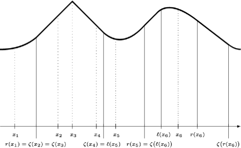
Figure 1: Illustration of the functions $\zeta$, $\ell$, $r$ appearing in the proof of Lemma 1. The vertical solid lines also demarcate the region ${\mathcal{C}}$.

Given a function $u$ that satisfies the requirements of Definition 1, we now use the notation and the terminology introduced by Definitions 1 and 2 to iteratively construct a process $\xi^{*}\in{\mathcal{A}}_{\mathrm{c}}$ such that (1)–(1) hold true by means of the constructions above. To this end, we introduce the following notation, which is illustrated by Figure 1. If $\operatorname{int}{\mathcal{C}}\neq\varnothing$ and $x\in{\mathcal{C}}$, then we recall that we use $u_{-}^{\prime}(x)$ [resp., $u_{+}^{\prime}(x)$] to denote the left-hand (resp., the right-hand) first derivative of $u$ at $x$, we define

$$\zeta(x)=\cases{\displaystyle\sup\{y<x\mid y\notin{\mathcal{C}}\},&\quad if $u_{-}^{\prime}(x)=1$,\cr\displaystyle\inf\{y>x\mid y\notin{\mathcal{C}}\},&\quad if $u_{+}^{\prime}(x)=-1$ and $u_{-}^{\prime}(x)<1$,}$$

and we note that $\zeta(x)\in{\mathbb{R}}$ because $u$ is real-valued. On the other hand, given any $x\in{\mathbb{R}}$, we define

$$\ell(x)=\sup\{y<x\mid y\in\operatorname{int}{\mathcal{C}}\}\quad\mbox{and}\quad r(x)=\inf\{y>x\mid y\in\operatorname{int}{\mathcal{C}}\},$$

with the usual conventions that $\sup\varnothing=-\infty$ and $\inf\varnothing=\infty$. The algorithm that we now develop terminates after finite iterations because each of the sets ${\mathcal{C}}$, ${\mathcal{W}}$ is a finite union of intervals.

STEP 0: Initialization. We consider the following four possibilities that can happen, depending on the initial condition $x$ of (1):

If $\operatorname{int}{\mathcal{C}}\neq\varnothing$ and $x\in\operatorname{int}{\mathcal{C}}$ (e.g., see the points $x_{2}$, $x_{3}$, $x_{4}$ in Figure 1), then we define $\xi_{t}^{0}=\zeta(x)-x$ for all $t>0$. If we denote by $X^{0}$ the corresponding solution to (1), and we set $\tau_{0}=0$, then $X^{0}$ has a single jump at time $\tau_{0}$,

In this case, $X_{0}\in{\mathcal{B}}$ if $x\in{\mathcal{B}}\subseteq{\mathcal{C}}$.

If $\ell(x)=-\infty$ and $r(x)=\infty$, which is the case if $\operatorname{int}{\mathcal{C}}=\varnothing$, then we define $\xi^{0}=0$, we denote by $X^{0}$ the corresponding solution to (1), and we let $\tau_{0}=\infty$.

If $\operatorname{int}{\mathcal{C}}\neq\varnothing$, $x\in{\mathbb{R}}\setminus\operatorname{int}{\mathcal{C}}$ and either of $\ell(x)$, $r(x)$ is reflecting (e.g., see the points $x_{1}$, $x_{5}$ in Figure 1), then we define $\xi^{0}=0$, we denote by $X^{0}$ the corresponding solution to (1), and we set $\tau_{0}=0$.

If $\operatorname{int}{\mathcal{C}}\neq\varnothing$, $x\in{\mathbb{R}}\setminus\operatorname{int}{\mathcal{C}}$, and both $\ell(x)$, $r(x)$ are repelling if finite (e.g., see the point $x_{6}$ in Figure 1), then we consider the $({\mathcal{F}}_{t})$-stopping times

$$T_{\ell(x)}=\inf\bigl{\{}t\geq 0\mid X_{t}^{\dagger}\leq\ell(x)\bigr{\}},\qquad T_{r(x)}=\inf\bigl{\{}t\geq 0\mid X_{t}^{\dagger}\geq r(x)\bigr{\}},$$

where $X^{\dagger}$ is the solution to (1) for $\xi=0$, and we set

$$\xi_{t}^{0}=\bigl{[}\zeta\bigl{(}\ell(x)\bigr{)}-\ell(x)\bigr{]}\mathbf{1}_{\{T_{\ell(x)}<T_{r(x)}\wedge t\}}+\bigl{[}\zeta\bigl{(}r(x)\bigr{)}-r(x)\bigr{]}\mathbf{1}_{\{T_{r(x)}<T_{\ell(x)}\wedge t\}},$$

in which expression, we define $\zeta(\ell(x))-\ell(x)$ [resp., $\zeta(r(x))-r(x)$] arbitrarily if $\ell(x)=-\infty$ [resp., $r(x)=\infty$]. If we denote by $X^{0}$ the corresponding solution to (1), and we set $\tau_{0}=T_{r(x)}\wedge T_{\ell(x)}$, then $X^{0}$ has a single jump at the $({\mathcal{F}}_{t})$-stopping time $\tau_{0}$,

$$\displaystyle X_{t}^{0}\in{\mathbb{R}}\setminus\operatorname{int}{\mathcal{C}}\quad\mbox{and}\quad u\bigl{(}X_{t+}^{0}\bigr{)}-u\bigl{(}X_{t}^{0}\bigr{)}=-\bigl{|}\Delta\xi_{t}^{0}\bigr{|}\qquad\mbox{for all }t\leq\tau_{0},$$

In this case, we may have $X_{\tau_{0}}^{0}\in{\mathcal{B}}$ but $X_{\tau_{0}+}^{0}\notin{\mathcal{B}}$ and $X_{t}^{0}\notin{\mathcal{B}}$ for all $t<\tau_{0}$.

STEP 1: Induction hypothesis. We assume that we have determined an $({\mathcal{F}}_{t})$-stopping time $\tau_{j}$, and we have constructed a process $\xi^{j}\in{\mathcal{A}}_{\mathrm{c}}$ such that, if we denote by $X^{j}$ the associated solution to (1), then (1)–(1) are satisfied for $\xi^{j}$, $X^{j}$ in place of $\xi^{*}$, $X^{*}$ and for all $t\leq\tau_{j}$ instead of all positive $t$. Also, we assume that, if ${\mathbb{P}}(\tau_{j}<\infty)>0$, then one of the following two possibilities occur: [(II)]

there exists a point $x^{j}$ such that $X_{\tau_{j}}^{j}=x^{j}$ on the event $\{\tau_{j}<\infty\}$;

there exist points $x_{1}^{j}$, $x_{2}^{j}\in{\mathbb{R}}$ and events $A_{1}^{j},A_{2}^{j}\in{\mathcal{F}}_{\tau_{j}}$ forming a partition of $\{\tau_{j}<\infty\}$ such that ${\mathbb{P}}(A_{k}^{j})>0$, $X_{\tau_{j}+}^{j}=x_{k}^{j}$ on the event $A_{k}^{j}$ and at least one of $\ell(x_{k}^{j})$, $r(x_{k}^{j})$ is finite and reflecting, for $k=1,2$.

Step 0 provides such a construction for $j=0$. In particular, the last possibility there gives rise to Case (II) for

$$A_{1}^{0} = \{T_{\ell(x)}<T_{r(x)}\},\qquad A_{2}^{0}=\{T_{r(x)}<T_{\ell(x)}\},$$

$$x_{1}^{0} = \zeta\bigl{(}\ell(x)\bigr{)}\quad\mbox{and}\quad x_{2}^{0}=\zeta\bigl{(}r(x)\bigr{)}.$$

On the other hand, the second possibility there is such that ${\mathbb{P}}(\tau_{j}<\infty)=0$, while the remaining two possibilities give rise to Case (I).

STEP 2. If ${\mathbb{P}}(\tau_{j}<\infty)=0$, then define $\xi^{*}=\xi^{j}$, $X^{*}=X^{j}$ and stop. Otherwise, we proceed to the next step.

STEP 3. We address the situation arising in the context of Case (II) of Step 1; the analysis regarding Case (I) is simpler and follows exactly the same steps. To this end, we first consider the $({\mathcal{F}}_{t})$-stopping time $\hat{\tau}=\tau_{j}\mathbf{1}_{A_{1}^{j}}+\infty\mathbf{1}_{A_{2}^{j}}$, and we note that $X_{\hat{\tau}}^{j}=x_{1}^{j}$ on the event $\{\hat{\tau}<\infty\}$. We are faced with the following possible cases.

If both of $\ell(x_{1}^{j})$, $r(x_{1}^{j})$ are finite and reflecting, then we appeal to the construction associated with (22)–(4) for $\xi=\xi^{j}$, $X=X^{j}$, $\bar{x}=x_{1}^{j}$ and $\tau=\hat{\tau}$ to obtain processes $\tilde{\xi}$, $\tilde{X}$ that are equal to $\xi^{j}$, $X^{j}$ up to time $\hat{\tau}$ and satisfy (4) for all $t>\hat{\tau}$. We then define

$$\xi^{j+1}=\tilde{\xi},\qquad X^{j+1}=\tilde{X}\quad\mbox{and}\quad\tau_{j+1}=\infty\mathbf{1}_{A_{1}^{j}}+\tau_{j}\mathbf{1}_{A_{2}^{j}}.$$

The result of this construction is such that $X_{\tau_{j+1}+}^{j+1}=x_{2}^{j}$ on the event $\{\tau_{j+1}<\infty\}=A_{2}^{j}$, which puts us in the context of Case (I) of Step 1.

If $\ell(x_{1}^{j})$ is finite and reflecting and $r(x_{1}^{j})=\infty$ [resp., $\ell(x_{1}^{j})=-\infty$ and $r(x_{1}^{j})$ is finite and reflecting], then we proceed in the same way using the construction associated with (24)–(25) [resp., (27)–(28)].

If $\ell(x_{1}^{j})$ is finite and reflecting and $r(x_{1}^{j})$ is finite and repelling, then we consider (24)–(25) and, as above, we construct processes $\tilde{\xi}$, $\tilde{X}$ that are equal to $\xi^{j}$, $X^{j}$ up to time $\hat{\tau}$ and satisfy (25) for all $t>\hat{\tau}$. We then consider the $({\mathcal{F}}_{t})$-stopping time $\hat{\tau}^{\dagger}$ and the process $\xi^{j+1}\in{\mathcal{A}}_{\mathrm{c}}$ given by

$$\hat{\tau}^{\dagger} = \inf\bigl{\{}t\geq\hat{\tau}\mid\tilde{X}_{t}\geq r\bigl{(}x_{1}^{j}\bigr{)}\bigr{\}}\quad\mbox{and}$$

$$\xi_{t}^{j+1} = \cases{\displaystyle\tilde{\xi}_{t},&\quad if $t\leq\hat{\tau}^{\dagger}$,\cr\displaystyle\tilde{\xi}_{\hat{\tau}^{\dagger}}+\zeta\bigl{(}r\bigl{(}x_{1}^{j}\bigr{)}\bigr{)}-r\bigl{(}x_{1}^{j}\bigr{)},&\quad if $t>\hat{\tau}^{\dagger}$,}$$

we denote by $X^{j+1}$ the associated solution to (1), and we define

$$\tau_{j+1} = \hat{\tau}^{\dagger}\mathbf{1}_{A_{1}^{j}}+\tau_{j}\mathbf{1}_{A_{2}^{j}},\qquad A_{1}^{j+1}=\bigl{\{}\hat{\tau}^{\dagger}<\infty\bigr{\}},\qquad A_{2}^{j+1}=A_{2}^{j},$$

$$x_{i}^{j+1} = \zeta\bigl{(}r\bigl{(}x_{1}^{j}\bigr{)}\bigr{)}\quad\mbox{and}\quad x_{2}^{j+1}=x_{2}^{j}.$$

In this case, we may have $X_{\tau_{j+1}}\in{\mathcal{B}}$ but $X_{\tau_{j+1}+}\notin{\mathcal{B}}$ and $X_{t}\notin{\mathcal{B}}$ for all $t\in\,]\tau_{j},\tau_{j+1}[$.

Finally, if $\ell(x_{1}^{j})$ is finite and repelling, and $r(x_{1}^{j})$ is finite and reflecting, then we are faced with a construction that is symmetric to the very last one using (27)–(28).

STEP 4. Go back to Step 2.

We now prove the main result of the section. It is worth noting that we can relax significantly assumptions (34)–(35). However, we have opted against any such relaxation because (a) this would require a considerable amount of extra arguments of a technical nature that would obscure the main ideas of the proof, and (b) (34)–(35) are plainly satisfied in the special cases that we explicitly solve in Sections 5 and 6.

Theorem 1

Consider a function $u\dvtx{\mathbb{R}}\rightarrow{\mathbb{R}}_{+}$ that satisfies the conditions of Definition 1, let $\xi^{*}\in{\mathcal{A}}_{\mathrm{c}}$ be the control strategy constructed in Lemma 1, let $X^{*}$ be the associated solution to (1) and define

$$v(y)=\max\bigl{\{}u(y),g(y)\bigr{\}}\quad\mbox{and}\quad w(y)=u(y)\qquad\mbox{for }y\in{\mathbb{R}}.$$ (32)

Also, given any $\xi\in{\mathcal{A}}_{\mathrm{c}}$, define

$$\tau_{v}^{*} = \tau_{v}^{*}(\xi)=\inf\{t\geq 0\mid X_{t}\in{\mathcal{S}}\},$$

$$\tau_{w}^{*} = \tau_{w}^{*}(\xi)=\inf\{t\geq 0\mid X_{t+}\in{\mathcal{S}}\},$$

where $X$ is the associated solution to (1), and note that $\tau_{v}^{*}\vee\tau_{w}^{*}=\tau_{w}^{*}$. In this context, the following statements are true: [(III)]

$J_{x}^{v}(\xi^{*},\tau)\leq v(x)$ and $J_{x}^{w}(\xi^{*},\tau)\leq w(x)$ for all $\tau\in{\mathcal{A}}_{\mathrm{s}}$ and all initial conditions of (1).

$v(x)=J_{x}^{v}(\xi^{*},\tau_{v}^{*})$ and $w(x)=J_{x}^{w}(\xi^{*},\tau_{w}^{*})$ for every initial condition $x$ of (1) such that

$$\sup_{t\geq 0}u\bigl{(}X_{t}^{*}\bigr{)}\leq K_{1}$$ (34)

for some constant $K_{1}=K_{1}(x)$.

If there exists a constant $K_{2}$ such that

$$u(y)\leq K_{2}\qquad\mbox{for all }y\in{\mathbb{R}}\setminus{\mathcal{S}},$$ (35)

then $v(x)\leq J_{x}^{v}(\xi,\tau_{v}^{*})$ and $w(x)\leq J_{x}^{w}(\xi,\tau_{w}^{*})$ for every initial condition $x$ of (1).

If $u$ satisfies (35), then $(\xi^{*},\tau_{v}^{*})$ [resp., $(\xi^{*},\tau_{w}^{*})$] is an optimal strategy for the game with performance criterion given by (2) [resp., (3)] and $v$ and $w$ are the value functions of the two games.

Given a function $u$ satisfying the conditions of Definition 1, we denote by $u^{\prime\prime}$ the unique, Lebesgue-a.e., first derivative of $u^{\prime}$ in ${\mathbb{R}}\setminus{\mathcal{B}}$, and we define $u^{\prime\prime}(x)$, $u^{\prime}(x)$ arbitrarily for $x$ in the finite set ${\mathcal{B}}$. In view of (1), we can use Itô’s formula and the integration by parts formula to calculate

$$e^{-\Lambda_{T}}u\bigl{(}X_{T}^{*}\bigr{)} = u(x)+\int_{0}^{T}e^{-\Lambda_{t}}{\mathcal{L}}u\bigl{(}X_{t}^{*}\bigr{)}\,dt+\int_{[0,T[}e^{-\Lambda_{t}}u^{\prime}\bigl{(}X_{t}^{*}\bigr{)}\,d\xi_{t}$$

$${}+\sum_{0\leq t<T}e^{-\Lambda_{t}}\bigl{[}u\bigl{(}X_{t+}^{*}\bigr{)}-u\bigl{(}X_{t}^{*}\bigr{)}-u^{\prime}\bigl{(}X_{t}^{*}\bigr{)}\Delta X_{t}^{*}\bigr{]}+M_{T}^{*},$$

where

$$M_{T}^{*}=\int_{0}^{T}e^{-\Lambda_{t}}\sigma\bigl{(}X_{t}^{*}\bigr{)}u^{\prime}\bigl{(}X_{t}^{*}\bigr{)}\,dW_{t}.$$ (36)

Rearranging terms and using (1)–(1), we obtain

$$\int_{0}^{T}e^{-\Lambda_{t}}h\bigl{(}X_{t}^{*}\bigr{)}\,dt+\int_{[0,T[}e^{-\Lambda_{t}}\,d\check{\xi}_{t}^{*}+e^{-\Lambda_{T}}u\bigl{(}X_{T}^{*}\bigr{)}$$

$$\qquad=u(x)+\int_{0}^{T}e^{-\Lambda_{t}}\bigl{[}{\mathcal{L}}u\bigl{(}X_{t}^{*}\bigr{)}+h\bigl{(}X_{t}^{*}\bigr{)}\bigr{]}\,dt+\int_{0}^{T}e^{-\Lambda_{t}}\bigl{[}1+u^{\prime}\bigl{(}X_{t}^{*}\bigr{)}\bigr{]}\,d\bigl{(}\xi^{*{\mathrm{c}}}\bigr{)}_{t}^{+}$$

$$\qquad\quad{}+\int_{0}^{T}e^{-\Lambda_{t}}\bigl{[}1-u^{\prime}\bigl{(}X_{t}^{*}\bigr{)}\bigr{]}\,d\bigl{(}\xi^{*{\mathrm{c}}}\bigr{)}_{t}^{-}$$

$$\qquad\quad{}+\sum_{0\leq t<T}e^{-\Lambda_{t}}\bigl{[}u\bigl{(}X_{t+}^{*}\bigr{)}-u\bigl{(}X_{t}^{*}\bigr{)}+\bigl{|}\Delta X_{t}^{*}\bigr{|}\bigr{]}+M_{T}^{*}$$

$$\qquad=u(x)+\int_{0}^{T}e^{-\Lambda_{t}}\bigl{[}{\mathcal{L}}u\bigl{(}X_{t}^{*}\bigr{)}+h\bigl{(}X_{t}^{*}\bigr{)}\bigr{]}\,dt+M_{T}^{*}.$$

It follows that, given any finite $({\mathcal{F}}_{t})$-stopping time $\hat{\tau}$,

$$\int_{0}^{\hat{\tau}}e^{-\Lambda_{t}}h\bigl{(}X_{t}^{*}\bigr{)}\,dt+\int_{[0,\hat{\tau}[}e^{-\Lambda_{t}}\,d\check{\xi}_{t}^{*}+e^{-\Lambda_{\hat{\tau}}}g\bigl{(}X_{\hat{\tau}}^{*}\bigr{)}$$

$$\qquad=u(x)+e^{-\Lambda_{\hat{\tau}}}\bigl{[}g\bigl{(}X_{\hat{\tau}}^{*}\bigr{)}-u\bigl{(}X_{\hat{\tau}}^{*}\bigr{)}\bigr{]}+\int_{0}^{\hat{\tau}}e^{-\Lambda_{t}}\bigl{[}{\mathcal{L}}u\bigl{(}X_{t}^{*}\bigr{)}+h\bigl{(}X_{t}^{*}\bigr{)}\bigr{]}\,dt+M_{\hat{\tau}}^{*}$$

(37)

$$\qquad=u(x)\mathbf{1}_{\{0<\hat{\tau}\}}+e^{-\Lambda_{\hat{\tau}}}\bigl{[}g\bigl{(}X_{\hat{\tau}}^{*}\bigr{)}-u\bigl{(}X_{\hat{\tau}}^{*}\bigr{)}\bigr{]}\mathbf{1}_{\{0<\hat{\tau}\}}+g(x)\mathbf{1}_{\{\hat{\tau}=0\}}$$

$$\qquad\quad{}+\int_{0}^{\hat{\tau}}e^{-\Lambda_{t}}\bigl{[}{\mathcal{L}}u\bigl{(}X_{t}^{*}\bigr{)}+h\bigl{(}X_{t}^{*}\bigr{)}\bigr{]}\,dt+M_{\hat{\tau}}^{*}.$$

Similarly, we can calculate

$$\int_{0}^{\hat{\tau}}e^{-\Lambda_{t}}h\bigl{(}X_{t}^{*}\bigr{)}\,dt+\int_{[0,\hat{\tau}]}e^{-\Lambda_{t}}\,d\check{\xi}_{t}^{*}+e^{-\Lambda_{\hat{\tau}}}g\bigl{(}X_{\hat{\tau}+}^{*}\bigr{)}$$

$$\qquad=u(x)+e^{-\Lambda_{\hat{\tau}}}\bigl{[}g\bigl{(}X_{\hat{\tau}+}^{*}\bigr{)}-u\bigl{(}X_{\hat{\tau}+}^{*}\bigr{)}\bigr{]}$$ (38)

$$\qquad\quad{}+\int_{0}^{\hat{\tau}}e^{-\Lambda_{t}}\bigl{[}{\mathcal{L}}u\bigl{(}X_{t}^{*}\bigr{)}+h\bigl{(}X_{t}^{*}\bigr{)}\bigr{]}\,dt+M_{\hat{\tau}}^{*}.$$

Combining (4) with (1) and the facts that $0\leq g(x)\leq u(x)$ for all $x\in{\mathbb{R}}\setminus{\mathcal{C}}=\operatorname{int}({\mathcal{W}}\cup{\mathcal{S}}_{\mathcal{W}})$ and ${\mathcal{L}}u(x)+h(x)\leq 0$ Lebesgue-a.e. in ${\mathbb{R}}\setminus{\mathcal{C}}$, we can see that, given any $T>0$ and any $({\mathcal{F}}_{t})$-stopping time $\tau$,

$$\int_{0}^{T\wedge\tau}e^{-\Lambda_{t}}h\bigl{(}X_{t}^{*}\bigr{)}\,dt+\int_{[0,T\wedge\tau[}e^{-\Lambda_{t}}\,d\check{\xi}_{t}^{*}+e^{-\Lambda_{\tau}}g\bigl{(}X_{\tau}^{*}\bigr{)}\mathbf{1}_{\{\tau\leq T\}}$$

(39)

$$\qquad\leq u(x)\mathbf{1}_{\{0<\tau\}}+g(x)\mathbf{1}_{\{\tau=0\}}+M_{T\wedge\tau}^{*}\leq v(x)+M_{T\wedge\tau}^{*},$$

the last inequality following thanks to (32). These inequalities and the positivity of $h$, $g$ imply that the stopped process $M^{*\tau}$ is a supermartingale and ${\mathbb{E}}[M_{T\wedge\tau}^{*}]\leq 0$. Therefore, we can take expectations in (4) and pass to the limit $T\rightarrow\infty$ using Fatou’s lemma to obtain the inequality $J_{x}^{v}(\xi^{*},\tau)\leq\max\{u(x),g(x)\}=v(x)$. With reasoning similar to (4), we derive the inequality $J_{x}^{w}(\xi^{*},\tau)\leq u(x)=w(x)$, and (I) follows.

To prove (II), we consider the $({\mathcal{F}}_{t})$-stopping time $\tau_{v}^{*}$ defined by (1) with $X^{*}$ instead of $X$, and we note that

$$X_{t}^{*}\in\operatorname{cl}{\mathcal{W}}={\mathbb{R}}\setminus\operatorname{int}({\mathcal{C}}\cup{\mathcal{S}})\qquad\mbox{for all }0<t\leq\tau_{v}^{*}.$$

Combining this observation and the definition of $\tau_{v}^{*}$ with the facts that $g(x)\leq u(x)=v(x)$ for all $x\in{\mathcal{W}}$ and $v(x)=g(x)$ for all $x\in{\mathcal{S}}$, we can see that

$$u\bigl{(}X_{\tau_{v}^{*}}^{*}\bigr{)}\mathbf{1}_{\{\tau_{v}^{*}>0\}} = g\bigl{(}X_{\tau_{v}^{*}}^{*}\bigr{)}\mathbf{1}_{\{\tau_{v}^{*}>0\}},$$

$$v(x)\mathbf{1}_{\{\tau_{v}^{*}=0\}} = g(x)\mathbf{1}_{\{\tau_{v}^{*}=0\}}\quad\mbox{and}\quad v(x)\mathbf{1}_{\{\tau_{v}^{*}>0\}}=u(x)\mathbf{1}_{\{\tau_{v}^{*}>0\}}.$$

In view of these observations, (4) and the fact that ${\mathcal{L}}u(x)+h(x)=0$ Lebesgue-a.e. in ${\mathcal{W}}$, we can see that, given any $T>0$,

$$\int_{0}^{T\wedge\tau_{v}^{*}}e^{-\Lambda_{t}}h\bigl{(}X_{t}^{*}\bigr{)}\,dt+\int_{[0,T\wedge\tau_{v}^{*}[}e^{-\Lambda_{t}}\,d\check{\xi}_{t}^{*}+e^{-\Lambda_{\tau_{v}^{*}}}g\bigl{(}X_{\tau_{v}^{*}}^{*}\bigr{)}\mathbf{1}_{\{\tau_{v}^{*}\leq T\}}$$

$$\quad{}+e^{-\Lambda_{T}}u\bigl{(}X_{T}^{*}\bigr{)}\mathbf{1}_{\{T<\tau_{v}^{*}\}}$$

$$\qquad=u(x)\mathbf{1}_{\{0<\tau_{v}^{*}\}}+e^{-\Lambda_{\tau_{v}^{*}}}\bigl{[}g\bigl{(}X_{\tau_{v}^{*}}^{*}\bigr{)}-u\bigl{(}X_{\tau_{v}^{*}}^{*}\bigr{)}\bigr{]}\mathbf{1}_{\{0<\tau_{v}^{*}\leq T\}}+g(x)\mathbf{1}_{\{\tau_{v}^{*}=0\}}$$

$$\qquad\quad{}+M_{T\wedge\tau_{v}^{*}}^{*}$$

$$\qquad=v(x)+M_{T\wedge\tau_{v}^{*}}^{*}.$$

If we denote by $(\varrho_{n})$ a localizing sequence for the stopped local martingale $M^{*\tau_{v}^{*}}$ such that $\varrho_{n}>0$ for all $n\geq 1$, then we can see that these identities imply that

$${\mathbb{E}}\biggl{[}\int_{0}^{\varrho_{n}\wedge\tau_{v}^{*}}e^{-\Lambda_{t}}h\bigl{(}X_{t}^{*}\bigr{)}\,dt+\int_{[0,\varrho_{n}\wedge\tau_{v}^{*}[}e^{-\Lambda_{t}}\,d\check{\xi}_{t}^{*}+e^{-\Lambda_{\tau_{v}^{*}}}g\bigl{(}X_{\tau_{v}^{*}}^{*}\bigr{)}\mathbf{1}_{\{\tau_{v}^{*}\leq\varrho_{n}\}}$$

$$\hskip 185.0pt\qquad{}+e^{-\Lambda_{\varrho_{n}}}u\bigl{(}X_{\varrho_{n}}^{*}\bigr{)}\mathbf{1}_{\{\varrho_{n}<\tau^{*}\}}\biggr{]}=v(x).$$

In view of (34) and Assumption 2, we can pass to the limit as $n\rightarrow\infty$ using the monotone and the dominated convergence theorems to obtain $J_{x}^{v}(\xi^{*},\tau^{*})=\max\{u(x),g(x)\}=v(x)$.

We can use (4) and the observations that

$$X_{t}^{*}\in\operatorname{cl}{\mathcal{W}}={\mathbb{R}}\setminus\operatorname{int}({\mathcal{C}}\cup{\mathcal{S}})\qquad\mbox{for all }0<t\leq\tau_{w}^{*}\quad\mbox{and}\quad u\bigl{(}X_{\tau_{w}^{*}+}^{*}\bigr{)}=g\bigl{(}X_{\tau_{w}^{*}+}^{*}\bigr{)}$$

to show that $J_{x}^{w}(\xi^{*},\tau^{*})=u(x)=w(x)$ similarly.

To establish Part (III), we consider any admissible $\xi\in{\mathcal{A}}_{\mathrm{c}}$ and we note that (4) remains true with $\xi$, $X$ instead of $\xi^{*}$, $X^{*}$ if $\hat{\tau}$ is replaced by $\hat{\tau}\wedge\tau_{v}^{*}$ because ${\mathcal{B}}\subseteq{\mathcal{S}}$. Also, we note that

$$X_{t}\in{\mathbb{R}}\setminus{\mathcal{S}}=({\mathcal{W}}\cup{\mathcal{C}})\setminus{\mathcal{S}}\qquad\mbox{for all }t<\tau_{v}^{*}.$$ (40)

In view of the facts that $g(x)\leq u(x)=v(x)$ for all $x\in{\mathbb{R}}\setminus{\mathcal{S}}$ and $u(x)\leq g(x)=v(x)$ for all $x\in{\mathcal{S}}$, we can see that this observation and the definition of $\tau_{v}^{*}$ imply that

$$u(X_{\tau_{v}^{*}})\mathbf{1}_{\{\tau_{v}^{*}>0\}} \leq g(X_{\tau_{v}^{*}})\mathbf{1}_{\{\tau_{v}^{*}>0\}},$$

$$v(x)\mathbf{1}_{\{\tau_{v}^{*}=0\}} = g(x)\mathbf{1}_{\{\tau_{v}^{*}=0\}}\quad\mbox{and}\quad v(x)\mathbf{1}_{\{\tau_{v}^{*}>0\}}=u(x)\mathbf{1}_{\{\tau_{v}^{*}>0\}}.$$

Combining these observations with the fact that ${\mathcal{L}}u(x)+h(x)\geq 0$ Lebesgue-a.e. inside $\operatorname{int}[({\mathcal{W}}\cup{\mathcal{C}})\setminus{\mathcal{S}}]$, we can see that (4) implies that, given any $T>0$,

$$\int_{0}^{T\wedge\tau_{v}^{*}}e^{-\Lambda_{t}}h(X_{t})\,dt+\int_{[0,T\wedge\tau_{v}^{*}[}e^{-\Lambda_{t}}\,d\check{\xi}_{t}+e^{-\Lambda_{\tau_{v}^{*}}}g(X_{\tau_{v}^{*}})\mathbf{1}_{\{\tau_{v}^{*}\leq T\}}$$

$$\quad{}+e^{-\Lambda_{T}}u(X_{T})\mathbf{1}_{\{T<\tau_{v}^{*}\}}$$

$$\qquad\geq u(x)\mathbf{1}_{\{0<\tau_{v}^{*}\}}+e^{-\Lambda_{\tau_{v}^{*}}}\bigl{[}g(X_{\tau_{v}^{*}})-u(X_{\tau_{v}^{*}})\bigr{]}\mathbf{1}_{\{0<\tau_{v}^{*}\leq T\}}+g(x)\mathbf{1}_{\{\tau_{v}^{*}=0\}}$$

$$\qquad\quad{}+M_{T\wedge\tau_{v}^{*}}$$

$$\qquad\geq v(x)+M_{T\wedge\tau_{v}^{*}},$$

where $M$ is defined as in (36). If $(\varrho_{n})$ is a localizing sequence for the stopped local martingale $M^{\tau_{v}^{*}}$ such that $\varrho_{n}>0$ for all $n\geq 1$, then these inequalities imply that

$${\mathbb{E}}\biggl{[}\int_{0}^{\varrho_{n}\wedge\tau_{v}^{*}}e^{-\Lambda_{t}}h(X_{t})\,dt+\int_{[0,\varrho_{n}\wedge\tau_{v}^{*}[}e^{-\Lambda_{t}}\,d\check{\xi}_{t}+e^{-\Lambda_{\tau_{v}^{*}}}g(X_{\tau_{v}^{*}})\mathbf{1}_{\{\tau_{v}^{*}\leq\varrho_{n}\}}$$

$$\hskip 181.0pt\qquad{}+e^{-\Lambda_{\varrho_{n}}}u\bigl{(}X_{\varrho_{n}}^{*}\bigr{)}\mathbf{1}_{\{\varrho_{n}<\tau^{*}\}}\biggr{]}\geq v(x).$$

In view of (35) and Assumption 2, we can pass to the limit as $n\rightarrow\infty$ using the monotone and the dominated convergence theorems to obtain $J_{x}^{v}(\xi,\tau^{*})\geq\max\{u(x),g(x)\}=v(x)$.

In general, the inequality $\tau_{v}^{*}\leq\tau_{w}^{*}$ may be strict because, for example, we may have $x\in{\mathcal{S}}$ and $x+\Delta\xi_{0}\in{\mathbb{R}}\setminus{\mathcal{S}}$. In such a case, the set $\{t\in[0,\tau_{w}^{*}[\,\mid X_{t}\in{\mathcal{B}}\}$ may not be empty, but it is finite. Therefore, we can use Itô’s formula to derive (4) with $\xi$, $X$ instead of $\xi^{*}$, $X^{*}$ and with $\hat{\tau}\wedge\tau_{v}^{*}$ replacing $\hat{\tau}$. Combining this result with the observations that

$$X_{t}\in\operatorname{cl}({\mathbb{R}}\setminus{\mathcal{S}})\qquad\mbox{for all }0<t<\tau_{w}^{*}\quad\mbox{and}\quad u(X_{\tau_{w}^{*}+})\leq g(X_{\tau_{w}^{*}+}),$$

we can derive the inequality $J_{x}^{w}(\xi,\tau^{*})\geq u(x)=w(x)$ as above.

Finally, Part (IV) follows immediately from Parts (I)–(III).

Remark 1.

An inspection of the proof of Theorem 1 reveals that the optimal strategy $(\xi^{*},\tau_{w}^{*})$ of the game where the controller has the first-move advantage is highly nonunique. Indeed, in the presence of (35), $(\xi^{*},\tilde{\tau}_{w}^{*})$, where $\tilde{\tau}_{w}^{*}$ is any $({\mathcal{F}}_{t})$-stopping time such that $X_{\tilde{\tau}_{w}^{*}+}^{*}\mathbf{1}_{\{\tilde{\tau}_{w}^{*}<\infty\}}\in{\mathcal{S}}$, in particular, $(\xi^{*},\infty)$, is also an optimal strategy. It is worth noting that a similar observation cannot be made for the game where the stopper has the first-move advantage. Both of the special cases considered in the following two sections provide cases illustrating this situation; see Propositions 4, 5, 7 and 8.

5 The explicit solution to a special case with quadratic reward functions

We now derive the explicit solution to the special case of the general problem that arises when

$$b(x) = 0,\qquad\sigma(x)=1,\qquad\bar{\delta}(x)=\delta,\qquad h(x)=\kappa x^{2}+\mu\quad\mbox{and}$$

$$g(x) = \lambda x^{2}\qquad\mbox{for all }x\in{\mathbb{R}},$$

for some constants $\delta,\kappa,\lambda>0$ and $\mu\geq 0$. In our analysis, we exploit the symmetry around the origin that the problem has, we consider only sets $\Gamma\subseteq{\mathbb{R}}$ such that $\{-x\mid x\in\Gamma\}=\Gamma$ and we denote $\Gamma^{+}=\Gamma\cap[0,\infty[$. Also, we recall that the general solution to the ODE

$${\mathcal{L}}f(x)+h(x)\equiv{\tfrac{1}{2}}f^{\prime\prime}(x)-\delta f(x)+\kappa x^{2}+\mu=0$$

is given by

$$f(x)=A\cosh\sqrt{2\delta}x+B\sinh\sqrt{2\delta}x+\frac{\kappa}{\delta}x^{2}+\frac{\kappa+\delta\mu}{\delta^{2}}$$

for some constants $A,B\in{\mathbb{R}}$.

In the special case that we consider in this section, the controller should exert effort to keep the state process close to the origin. On the other hand, the stopper should terminate the game if the state process is sufficiently far from the origin. In view of these observations, we derive optimal strategies by considering functions satisfying the requirements of Definition 1 that are associated with the regions

$${\mathcal{S}}^{+}=[\alpha,\infty[,\qquad{\mathcal{C}}^{+}=[\beta,\infty[\quad\mbox{and}\quad{\mathcal{W}}^{+}=[0,\alpha\wedge\beta[$$ (41)

for some constants $\alpha,\beta>0$; see Definition 1. In particular, we derive three qualitatively different cases that are characterized by the relations $\beta<\alpha$, $\alpha<\beta$ or $\alpha=\beta$, depending on parameter values; see Figures 2–4 as well as Remark 2.

In this context, Theorem 1 implies that the associated optimal strategies can be described informally as follows. The controlled process $\xi^{*}$ has an initial jump equal to $-(x+\beta)$ [resp., $-(x-\beta)$] if the initial condition $x$ of (1) is such that $x<-\beta$ (resp., $x>\beta$). Beyond time 0, $\xi^{*}$ is such that the associated solution to (1) is reflecting in $-\beta$ in the positive direction and in $\beta$ in the negative direction. On the other hand, the optimal stopping times $\tau_{v}^{*}$, $\tau_{w}^{*}$ are the first hitting times of ${\mathcal{S}}$ as defined by (1). In view of these observations, we focus on the construction of the function $u$ satisfying the requirements of Definition 1 in what follows.

Figure 2: The functions $v$ and $w$ in the context of Proposition 2 ($\beta<\alpha$).

In the first case that we consider, $u$ identifies with the value function of the singular stochastic control problem that arises if the stopper never terminates the game (see Figure 2). In particular, we look for a solution to the variational inequality

$$\min\bigl{\{}{\tfrac{1}{2}}u^{\prime\prime}(x)-\delta u(x)+\kappa x^{2}+\mu,1-\bigl{|}u^{\prime}(x)\bigr{|}\bigr{\}}=0$$ (42)

of the form

$$u(x)=\cases{\displaystyle A\cosh\sqrt{2\delta}x+\frac{\kappa}{\delta}x^{2}+\frac{\kappa+\delta\mu}{\delta^{2}},&\quad if $|x|\leq\beta$,\cr\displaystyle x-\beta+u(\beta),&\quad if $|x|>\beta$.}$$ (43)

The requirement that $u$ should be $C^{2}$ along the free-boundary point $\beta$, which is associated with the so-called “principle of smooth fit” of singular stochastic control, implies that the parameter $A$ should be given by

$$A=-\frac{\kappa}{\delta^{2}\cosh\sqrt{2\delta}\beta},$$ (44)

while $\beta>0$ should satisfy

$$\tanh\sqrt{2\delta}\beta=\frac{\delta(2\kappa\beta-\delta)}{\kappa\sqrt{2\delta}}.$$ (45)

We also define $\alpha>0$ to be the unique solution to the equation

$$u(\alpha)=\lambda\alpha^{2}.$$ (46)

We prove the following result, as well as the other ones we consider in this section, in Appendix I.

Proposition 2

Equation (45) has a unique solution $\beta>0$, which is strictly greater than $\frac{\delta}{2\kappa}$, while equation (46) has a unique solution $\alpha>0$. Furthermore, $\alpha>\beta$ if and only if

$$\quad\delta\lambda-\kappa<0\hskip 5.0pt \mbox{or}\quad\delta\lambda-\kappa=0\quad\mbox{and}\quad\mu>0$$

$$\mbox{or}\quad\delta\lambda-\kappa>0\quad\mbox{and}\quad\tanh\sqrt{\frac{2\delta\mu}{\delta\lambda-\kappa}}<\sqrt{\frac{2\delta\mu}{\delta\lambda-\kappa}}-\frac{\delta^{2}}{\kappa\sqrt{2\delta}},$$

in which case, $\alpha>\frac{1}{2\lambda}$ and the function $u$ defined by (43) for $A<0$, given by (44), satisfies the conditions of Definition 1; see Figure 2 for a depiction of the value functions $v$ and $w$.

We next consider the possibility that the value function of the game where the stopper has the “first-move advantage” identifies with the value function of the optimal stopping problem that arises if the controller never acts; see Figure 3.

Figure 3: The functions $v$ and $w$ in the context of Proposition 3 ($\alpha<\beta=\frac{1}{2\lambda}$).

In this case, we look for a solution to the variational inequality

$$\max\bigl{\{}{\tfrac{1}{2}}v^{\prime\prime}(x)-\delta v(x)+\kappa x^{2}+\mu,\lambda x^{2}-v(x)\bigr{\}}=0$$

of the form

$$v(x)=\cases{\displaystyle A\cosh\sqrt{2\delta}x+\frac{\kappa}{\delta}x^{2}+\frac{\kappa+\delta\mu}{\delta^{2}},&\quad if $|x|\leq\alpha$,\cr\displaystyle\lambda x^{2},&\quad if $|x|>\alpha$.}$$ (48)

The requirement that $v$ should be $C^{1}$ along the free-boundary point $\alpha$, which is associated with the so-called “principle of smooth fit” of optimal stopping, implies that the parameter $A$ should be given by

$$A=\frac{\delta(\delta\lambda-\kappa)\alpha^{2}-(\kappa+\delta\mu)}{\delta^{2}\cosh\sqrt{2\delta}\alpha},$$ (49)

while $\alpha>0$ should satisfy

$$\tanh\sqrt{2\delta}\alpha=\frac{\sqrt{2\delta}(\delta\lambda-\kappa)\alpha}{\delta(\delta\lambda-\kappa)\alpha^{2}-(\kappa+\delta\mu)}.$$ (50)

In this context, the function $u$ defined by

$$u(x)=\cases{\displaystyle A\cosh\sqrt{2\delta}x+\frac{\kappa}{\delta}x^{2}+\frac{\kappa+\delta\mu}{\delta^{2}},&\quad if $|x|\leq\alpha$,\cr\displaystyle\lambda x^{2},&\quad if $\displaystyle|x|\in\,\biggl{]}\alpha,\frac{1}{2\lambda}\biggr{]}$,\vspace*{2pt}\cr\displaystyle\frac{1}{4\lambda},&\quad if $\displaystyle|x|>\frac{1}{2\lambda}$,}$$ (51)

provides an appropriate choice for a function satisfying the requirements of Definition 1 as long as $\alpha<\frac{1}{2\lambda}$.

Proposition 3

Suppose that $\delta\lambda-\kappa>0$. Equation (50) has a unique solution $\alpha>0$, which is strictly greater than $\sqrt{\frac{\kappa+\delta\mu}{\delta(\delta\lambda-\kappa)}}$. This solution is less than or equal to $\frac{1}{2\lambda}$ if and only if

$$\quad\frac{1}{2\lambda}>\sqrt{\frac{\kappa+\delta\mu}{\delta(\delta\lambda-\kappa)}}\quad\mbox{and}\quad\tanh\frac{\sqrt{2\delta}}{2\lambda}\geq\frac{\sqrt{2\delta}(\delta\lambda-\kappa)\lambda}{\delta(\delta\lambda-\kappa)-4(\kappa+\delta\mu)\lambda^{2}},$$ (52)

in which case, the function $u$ defined by (51) for $A>0$, given by (49), satisfies the requirements of Definition 1; see Figure 3 for a depiction of the value functions $v$ and $w$.

The third case that we consider “bridges” the previous two and is characterized by the fact that the free-boundary points $\alpha$, $\beta$ may coincide in a generic way. In particular, we look for a function $u$ satisfying the requirements of Definition 1 that is given by

$$u(x)=\cases{\displaystyle A\cosh\sqrt{2\delta}x+\frac{\kappa}{\delta}x^{2}+\frac{\kappa+\delta\mu}{\delta^{2}},&\quad if $|x|\leq\alpha$,\cr\displaystyle x-\alpha+u(\alpha),&\quad if $|x|>\alpha$,}$$ (53)

for some $\alpha>0$, and satisfies

$$u(\alpha)=\lambda\alpha^{2};$$ (54)

see Figure 4. The requirements that $u$ should satisfy (54) and be $C^{1}$ at $\alpha$ imply that the parameter $A$ should be given by

$$A=\frac{\delta(\delta\lambda-\kappa)\alpha^{2}-(\kappa+\delta\mu)}{\delta^{2}\cosh\sqrt{2\delta}\alpha},$$ (55)

while the free-boundary point $\alpha>0$ should satisfy

$$\tanh\sqrt{2\delta}\alpha=\frac{\delta(\delta-2\kappa\alpha)}{\sqrt{2\delta}[\delta(\delta\lambda-\kappa)\alpha^{2}-(\kappa+\delta\mu)]}.$$ (56)

Proposition 4

Suppose that $\delta\lambda-\kappa>0$ and $\sqrt{\frac{\kappa+\delta\mu}{\delta(\delta\lambda-\kappa)}}\neq\frac{\delta}{2\kappa}$.

Figure 4: The functions $v$ and $w$ in the context of Propositions 4 and 5 ($\alpha=\beta$).

Equation (56) has a unique solution $\alpha>0$ such that

$$\mbox{if}\quad\frac{\delta}{2\kappa}<\sqrt{\frac{\kappa+\delta\mu}{\delta(\delta\lambda-\kappa)}},\quad\mbox{then}\quad\frac{1}{2\lambda}<\frac{\delta}{2\kappa}<\alpha<\sqrt{\frac{\kappa+\delta\mu}{\delta(\delta\lambda-\kappa)}},$$ (57)

while

$$\mbox{if}\quad\sqrt{\frac{\kappa+\delta\mu}{\delta(\delta\lambda-\kappa)}}<\frac{\delta}{2\kappa},\quad\mbox{then}\quad\sqrt{\frac{\kappa+\delta\mu}{\delta(\delta\lambda-\kappa)}}<\alpha<\frac{\delta}{2\kappa}.$$ (58)

If the parameters are such that (57) is true, then the function $u$ defined by (53) for $A<0$, given by (55), satisfies the conditions of Definition 1 if and only if

$$\tanh\sqrt{\frac{2\delta\mu}{\delta\lambda-\kappa}}\geq\sqrt{\frac{2\delta\mu}{\delta\lambda-\kappa}}-\frac{\delta^{2}}{\kappa\sqrt{2\delta}}.$$ (59)

On the other hand, if the parameters are such that (58) is true, then $\frac{1}{2\lambda}<\alpha$ if and only if

$$\frac{1}{2\lambda} \leq \sqrt{\frac{\kappa+\delta\mu}{\delta(\delta\lambda-\kappa)}}\quad\mbox{or}$$ (60)

$$\frac{1}{2\lambda} > \sqrt{\frac{\kappa+\delta\mu}{\delta(\delta\lambda-\kappa)}}\quad\mbox{and}\quad\tanh\frac{\sqrt{2\delta}}{2\lambda}<\frac{\sqrt{2\delta}(\delta\lambda-\kappa)\lambda}{\delta(\delta\lambda-\kappa)-4(\kappa+\delta\mu)\lambda^{2}},$$

in which case, the function $u$ defined by (53) for $A>0$, given by (55), satisfies the conditions of Definition 1; see Figure 4 for a depiction of the value functions $v$ and $w$.

The results that we have established thus far involve mutually exclusive conditions on the problem data. To exhaust all possible parameter values, we need to consider the following result that is associated with the regions

$${\mathcal{B}}={\mathcal{S}}_{\mathcal{W}}=\varnothing,\qquad{\mathcal{C}}^{+}={\mathcal{S}}_{\mathcal{C}}^{+}=\biggl{[}\frac{\delta}{2\kappa},\infty\biggr{[}\quad\mbox{and}\quad{\mathcal{W}}^{+}=\biggl{[}0,\frac{\delta}{2\kappa}\biggr{[},$$ (61)

which are consistent with (41) for $\alpha=\beta=\frac{\delta}{2\kappa}$, and the proof of which is straightforward.

Proposition 5

Suppose that $\delta\lambda-\kappa>0$ and $\sqrt{\frac{\kappa+\delta\mu}{\delta(\delta\lambda-\kappa)}}=\frac{\delta}{2\kappa}$. The function $u$ defined by

$$u(x)=\cases{\displaystyle\frac{\kappa}{\delta}x^{2}+\frac{\kappa+\delta\mu}{\delta^{2}},&\quad if $\displaystyle|x|\leq\frac{\delta}{2\kappa}$,\cr\displaystyle x-\frac{\delta}{2\kappa}+\frac{\lambda\delta^{2}}{4\kappa^{2}},&\quad if $\displaystyle|x|>\frac{\delta}{2\kappa}$,}$$ (62)

is a $C^{1}$ function that satisfies the requirements of Definition 1.

Remark 2.

Suppose that $\delta\lambda-\kappa>0$. The conditions differentiating between the different cases we have considered are mutually exclusive and exhaustive in the sense that they cover the entire range of possible parameter values. To see this claim, we define

$$Q_{1}=\sqrt{\frac{2\delta\mu}{\delta\lambda-\kappa}}-\frac{\delta^{2}}{\kappa\sqrt{2\delta}},\qquad Q_{2}=\sqrt{\frac{\kappa+\delta\mu}{\delta(\delta\lambda-\kappa)}}$$

and

$$Q_{3}=\frac{\sqrt{2\delta}(\delta\lambda-\kappa)\lambda}{\delta(\delta\lambda-\kappa)-4(\kappa+\delta\mu)\lambda^{2}}=\frac{2\lambda}{\sqrt{2\delta}(1-4\lambda^{2}Q_{2}^{2})}.$$ (63)

In view of the implications

$$Q_{1}>0\quad\Rightarrow\quad\frac{\delta}{2\kappa}<Q_{2}\quad\mbox{and}\quad Q_{2}<\frac{1}{2\lambda}\quad\Leftrightarrow\quad 0<Q_{3},$$

we can see that the following table summarizes the conditions of Propositions 2, 3, 4 and 5:

Proposition 2 $(\beta<\alpha)$	$\tanh\sqrt{\frac{2\delta\mu}{\delta\lambda-\kappa}}<Q_{1}$
Proposition 3 $(\alpha<\beta=\frac{1}{2\lambda})$	$\frac{1}{2\lambda}>Q_{2}$ and $\tanh\frac{\sqrt{2\delta}}{2\lambda}>Q_{3}$
Propositions 4, 5 ($\beta=\alpha$)	$\frac{\delta}{2\kappa}<Q_{2}$ and $\tanh\sqrt{\frac{2\delta\mu}{\delta\lambda-\kappa}}>Q_{1}$
	or $\frac{1}{2\lambda}\leq Q_{2}$
	or $\frac{1}{2\lambda}>Q_{2}$ and $\tanh\frac{\sqrt{2\delta}}{2\lambda}<Q_{3}$

For instance, if

$$\delta=4,\qquad\kappa=1,\qquad\lambda=\tfrac{1}{2}\quad\mbox{and}\quad\mu=9,$$

then $Q_{1}=2\sqrt{2}$, and we are in the context of Proposition 2 if

$$\delta=2,\qquad\kappa=\tfrac{1}{100},\qquad\lambda=\tfrac{1}{2}\quad\mbox{and}\quad\mu=0,$$

then $\frac{1}{2\lambda}=1>\frac{1}{\sqrt{198}}=Q_{2}$, $\tanh\frac{\sqrt{2\delta}}{2\lambda}\simeq 0.9640>0.5025\simeq\frac{99}{197}=Q_{3}$, and we are in the context of Proposition 3 if

$$\delta=2,\qquad\kappa=\tfrac{199}{300},\qquad\lambda=\tfrac{1}{2}\quad\mbox{and}\quad\mu=0,$$

then $\frac{1}{2\lambda}=1>\sqrt{\frac{199}{202}}=Q_{2}$, $\tanh\frac{\sqrt{2\delta}}{2\lambda}=\tanh 2<\frac{101}{3}=Q_{3}$, and we are in the context of Proposition 4, while if

$$\delta=\tfrac{1}{2},\qquad\kappa=\tfrac{1}{8},\qquad\lambda=\tfrac{1}{2}\quad\mbox{and}\quad\mu=0,$$

then $\frac{1}{2\lambda}=1<\sqrt{2}=Q_{2}$, and we are again in the context of Proposition 4.

6 A special case with value functions that are not $\bolds{C^{1}}$

We now solve the special case of the general problem that arises when

$$b \equiv 0,\qquad\sigma\equiv 1,\qquad\bar{\delta}\equiv\delta,\qquad h\equiv 0\quad\mbox{and}$$

$$g(x) = \cases{\displaystyle-\lambda x^{2}+\lambda,&\quad if $|x|\in[0,1]$,\cr\displaystyle 0,&\quad if $|x|>1$,}$$

for some constants $\delta,\lambda>0$. In this context, the controller has no incentive to exert any control action other than to counter the stopper’s action because $h\equiv 0$. We therefore solve the problem by first viewing the game from the stopper’s perspective. Also, we exploit the problem’s symmetry around the origin in the same way as in the previous section.

We first consider the possibility that a function $u$ satisfying the requirements of Definition 1 identifies with the value function of the optimal stopping problem that arises if the controller never takes any action. To this end, we look for a solution to the variational inequality

$$\max\bigl{\{}{\tfrac{1}{2}}u^{\prime\prime}(x)-\delta u(x),-\lambda x^{2}+\lambda-u(x)\bigr{\}}=0$$

of the form

$$u(x)=\cases{\displaystyle-\lambda x^{2}+\lambda,&\quad if $|x|\leq\alpha$,\cr\displaystyle Ae^{-\sqrt{2\delta}x},&\quad if $|x|>\alpha$,}$$ (64)

for some constants $A$ and $\alpha\in\,]0,1[$. A function of this form is associated with the regions

$${\mathcal{B}}={\mathcal{C}}={\mathcal{S}}_{\mathcal{C}}=\varnothing,\qquad{\mathcal{S}}_{\mathcal{W}}^{+}=[0,\alpha]\quad\mbox{and}\quad{\mathcal{W}}^{+}=\,]\alpha,\infty[,$$ (65)

and is depicted by Figure 5. To determine the constant $A$ and the free-boundary point $\alpha$, we appeal to the so-called “principle of smooth-fit” of optimal stopping. We therefore require that $u$ is $C^{1}$ at $-\alpha$ and $\alpha$ to obtain

$$A=\lambda\bigl{(}1-\alpha^{2}\bigr{)}e^{\sqrt{2\delta}\alpha}\quad\mbox{and}\quad\alpha=-\frac{1}{\sqrt{2\delta}}+\sqrt{\frac{1}{2\delta}+1}.$$ (66)

In this case, Theorem 1 implies that the associated optimal strategy can be described informally as follows. The controller should never act (i.e., $\xi^{*}=0$), while the stopper should terminate the game as soon as the state process takes values in ${\mathcal{S}}=[-\alpha,\alpha]$ (i.e., $\tau_{v}^{*}=\tau_{u}^{*}$ is the first hitting time of $[-\alpha,\alpha]$).

Figure 5: The functions $v$ and $w$ in the context of Proposition 6.

We prove the following result, as well as the other ones we consider in this section, in Appendix II.

Proposition 6

The function $u$ defined by (64) for $A>0$, $\alpha\in\,]0,1[$ given by (66) satisfies the requirements of Definition 1 if and only if

$$\alpha\leq\frac{1}{2\lambda}\quad\Leftrightarrow\quad\lambda\leq\frac{1}{2}\biggl{(}-\frac{1}{\sqrt{2\delta}}+\sqrt{\frac{1}{2\delta}+1}\biggr{)}^{-1};$$ (67)

see Figure 5 for a depiction of the value functions $v$ and $w$.

If the problem data is such that (67) is not true, then we consider the possibility that an optimal strategy is characterized by a function $u$ satisfying the requirements of Definition 1 that is associated with the regions

$${\mathcal{B}}^{+} = \{\beta\},\qquad{\mathcal{S}}_{\mathcal{W}}^{+}=[0,\beta],\qquad{\mathcal{C}}^{+}={\mathcal{S}}_{\mathcal{C}}^{+}=[\beta,\alpha]\quad\mbox{and}$$

$${\mathcal{W}}^{+} = \,]\alpha,\infty[$$

for some $0\leq\beta<\alpha<1$, and is depicted by Figure 6. In particular, we consider the function

$$u(x)=\cases{\displaystyle-\lambda x^{2}+\lambda,&\quad if $|x|\leq\beta$,\cr\displaystyle-x-\lambda\alpha^{2}+\alpha+\lambda,&\quad if $|x|\in\,]\beta,\alpha]$,\cr\displaystyle Ae^{-\sqrt{2\delta}x},&\quad if $|x|>\alpha$.}$$ (69)

The requirement that $u$ should be continuous at $\beta$ yields

$$\lambda\beta^{2}-\beta=\lambda\alpha^{2}-\alpha,$$ (70)

while, the requirement that $u$ should be $C^{1}$ along $-\alpha$, $\alpha$, implies that

$$A=\lambda\bigl{(}1-\alpha^{2}\bigr{)}e^{\sqrt{2\delta}\alpha}\quad\mbox{and}\quad\alpha=\sqrt{1-\frac{1}{\lambda\sqrt{2\delta}}}.$$ (71)

Figure 6: The functions $v$ and $w$ in the context of Proposition 7.

In view of Theorem 1, we can describe informally the associated optimal strategy as follows. If the initial condition $x$ of (1) belongs to $]{-}\beta,\beta[$, then the controller should wait until the uncontrolled state process hits $\{-\beta,\beta\}$, at which time, the controller should apply an impulse to instantaneously reposition the state process at $-\alpha$ or $\alpha$, whichever point is closest. As soon as the state process takes values in $]{-}\infty,-\alpha]$ (resp., $[\alpha,\infty[$), the controller should exert minimal effort to reflect the state process in $-\alpha$ in the negative direction (resp., in $\alpha$ in the positive direction).

Figure 7: The functions $v$ and $w$ in the context of Proposition 8.

On the other hand, the stopper should terminate the game as soon as the state process takes values in ${\mathcal{S}}=[-\alpha,\alpha]$.

Proposition 7

The point $\alpha$ defined by (71) is strictly greater than $\frac{1}{2\lambda}$, and there exists $\beta\in[0,\alpha[$ satisfying (70) if and only if

$$\frac{1}{2}\biggl{(}-\frac{1}{\sqrt{2\delta}}+\sqrt{\frac{1}{2\delta}+1}\biggr{)}^{-1}<\lambda\leq\biggl{(}-\frac{1}{\sqrt{2\delta}}+\sqrt{\frac{1}{8\delta}+1}\biggr{)}^{-1},$$ (72)

in which case, $\beta<\frac{1}{2\lambda}$. If the problem data satisfy these inequalities, then the function $u$ defined by (69), for $A>0$, $\alpha\in\,]0,1[$ given by (71), satisfies the conditions of Definition 1; see Figure 6 for a depiction of the value functions $v$ and $w$.

The final possibility that may arise is associated with the regions

$$\quad{\mathcal{B}}=\{0\},\qquad{\mathcal{S}}_{\mathcal{W}}=\varnothing,\qquad{\mathcal{C}}^{+}={\mathcal{S}}_{\mathcal{C}}^{+}=[0,\alpha]\quad\mbox{and}\quad{\mathcal{W}}^{+}=\,]\alpha,\infty[$$ (73)

for some $\alpha\in\,]0,1[$, and is depicted by Figure 7. In this case, a function $u$ satisfying the requirements of Definition 1 is given by

$$u(x)=\cases{\displaystyle-x-\lambda\alpha^{2}+\alpha+\lambda,&\quad if $|x|\in[0,\alpha]$,\cr\displaystyle Ae^{-\sqrt{2\delta}x},&\quad if $|x|>\alpha$.}$$ (74)

The constant $A$ and the free-boundary point $\alpha$ are characterized by the requirement that $u$ should be $C^{1}$ along $-\alpha$, $\alpha$, and are given by (71).

In this case, Theorem 1 implies that the associated optimal strategy can be described informally as follows. The controlled process $\xi^{*}$ has an initial jump equal to $-(x+\alpha)$ [resp., $-(x-\alpha)$] if the initial condition $x$ of (1) is such that $x\in\,]{-}\alpha,0]$ (resp., $x\in\,]0,\alpha]$). Beyond time 0, $\xi^{*}$ is such that the associated solution to (1) is reflecting in $-\alpha$ in the negative direction if $X_{0+}^{*}\leq-\alpha$ and in $\alpha$ in the positive direction if $X_{0+}^{*}\geq\alpha$. On the other hand, the stopping time $\tau_{v}^{*}=\tau_{v}^{*}$ is the first hitting time of ${\mathcal{S}}=[-\alpha,\alpha]$.

Proposition 8

The function $u$ defined by (69) for $A>0$, $\alpha\in\,]0,1[$ given by (71) satisfies the conditions of Definition 1 if and only if

$$\biggl{(}-\frac{1}{\sqrt{2\delta}}+\sqrt{\frac{1}{8\delta}+1}\biggr{)}^{-1}<\lambda;$$ (75)

see Figure 7 for a depiction of the value functions $v$ and $w$.

Appendix I Proofs of results in Section 5

Proof of Proposition 2 It is straightforward to see that equation (45) has a unique solution $\beta>0$ and that this solution is strictly greater than $\frac{\delta}{2\kappa}$. In particular, we can verify that

$$\tanh\sqrt{2\delta}x-\frac{\delta(2\kappa x-\delta)}{\kappa\sqrt{2\delta}}\cases{\displaystyle>0,&\quad for all $x\in[0,\beta[$,\cr\displaystyle<0,&\quad for all $x\in\,]\beta,\infty[$.}$$ (76)

For this value of $\beta$ and for $A<0$ given by (44), the function $u$ defined by (43) is $C^{2}$ and satisfies the variational inequality (42) because

$$\bigl{|}u^{\prime}(x)\bigr{|} \leq 1\qquad\mbox{for all }|x|\in[0,\beta],$$ (77)

$${\mathcal{L}}u(x)+h(x) \equiv {\tfrac{1}{2}}u^{\prime\prime}(x)-\delta u(x)+\kappa x^{2}+\mu$$

$$\geq 0\qquad\mbox{for all }|x|\in[\beta,\infty[.$$

To see (77), we first note that $u^{\prime\prime\prime}(x)=(2\delta)^{{3}/{2}}A\sinh\sqrt{2\delta}x<0$ for all $x\in[0,\beta[$, which implies that the restriction of $u^{\prime\prime}$ in $[0,\beta]$ is strictly decreasing. Combining this observation with the identities

$$u^{\prime\prime}(0)=\frac{2\kappa}{\delta}\biggl{(}1-\frac{1}{\cosh\sqrt{2\delta}\beta}\biggr{)}>0\quad\mbox{and}\quad u^{\prime\prime}(\beta)=0,$$

we can see that $u^{\prime\prime}(x)>0$ for all $x\in[0,\beta[$. It follows that $u$ is an even convex function, which, combined with the identities $u^{\prime}(0)=0$ and $u^{\prime}(\beta)=1$, implies (77).

To prove (I), it suffices to show that

$$f_{0}(x)\geq 0\qquad\mbox{for all }x\geq\beta,$$ (79)

where

$$f_{0}(x)={\tfrac{1}{2}}u^{\prime\prime}(x)-\delta u(x)+\kappa x^{2}+\mu=\kappa x^{2}-\delta x+\delta\beta-\delta u(\beta)+\mu.$$

The definition and the $C^{2}$ continuity of $u$ imply that $f_{0}(\beta)=0$, for $x\geq 0$. Combining this observation with the inequality $f_{0}^{\prime}(x)=2\kappa(x-\frac{\delta}{2\kappa})>0$ for all $x\geq\beta$, which follows from the fact that $\beta>\frac{\delta}{2\kappa}$, we can see that (79) is true.

To see that equation (46) has a unique solution $\alpha>0$, we define $f_{1}(x)=\lambda x^{2}-u(x)$. In view of the calculations

$$f_{1}^{\prime\prime\prime}(x) = -(2\delta)^{{3}/{2}}A\sinh\sqrt{2\delta}x>0\qquad\mbox{for }x<\beta\quad\mbox{and}$$

$$f_{1}^{\prime\prime}(x) = 2\lambda x>0\qquad\mbox{for }x>\beta,$$

we can see that either $f_{1}$ is convex, or there exists $x_{1}\in\,]0,\beta[$ such that $f_{1}^{\prime\prime}(x)<0$ for all $x<x_{1}$ and $f_{1}^{\prime\prime}(x)>0$ for all $x>x_{1}$. In the first case, $f_{1}^{\prime}(x)>0$ for all $x>0$, while, in the second case, there exists $x_{2}>x_{1}$ such that $f_{1}^{\prime}(x)<0$ for all $x\in\,]0,x_{2}[$ and $f_{1}^{\prime}(x)>0$ for all $x>x_{2}$ because $f_{1}^{\prime}(0)=0$. In either case, we can see that the equation $f_{1}(x)=0$ has a unique solution $\alpha>0$ because

$$f_{1}(0)=-\frac{\kappa}{\delta^{2}}\biggl{(}1-\frac{1}{\cosh\sqrt{2\delta}\beta}\biggr{)}-\frac{\mu}{\delta}<0\quad\mbox{and}\quad\lim_{x\rightarrow\infty}f_{1}(x)=\infty.$$

To show that the point $\alpha$ defined by (46) is strictly greater than $\beta$ if and only if (2) is true, we note that the linearity of $u$ in $[\beta,\infty[$ implies that there exists $\alpha>\beta$ such that (46) is true if and only if $u(\beta)>\lambda\beta^{2}$. In particular, if such $\alpha$ exists, then $\alpha>\frac{1}{2\lambda}$. Using the definition (43) of $u$, we calculate

$$u(x)-\lambda x^{2}=\frac{\kappa}{\delta^{2}}\biggl{(}1-\frac{\cosh\sqrt{2\delta}x}{\cosh\sqrt{2\delta}\beta}\biggr{)}-\frac{\delta\lambda-\kappa}{\delta}x^{2}+\frac{\mu}{\delta}\qquad\mbox{for }|x|\leq\beta.$$

If $\delta\lambda-\kappa<0$, then this identity implies trivially that

$$u(x)>\lambda x^{2}\qquad\mbox{for all }|x|\leq\beta.$$ (80)

Similarly, if $\delta\lambda-\kappa=0$ and $\mu>0$, then (80) is true. On the other hand, if $\delta\lambda-\kappa>0$, then (80) is true if and only if $\beta<\sqrt{\frac{\mu}{\delta\lambda-\kappa}}$ because the function $x\mapsto u(x)-\lambda x^{2}$ is strictly decreasing in $[0,\beta]$. Therefore, if $\delta\lambda-\kappa\geq 0$, then (80) is true if and only if the very last inequality in (2) holds true, thanks to (76). It follows that the equation $u(x)=\lambda x^{2}$ has a unique solution $\alpha>\beta\vee\frac{1}{2\lambda}$ if and only if (2) is true.

Finally, it is straightforward to check that, if (2) is true, then $u$ is associated with the regions ${\mathcal{B}}={\mathcal{S}}_{\mathcal{W}}=\varnothing$, ${\mathcal{C}}^{+}=[\beta,\infty[$, ${\mathcal{S}}_{\mathcal{C}}^{+}=[\alpha,\infty[$ and ${\mathcal{W}}^{+}=[0,\beta[$, and satisfies all of the conditions required by Definition 1.

Proof of Proposition 3 The calculation

$$\frac{d}{d\alpha}\frac{\alpha}{\delta(\delta\lambda-\kappa)\alpha^{2}-(\kappa+\delta\mu)}=-\frac{\delta(\delta\lambda-\kappa)\alpha^{2}+\kappa+\delta\mu}{[\delta(\delta\lambda-\kappa)\alpha^{2}-(\kappa+\delta\mu)]^{2}}<0$$

implies that the right-hand side of (50) defines a strictly decreasing function on ${\mathbb{R}}_{+}\setminus\{\sqrt{\frac{\kappa+\delta\mu}{\delta(\delta\lambda-\kappa)}}\}$. Combining this observation with the fact that $\tanh$ is a strictly increasing function, we can see that (50) has a unique solution $\alpha>0$ and that this solution is strictly greater than $\sqrt{\frac{\kappa+\delta\mu}{\delta(\delta\lambda-\kappa)}}$. In particular, we can see that

$$\tanh\sqrt{2\delta}x-\frac{\sqrt{2\delta}(\delta\lambda-\kappa)x}{\delta(\delta\lambda-\kappa)x^{2}-(\kappa+\delta\mu)}$$

(81)

$$\qquad\cases{>0,&\quad if $\displaystyle x\in\,\biggl{]}0,\sqrt{\frac{\kappa+\delta\mu}{\delta(\delta\lambda-\kappa)}}\biggr{[}\,\cup\,]\alpha,\infty[$,\vspace*{2pt}\cr<0,&\quad if $\displaystyle x\in\,\biggl{]}\sqrt{\frac{\kappa+\delta\mu}{\delta(\delta\lambda-\kappa)}},\alpha\biggr{[}$,}$$

which implies that the solution $\alpha$ of (50) is less than or equal to $\frac{1}{2\lambda}$ if and only if the inequalities in (52) are true.

In what follows, we assume that the problem data satisfy (52), in which case, $u$ is associated with the regions ${\mathcal{B}}=\varnothing$, ${\mathcal{S}}_{\mathcal{W}}^{+}=[\alpha,\frac{1}{2\lambda}]$, ${\mathcal{C}}^{+}={\mathcal{S}}_{\mathcal{C}}^{+}=[\frac{1}{2\lambda},\infty[$ and ${\mathcal{W}}^{+}=[0,\alpha[$. We will show that $u$ satisfies all of the conditions in Definition 1 if and only if we prove that

$$u^{\prime}(x) \leq 1\qquad\mbox{for all }x\in[0,\alpha],$$ (82)

$$u(x)-\lambda x^{2} \geq 0\qquad\mbox{for all }x\in[0,\alpha],$$ (83)

$${\mathcal{L}}u(x)+h(x) \equiv \frac{1}{2}u^{\prime\prime}(x)-\delta u(x)+\kappa x^{2}+\mu$$

$$\leq 0\qquad\mbox{for all }x\in\,\biggl{]}\alpha,\frac{1}{2\lambda}\biggr{[}.$$

Inequality (82) follows immediately from the convexity of $u$ and the fact that $u^{\prime}(\alpha)=2\lambda\alpha\leq 1$. Inequality (83) is equivalent to

$$\frac{\delta(\delta\lambda-\kappa)\alpha^{2}-(\kappa+\delta\mu)}{\cosh\sqrt{2\delta}\alpha}\geq f_{2}(x)\qquad\mbox{for all }x\in[0,\alpha],$$ (85)

where

$$f_{2}(x)=\frac{\delta(\delta\lambda-\kappa)x^{2}-(\kappa+\delta\mu)}{\cosh\sqrt{2\delta}x}.$$

Since $\alpha>\sqrt{\frac{\kappa+\delta\mu}{\delta(\delta\lambda-\kappa)}}$, (85) is plainly true for all $x\leq\sqrt{\frac{\kappa+\delta\mu}{\delta(\delta\lambda-\kappa)}}$. On the other hand, we can use (I) to calculate

$$f_{2}^{\prime}(x) = \frac{\sqrt{2\delta}[\delta(\delta\lambda-\kappa)x^{2}-(\kappa+\delta\mu)]}{\cosh\sqrt{2\delta}x}\biggl{[}\frac{\sqrt{2\delta}(\delta\lambda-\kappa)x}{\delta(\delta\lambda-\kappa)x^{2}-(\kappa+\delta\mu)}-\cosh\sqrt{2\delta}x\biggr{]}$$

$$> 0\qquad\mbox{for all }x\in\,\biggl{]}\sqrt{\frac{\kappa+\delta\mu}{\delta(\delta\lambda-\kappa)}},\alpha\biggr{[},$$

and (83) follows.

Inequality (I) is equivalent to

$$\lambda-(\delta\lambda-\kappa)x^{2}+\mu\leq 0\qquad\mbox{for all }x\in\,\biggl{]}\alpha,\frac{1}{2\lambda}\biggr{[}\quad\Leftrightarrow\quad\alpha\geq\sqrt{\frac{\lambda+\mu}{\delta\lambda-\kappa}}.$$

In view of (I), this is true if and only if

$$\tanh\sqrt{\frac{2\delta(\lambda+\mu)}{\delta\lambda-\kappa}}<\sqrt{\frac{2\delta(\lambda+\mu)}{\delta\lambda-\kappa}}$$

because $\sqrt{\frac{2\delta(\lambda+\mu)}{\delta\lambda-\kappa}}>\sqrt{\frac{\kappa+\delta\mu}{\delta(\delta\lambda-\kappa)}}\Leftrightarrow\delta\lambda-\kappa>0$. This inequality is indeed true because $\sqrt{\frac{2\delta(\lambda+\mu)}{\delta\lambda-\kappa}}>1\Leftrightarrow\delta\lambda+\kappa+2\delta\mu>0$, and (I) follows.

Proof of Proposition 4 If we denote by $f_{3}(\alpha)$ the right-hand side of (56), then we can check that

$$\qquad f_{3}^{\prime}(\alpha)=-\frac{\sqrt{2\delta}\kappa[\delta(\delta\lambda-\kappa)\alpha^{2}-(\kappa+\delta\mu)]+\delta\sqrt{2\delta}(\delta\lambda-\kappa)(\delta-2\kappa\alpha)\alpha}{[\delta(\delta\lambda-\kappa)\alpha^{2}-(\kappa+\delta\mu)]^{2}}$$ (86)

and

$$f_{3}^{\prime\prime}(\alpha)=\frac{\delta\sqrt{2\delta}(\delta\lambda-\kappa)(6\kappa\alpha-\delta)}{[\delta(\delta\lambda-\kappa)\alpha^{2}-(\kappa+\delta\mu)]^{2}}+\frac{4\delta^{2}\sqrt{2\delta}(\delta\lambda-\kappa)^{2}(\delta-2\kappa\alpha)\alpha}{[\delta(\delta\lambda-\kappa)\alpha^{2}-(\kappa+\delta\mu)]^{3}}.$$

If $\frac{\delta}{2\kappa}<\sqrt{\frac{\kappa+\delta\mu}{\delta(\delta\lambda-\kappa)}}$, then these calculations imply that

$$f_{3}^{\prime}(\alpha)>0\quad\mbox{and}\quad f_{3}^{\prime\prime}(\alpha)>0\qquad\mbox{for all }\alpha\in\biggl{]}\frac{\delta}{2\kappa},\sqrt{\frac{\kappa+\delta\mu}{\delta(\delta\lambda-\kappa)}}\biggr{[}.$$

Combining these inequalities with the observations that

$$f_{3}(\alpha) < 0\qquad\mbox{for all }\alpha\in\biggl{[}0,\frac{\delta}{2\kappa}\biggr{[}\,\cup\,\biggl{]}\sqrt{\frac{\kappa+\delta\mu}{\delta(\delta\lambda-\kappa)}},\infty\biggr{[},$$

$$f_{3}\biggl{(}\frac{\delta}{2\kappa}\biggr{)} = 0\quad\mbox{and}\quad\lim_{\alpha\uparrow\sqrt{({\kappa+\delta\mu})/({\delta(\delta\lambda-\kappa)})}}f_{3}(\alpha)=\infty$$

and the fact that the restriction of $\tanh$ in ${\mathbb{R}}_{+}$ is strictly concave, we can see that equation (56) has a unique solution $\alpha>0$, which satisfies (57). In particular, we can see that

$$\tanh\sqrt{2\delta}\alpha-\frac{\delta(\delta-2\kappa\alpha)}{\sqrt{2\delta}[\delta(\delta\lambda-\kappa)\alpha^{2}-(\kappa+\delta\mu)]}$$

(87)

$$\qquad\cases{\displaystyle>0,&\quad if $\displaystyle x\in\,]0,\alpha[\,\cup\,\biggl{]}\sqrt{\frac{\kappa+\delta\mu}{\delta(\delta\lambda-\kappa)}},\infty\biggr{[}$,\vspace*{3pt}\cr\displaystyle<0,&\quad if $\displaystyle x\in\,\biggl{]}\alpha,\sqrt{\frac{\kappa+\delta\mu}{\delta(\delta\lambda-\kappa)}}\biggr{[}$.}$$

If $\sqrt{\frac{\kappa+\delta\mu}{\delta(\delta\lambda-\kappa)}}<\frac{\delta}{2\kappa}$, then (86) implies that

$$f_{3}^{\prime}(\alpha)<0\qquad\mbox{for all }\alpha\in\,\biggl{]}\sqrt{\frac{\kappa+\delta\mu}{\delta(\delta\lambda-\kappa)}},\frac{\delta}{2\kappa}\biggr{[}.$$

This inequality and the calculations

$$f_{3}(\alpha) < 0\qquad\mbox{for all }x\in\biggl{[}0,\sqrt{\frac{\kappa+\delta\mu}{\delta(\delta\lambda-\kappa)}}\biggr{[}\,\cup\,\biggl{]}\frac{\delta}{2\kappa},\infty\biggr{[},$$

$$\lim_{\alpha\downarrow\sqrt{({\kappa+\delta\mu})/({\delta(\delta\lambda-\kappa)})}}f_{3}(\alpha) = \infty\quad\mbox{and}\quad f_{3}\biggl{(}\frac{\delta}{2\kappa}\biggr{)}=0,$$

imply that equation (56) has a unique solution $\alpha$ satisfying (58). In particular, we can see that

$$\frac{1}{2\lambda}<\alpha\quad\Leftrightarrow\quad\mbox{(\ref{cond32}) is true}.$$

We will show that the function $u$ satisfies all of the requirements of Definition 1 if and only if we prove that

$$\bigl{|}u^{\prime}(x)\bigr{|}\leq 1\qquad\mbox{for all }|x|\leq\alpha.$$ (88)

If the parameters are such that (58) is true, then this inequality follows immediately from the boundary conditions $u^{\prime}(0)=0$, $u_{-}^{\prime}(\alpha)=1$ and the fact that $u$ is convex, which is true because $A>0$. If the parameters are such that (57) is true, then $A<0$. In this case, $u^{\prime\prime\prime}(x)=(2\delta)^{{3}/{2}}A\sinh\sqrt{2\delta}x<0$ for all $x\in[0,\alpha[$, which implies that $u^{\prime\prime}$ is strictly decreasing in $[0,\alpha[$. Combining this observation with the fact that $u$ is an even function, we can see that (88) is true if and only if $\lim_{x\uparrow\alpha}u^{\prime\prime}(x)\geq 0$, which is equivalent to $\alpha\geq\sqrt{\frac{\mu}{\delta\lambda-\kappa}}$. In view of (I) and the fact that $\sqrt{\frac{\mu}{\delta\lambda-\kappa}}<\sqrt{\frac{\kappa+\delta\mu}{\delta(\delta\lambda-\kappa)}}$, we can see that this indeed the case if and only if (59) is true.

Appendix II Proofs of results in Section 6

Proof of Proposition 6 In view of (65), we will prove that $u$ satisfies the conditions of Definition 1 if we show that

$$u^{\prime}(x) \geq -1\qquad\mbox{for all }x\geq 0,$$ (89)

$$u(x) \geq -\lambda x^{2}+\lambda\qquad\mbox{for all }x\geq\alpha$$ (90)

and

$${\mathcal{L}}u(x)+h(x) \equiv {\tfrac{1}{2}}u^{\prime\prime}(x)-\delta u(x)$$

$$\leq 0\qquad\mbox{for all }x\in[0,\alpha].$$

Inequality (90) follows immediately by the facts that $u$ is $C^{1}$ at $\alpha$ and the restriction of $x\mapsto u(x)+\lambda x^{2}-\lambda$ in $[\alpha,\infty[$ is strictly convex. Inequality (II) is equivalent to $x^{2}\leq 1+\delta^{-1}$ for all $x\in[0,\alpha]$, which is true because $\alpha<1$. Finally, inequality (89) is true if and only if $u^{\prime}(\alpha)\geq-1$ because the restriction of $u^{\prime}$ in $[0,\infty[$ has a global minimum at $\alpha$. Combining this observation with the identity $u^{\prime}(\alpha)=-2\lambda\alpha$ and (66), we can see that (89) is satisfied if and only if (67) true.

Proof of Proposition 7 It is a matter of straightforward algebra to verify that $\alpha>\frac{1}{2\lambda}$ if and only if the first inequality in (72) is true, which we assume in what follows. Similarly, it is a matter of algebraic manipulations to show that the constant on the left-hand side of (72) is strictly less than the constant on the right-hand side of (72). Combining the inequality $\alpha>\frac{1}{2\lambda}$ with the strict concavity of the function $x\mapsto\lambda x^{2}$, we can see that there exists $\beta\in[0,\alpha[$ such that the function $u$ defined by (69) is continuous and $u(x)<\lambda x^{2}$ for all $x\in\,]\beta,\alpha[$ if and only if $\lambda\leq-\lambda\alpha^{2}+\alpha+\lambda$, which is equivalent to the second inequality in (72).

We now assume that the problem data is such that (72) is true. In view of the arguments above and (6), we will prove that $u$ satisfies the requirements of Definition 1 if we show that

$$u^{\prime}(x) \geq -1\qquad\mbox{for all }x\in[0,\beta[\,\cup\,]\alpha,\infty[,$$ (92)

$$u(x) \geq -\lambda x^{2}+\lambda\qquad\mbox{for all }x\geq\alpha,$$ (93)

and

$${\mathcal{L}}u(x)+h(x) \equiv {\tfrac{1}{2}}u^{\prime\prime}(x)-\delta u(x)$$

$$\leq 0\qquad\mbox{for all }x\in[0,\beta].$$

The inequalities (92) and (93) follow immediately by the facts that $u$ is $C^{1}$ at $\alpha$, the restriction of $x\mapsto u(x)+\lambda x^{2}-\lambda$ in $[\alpha,\infty[$ is strictly convex and $0<\beta<\frac{1}{2\lambda}<\alpha<1$. Finally, the inequality (II) is equivalent to $x^{2}\leq 1+\delta^{-1}$ for all $x\in[0,\beta]$, which is plainly true because $\beta<1$.

Proof of Proposition 8 The inequality $u(x)<\lambda x^{2}$ for all $x\in[0,\alpha[$ that characterizes the region ${\mathcal{S}}_{c}=[-\alpha,\alpha]$ is true if and only if $\lambda>-\lambda\alpha^{2}+\alpha+\lambda$, which is equivalent to (75). Otherwise, the proof of this result is very similar to the proof of Proposition 7.

References

(1){bincollection}[mr]
\bauthor\bsnmBather, \bfnmJohn\binitsJ. and \bauthor\bsnmChernoff, \bfnmHerman\binitsH.
(\byear1967).
\btitleSequential decisions in the control of a spaceship.
In \bbooktitleProc. Fifth Berkeley Sympos. Mathematical
Statistics and Probability (Berkeley, Calif., 1965/66), Vol.
III: Physical Sciences
\bpages181–207.
\bpublisherUniv. California Press,
\blocationBerkeley, CA.
\bidmr=0224218
\bptokimsref\endbibitem
(2){barticle}[auto:STB—2014/02/12—14:17:21]
\bauthor\bsnmBayraktar, \bfnmE.\binitsE. and \bauthor\bsnmHuang, \bfnmY.-J.\binitsY.-J.
(\byear2012).
\btitleOn the multi-dimensional controller and stopper games.
\bjournalSIAM J. Control Optim.
\bvolume51
\bpages1263–1297.
\bidmr=3036989
\bptokimsref\endbibitem
(3){barticle}[mr]
\bauthor\bsnmBayraktar, \bfnmErhan\binitsE. and \bauthor\bsnmYoung, \bfnmVirginia R.\binitsV. R.
(\byear2011).
\btitleProving regularity of the minimal probability of ruin via a
game of stopping and control.
\bjournalFinance Stoch.
\bvolume15
\bpages785–818.
\biddoi=10.1007/s00780-011-0160-1, issn=0949-2984, mr=2863643
\bptokimsref\endbibitem
(4){barticle}[mr]
\bauthor\bsnmChiarolla, \bfnmMaria B.\binitsM. B. and \bauthor\bsnmHaussmann, \bfnmUlrich G.\binitsU. G.
(\byear1998).
\btitleOptimal control of inflation: A central bank problem.
\bjournalSIAM J. Control Optim.
\bvolume36
\bpages1099–1132 (electronic).
\biddoi=10.1137/S036301299630495X, issn=0363-0129, mr=1613921
\bptokimsref\endbibitem
(5){barticle}[mr]
\bauthor\bsnmDavis, \bfnmM. H. A.\binitsM. H. A. and \bauthor\bsnmZervos, \bfnmM.\binitsM.
(\byear1994).
\btitleA problem of singular stochastic control with discretionary stopping.
\bjournalAnn. Appl. Probab.
\bvolume4
\bpages226–240.
\bidissn=1050-5164, mr=1258182
\bptokimsref\endbibitem
(6){barticle}[mr]
\bauthor\bsnmEkeland, \bfnmIvar\binitsI.,
\bauthor\bsnmMbodji, \bfnmOumar\binitsO. and \bauthor\bsnmPirvu, \bfnmTraian A.\binitsT. A.
(\byear2012).
\btitleTime-consistent portfolio management.
\bjournalSIAM J. Financial Math.
\bvolume3
\bpages1–32.
\biddoi=10.1137/100810034, issn=1945-497X, mr=2968026
\bptokimsref\endbibitem
(7){barticle}[auto:STB—2014/02/12—14:17:21]
\bauthor\bsnmEl Karoui, \bfnmN.\binitsN. and \bauthor\bsnmChaleyat-Maurel, \bfnmM.\binitsM.
(\byear1978).
\btitleUn problème de réflexion et ses applications au temps
local at aux equations différentielles stochastiques sur , cas continu.
\bjournalAstérisque
\bvolume52-53
\bpages117–144.
\bptokimsref\endbibitem
(8){barticle}[mr]
\bauthor\bsnmHamadène, \bfnmS.\binitsS.
(\byear2006).
\btitleMixed zero-sum stochastic differential game and American
game options.
\bjournalSIAM J. Control Optim.
\bvolume45
\bpages496–518.
\biddoi=10.1137/S036301290444280X, issn=0363-0129, mr=2246087
\bptokimsref\endbibitem
(9){barticle}[mr]
\bauthor\bsnmHamadène, \bfnmS.\binitsS. and \bauthor\bsnmLepeltier, \bfnmJ.-P.\binitsJ.-P.
(\byear2000).
\btitleReflected BSDEs and mixed game problem.
\bjournalStochastic Process. Appl.
\bvolume85
\bpages177–188.
\biddoi=10.1016/S0304-4149(99)00072-1, issn=0304-4149, mr=1731020
\bptokimsref\endbibitem
(10){barticle}[mr]
\bauthor\bsnmJack, \bfnmAndrew\binitsA.,
\bauthor\bsnmJohnson, \bfnmTimothy C.\binitsT. C. and \bauthor\bsnmZervos, \bfnmMihail\binitsM.
(\byear2008).
\btitleA singular control model with application to the goodwill problem.
\bjournalStochastic Process. Appl.
\bvolume118
\bpages2098–2124.
\biddoi=10.1016/j.spa.2008.01.001, issn=0304-4149, mr=2462291
\bptokimsref\endbibitem
(11){barticle}[mr]
\bauthor\bsnmKaratzas, \bfnmIoannis\binitsI.
(\byear1983).
\btitleA class of singular stochastic control problems.
\bjournalAdv. in Appl. Probab.
\bvolume15
\bpages225–254.
\biddoi=10.2307/1426435, issn=0001-8678, mr=0698818
\bptokimsref\endbibitem
(12){barticle}[mr]
\bauthor\bsnmKaratzas, \bfnmIoannis\binitsI. and \bauthor\bsnmSudderth, \bfnmWilliam D.\binitsW. D.
(\byear2001).
\btitleThe controller-and-stopper game for a linear diffusion.
\bjournalAnn. Probab.
\bvolume29
\bpages1111–1127.
\biddoi=10.1214/aop/1015345598, issn=0091-1798, mr=1872738
\bptokimsref\endbibitem
(13){barticle}[mr]
\bauthor\bsnmKaratzas, \bfnmI.\binitsI. and \bauthor\bsnmWang, \bfnmH.\binitsH.
(\byear2000).
\btitleA barrier option of American type.
\bjournalAppl. Math. Optim.
\bvolume42
\bpages259–279.
\biddoi=10.1007/s002450010013, issn=0095-4616, mr=1795611
\bptokimsref\endbibitem
(14){barticle}[mr]
\bauthor\bsnmKaratzas, \bfnmIoannis\binitsI. and \bauthor\bsnmZamfirescu, \bfnmIngrid-Mona\binitsI.-M.
(\byear2008).
\btitleMartingale approach to stochastic differential games of
control and stopping.
\bjournalAnn. Probab.
\bvolume36
\bpages1495–1527.
\biddoi=10.1214/07-AOP367, issn=0091-1798, mr=2435857
\bptokimsref\endbibitem
(15){barticle}[mr]
\bauthor\bsnmLamberton, \bfnmDamien\binitsD. and \bauthor\bsnmZervos, \bfnmMihail\binitsM.
(\byear2013).
\btitleOn the optimal stopping of a one-dimensional diffusion.
\bjournalElectron. J. Probab.
\bvolume18
\bpages49.
\biddoi=10.1214/EJP.v18-2182, issn=1083-6489, mr=3035762
\bptokimsref\endbibitem
(16){bincollection}[mr]
\bauthor\bsnmMaitra, \bfnmAshok P.\binitsA. P. and \bauthor\bsnmSudderth, \bfnmWilliam D.\binitsW. D.
(\byear1996).
\btitleThe gambler and the stopper.
In \bbooktitleStatistics, Probability and Game Theory
(\beditorT. S. Ferguson, L. S. Shapley and J. B. MacQueen, eds.).
\bseriesInstitute of Mathematical Statistics Lecture
Notes—Monograph Series
\bvolume30
\bpages191–208.
\bpublisherIMS,
\blocationHayward, CA.
\biddoi=10.1214/lnms/1215453573, mr=1481781
\bptokimsref\endbibitem
(17){barticle}[auto:STB—2014/02/12—14:17:21]
\bauthor\bsnmMiller, \bfnmM.\binitsM. and \bauthor\bsnmZhang, \bfnmL.\binitsL.
(\byear1996).
\btitleOptimal target zones: How an exchange rate mechanism can
improve upon discretion.
\bjournalJ. Econom. Dynam. Control
\bvolume20
\bpages1641–1660.
\bptokimsref\endbibitem
(18){bbook}[mr]
\bauthor\bsnmPeskir, \bfnmGoran\binitsG. and \bauthor\bsnmShiryaev, \bfnmAlbert\binitsA.
(\byear2006).
\btitleOptimal Stopping and Free-Boundary Problems.
\bpublisherBirkhäuser,
\blocationBasel.
\bidmr=2256030
\bptokimsref\endbibitem