Electroweak Constraints on the Fourth Generation at Two Loop Order
Michael S. Chanowitz

Theoretical Physics Group
Lawrence Berkeley National Laboratory
University of California
Berkeley, California 94720

If the Higgs-like particle at 125 GeV is the standard model Higgs boson, then SM4, the simplest four generation extension of the SM, is inconsistent with the most recent LHC data. However, 4G variations (BSM4) are possible if the new particle is not the SM Higgs boson and/or if other new quanta modify its production and decay rates. Since LHC searches have pushed 4G quarks to high mass and strong coupling where perturbation theory eventually fails, we examine the leading nondecoupling EW (electroweak) corrections at two loop order to estimate the domain of validity for perturbation theory. We find that the two loop hypercharge correction, which has not been included in previous EW fits of 4G models, makes the largest quark sector contribution to the rho parameter, much larger even than the nominally leading one loop term. Because it is large and negative, it has a big effect on the EW fits. It does not invalidate perturbation theory since it only first appears at two loop order and is large because it does not vanish for equal quark doublet masses, unlike the one loop term. We estimate that perturbation theory is useful for $m_{Q}\simeq 600$ GeV but begins to become marginal for $m_{Q}\,\raisebox{-1.72218pt}{\hbox to0.0pt{$\sim$\hss}}\raisebox{1.72218pt}{$>$}\,900$ GeV. The results apply directly to BSM4 models that retain the SM Higgs sector but must be re-evaluated for non-SM Higgs sectors.

1. Introduction

If the Higgs-like particle at 125 GeV is actually the standard model Higgs boson, then SM4, the simplest four generation extension of the standard model, is disfavored, first just by its small mass which exacerbates the stability[1] and little hierarchy fine-tuning[2] problems and second by the most recent production and decay data[3]. However, the virtues of a fourth generation remain[4] and the problems of SM4 might be addressed in BSM4 models that introduce additional new quanta and/or non-SM Higgs sectors. For instance, although $m_{h}\,\raisebox{-1.72218pt}{\hbox to0.0pt{$\sim$\hss}}\raisebox{1.72218pt}{$>$}\,m_{Q}$ is necessary for vaccuum stability in SM4, two Higgs doublet 4G models can have stable vacua with a light Higgs, $m_{h}<m_{Q}$, even for masses as light as $\sim 100$ GeV[1]. Two Higgs doublet 4G models can also be consistent with current LHC data for the 125 GeV state[5, 6, 7] and with EW data[8]. In addition, other new quanta could change loop mediated Higgs production and decay amplitudes and ameliorate the stability and little hierarchy problems.

The fourth generation can also play a role in scenarios in which the Higgs-like particle is not elementary. If it is a strongly bound composite state[9], fourth generation TeV scale fermions could be the substrate matter fields on which the new strong dynamics acts. For instance, models have been constructed in which conformally invariant strong dynamics acting on the fourth generation breaks electroweak symmetry[10], engendering two composite Higgs doublets that mix with an elementary doublet[11]. Similarly, if it is a pseudo-dilaton generated by approximately conformal high energy dynamics[12], a TeV scale fourth generation could again provide the matter field substrate. In this case there must be a strongly interacting symmetry breaking sector at the TeV scale, either Higgsless or with a heavy Higgs boson, and the 4G fermions can provide the necessary oblique corrections to ensure consistency with the EW data[13, 1, 14]. The psuedo-dilaton and heavy Higgs boson could mix, as in a similar 4G scenario with Higgs-radion mixing[15].

There is then no no-go theorem that definitively excludes a sequential fourth generation once our horizon expands beyond SM4. The situation is not unlike that of TeV-scale supersymmetry, which is also disfavored in its minimal (MSSM) version but is not ruled out in a variety of variations. In both cases, direct searches for the associated heavy quanta, 4G fermions or SUSY partners, should be pursued to the limits of the LHC’s capability.

LHC searches for the fourth generation $T$ and $B$ quarks have already pushed the 95% exclusion limits to $m_{B}>611$ GeV[16] and $m_{T}>656$ GeV[17], assuming $B\to tW$ and $T\to bW$ are the dominant decay modes. If the 4G quarks are stable or decay outside the detector the limits are even stronger: using the cross section corresponding to the 737 GeV lower limit on long-lived stop production[18], we find a 95% lower limit, $m_{T}>930$ GeV. These limits exceed the so-called “unitarity limit” at $m_{Q}\simeq 500$ GeV for which the leading partial wave amplitude for $\overline{Q}Q$ scattering saturates unitarity in tree approximation[23], due to the strong Yukawa couplings of the quarks. This raises the question that motivated the work presented here: can perturbation theory be used to obtain the precision electroweak constraints on the properties of such heavy 4G quarks? In the process of addressing this question we became aware of the importance of the two loop hypercharge correction, that is relevant and important even within the perturbation theory domain of validity.

While sometimes referred to as a unitarity limit, the 500 GeV scale is not a limit on the allowed masses but is just a landmark for the onset of strong coupling in $\overline{Q}Q$ scattering. It does not precisely indicate where perturbation theory fails in other processes, such as in the corrections to the EW data. As in QCD near nonperturbative boundaries, reliability can only be estimated process by process, from the magnitude of the higher order corrections in each case. We do so here by including the leading nondecoupling two loop corrections. We find that the expansion is under reasonable control at $m_{Q}=600$ GeV, where the two loop corrections to $\rho$ are roughly $\sim 10\%$ as large as the one loop terms, growing to $\sim 18\%$ at $m_{Q}=750$ GeV and $\sim 25\%$ at $m_{Q}=900$ GeV. For leptons tree unitarity is saturated at a higher scale, $m_{L,N}\simeq 1$ TeV.[23] Since the electroweak fits typically prefer much lighter lepton masses, convergence for large lepton masses is a less pressing issue.

However, even when the perturbation expansion is a useful approximation, for instance, at $m_{Q}=600$ GeV, the one and two loop fits yield very different results. This does not signal a breakdown of perturbation theory because it is due to the hypercharge correction, which breaks the custodial $SU(2)$ even for equal $T$ and $B$ quark masses, and only first occurs at two loop order. To assess convergence we need the three loop hypercharge correction, which has not been computed. We use a conservative generic estimate of the magnitude of the three loop hypercharge correction, which is consistent with the ratio of the one and two loop non-hypercharge contributions, to estimate the effect of the uncertainty it generates.

Although not surprising with hindsight, it at first seems surprising that the two loop hypercharge correction is bigger, and even much bigger in the region of parameter space preferred by the EW fits, than the nominally leading one loop quark sector contribution. Nondecoupling contributions to $\rho$, proportional to the square of the heavy fermion masses, require breaking of the custodial $SU(2)$ symmetry that preserves $\rho=1$. These arise at one loop order from mass splitting within the quark or lepton doublets, as in the well known top quark contribution to the $\rho$ parameter[24, 23]. Since hypercharge breaks custodial $SU(2)$, it gives rise at two loop order to a nondecoupling correction to $\rho$, proportional to $g^{\prime\,2}m_{Q}^{2}$, even if the weak doublet fermions are degenerate. As discussed in section 3, the interplay between the lepton and quark contributions to the oblique parameters $S$ and $T\cite[cite]{[\@@bibref{}{pt}{}{}]}$ favors suppression of the one loop quark contribution to $T$ and enhancement of the two loop hypercharge correction in the parameter region preferred by the fits. Because the hypercharge correction to $\delta\rho=\alpha T$ is large and negative, it offsets positive contributions from quark and lepton doublet mass splitting and from CKM4 mixing[14]. Because of the correlation with $S$ the preferred region has large $L-N$ and small $T-B$ mass splitting. We use the analytic expressions obtained by van der Bij and Hoogeveen[26] for both the O($(m_{T}^{2}-m_{B}^{2})m_{Q}^{2})$ and O($g^{\prime\,2}m_{Q}^{2}$) two loop corrections.

Our fits incorporate a new two loop result[27] for $R_{b}=\Gamma(Z\to\overline{b}b)/\Gamma(Z\to{\rm hadrons})$ that causes the p-value of the 3G SM fit to fall to 5% (see section 2). For this study we assume negligible CKM4 mixing, at or below the few percent level, for which 4G corrections are fully captured by $S$ and $T$. Like the oblique fit, the $\chi^{2}$ minima for the best SM4 fits are typically $\sim 2$ units lower than for SM3. The SM4 and SM3 fits then have comparable p-values, since the SM4 fits, being oblique, have effectively two additional degrees of freedom. The two loop SM4 fits have lower $\chi^{2}$ minima than the one loop fits, by $\sim 1/2$ to 3/4 units, since the large negative contribution to $T$ from the hypercharge correction allows the two loop fit to approach more closely to the $\chi^{2}$ minimum of the oblique fit, as discussed below.

The more important difference between the one and two loop fits is in the predictions for the 4G masses. As an example of how the fits would be used in practice, we imagine a scenario in which the masses of the $T,B$ quarks and charged lepton $L$ are known and use the EW fit to constrain the mass of the neutrino $N$. The resulting differences between the one and two loop fits are substantial, even for masses for which the perturbation expansion is under control. We also show how the constraint on $m_{N}$ is affected by the uncertainty in the magnitude of the two loop corrections as a function of the quark masses.

In section 2 we summarize the current status of the SM3 and oblique fits, to establish baselines for the SM4 fits. In section 3 we present the fits with the leading two loop nondecoupling corrections and compare them to the one loop fits. In section 4 we estimate the effect on the EW fit of the uncertainty in the perturbation expansion as a function of the 4G quark masses. Section 5 is a brief discussion of the results.

	Experiment	SM	Pull	Oblique	Pull
$\Delta\alpha^{(5)}(m_{Z})$	0.02750 (33)	0.02739	0.3	0.02754	-0.1
$m_{t}$	173.2 (0.9)	173.3	-0.09	173.3	-0.1
$\alpha_{S}(m_{Z})$		0.1186		0.1180
$S$				0.05
$T$				0.08
$A_{LR}$	0.1513 (21)	0.1476	1.8	0.1473	1.9
$A_{FB}^{l}$	0.01714 (95)	0.01633	0.8	0.01627	0.9
$A_{e,\tau}$	0.1465 (33)	0.1476	-0.3	0.1473	-0.3
$A_{FB}^{b}$	0.0992 (16)	0.1034	-2.7	0.1033	-2.5
$A_{FB}^{c}$	0.0707 (35)	0.0739	-0.9	0.0738	-0.9
$Q_{FB}$	0.23240 (120)	0.23145	0.8	0.23149	0.8
$\Gamma_{Z}$	2495.2 (23)	2495.5	-0.1	2496.7	-0.7
$R_{\ell}$	20.767 (25)	20.742	1.0	20.737	1.2
$\sigma_{h}$	41.540 (37)	41.478	1.7	41.481	1.6
$R_{b}$	0.21629 (66)	0.21475	2.3	0.21475	2.3
$R_{c}$	0.1721 (30)	0.1722	-0.05	0.1722	-0.04
$A_{b}$	0.923 (20)	0.935	-0.6	0.935	-0.6
$A_{c}$	0.670 (27)	0.668	0.08	0.668	0.08
$m_{W}$	80.385 (15)	80.365	1.3	80.383	0.1
$\chi^{2}$/dof		22.2/13		20.3/11
CL($\chi^{2}$/dof)		0.05		0.04

Table 1: SM and oblique fits for $m_{H}$ = 125 GeV compared to winter 2012 EWWG data[28].

2. Standard Model and Oblique Fits

We use the data set and methods of the Electroweak Working Group[28]. The SM radiative corrections are computed with ZFITTER[29], including the two loop SM electroweak contributions to $m_{W}$ and ${\rm sin}^{2}\theta_{W}^{\ell\ {\rm eff}}$. The largest experimental correlations are included, taken from the EWWG. We use the EWWG data set with one exception: we do not include $\Gamma_{W}$, the $W$ boson width, because it is much less precise than the other measurements and has no discernable impact on the output parameters. The resulting SM and oblique fits with $m_{H}$ fixed at 125 GeV are shown in table 1.

The new $R_{b}$ calculation causes the $\chi^{2}$ of both fits to increase by $\sim 5$ units and the p-value of the SM fit to fall to 5%. In addition to $R_{b}$ the major contributor to the $\chi^{2}$ is, as in the past, the conflict between $A_{FB}^{b}\$and $A_{LR}$, which was the principal cause of the marginal 16% p-value of the fit using the previous $R_{b}$ calculation. This 95% exclusion should be taken seriously, since it is not diluted by a “look elsewhere” effect but is a valid statistical indicator of the likelihood that the outliers in the fit could have arisen by statistical fluctuations. We should then look either to systematic error or new physics as the most likely explanation. Systematic error could be theoretical or experimental, and a leading possibility is the use of a hadronic Monte Carlo to assess the effect of gluon radiation on the $A_{FB}^{b}\$measurement[30]. With slight modifications most new physics scenarios that addressed the $A_{FB}^{b}\$– $A_{LR}\$conflict can also incorporate the new $R_{b}$ result. See [31] for a model addressing the current fit with references to the earlier literature.

Figure 1: 95% confidence region for $S$ and $T$ with $m_{H}=125$ GeV. The diamond indicates the $\chi^{2}$ minimum for the oblique fit and the circle denotes the Standard Model.

Table 1 shows that the tensions are not resolved by oblique new physics, since the oblique fit has a similar p-value as the SM fit. Figure 1 displays the 95% CL contour in the $S-T$ plane, defined with respect to the best oblique fit, which is at $S,T=0.05,0.08$. The 95% limit is at $\chi^{2}=20.3+5.99=26.3$. These results change very little if the low energy data from Möller scattering and atomic parity violation are added to the EWWG data set. The best SM4 fits approach the $\chi^{2}$ and $S,T$ values of the oblique fit.

3. SM4 Fits at Two Loop Order

The SM4 parameter space is five dimensional, with four fermion masses, $m_{T},\,m_{B},\,m_{N}$, $m_{L}$, and the mixing angle $\theta_{34}$. We marginalize over various combinations of the five SM4 parameters and over the three usual SM3 parameters, $m_{t}$, $\Delta\alpha^{(5)}(m_{Z})$, $\alpha_{S}(m_{Z})$, with $m_{H}$ fixed at 125 GeV. If the SM3 parameters were instead fixed at their SM3 best fit values, a procedure employed in many fits of BSM models, we would not obtain the true $\chi^{2}$ minimum for the SM4 model, which typically occurs at different values of the SM3 parameters than the values in the SM3 fit.

The fits include the nondecoupling, order $(G_{F}m_{f}^{2})^{2}$ two loop corrections to the $T$ parameter, which are protected by custodial $SU(2)$ and vanish when the weak doublet partners have equal mass. They have been calculated in a variety of different limits; we use the result of van der Bij and Hoogeveen[26]. We also use their result for the two loop hypercharge correction, proportional to $g^{\prime 2}G_{F}m_{f}^{2}$, which is important because it does not vanish for equal mass partners, since hypercharge breaks the custodial $SU(2)$. It is computed for equal mass partners with $m_{Q}^{2}=(m_{T}^{2}+m_{B}^{2})/2$, resulting in a small, nonleading error, of order $\alpha\,{\rm sin}^{2}\theta_{W}/\pi$ times the one loop term. Because the hypercharge correction is large and only begins at two loops, the difference between the one loop correction and the total two loop correction is not a valid indicator of the convergence of perturbation theory: the two loop results may differ substantially from the one loop results even when the perturbation expansion is under control. We will estimate the sensitivity of the fits to the uncertainty in the perturbation expansion by scaling the two loop corrections by the generically expected uncertainty.

For the nondecoupling contributions to the $S$ parameter, which only depend logarithmically on the fermion masses, we use the exact one loop expressions from He, Polonsky, and Su[32].

In figure 2 we compare one and two loop fits. In the fit on the left $m_{T}$ is varied and $m_{N}$ is marginalized while on the right $m_{N}$ is varied and $m_{T}$ is marginalized. In both cases $m_{B}=750$ and $m_{L}=200$ GeV are fixed with $\theta_{34}=0$. The neutrino mass is allowed to vary to the 46 GeV lower limit that applies for stable or long-lived neutrinos that escape the detector. As a function of $m_{T}$ the two loop fit has a lower, broader, and flatter $\chi^{2}$ minimum than the one loop fit and both are approximately symmetric in $m_{T}-m_{B}$. Neutrino masses at the low end of the allowed range are favored, and the lower $\chi^{2}$ of the two loop distribution emerges primarily at small $m_{N}$.

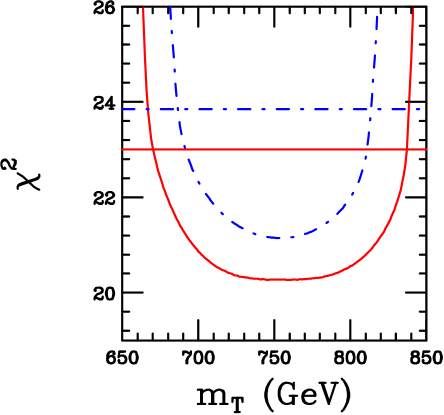
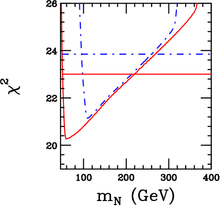
Figure 2: $\chi^{2}$ distributions at one (blue dotdash) and two loops (solid red), varying $m_{T}$ while marginalizing over $m_{N}$ (left) and varying $m_{N}$ while marginalizing over $m_{T}$ (right). $m_{B}=750$ and $m_{L}=200$ GeV are fixed. The horizontal lines indicate the corresponding 90% confidence intervals.

Figure 3 displays the 95% CL contour plots in the $(m_{L}-m_{N})$ – $(m_{T}-m_{B})$ plane. In these plots $m_{T}$ and $m_{N}$ are marginalized with $m_{L}=200$ GeV, $\theta_{34}=0$ and $m_{B}=600,750,900$ GeV. The one and two loop contours do not overlap, even for $m_{B}=600$ GeV, and become increasingly separated as the quark mass is increased. The two loop contours are larger than the one loop contours, as is apparent in figure 2.

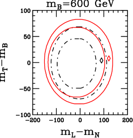
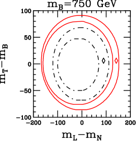
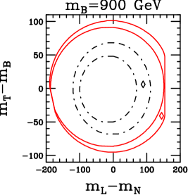
Figure 3: 95% CL contour plots computed with two loop (solid red) and one loop (blue dotdash) corrections with $m_{L}=200$ GeV, $m_{B}=600,750,900$ GeV, marginalizing over $m_{T}$ and $m_{N}$. Diamonds indicate the best fits.

The SM4 fits reflect an interplay between the quark and lepton contributions to $S$ and $T$. For $\theta_{34}=0$ the leading SM4 corrections are given entirely by $S$ and $T$, so that the oblique fit shown in table 1 and figure 1 is the limit for how good an SM4 fit can be. The SM4 fits then choose 4G masses to yield $S$ and $T$ as close as possible to the the best oblique fit, $S,T=0.055,0.08$. The quark contribution to $S$, which is rather insensitive to the specific values of $m_{T}$ and $m_{B}$, is large and positive, $S_{TB}\simeq 0.16$, well above the preferred value. It is offset by the lepton contribution to $S$ which includes a negative term proportional to $-{\rm log}(m_{L}/m_{N})$, favoring a large mass difference between $L$ and $N$ with $m_{L}>m_{N}$ as seen in figure 2. However large $(m_{L}-m_{N})$ induces a large positive contribution to $T$ that can force $S,T$ outside the 95% contour in figure 1. The fits then favor small $T,B$ mass splitting to minimize the quark contribution to $T$, and the $L,N$ mass difference strikes a balance to achieve the most negative possible contribution to $S$ while keeping $T$ from becoming too large. The importance of the two loop quark hypercharge correction is then apparent: because it makes a large negative contribution to $T$ it allows $(m_{L}/m_{N})$ to increase further, resulting in fits that more nearly approach the limiting value of the oblique fit.

$m_{B}$	600	750	900	$750:\ m_{T}$ [95%]
$m_{T}$	608	756	859	841.4
$m_{N}$	79	59	56	205.5
$S_{LN}$	-0.055	-0.10	-0.109	+0.057
$T_{L-N}^{(1)}$	0.25	0.334	0.35	0.00054
$T_{L-N}^{(2)}$	0.0019	0.0018	0.0017	0.0000071
$T_{LN}^{({\rm Y})}$	-0.00026	-0.00019	-0.00018	-0.0015
$T_{LN}^{({\rm TOT})}$	0.25	0.336	0.35	-0.00094
$S_{TB}$	0.158	0.16	0.164	0.147
$T_{T-B}^{(1)}$	0.0034	0.0019	0.090	0.45
$T_{T-B}^{(2)}$	0.00040	0.00035	0.023	0.099
$T_{TB}^{({\rm Y})}$	-0.14	-0.256	-0.38	-0.30
$T_{TB}^{({\rm TOT})}$	-0.14	-0.254	-0.27	+0.25
$S_{\rm TOT}$	0.10	0.06	0.055	0.20
$T_{\rm TOT}$	0.11	0.08	0.08	0.25

Table 2: First three columns: contributions to $S$ and $T$ for the best fits with $m_{L}=200$ and $m_{B}=600,750,900$ GeV, marginalizing over $m_{N}$ and $m_{T}$. Fourth column: $m_{L}=200$ and $m_{B}=750$ GeV with $m_{T}$ at its 95% CL upper limit.

These features are visible in table 2, which dissects the quark and lepton contributions to $S$ and $T$. For each fit $m_{L}=200$ GeV is fixed. The first three columns are for the best fits with $m_{B}=600,750,900$ GeV and the fourth is for $m_{B}=750$ GeV with $m_{T}$ at its 95% upper limit. For the three best fits the two loop hypercharge correction makes the dominant contribution to $T$, especially for $m_{B}=600$ and 750 GeV where the one loop quark contribution is negligible in comparison. At the 95% upper limit on $m_{T}$, in the fourth column, the hypercharge correction is comparable to although smaller than the one loop term. The best fit at $m_{B}=900$ GeV reaches the $S,T$ values of the oblique fit.

4. Convergence of the Perturbation Expansion

In this section we examine the sensitivity of the fits to uncertainty in the perturbation expansion, which increases with increasing quark mass. Because of the large contribution from the hypercharge correction, which only begins at two loops, the validity of the expansion cannot be judged simply by the difference between the one and two loop fits.

Consider for instance the fit with $m_{B}=600$ GeV in table 2. The one loop result, $T^{(1)}=0.25$, differs by more than a factor two from the total result at two loops , $T_{\rm TOT}=0.11$, but this difference tells us nothing about the convergence of the loop expansion. The one loop result is completely dominated by the leptonic contribution, for which perturbation theory is certainly reliable since $m_{L}$ and $m_{N}$ are well within the perturbative domain, as is explicitly evident from the negligible value of the leptonic two loop contributions to $T$ in the table. The quark contribution to $T$ is completely dominated by the quark hypercharge term, which is large because it is not suppressed by the near degeneracy of the $T$ and $B$ masses favored by the fits.

To assess the reliability of the expansion we need the next order contribution to the quark hypercharge term, a three loop correction that is not known. The best we can do is to use a conservative generic estimate of the loop expansion parameter, $~{}y_{Q}^{2}/4\pi^{2}$, where $y_{Q}=m_{Q}/v$ is the quark coupling to the Higgs boson and $v=247$ GeV. In particular we use the known ratio of the one and two loop quark corrections[26] that result from the mass difference of $T$ and $B$ for the case $|m_{T}-m_{B}|\ll m_{B}$, which is consistent with and just a factor 3/4 smaller than the generic estimate,

$$R_{12}={{T_{T-B}^{(2)}}\over{T_{T-B}^{(1)}}}={3\over 16\pi^{2}}{m_{Q}^{2}\over v^{2}}.$$

We then have $R_{12}=0.11,0.18,0.25$ for $m_{Q}=600,750,900$ GeV.

To exhibit the effect of uncertainty of this magnitude we compare fits that shift the hypercharge correction by a factor $\pm R_{12}$,

$$T_{TB}^{({\rm Y})}\to T_{TB}^{({\rm Y})}\cdot(1\pm R_{12}).$$

Figure 4 compares $\chi^{2}$ distributions with $T_{TB}^{({\rm Y})}$ rescaled as above for $m_{B}=750$ GeV and $m_{L}=200$ GeV, as in figure 2. The distributions are very similar over most of the allowed range in $m_{T}$ and $m_{N}$, with significant differences only near the upper and lower limits on $m_{T}$ and the lower limit on $m_{N}$. The rescaling of the hypercharge correction shifts the 95% limits on $m_{T}$ and $m_{N}$ by $~{}5$ GeV or less.

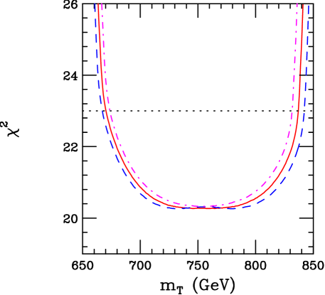
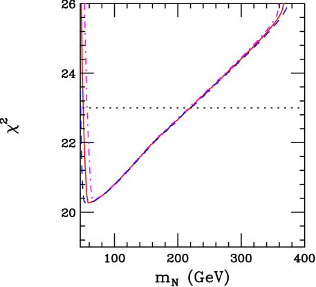
Figure 4: $\chi^{2}$ distributions computed at two loops with $T_{TB}^{({\rm Y})}$ rescaled by $1+R_{12}$ (blue dashes) and $1-R_{12}$ (magenta dotdash), compared with the central value (solid red). $m_{B}=750$ and $m_{L}=200$ GeV are fixed. The dotted lines mark the 90% confidence intervals.

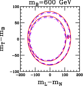
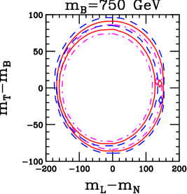
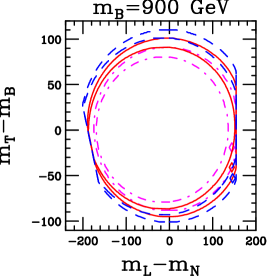
Figure 5: 95% CL contour plots , marginalizing over $m_{T}$ and $m_{N}$, computed at two loops with $T_{TB}^{({\rm Y})}$ rescaled by $1+R_{12}$ (blue dashes) and $1-R_{12}$ (magenta dotdash), compared with the central value (solid red). The charged lepton mass is fixed at $m_{L}=200$ GeV. Diamonds indicate the best fits.

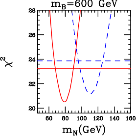
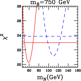
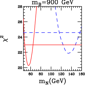
Figure 6: $\chi^{2}$ distributions as a function of $m_{N}$ with $m_{L}=200$ GeV and $m_{T}$ chosen as described in the text. The dashed blue and red distributions are from one and two loop fits respectively. The intersections of the distributions with the corresponding horizontal lines define the 90% confidence intervals for $m_{N}$.

Similarly, the contour plots in the $(m_{L}-m_{N})$ – $(m_{T}-m_{B})$ plane are compared in figure 5, for $m_{L}=200$ GeV and $m_{B}=600,750,900$ GeV, as in figure 3. For $m_{B}=600$ GeV the three contours overlap quite closely, even though 600 GeV exceeds the tree unitarity perturbative limit. For $m_{B}=750$ GeV they begin to diverge noticeably, as expected from the $\chi^{2}$ distributions in figure 4. Finally, for $m_{B}=900$ GeV the three 95% contours are almost completely non-overlapping, suggesting that perturbation theory may be of limited value at this mass scale.

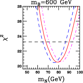
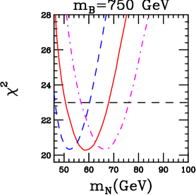
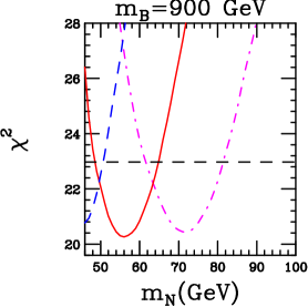
Figure 7: Two loop $\chi^{2}$ distributions as a function of $m_{N}$ with $m_{L}=200$ GeV and $m_{T}$ chosen as described in the text. The hypercharge correction $T_{TB}^{({\rm Y})}$ is rescaled by $1+R_{12}$ (blue dashes) and $1-R_{12}$ (magenta dotdash), compared with the central value (solid red). The horizontal lines indicate the 90% confidence intervals.

Finally we consider an example of how the electroweak corrections will be used in practice if evidence of a fourth generation is discovered at the LHC. We imagine that the $T$ and $B$ quarks and the charged lepton $L$ are discovered and their masses measured, and we consider how well the electroweak fit can then constrain the mass of the yet undiscovered heavy neutrino $N$. In figure 6 we compare the constraints for one and two loop fits, and in figure 7 we compare the two loop fits with $T_{TB}^{({\rm Y})}$ smeared as described above. We assume $m_{L}=200$ GeV and $m_{B}=600,750,900$ GeV. In each case $m_{T}$ is fixed at its value for the $\chi^{2}$ minimum obtained by marginalizing over $m_{T}$ and $m_{N}$, and $\chi^{2}$ is then obtained as a function of $m_{N}$.

$m_{B}$	Unsmeared	Smeared
600	68,90	65,93
750	51,68	46,76
900	48,65	46,81

Table 3: 90% confidence intervals for $m_{N}$ in GeV, as in figure 7. The unsmeared values are from the central (red) distributions in figure 7, while the smeared values are the outer envelopes of the distributions obtained by rescaling the hypercharge correction as described in the text.

We see in figure 6 that the 90% confidence intervals for $m_{N}$ of the one and two loop fits are completely disjoint, even for $m_{B}=600$ GeV, with increasing separation for larger $m_{B}$. In figure 7 we see that smearing the hypercharge correction by $1\pm R_{12}$ results in substantially overlapping confidence intervals for $m_{B}=600$ GeV that become almost completely disjoint for $m_{B}=900$ GeV. Table 3 shows the effect of the smearing on the 90% confidence intervals. For $m_{B}=600$ the impact of the smearing is modest, adding 3 GeV to the upper and lower limits. For $m_{B}=900$ GeV the effect is appreciable, with the 95% CL upper limit on $m_{N}$ increasing from 65 to 81 GeV. A comparable change would occur for the lower limit but is precluded by the direct lower limit on $m_{N}$ at 46 GeV.

5. Discussion

If the Higgs-like particle at 125 GeV is confirmed as the Higgs boson of the standard model, then SM4 appears to be excluded, although BSM4 variants with additional new quanta might still be viable. If it is a non-SM Higgs boson, e.g., a denizen of a 2HDM, then 4G models can also still be viable. We have used SM4 as a laboratory to study the effect of two loop corrections on the EW fit for 4G models. The results are qualitatively applicable to the broader class of 4G models, but detailed results can only be obtained from the examination of each particular model. For instance, for 2HDM models in regions of the parameter space with enhanced Yukawa coupling, the effect of the two loop hypercharge corrections could be even larger than the already large effect we have found in SM4.

In the SM4 “laboratory” we have identified an important two loop correction that has a big effect on the EW fit in 4G models. Although computed 25 years ago by van der Bij and Hoogeveen, it has not previously been included in EW fits of 4G models. It is important because it is the first correction that breaks the custodial $SU(2)$ even if weak doublet partners have equal mass, and, because it makes a large negative contribution to the rho parameter, it allows the fits to approach more closely to the limit of the oblique fit in which $S,T$ are free parameters. It is then important in the region of parameter space preferred by the EW fits, where the $T$ and $B$ quarks have nearly equal masses so that the one loop quark correction is small. In that experimentally preferred region it is by far the largest correction to the rho parameter from the 4G quark sector. Because of the hypercharge correction the two loop fits differ significantly from the one loop fits even when the quark masses are light enough that perturbation theory is reasonably convergent.

We have also studied the convergence of the perturbation expansion with increasing quark mass and its effect on the 4G contraints from the EW data, using a generic estimate of the order of magnitude of the three loop hypercharge correction, which is the largest unknown term in the parameter region preferred by the fits. We find that for $m_{Q}=600$ GeV perturbation theory provides useful guidance, even though tree unitarity for elastic $\overline{Q}Q$ scattering is saturated at at $m_{Q}=500$ GeV. For $m_{Q}=900$ GeV the estimated uncertainty increases so that it undermines the usefulness of the expansion. To obtain better etimates of the convergence of perturbation theory, it would be necessary to compute the the three loop hypercharge correction in the relevant models. Motivation to meet this challenge could be found if (and probably only if) evidence emerges for the existence of a fourth generation.

This work was supported in part by the Director, Office of Science, Office of High Energy and Nuclear Physics, Division of High Energy Physics, of the U.S. Department of Energy under Contract DE-AC02-05CH11231

References

- [1] M. Hashimoto, Phys.Rev.D81, 075023 (2010). arXiv:1001.4335
- [2] B. Holdom, Nuovo Cim. C035N3, 71 (2012). arXiv:1201.0074
- [3] O. Eberhardt , G. Herbert, H. Lacker, A. Lenz, A. Menzel et al., Phys.Rev.Lett. 109, 241802 (2012), arXiv:1209.1101 (2012). For analyses using earlier data sets see also O. Eberhardt, A. Lenz, A. Menzel, U. Nierste, and M. Wiebusch, Phys.Rev.D86, 074014 (2012), arXiv:1207.0438; O. Eberhardt, G. Herbert, H. Lacker, A. Lenz, A. Menzel, et al., Phys.Rev.D86, 013011 (2012); A. Djouadi and A. Lenz, Phys.Lett.B715, 310 (2012), arXiv:1204.1252; E. Kuflik, Y. Nir, T. Volansky(2012), arXiv:1204.1975. Crucial NLO corrections were obtained in G. Passarino, C. Sturm, S. Uccirati, Phys.Lett.B706 195 (2011), arXiv:1108.2025; and in A. Denner et al., Eur.Phys.J.C72 1992 (2012), arXiv:1111.6395.
- [4] B. Holdom, W.S. Hou et al., PMC Phys.A3, 4 (2009), arXiv:0904.4698; P. Frampton, P.Q. Hung, M. Sher, Phys.Rept.330, 263 (2000).
- [5] M. Geller, S. Bar-Shalom, G. Eilam, and A. Soni, arXiv:1209.4081 (2012); S. Bar-Shalom, M. Geller, S. Nandi, and A. Soni, arXiv:1208.3195 (2012); S. Bar-Shalom, S. Nandi, and A. Soni, Phys.Rev.{D84, 053009 (2011).
- [6] N. Chen and H.-J. He, JHEP 1204, 062 (2012), arXiv:1202.3072.
- [7] X.-G. He and G. Valencia, Phys.Lett. B707, 381 (2012), arXiv:1108.0222.
- [8] L. Bellantoni et al., Phys.Rev. D86 034022 (2012).
- [9] See for instance K. Agashe, R. Contino, A. Pomarol, Nucl.Phys. B719 165, (2005), arXiv:hep-ph/0412089; G. Giudice, C. Grojean, A. Pomarol, R. Rattazzi, JHEP 0706 045 (2007), arXiv:hep-ph/0703164; B. Bellazzini et al., arXiv:1205.4032 [hep-ph] (2102).
- [10] C.M. Ho, P.Q. Hung, T.W. Kephart, JHEP 1206, 045 (2012), arXiv:1102.3997; P.Q. Hung, C. Xiong, Phys.Lett. B694, 430 (2011), arXiv:0911.3892; P.Q. Hung, C. Xiong, Nucl.Phys. B847, 160 (2011), arXiv:0911.3890.
- [11] P.Q. Hung, C. Xiong, Nucl.Phys. B848, 288 (2011), arXiv:1012.4479.
- [12] W.D. Goldberger, B. Grinstein, Phys.Rev.Lett. 100, 111802 (2008); Z. Chacko, R.K. Mishra, arXiv:1209.3022 (2012); Z. Chacko, R. Franceschini, R.K. Mishra, arXiv:1209.3259 (2012); B. Bellazzini et al., arXiv:1209.3299 (2012); T. Abe et al., arXiv:1209.4544 (2012); S. Matsuzaki, K. Yamawaki, Phys.Rev. D85 095020 (2012), arXiv:1201.4722.
- [13] H.J. He, N. Polonsky, and S.F. Su, Phys.Rev. D64, 053004 (2001); V.A. Novikov, L.B. Okun, A.N. Rozanov, and M.I. Vysotsky, Phys. Lett. B529, 111 (2002); Pis’ma Zh. Eksp. Teor. Fiz. 76, 158 (2002); JETP Lett. 76, 127 (2002); G.D. Kribs, T. Plehn, M. Spannowsky, and T.M.P. Tait, Phys. Rev. D76, 075016 (2007).
- [14] M.S. Chanowitz, Phys. Rev. D79, 113008 (2009).
- [15] M. Frank, B. Korutlu, M. Toharia, Phys.Rev. D85 115025 (2012), arXiv:1204.5944.
- [16] CMS Collaboration, CMS-PAS-EXO-11-036, arXiv:submit/0449821 [hep-ex] (2011).
- [17] ATLAS Collaboration (Georges Aad et al.), arXiv:1210.5468 (2012).
- [18] CMS Collaboration (S. Chatrchyan et al.), Phys.Lett. B713, 408 (2012), arXiv:1205.0272.
- [19] J. Alwall et al., JHEP 1106, 128 (2011), arXiv:1106.0522.
- [20] J.M. Campbell, R. Fredrix, F. Maltoni, F. Tramontano, JHEP 0910, 042 (2009), arXiv:0907.3933; E.L. Berger, Q-H Cao, Phys. Rev. D81, 035006 (2010), arXiv:0909.3555.
- [21] K. Ishiwata, M.B. Wise, Phys.Rev. D83 074015 (2011) arXiv:1103.0611; T. Enkhbat, W-S Hou, H. Yokoya, Phys.Rev. D84, 094013 (2011), arXiv:1109.3382.
- [22] P.Q. Hung, M. Sher, Phys. Rev. D77, 037302 (2008); C.J. Flacco, D. Whiteson, T.M.P. Tait, S. Bar-Shalom (Technion), Phys.Rev.Lett. 105,111801 (2010), arXiv:1005.1077.
- [23] M.S. Chanowitz, M.A. Furman, I. Hinchliffe, Phys.Lett.B78:285,1978; Nucl.Phys.B153:402,1979.
- [24] M. Veltman, Nucl. Phys. B123, 89 (1977).
- [25] M. Peskin and T. Takeuchi, Phys. Rev. D46, 381 (1992).
- [26] J. Van der Bij and F. Hoogeveen, Nucl. Phys. B283, 477 (1987).
- [27] A. Freitas, Y.-C. Huang, JHEP 1208 050 (2012), arXiv:1205.0299.
- [28] The ALEPH, DELPHI, L3, OPAL, SLD Collaborations, the LEP Electroweak Working Group, the SLD Electroweak, and Heavy Flavour Groups, Phys. Rep. 427, 257 (2006). See http://lepewwg.web.cern.ch/ LEPEWWG/ for the most recent data.
- [29] A. B. Arbuzov et al., Comput. Phys. Commun. 174, 728 (2006).
- [30] M. Chanowitz, talk posted at http://www.ggi.fi.infn.it/talks/talk1452.pdf (2010).
- [31] B. Batell, S Gori, L.-T. Wang, arXiv:1209.6382.
- [32] H.-J. He, N. Polonsky, and S.-F. Su, Phys. Rev. D64, 053004 (2001).
- [33] H. Murayama et al., Phys.Lett. B705 208 (2011), arXiv:1012.0338.