Polymers in anisotropic environment with extended defects

Abstract

The conformational properties of flexible polymers in $d$ dimensions in environments with extended defects are analyzed both analytically and numerically. We consider the case, when structural defects are correlated in $\varepsilon_{d}$ dimensions and randomly distributed in the remaining $d-\varepsilon_{d}$. Within the lattice model of self-avoiding random walks (SAW), we apply the pruned-enriched Rosenbluth method (PERM) and find the estimates for scaling exponents and universal shape parameters of polymers in environment with parallel rod-like defects ($\varepsilon_{d}=1$). An analytical description of the model is developed within the des Cloizeaux direct polymer renormalization scheme.

1 Introduction

Conformational properties of polymer macromolecules in solutions are the subject of great interest in statistical polymer physics Gennes ; Grosberg ; Cloizaux90 . It is established, that long flexible polymers are characterized by a number of universal characteristics, independent of the chemical structure and architecture of the molecules. A typical example of such a quantity is the averaged end-to-end distance of $N$-monomer polymer chain (characterizing the linear size measure of macromolecule), that scales according to:

$$\langle R^{2}\rangle\sim N^{2\nu},$$ (1)

where $\nu$ is a universal exponent, depending on space dimension $d$ only ($\nu(d=3)=0.5877\pm 0.0006$ Li95 ). An other example is the rotationally invariant characteristic of the shape of typical polymer conformations, namely the aspherisity $\langle A_{d}\rangle$ Aronovitz86 , which equals $0$ for sphere-like shapes and $1$ for rod-like. For a polymer in a pure solvent in $d=3$ it was found $\langle A_{3}\rangle=0.431\pm 0.002$ Yagodzinski92 .

For a long time, the computer experiment served as the best tool to investigate polymer systems. In this approach, the most widely used model was and is until now the model of self-avoiding random walks (SAW) on a regular lattice. In spite of its simplicity, it perfectly captures the universal conformational properties of polymers in a solvent. Among the analytical descriptions of polymer systems the most successful are the field-theoretical approach Gennes , the direct polymer renormalization Cloizaux90 and the traditional Flory theory Gennes . The values of critical exponents and universal shape parameters, obtained within the frames of these theories, are in a good agreement with results of computer experiments.

The study of polymers in solvents in the presence of structural impurities plays a considerable role due to the importance to understand their behavior in colloidal solutions and near microporous membranes Cannel80 . It also connects with the description of proteins inside the living cells which can be treated as disordered environments Ellis03 . The behavior of polymers in disordered environments encountered controversies for a long time. During more than fifteen years there has been a wide discussion whether the presence of uncorrelated point-like defects leads to a change in universal properties Kremmer81 ; Chakrabarti81 ; Sahimi84 ; Lam84 ; Lyklema84 ; Lee88 ; Lee89 ; Kim90 ; Cherayil90 ; Roy90 ; Lam90 ; Kim91 ; Nakanishi91 ; Vanderzande92 . This problem was first posed by Kremer Kremmer81 showing that there exists a new value of the size exponent (1) only when the concentration of defects is above the percolation threshold. Later, this result was confirmed both analytically Kim83 and numerically Kim87 ; Woo91 ; Barat91 ; Grassberger93 ; Rintoul94 ; Lee96 ; Blavatska08 .

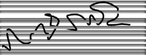
Figure 1: Schematic presentation of polymer chain in an environment with structural defects in form of parallel lines.

The density fluctuations of obstacles create large spatial inhomogeneities and pore spaces, which are often of fractal structure Dullen79 . A special case arises when fractal extended defects of parallel orientation are present in a system, which may cause the anisotropy of environment (see fig. 1). It is expected, that in this case there are two scaling exponents, governing the components of the size measure (1) in directions parallel and perpendicular to the orientadion of the extended defects Dorogovtsev80 ; Baumgaertner96 . The influence of such disorder on the critical behavior of magnetic systems with $\varepsilon_{d}$-dimensional defects of parallel orientation within frames of the spin $m-$vector model was analyzed in refs. Dorogovtsev80 ; Boyanovsky82 ; Blavatska02 . It was shown that there are two characteristic correlation lengths in the system, one parallel and other perpendicular to the defects. As it is known Gennes , the scaling properties of polymers in solution can be described within an $m-$vector model taking the de Gennes limit (polymer limit $m\to 0$).Unfortunatly, in the anisotropic case this approach does not give a satisfactory result.

In the present paper, we aim to obtain a quantitative description of the scaling behavior of polymer macromolecules in environments with $\varepsilon_{d}$-dimensional extended defects of parallel orientation (causing the anisotropy of environment), applying both numerical and analytical approaches. In the next Section, we study the special case of defects in form of randomly placed lines of parallel orientation ($\varepsilon_{d}=1$), applying computer simulations. In the Section 3, we develop an analytical description of the problem within the des Cloizeaux direct polymer renormalization scheme. We end giving conclusions and an outlook in Section 4.

2 Numerical analysis

2.1 The Method

We study the conformational properties of self-avoiding random walks on a regular lattice with extended impurities in the form of parallel lines (see fig. 1), applying the pruned-enriched Rosenbluth method (PERM) Grassberger97 . The method combines the original Rosenbluth-Rosenbluth algorithm of growing chains Rosenbluth55 and population control Wall59 . The $n$-th monomer is placed at a randomly chosen neighbor site of the previous $(n-1)$th monomer ($n\leq N$, where $N$ is total length of the polymer). If this randomly chosen site is already visited by a chain trajectory or belongs to an impurity line, it is avoided without discarding the chain and the weight $W_{n}$ given to each sample configuration at the $n$-th step is:

$$W_{n}=\prod_{l=1}^{n}m_{l},$$ (2)

where $m_{l}$ is the number of free lattice sites to place the $l$th monomer.

The growth is stopped when the total length $N$ of the chain is reached (or, at $n<N$, if a the “dead end” without possibility to make the next step is reached), then the next chain is started to grow from the starting point that is chosen randomly every time.

To derive appropriate properties of the chain we apply a two-step averaging: first average over configurations as usual and then averaging over different realizations of disorder. The configurational average for any quantity of interest then has the form:

$$\langle(\ldots)\rangle=\frac{1}{Z_{N}}{\sum_{k=1}^{M}W_{N}^{k}(\ldots)},\,\,\,\,Z_{N}=\sum_{k=1}^{M}W_{N}^{{\rm conf}},$$ (3)

where the summation is performed over the ensemble of all constructed $N$-step SAWs ($M\sim 10^{5}$ in our case). The disorder averaging is given in the form:

$${\overline{(\ldots)}}=\frac{1}{p}{\sum_{k=1}^{p}(\ldots)},$$ (4)

where $p$ is number of replicas (we take $p=400$ in our study).

The weight fluctuations of the growing chain are suppressed in PERM by pruning configurations with too small weights, and by enriching samples with copies of high-weight configurations. These copies are made while the chain is growing, and continue to grow independently of each other. Pruning and enrichment are performed by choosing thresholds $W_{n}^{<}$ and $W_{n}^{>}$, which are continuously updated as the simulation progresses. For updating the threshold values we apply similar rules as in Hsu03 ; Bachmann03 : $W_{n}^{>}=C(Z_{n}/Z_{1})(c_{n}/c_{1})^{2}$ and $W_{n}^{<}=0.2W_{n}^{>}$, where $c_{n}$ denotes the number of created chains having length $n$, and the parameter $C$ controls the pruning-enrichment statistics; it is adjusted such that on average 10 chains of total length $N$ are generated per each tour Bachmann03 .

2.2 Results and Discussions

We perform simulations for chains length up to $N=300$ monomers to measure the end-to-end distances and up to $N=100$ monomers for the asphericity value.

Let us introduce the position vectors ${\vec{r}}_{n}=\{x_{n}^{1},x_{n}^{2},x_{n}^{3}\}$ of each $n$-th monomer ($1\leq n\leq N$). In contrary to the the purely isotropic case (1), space anisotropy causes different scaling behavior for the end-to-end distance components in directions parallel ${\overline{\langle R^{2}_{\|}\rangle}}\equiv{\overline{\langle(x_{N}^{3}-x_{1}^{3})^{2}\rangle}}$ and perpendicular ${\overline{\langle R^{2}_{\|}\rangle}}\equiv{\overline{\langle(x_{N}^{1}-x_{1}^{1})^{2}+(x_{N}^{2}-x_{1}^{2})^{2}\rangle}}$ to the lines of defects (we assume, that the defects are extended in the $x^{3}$ direction). Namely:

$${\overline{\langle R^{2}_{\|}\rangle}}\sim N^{2\nu_{\|}},\,\,\,\qquad{\overline{\langle R^{2}_{\bot}\rangle}}\sim N^{2\nu_{\bot}},$$ (5)

with $\nu_{\|}\neq\nu_{\bot}$.

Analyzing our results for the end-to-end distance components the parallel and perpendicular to the lines of defects (see Fig. 2), we can see that when concentration of impurity lines is small, there is a crossover between two types of behavior: one for short length ($\sim 40$ monomers) and the other for longer chains. We can interpret this by the fact that at small concentration of defects the short chain does not feel the presence of impurities (when averaged distances between impurity lines approximately equal the length of the chain). In such situations, to calculate the value of size exponents we have to take into account only the second part as it is closer to the asymptotical regime.

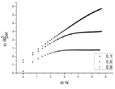
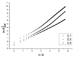
Figure 2: End-to-end distance component perpendicular (left) and parallel (right) to the impurity lines as functions of chain length in double logarithmic scale at several values of defects concentrations.

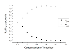
Figure 3: Size exponents (5) at various concentration of defects.

As it was suggested, there are two different size exponents $\nu_{\|}$ and $\nu_{\bot}$, which can be evaluated applying the least-square fitting of results presented in Fig. 2 to the form (5). For example, in the case of concentration 20 % we have $\nu_{\bot}=0.261\pm 0.005$ and $\nu_{\|}=0.86\pm 0.07$ which should be compared with corresponding pure value. Results for $\nu_{\bot}$, $\nu_{\|}$ at different concentrations of impurity lines are given in Fig. 3. Whereas exponent $\nu_{\|}$ gradually tends to the value of 1 as concentration of defects grows (the polymer chain extends in direction parallel to defects), the exponent $\nu_{\bot}$ is always smaller and gradually tends to zero.

To analyze the shape of polymers we calculate the components of gyration tensor given by:

$$Q_{ij}=\frac{1}{N^{2}}\sum_{m=1}^{N}\sum_{n=1}^{N}(x^{i}_{n}-x^{i}_{m})(x^{j}_{n}-x^{j}_{m})$$ (6)

where $i,j=1,2,3$. The shape of a typical polymer chain conformation can be described by a quantity:

$$A_{3}=\frac{3}{2}\frac{Tr\hat{Q}^{2}}{(TrQ)^{2}}\qquad\hat{Q}=Q-\hat{I}\frac{TrQ}{3}.$$ (7)

Our results for ${\overline{\langle A_{3}\rangle}}$ are given in Figure 4. One can see, that at small concentrations of impurity lines the polymer chain does not change its shape in spite of the existence of two different characteristic lengths. Increasing the defect concentration to medium concentrations the shape become more prolate and tends to a rod-like state.

As a result, polymers in an anisotropic environment with defects aligned in a given direction are elongated in this direction. In our case this is caused by the impurities that are extended along this direction and which repel the polymer.

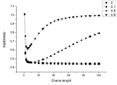
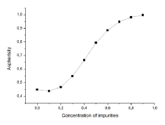
Figure 4: Aspheri ity as function of the chain length at several different concentrations of defects (left). The change of aspheri ity with increasing the defect concentration at fixed $N=100$ (right).

3 Analytical approach

Let us start with a continuous model, where the polymer chain is presented as a path parametrized by $\vec{r}(s)$, with $s=0\ldots S$. An effective Hamiltonian of the system is given by:

$$H=\frac{1}{2}\int^{S}_{0}\left(\frac{d\vec{r}(s)}{ds}\right)^{2}\,ds+u\int^{S}_{0}ds^{\prime}\int^{s^{\prime}}_{0}ds^{\prime\prime}\delta(\vec{r}(s^{\prime})-\vec{r}(s^{\prime\prime}))\,ds+$$

$$+\int^{S}_{0}\,V(\vec{r}(s))\,ds.$$ (8)

Note that $\vec{r}(s)$ is a $d$-dimentional vector with unit [length] while the parameters $S$, $s$ have units [length]². $S$ is also called the Gaussian surface. Here, the first term describes the chain connectivity, the second term reflects the excluded volume effect with coupling constant $u$, and the last term arises due to the interaction between the monomers of the polymer chain and the structural defects in the environment given by potential $V$.

We are interested in the case, when defects are correlated in $\varepsilon_{d}$ dimensions and randomly distributed in the remaining $d-\varepsilon_{d}$. The correlation function of the densities of defects is thus assumed to be given by Baumgaertner96 ; Dorogovtsev80 :

$${\overline{V(\vec{r}(s))V(\vec{r}(s^{\prime}))}}=v\delta^{d-\epsilon_{d}}(\vec{r}(s)-\vec{r}(s^{\prime})).$$ (9)

Averaging the partition sum of the model over different realizations of disorder with (9) results in:

$${\cal Z}_{{\rm dis}}=\int{\cal D}\{r\}\exp\left[-\frac{1}{2}\int^{S}_{0}\left(\frac{d\vec{r}(s)}{ds}\right)^{2}\,ds-u\int^{S}_{0}ds^{\prime}\int^{s^{\prime}}_{0}ds^{\prime\prime}\delta(\vec{r}(s^{\prime})-\vec{r}(s^{\prime\prime}))\,ds-\right.$$

$$\left.-v\int^{S}_{0}ds^{\prime}\int^{s^{\prime}}_{0}ds^{\prime\prime}\delta^{d-\epsilon_{d}}({r}_{d-\epsilon_{d}}(s^{\prime})-{r}_{d-\epsilon_{d}}(s^{\prime\prime}))\,ds\right],$$ (10)

Here, ${r}_{d-\epsilon_{d}}(s)$ denotes the component of position vector $\vec{r}(s)$ perpendicular to the orientation of the extended defects and the functional integration $\int{\cal D}\{r\}$ is to be performed over different chain configurations. Note that the coupling $u$ must be positive, which corresponds to an effective mutual repulsion of the monomers due to the excluded volume effect, whereas the coupling $v$ should have negative sign, weakening the covolume effect.

To evaluate quantitative estimates for the conformational characteristics of such a model, we apply the direct polymer renormalization scheme Cloizaux90 . All properties of interest can be found in the form of a perturbation theory series in an coupling constants. In particular, for the components of the end-to-end distances (5) we found:

$$R^{2}_{d-\epsilon_{d}}=S(d-\epsilon_{d})\left(1+\frac{z_{u}}{(2-\frac{d}{2})(3-\frac{d}{2})}+\frac{z_{v}}{(2-\frac{d-\epsilon_{d}}{2})(3-\frac{d-\epsilon_{d}}{2})}\right),$$ (11)

$$R^{2}_{\epsilon_{d}}=S\epsilon_{d}\left(1+\frac{z_{u}}{(2-\frac{d}{2})(3-\frac{d}{2})}\right),$$ (12)

here $z_{u}=u(2\pi)^{-d/2}S^{2-d/2}$ and $z_{v}=v(2\pi)^{-(d-\varepsilon_{d})/2}S^{2-(d-\varepsilon_{d})/2}$ are dimentionless couplinds. Note, that $\varepsilon_{d}$ indicates the dimentionality of the subspace parallel to the defects and $d-\varepsilon_{d}$ the dimentionality of the corresponding perpendicular subspace.

In the asymptotic limit $S\rightarrow\infty$ the physical quantities, presented in the form of series expansions in the coupling constants, are, however, divergent. To obtain asymptotical values of the corresponding physical parameters a renormalization of the coupling constants needs to be performed Cloizaux90 . The scaling exponents attain finite values when evaluated at the stable fixed point of the renormalization group transformation. The fixed points are defined as the common zeros of the flow equations, which in our problem read:

$$\beta_{u}=\epsilon z_{u}-8z_{u}^{2}-12z_{u}z_{v},$$

$$\beta_{v}=\delta z_{v}-8z_{v}^{2}-4z_{u}z_{v},$$ (13)

here $\epsilon=4-d$, $\delta=\epsilon+\varepsilon_{d}$. We find four fixed points:

$$z^{*}_{u}=0,\quad z^{*}_{v}=0,$$ (14)

$$z^{*}_{u}=\epsilon/8,\quad z^{*}_{v}=0,$$ (15)

$$z^{*}_{u}=0,\quad z^{*}_{v}=\delta/8,$$ (16)

$$z^{*}_{u}=\epsilon/2-3\,\delta/4,\quad z^{*}_{v}=\delta/2-\epsilon/4.$$ (17)

The first of them is the well known Gaussian fixed point, corresponding to an idealized polymer chain (random walk) without excluded volume interactions. The second describes another well known problem namely the polymer in a good solvent (disorder is absent). The third point describes the Gaussian polymer in an anisotropic environment and the last (most interesting one) describes SAW in anisotropic environment. Note, that at $\varepsilon_{d}=0$ we restore the situation with uncorrelated point-like defects, studied previously Kim83 ; Thirumalai88 ; Chakrabarti81 ; Cherayil90 . To correspond to a physical critical point of the system, the given fixed point should be stable and physically accessible. Unfortunately, in our problem the two last points, which are of main interest, are non-physical (e.g. attain appropriate values $z_{u}>0$ and $z_{v}<0$ only in the unphysical region $\varepsilon_{d}<0$) and thus, cannot provide estimates of scaling exponents. The same problem appears for the coupling flow functions of the $m-$vector model with extended defects Blavatska02 , when one tries to take the $m\rightarrow 0$ limit.

A similar problem of the absence of stable and physically accessible fixed points exists also in the case of uncorrelated point-like impurities Chakrabarti81 ; Cherayil90 , but it was solved by adsorbing the interaction with disorder into the excluded volume interaction due to special symmetry Kim83 . However it does not work in our case of extended defects. In spite of the problems evaluating numerical estimates of the critical exponents, our analytical work confirms the existence of two characteristic lengths for polymer in anisotropic environments.

4 Conclusions

We analyzed the conformational properties of flexible polymer chains in disordered anisotropic environments. The anisotropy is introduced in the form of $\varepsilon_{d}$-dimensional extended impurities of parallel orientation. Both numerical and analytical approaches are developed.

In numerical part of our work, we studied the scaling properties of a SAW model on a lattice with defects in a form of lines ($\varepsilon_{d}=1$), extended along a fixed coordinate direction. We conclude that there exist two critical exponents that describe the size measure of the polymer chain in directions parallel and perpendicular to the defects. The parallel exponent $\nu_{||}$ is always larger than the corresponding value for polymers in a pure solvent and gradually approaches the limit of 1 when increasing the defect concentration. The perpendicular exponent $\nu_{\perp}$ is always smaller and reaches the limit of 0. We also found, that increasing the concentration of defects, the shape of the polymers becomes more anisotropic, elongated in the direction parallel to the extended defects and gradually reaches the limit of a rod-like shape.

Our analytical study is developed on the basis of a continuous chain model with applying the direct polymer renormalization scheme. However, we encounter some controversies when analyzing stability and physical accessibility of fixed points, corresponding to a critical point of the system. Clarification of this problem will be the subject of our further work.

References

- (1) P.G. de Gennes, Scaling Concepts in Polymer Physics (Cornell University Press, Ithaca, 1979) 324.
- (2) A.Yu. Grosberg and A.R. Khokhlov, Statistical Physics of Macromolecules (AIP Press, New York, 1994).
- (3) J. des Cloizeaux, and G. Jannink, Polymers in Solutions: Their Modelling and Structure (Clarendon Press, Oxford, 1990) 886.
- (4) B Li, N Madras, and A D Sokal J. Stat. Phys. 80, (1995) 661
- (5) J.A. Aronovitz and D.R. Nelson, J. Physique 47 (1986) 1445.
- (6) O.Jagodzinski, E. Eisenriegler and K.Kremer, J. Phys. I (France) 2, (1992) 2243.
- (7) D.S. Cannel and F. Rondelez, Macromolecules 13, (1980) 1599.
- (8) R.J. Ellis and A.R. Minton, Nature 425, (2003) 27.
- (9) Kremer K., Z. Phys.,49, (1981) 149.
- (10) B.K. Chakrabarti and J. Kertesz, Z. Phys. B - Condensed Matter 44, (1981) 221-223
- (11) Muhammad Sahimi, J. Phys. A: Math. Gen. 17, (1984) L379-L384.
- (12) P. M. Lam, Z.Q. Zhang, Z. Phys. B - Condensed Matter 56, (1984) 155-159.
- (13) J.W. Lyklema and K. Kremer, Z. Phys. B - Condensed Matter 55, (1984) 41-44.
- (14) Sang Bub Lee and Hisao Nakanishi, Phys.Rev.Lett. 61, (1988) 2022.
- (15) Sang Bub Lee, Hisao Nakanishi and Y. Kim, Phys. Rev. B, 33, (1989) 9561.
- (16) Yup Kim, J. Phys. A: Math. Gen. 20, (1987) 1293-1297.
- (17) Binny J. Cherayil, J. Chem. Phys. 92, (1990) 6246.
- (18) A. K. Roy and A. Blumen, Journal of Statistical Physics 59, (1990) 1581.
- (19) P. M. Lam, J. Phys. A: Math. Gen. 23, (1990) L831-L836.
- (20) Yup Kim, Phys. Rev. A, 45, (1992) 6103.
- (21) Hisao Nakanishi and Sang Bub Lee, J. Phys. A: Math. Gen. 24 (1991) 1355-1361.
- (22) Carlo Vanderzande and Andrzej Komoda, Phys. Rev. A, 45, (1992) R5335.
- (23) Kim Y., J. Phys. C, 16,(1983) 1345.
- (24) Kim Y., J. Phys. A, 20, (1987) 1293.
- (25) Woo K. Y. and Lee S. B., Phys. Rev. A, 44, (1991) 999.
- (26) Barat K., Karmakar S. N. and Chakrabarti B. K., J. Phys. A, 1991, (1991) 851.
- (27) Grassberger P., J. Phys. A, 26, (1993) 1023.
- (28) M.C.Rintoul, Jangnyeol Moon and Hisao Nakanishi, Phys. Rev. E, 49, (1994) 2790.
- (29) Sang Bub Lee, Journal of Korea Physical Society 29, (1996) 1.
- (30) V. Blavatska and W. Janke, Europhys. Lett. 82, (2008) 66006; Phys. Rev. Lett. 101, (2008) 125701; J. Phys. A 42, (2009) 015001.
- (31) A.L. Dullen, Porous Media: Fluid Transport and Pore Structure (Academic, New York, 1979).
- (32) Dorogovtsev S.M., Fiz. Tverd. Tela(Leningrad), 22, (1980) 321.
- (33) A. Baumgartner and M. Muthukumar, Advances in Chemical Physics XCIV, (1996) 625-708.
- (34) Daniel Boyanovsky and John L. Cardy, Phys. Rev. B, 33,(1982) 154.
- (35) Blavatska V., C. von Ferber and Yu. Holovatch, Phys. Rev. B. 67 (2002) 094404; Acta Phys. Slov. 52, (2002) 317.
- (36) P. Grassberger, Phys. Rev. E 56, (1997) 3682.
- (37) M.N. Rosenbluth and A.W. Rosenbluth, J. Chem. Phys. 23,(1955) 356.
- (38) F.T. Wall and J.J. Erpenbeck, J. Chem. Phys. 30,(1959) 634 .
- (39) H.P. Hsu, V. Mehra, W. Nadler, and P. Grassberger, J. Chem. Phys. 118,(2007) 444 .
- (40) M. Bachmann and W. Janke, Phys. Rev. Lett. 91, (2003) 208105; J. Chem. Phys. 120, (2004) 6779.
- (41) D. Thirumalai, Phys. Rev. A, 37, (1988) 269.