Magnetic stripe domain pinning and reduction of in plane magnet order due to periodic defects in thin magnetic films

¹ School of Physics, The University of Western Australia, 35 Stirling Hwy, Crawley 6009, Australia
² SUPA School of Physics and Astronomy, University of Glasgow, Glasgow G12 8QQ, United Kingdom

Abstract

pacs: 75.30.Kz,64.70.dj,07.05.Tp,75.30.Cr
In thin magnetic films with strong perpendicular anisotropy and strong demagnetizing field two ordered phases are possible. At low temperatures, perpendicularly oriented magnetic domains form a striped pattern. As temperature is increased the system can undergo a spin reorientation transition into a state with in-plane magnetization. Here we present Monte Carlo simulations of such a magnetic film containing a periodic array of non-magnetic defects. We find that the presence of defects stabilizes parallel orientation of stripes against thermal fluctuations at low temperatures. Above the spin reorientation temperature we find that defects favor perpendicular spin alignment and disrupt long range ordering of spin components parallel to the sample. This increases cone angle and reduces in plane correlations, leading to a reduction in the spontaneous magnetization.

1 Introduction

Quasi two dimensional ultra thin magnetic films engender a large area of theoretical and technical interest, due in part to the large variety of magnetic properties that can be produced [1, 2] and their applications in data storage [3, 4]. For a sufficiently high ratio of dipole to exchange coupling strengths, the ground state of thin magnetic films can consist of magnetic stripe domains [5, 6, 7]. For films with a strong perpendicular anisotropy a second phase transition is possible, in which spins reorient resulting in a non zero magnetization parallel to the sample plane [8, 9, 10].
There are a number of lithographic techniques that can be used to create nanometer scale magnetic structures [11, 12, 13, 14, 15, 16, 17, 18, 19]. When compared with isotropic films, periodic magnetic nano structures have been shown to significantly alter macroscopic properties such as anisotropy [20, 21], magneto-resistance [20], cohesive field [22, 23] and spin reorientation temperature [24, 25].
On the micro scale, magnetic stripe domains can appear with long range orientaional order [7, 6, 26] or forming complex patterns [27, 6]. Nano scale patterning has been to used to create pinning sites for domain walls [28, 29, 30, 31, 32, 24]. When the period of pinning cites is comparable to the natural stripe width, long range orientational order can be stabilized [33, 24] .
Theoretically these quasi two dimensional systems have been studied with a variety of methods. For two dimensional isotropic systems the problem of melting is reasonably well understood [34], in particular the spin reorientation transition and stripe melting have been studied analytically [35, 36, 37, 38] and with computer simulation [39, 40, 41]. Theoretically the problem of melting in two dimensional systems has been considered for the case of particles with a periodic potential [42]. The pinning of domain walls has been explored for both random [43] and periodic defects[44]. Recently micro-magnetic computer simulations have explored the contribution of periodic defects and edge effects to magnetic reversal and hysteresis [45]. Here we perform Monte Carlo simulations on striped magnetic system in order understand the effect of periodic non magnetic defects on the thermally driven spin reorientation and stripe melting transitions.

2 Method

The system is modeled as a two dimensional square array of Heisenberg spins $\bm{s}_{\bm{i}}\in\mathcal{S}^{2}$, with lattice spacing $\alpha$.

$$\begin{split}H=&\frac{J}{2}\sum_{\langle\bm{i},\bm{j}\rangle}\bm{s}_{\bm{i}}\cdot\bm{s}_{\bm{j}}+K\sum_{\bm{i}}(s_{\bm{i}}^{z})^{2}\\ +&\frac{C_{D}}{2}\sum_{\bm{i},\bm{j}}\frac{1}{r_{\bm{\bm{ij}}}^{3}}(\bm{s}_{\bm{i}}\cdot\bm{s}_{\bm{j}}-3\bm{s}_{\bm{i}}\cdot\hat{\bm{r}}_{\bm{\bm{ij}}}\bm{s}_{\bm{j}}\cdot\hat{\bm{r}}_{\bm{\bm{ij}}})\end{split}$$ (1)

where $\bm{i}$ and $\bm{j}$ represent two dimensional indexes, $\bm{i}=(i_{x},i_{y})$, $s_{\bm{i}}^{z}=\bm{s}_{\bm{i}}\cdot\hat{\bm{z}}$ and $\langle\dots\rangle$ indicates the sum extends only over nearest neighbors. $J$, $K$ and $C_{D}$ represent the strength of the exchange coupling, perpendicular anisotropy and dipole coupling respectively. In order to introduce non-magnetic defects, some lattice sites are left empty. These defects are arranged as a regular square array with spacing $w_{d}$. The system is evaluated with Metropolis algorithm Monte Carlo. In order to approximate an infinite system, periodic boundary conditions are introduced. After the change of co-ordinates $\bm{r}_{\bm{nm}}=\bm{G}+\bm{\rho}_{\bm{n^{\prime}m^{\prime}}}$ where $\bm{\rho}_{\bm{n^{\prime}m^{\prime}}}=(\rho_{x},\rho_{y})$ and $\rho_{x},\rho_{y}\in[0,L]$, dipole coupling is calculated over a series of replicas of the original system [46, 47] the dipole interaction and Monte Carlo steps are parallelized on a GPU using the stream processing method described in our previous paper [41]. Non magnetic sites $\bm{s}_{\bm{i}}=\bm{0}$ are not updated.

3 Results

In order to create a periodic array of defects we select a system size of $L=64\alpha$ and defect spacing $w_{d}=8\alpha$. The ratio $\mathcal{K}=K/C_{D}$ was set as $\mathcal{K}=15$ ensuring that the ground state was not canted ($\bm{s}_{\bm{i}}\cdot\hat{\bm{z}}=\pm 1$). The ratio of exchange to dipole coupling is selected to be $\mathcal{J}=J/C_{D}=8.9$ giving a stripe width of $w_{s}=8\alpha$. At $T=0$, when the system is ordered, we find that for the choice of parameters above, the lowest energy occurs when domain boundaries pass through magnetic defects (this minimizes the energy by replacing a high energy spin with a defect). The system is initiated in the ground state and Monte Carlo ensembles are generated disregarding the initial $10^{5}$ Monte Carlo steps to allow the system to equilibrate. A further $5\times 10^{4}$ steps are taken with states recorded every $50$ steps. Previously we determined that $50$ steps allowed sufficient independence between ensemble configurations. In order to examine the effects of the defects results are included from an identical simulation performed on a perfect lattice that we shall refer to as the isotropic case.
When describing results we will refer to the normalized temperature $\mathcal{T}=k_{B}TC_{D}^{-1}$. In Fig. 1 sample states are shown for low temperatures near to where orientational order is destroyed. In the absence of defects, as $\mathcal{T}$ is increased, the striped system initially undergoes roughening at the stripe boundaries. The roughened domain boundaries are associated with localized canting of the spins away from perpendicular alignment. As temperature is further increased the system undergoes bridging between stripes that leads to the destruction of long range orientational order. With the inclusion of defects the same general trends occur: stripe roughening followed by bridging and eventual destruction of long range order. However, the presence of defects stabilizes the striped order at higher temperatures. In addition, differences in morphology are observed. In the absence of defects the stripes display long wavelength undulations. In the presence of defects walls are pinned. Instead of long wavelength bending, fluctuations exist as roughening of the sections of wall between defects. Also, in contrast to the isotropic case, we observe that this initial roughening of stripes is not associated with the appearance of canted spins.

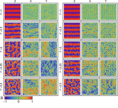
Figure 1: Example of spin configurations near the loss of orientational order. Spins vales are indicated according the color scale shown below, defects are colored black. Columns from left to right: $s_{\bm{i}}^{z}$, $s_{\bm{i}}^{x}$ and $s_{\bm{i}}^{y}$ followed by the same states in the presence of defects. Rows from top to bottom: $\mathcal{T}=1$, $\mathcal{T}=2.5$, $\mathcal{T}=3$, $\mathcal{T}=3.25$ and $\mathcal{T}=3.5$

In Fig. 2 the behavior of the two systems is shown at temperatures above the loss of orientational order. In both cases the system forms regions with spins canted towards in-plane alignment and the existence of long range order in the in-plane components. As temperature is increased the systems become increasing granular before reaching the paramagnetic limit.

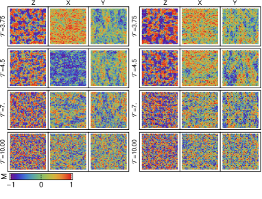
Figure 2: Example of spin configurations at high temperature. Colors are used to indicate spins values and the loation of defects as in Fig. 1. Columns from left to right: $s_{\bm{i}}^{z}$, $s_{\bm{i}}^{x}$ and $s_{\bm{i}}^{y}$ followed by the same states in the presence of defects.Rows from top to bottom: $\mathcal{T}=3.75$ , $\mathcal{T}=4.5$ ,$\mathcal{T}=7$ and $\mathcal{T}=10$

3.1 Orientational Order Parameter

In order to analyze the loss of orientational order we locate vertical and horizontal perpendicular domain walls by using $n_{h}^{z}$ and $n_{v}^{z}$ [40, 48, 41]

$$\begin{split}n_{h}^{z}&=\frac{1}{2N}\sum_{\bm{i,j}\>\text{v.n.n}}1-\text{sgn}(\bm{s}_{\bm{i}}\cdot\hat{\bm{z}}\;\bm{s}_{\bm{j}}\cdot\hat{\bm{z}})\\ n_{v}^{z}&=\frac{1}{2N}\sum_{\bm{i,j}\>\text{h.n.n}}1-\text{sgn}(\bm{s}_{\bm{i}}\cdot\hat{\bm{z}}\;\bm{s}_{\bm{j}}\cdot\hat{\bm{z}})\end{split}$$ (2)

where v.n.n and h.n.n indicate that the sums should be taken over all pairs of spins which are nearest neighbors in the horizontal and vertical directions respectively. The orientational order is given by

$$\mathcal{O}_{z}=\left\langle|n_{h}^{z}-n_{v}^{z}|/(n_{h}^{z}+n_{v}^{z})\right\rangle$$ (3)

With the inclusion of defects the sums in Eq. 2 are restricted to run over all pairs that are not defects.
In Fig. 3 $\mathcal{O}_{z}$ is plotted as a function of the normalized temperature $\mathcal{T}$.

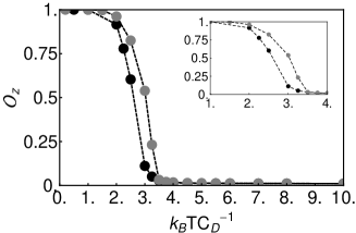
Figure 3: Orientational Order Parameter as a function of $\mathcal{T}$, black circles represent the uniform system, while gray dots represent the system in the presence of defects. The transition region is replotted with a finer $\mathcal{T}$ scale in the insert.

At low $\mathcal{T}$ both systems display a striped array with smooth boundaries corresponding to $\mathcal{O}_{z}=1$. We observe that, while the transition profile is similar, the presence of defects increases the transition temperature.

3.2 In Plane Magnetic Order

At high temperature when spins are no longer entirely perpendicular the system can display net magnetization parallel to the system plane. Letting $M_{x}=1/N\sum_{\bm{i}}s_{\bm{i}}^{x}$ and $M_{y}=1/N\sum_{\bm{i}}s_{\bm{i}}^{y}$ (with $N=L^{2}$) , the in plane magnetization is

$$M_{\parallel}=\langle(M_{x}^{2}+M_{y}^{2})^{\frac{1}{2}}\rangle.$$ (4)

In plane magnetic order can occur only when spins are canted away from the perpendicular alignment, in order to measure the degree of canting we use the cone angle

$$\begin{split}\eta&=\left\langle\frac{1}{N}\sum_{\bm{i}}\eta_{\bm{i}}\right\rangle\\ \text{with}\\ \eta_{\bm{i}}&=\sqrt{(2/\pi)^{2}\langle(\theta_{\bm{i}}-\pi/2)^{2}\rangle}\end{split}$$ (5)

where $\theta_{\bm{i}}$ is the zenith angle of the spin at site $\bm{i}$. When calculating $\eta$ and $M_{\parallel}$ in the presence of defects $N$ is replaced with $N^{\prime}=N(w_{d}^{2}-1)/w_{d}^{2}$ to account for the fact that the defects don’t contribute to the averages. In addition to these two single site order parameters, we calculate correlation functions between different spins. Taking $\theta_{\bm{i}}$ and $\phi_{\bm{i}}$ as the zenith and azimuthal angles of $\bm{s}_{\bm{i}}$ respectively, $\bm{s}_{\bm{i}}.\bm{s}_{\bm{j}}=\cos(\theta_{\bm{i}})\cos(\theta_{\bm{j}})+\sin(\theta_{\bm{i}})\sin(\theta_{\bm{j}})\cos(\phi_{\bm{i}}-\phi_{\bm{j}})$. Since we are interested in plane ordering we calculate

$$G_{\bm{ij}}=\begin{cases}\langle\cos(\phi_{\bm{i}}-\phi_{\bm{j}})\rangle&\text{for $\bm{s}_{\bm{i}}\neq 0$ and $\bm{s}_{\bm{j}}\neq 0$ }\\ 0&\text{otherwise}\end{cases}$$ (6)

In order to calculate the correlation as a function of distance we define

$$\begin{split}G_{\bm{i}}(r)=\frac{1}{N_{r}}\sum_{\bm{j}}\Pi((r_{\bm{ij}}-r)/\alpha)G_{\bm{ij}}\end{split}$$ (7)

Figure 4: The correlation between the circled sites on the left will not be equal to the correlation between the circled sites on the right due to the presence of a defect (indicated here by a black circle).

Here $\Pi$ is the Heaviside Pi function ($\Pi(x)=\Theta(x+1/2)\Theta(x-1/2)$) and $N_{r}$ is the number of spins contained in the average $G_{\bm{i}}(r)$; $N_{r}=\sum_{\bm{i}}\Pi((r_{\bm{ij}}-r)/\alpha)$. $G_{\bm{i}}(r)$ is the average correlation of the spin at site $\bm{i}$ with spins at a radius $r$ from $\bm{i}$. In a spatially isotropic state one expects that $G_{\bm{i}}(r)$ should depend only on the separation between spins. Here the inclusion of periodic defects breaks the isotropy. The correlation between two spins separated by distance $r$ will depend on the proximity of the spins to a defect. We define the following average; letting $n=(L/w_{d})$

$$\begin{split}\mathcal{G}_{\bm{i}}(r)&=\frac{1}{n^{2}}\sum_{\bm{i}^{\prime}=1}G_{\bm{i}^{\prime}}(r)=\frac{1}{n^{2}N_{r}}\sum_{\bm{i}^{\prime}=1}\sum_{\bm{j}}\Pi((r_{\bm{i}^{\prime}\bm{j}}-r)/\alpha)G_{\bm{i}^{\prime}\bm{j}}\\ \text{with}\\ \bm{i}^{\prime}&=\bm{i}+w_{d}a\hat{\bm{x}}+w_{d}b\hat{\bm{y}}\text{ for }a,b\in[1,n].\end{split}$$ (8)

The meaning of this correlation function is elucidated in Fig. 5. Here $G_{\bm{i}}(r)$ calculates the correlation between a fixed spin at site $\bm{i}$ and spins at some fixed distance $r$. Since the system is not spatially isotropic we expect that $G_{\bm{i}}(r)$ will depend on $\bm{i}$. $\mathcal{G}_{\bm{i}}(r)$ averages the $G_{\bm{i}}(r)$ over all sites with equivalent proximity to their closest defect. In the absence of the symmetry breaking defects and in a uniform phase $\mathcal{G}_{\bm{i}}(r)$ is not dependent on $\bm{i}$.

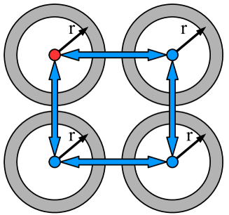
Figure 5: $G_{\bm{i}}(r)$ calculates the average correlation between the spin at site $\bm{i}$ (red circle) with all spins within a fixed radius (upper left gray circle). Spins separated by integer combinations of the vectors $w_{d}\hat{\bm{x}}$ $w_{d}\hat{\bm{y}}$ will have equivalent proximity to their nearest defect. $\mathcal{G}_{\bm{i}}(r)$ averages $G_{\bm{i}}(r)$ over these equivalent sites.

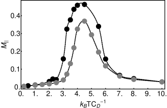
Figure 6: Parallel magnetization as a function of $\mathcal{T}$, black circles represent the uniform system, while gray dots represent the system in the presence of defects.

In Fig. 6 the parallel magnetization is shown as a function of temperature. Here we see that in the presence of defects the magnetic ordering is suppressed, and that the peak magnetization is reduced by around $20\%$. In Fig. 7 we see that the degree of spin canting is reduced for $2<\mathcal{T}<7$, however this reduced spin canting is not sufficient to account for the reduction in peak magnetization. In Fig. 8, $\mathcal{G}_{\bm{i}}(r)$ is plotted for $\mathcal{T}=4.5$, corresponding to the peak in-plane magnetization. In the isotropic system $\mathcal{G}_{\bm{i}}$ has slow monotonic decay with increasing distance between spins. For the non isotropic system $\mathcal{G}_{\bm{i}}$ is calculated for two choices of $\bm{i}$. The first choice is $\bm{i}$ as a nearest neighbor to a defect, in this case the correlation is strongly reduced for all $r$. The other choice is $\bm{i}$ at maximum distance from a defect, in this case the correlation is comparable to the isotropic case for small distances. However the correlation strength decreases rapidly as $r$ approaches $r=6\alpha$ (the location of the closest defects).
In addition to the reduction in correlation strength we observe a periodic structure in both the defect cases due to the periodic defect lattice. This effect is particularly strong for the case when the $\mathcal{G}_{\bm{i}}$ is calculated for $\bm{i}$ a maximum distance from defects, here certain values of $r$ will correspond to the average including several defects simultaneously. In order to gain a measure of the average effect of defects on magnetic correlation we also simulated the system with randomly located defects at $\mathcal{T}=4.5$. For this case we observe that $\mathcal{G}_{\bm{i}}$ lies between the results for the ordered defects described above.
In order to understand this reduced magnetic order close to the defects we show the spatial dependence of $\langle\eta_{\bm{i}}\rangle$ in Fig. 10 where we see that close to defects spins have a slightly increased average angle to the plane. In Fig. 9 this dependence is shown with randomly located defects. We observe the same local increase in cone angle near to defects. The effect is especially pronounced in the top left of the figure, where we observe a accumulation of defects associated with a region of significantly decreased canting.
When $w_{d}=8$ the average spacing between defects is large compared to the range of the local canting effect. In Fig. 8 we noted that, far from defects, short range correlations are comparable to those calculated for the isotropic system. In figures 12 and 13 we show the spacial dependence of $\langle\eta_{\bm{i}}\rangle$ with an increased defect density at $\mathcal{T}=4.5$. In the ordered case we have let $w_{d}=4$ and we see that the cone angle is no longer correlated with defect location. In contrast, when the same number of defects are randomly spaced as in Fig. 13, clustering leaves areas where the cone angle remains small.
In Fig. 11 we plot $\mathcal{G}_{\bm{i}}(r)$ for the high density defects. Unlike the low density case $\mathcal{G}_{\bm{i}}(r)$ does is not dependent on proximity to the ordered defects. We note also that the clustering effect means that the average short range correlation length is enhanced slightly when the defects are disordered. In all cases with high defect density the correlation length falls to zero at finite radius and so no in plane magnetization can form. In Table 1 we give the cone angle and magnetization for the cases described here and note that within the precision of the simulation, despite the differences in morphology and correlation length, the strength of the magnetic ordering is dependent on the density rather than periodicity of the defects.

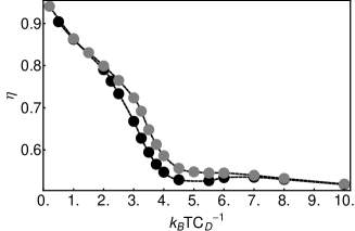
Figure 7: $\eta$ as a function of $\mathcal{T}$, black circles represent the uniform system, while gray dots represent the system in the presence of defects.

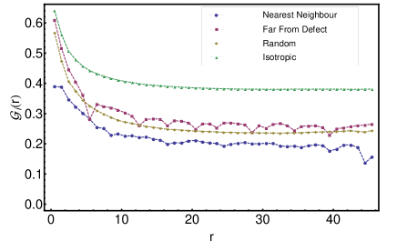
Figure 8: $\mathcal{G}_{\bm{i}}$ as a function of $r$ (given here in units of $\alpha$) at $\mathcal{T}=4.5$ for $\bm{i}$; as a nearest neighbor to ordered defects (blue circles), $\bm{i}$ at a maximum distance from ordered defects (red squares), in the presence of random defects (yellow diamonds) and for a defect free case (green triangles).

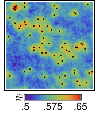
Figure 9: $\langle\eta_{\bm{i}}\rangle$ in the presence of randomly spaced defects at $\mathcal{T}=4.5$, black squares indicate defects and the value of $\eta_{\bm{i}}$ is indicated on the scale below.

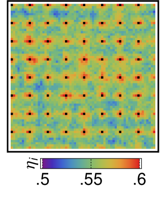
Figure 10: $\langle\eta_{\bm{i}}\rangle$ in the presence of regularly spaced defects at $\mathcal{T}=4.5$, black squares indicate defects and the value of $\eta_{\bm{i}}$ is indicated on the scale below.

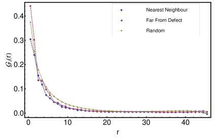
Figure 11: $\mathcal{G}_{\bm{i}}$ as a function of $r$ (given here in units of $\alpha$) at $\mathcal{T}=4.5$ in the presence of a high density of defects for $\bm{i}$; as a nearest neighbor to ordered defects (blue circles), $\bm{i}$ at a maximum distance from ordered defects (red squares) and in the presence of random defects (yellow diamonds).

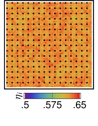
Figure 12: $\langle\eta_{\bm{i}}\rangle$ in the presence of closely spaced defects at $\mathcal{T}=4.5$, black squares indicate defects and the value of $\eta_{\bm{i}}$ is indicated on the scale below.

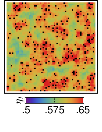
Figure 13: $\langle\eta_{\bm{i}}\rangle$ in the presence of regularly spaced defects at $\mathcal{T}=4.5$, black squares indicate defects and the value of $\eta_{\bm{i}}$ is indicated on the scale below.

Table 1: Comparison of the properties of isotropic system, ordered defects, and random defects at $\mathcal{T}=4.5$.

System	$M_{\parallel}$	$\eta$
Isotropic	0.463	0.529
Low Density Defects	0.363	0.556
Low Density Random Defects	0.359	0.556
High Density Defects	0.064	0.622
High Density Random Defects	0.080	0.614

3.3 Fluctuations

We now consider the effects of ordered low density defects on fluctuations as a function of $\mathcal{T}$. We calculate the autocorrelation function

$$\sigma^{2}(X)=\langle(X-\langle X\rangle)^{2}\rangle,$$ (9)

of the three order parameters $M_{\parallel}$, $\mathcal{O}^{z}$ and $\eta$, which we denote $\sigma^{2}_{\parallel}$, $\sigma^{2}_{\mathcal{O}}$ and $\sigma^{2}_{\eta}$ respectively. In Fig. 14 $\sigma^{2}_{\mathcal{O}}$is plotted as a function of $\mathcal{T}$, here we observe that the peak fluctuations occur at a higher temperature in the presence of defects corresponding to the stabilization of the striped structure.

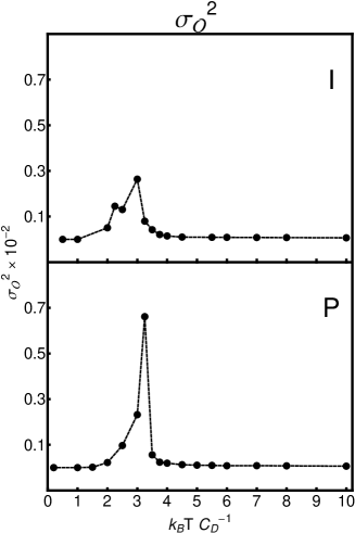
Figure 14: $\sigma^{2}_{\mathcal{O}}$ as a function of $\mathcal{T}$ for the isotropic case (I) and the patterned case (P).

$\sigma^{2}_{\parallel}$ as a function of $\mathcal{T}$ is plotted in Fig. 15. In both cases the fluctuations display two peaks corresponding to the creation and destruction of in-plane order. The low temperature peak is shifted towards higher $\mathcal{T}$ in the presence of defects.

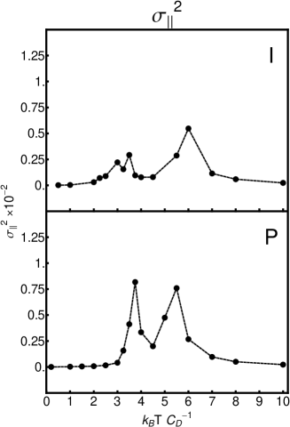
Figure 15: $\sigma^{2}_{\parallel}$ as a function of $\mathcal{T}$ for the isotropic case (I) and the patterned case (P).

In Fig. 16 $\sigma^{2}_{\eta}$ shows the same trend for both the patterned and isotropic cases, a broad peak with maximum occuring at $\mathcal{T}=4.5$ corresponding to the peak in-plane magnetic order.

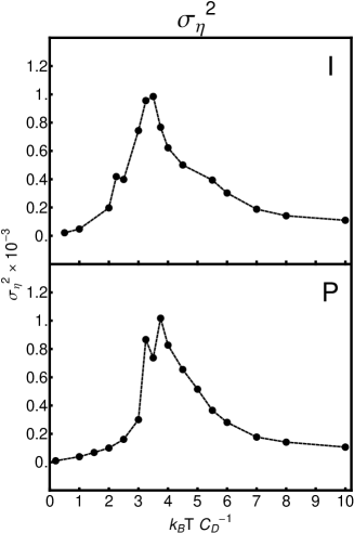
Figure 16: $\sigma^{2}_{\eta}$ as a function of $\mathcal{T}$ for the isotropic case (I) and the patterned case (P).

4 Conclusions and Comments

Monte Carlo simulations have been used to investigate the effects of non-magnetic defects on the stripe melting and spin reorientation transitions. We have shown that the inclusion of non magnetic defects with spacing comparable to the natural stripe width affects the melting of stripes by creating pinning sites for domain boundaries favoring parallel alignment of stripes. At higher temperatures the two measures of the spin reorientation transition (reduction of the cone angle and the appearance of in plane magnetization) are reduced. In particular there is a spatial dependence of cone angle and correlation strength on proximity to a defect. Recalling that dipole coupling favors in plane alignments of spins [39, 40], we surmise that the increased cone angle is due to the reduced dipole field near to the defects. The reduced dipole field increases the effective anisotropy near to the defects, suppressing canting away from perpendicular alignment. The increased $\eta$ values reduce the size of the $\sin(\theta_{\bm{i}})\sin(\theta_{\bm{j}})\cos(\phi_{\bm{i}}-\phi_{\bm{j}})$ term in $\bm{s}_{\bm{i}}.\bm{s}_{\bm{j}}$, effectively reducing the exchange coupling of the $x$ and $y$ components of the spins, leading to the suppression of in-plane magnetization.
Here we have restricted our attention to point defects. Recently Van de Wiele et al. have performed a temperature independent micro-magnetic simulation of magnetization reversal in a sample with square holes [45]. Here the defects have dimension comparable to the spacing between defects. They find that the local shape anisotropy of the holes significantly affects the reversal mechanism. In light of these calculations it would be interesting in the future to consider to consider the melting problem on larger lattices where the effects of changing the size and shape of defects could be investigated.

References

- [1] P.J. Jensen and K.H. Bennemann. Magnetic structure of films: Dependence on anisotropy and atomic morphology. Surface Science Reports, 61(3):129 – 199, 2006.
- [2] J. G. Gay and Roy Richter. Spin anisotropy of ferromagnetic films. Phys. Rev. Lett., 56:2728–2731, Jun 1986.
- [3] D. A. Thompson and J. S. Best. The future of magnetic data storage techology. IBM Journal of Research and Development, 44(3):311 –322, may 2000.
- [4] Mladen Todorovic, Sheldon Schultz, Joyce Wong, and Axel Scherer. Writing and reading of single magnetic domain per bit perpendicular patterned media. Applied Physics Letters, 74(17):2516 –2518, apr 1999.
- [5] F. C. Rossol. Temperature dependence of magnetic domain structure and wall energy in single-crystal thulium orthoferrite. Journal of Applied Physics, 39(11):5263–5267, 1968.
- [6] A. Vaterlaus, C. Stamm, U. Maier, M. G. Pini, P. Politi, and D. Pescia. Two-step disordering of perpendicularly magnetized ultrathin films. Phys. Rev. Lett., 84(10):2247–2250, Mar 2000.
- [7] G. Meyer, A. Bauer, T. Crecelius, I. Mauch, and G. Kaindl. Magnetization reversal via the formation of stripe domains in ultrathin fe films on cu(100). Phys. Rev. B, 68:212404, Dec 2003.
- [8] P. Politi, A. Rettori, M.G. Pini, and D. Pescia. Reorientation transition in a thin magnetic film. Journal of Magnetism and Magnetic Materials, 140–144, Part 1(0):647 – 648, 1995. International Conference on Magnetism.
- [9] R. Allenspach and A. Bischof. Magnetization direction switching in fe/cu(100) epitaxial films: Temperature and thickness dependence. Phys. Rev. Lett., 69(23):3385–3388, Dec 1992.
- [10] D. P. Pappas, K.-P. Kämper, and H. Hopster. Reversible transition between perpendicular and in-plane magnetization in ultrathin films. Phys. Rev. Lett., 64(26):3179–3182, Jun 1990.
- [11] J Fassbender, T Strache, M O Liedke, D Markó, S Wintz, K Lenz, A Keller, S Facsko, I Mönch, and J McCord. Introducing artificial length scales to tailor magnetic properties. New Journal of Physics, 11(12):125002, 2009.
- [12] M. Kostylev, R. Magaraggia, F.Y. Ogrin, E. Sirotkin, V.F. Mescheryakov, N. Ross, and R.L. Stamps. Ferromagnetic resonance investigation of macroscopic arrays of magnetic nanoelements fabricated using polysterene nanosphere lithographic mask technique. Magnetics, IEEE Transactions on, 44(11):2741 –2744, nov. 2008.
- [13] G.J. Li, C.W. Leung, Z.Q. Lei, K.W. Lin, P.T. Lai, and Philip W.T. Pong. Patterning of fept for magnetic recording. Thin Solid Films, 519(23):8307 – 8311, 2011. First International Conference of the Asian Union of Magnetics Societies (ICAUMS 2010).
- [14] J. F. Smyth, S. Schultz, D. Kern, H. Schmid, and Dennis Yee. Hysteresis of submicron permalloy particulate arrays. Journal of Applied Physics, 63(8):4237–4239, 1988.
- [15] Rachel Near, Christopher Tabor, Jinsong Duan, Ruth Pachter, and Mostafa El-Sayed. Pronounced effects of anisotropy on plasmonic properties of nanorings fabricated by electron beam lithography. Nano Letters, 12(4):2158–2164, 2012.
- [16] F. Rousseaux, D. Decanini, F. Carcenac, E. Cambril, M. F. Ravet, C. Chappert, N. Bardou, B. Bartenlian, and P. Veillet. Study of large area high density magnetic dot arrays fabricated using synchrotron radiation based x-ray lithography. Journal of Vacuum Science Technology B: Microelectronics and Nanometer Structures, 13(6):2787 –2791, nov 1995.
- [17] Henk Wolferen van and Leon Abelmann. Laser interference lithography. In Theodore C. Hennessy, editor, Lithography: Principles, Processes and Materials, pages 133–148. Nova Publishers, Hauppauge NY, USA, January 2011. Open Access.
- [18] Gang-Yu Liu, Song Xu, and Yile Qian. Nanofabrication of self-assembled monolayers using scanning probe lithography. Accounts of Chemical Research, 33(7):457–466, 2000.
- [19] J.I Martı́n, J Nogués, Kai Liu, J.L Vicent, and Ivan K Schuller. Ordered magnetic nanostructures: fabrication and properties. Journal of Magnetism and Magnetic Materials, 256(1–3):449 – 501, 2003.
- [20] F. J. Castano, K. Nielsch, C. A. Ross, J. W. A. Robinson, and R. Krishnan. Anisotropy and magnetotransport in ordered magnetic antidot arrays. Applied Physics Letters, 85(14):2872–2874, 2004.
- [21] P. Vavassori, G. Gubbiotti, G. Zangari, C. T. Yu, H. Yin, H. Jiang, and G. J. Mankey. Lattice symmetry and magnetization reversal in micron-size antidot arrays in permalloy film. Journal of Applied Physics, 91(10):7992–7994, 2002.
- [22] T. A. Moore, G. Wastlbauer, J. A. C. Bland, E. Cambril, M. Natali, D. Decanini, and Y. Chen. Antidot density-dependent reversal dynamics in ultrathin epitaxial fe/gaas(001). Journal of Applied Physics, 93(10):8746–8748, 2003.
- [23] H. Kronmüller. Theory of the coercive field in amorphous ferromagnetic alloys. Journal of Magnetism and Magnetic Materials, 24(2):159 – 167, 1981.
- [24] N. Bergeard, J. P. Jamet, A. Mougin, J. Ferré, J. Gierak, E. Bourhis, and R. Stamps. Dynamic fluctuations and two-dimensional melting at the spin reorientation transition. Phys. Rev. B, 86:094431, Sep 2012.
- [25] N. Bergeard, J.-P. Jamet, J. Ferre, A. Mougin, and J. Fassbender. Spin reorientation transition and phase diagram in an he[sup +] ion irradiated ultrathin pt/co(0.5 nm)/pt film. Journal of Applied Physics, 108(10):103915, 2010.
- [26] Y. Z. Wu, C. Won, A. Scholl, A. Doran, H. W. Zhao, X. F. Jin, and Z. Q. Qiu. Magnetic stripe domains in coupled magnetic sandwiches. Phys. Rev. Lett., 93:117205, Sep 2004.
- [27] H. P. Oepen, M. Speckmann, Y. Millev, and J. Kirschner. Unified approach to thickness-driven magnetic reorientation transitions. Phys. Rev. B, 55:2752–2755, Feb 1997.
- [28] R. P. Cowburn, A. O. Adeyeye, and J. A. C. Bland. Magnetic domain formation in lithographically defined antidot permalloy arrays. Applied Physics Letters, 70(17):2309–2311, 1997.
- [29] A. Perez-Junquera, G. Rodriguez-Rodriguez, M. Velez, J. I. Martin, H. Rubio, and J. M. Alameda. N[e-acute]el wall pinning on amorphous co[sub x]si[sub 1 - x] and co[sub y]zr[sub 1 - y] films with arrays of antidots in the diluted regime. Journal of Applied Physics, 99(3):033902, 2006.
- [30] G Rodríguez-Rodríguez, A Pérez-Junquera, M Vélez, J V Anguita, J I Martín, H Rubio, and J M Alameda. Mfm observations of domain wall creep and pinning effects in amorphous co x si 1− x films with diluted arrays of antidots. Journal of Physics D: Applied Physics, 40(10):3051, 2007.
- [31] P. J. Metaxas, P.-J. Zermatten, J.-P. Jamet, J. Ferre, G. Gaudin, B. Rodmacq, A. Schuhl, and R. L. Stamps. Periodic magnetic domain wall pinning in an ultrathin film with perpendicular anisotropy generated by the stray magnetic field of a ferromagnetic nanodot array. Applied Physics Letters, 94(13):132504, 2009.
- [32] Stan Konings, Jorge Miguel, Jeroen Goedkoop, Julio Camarero, and Jan Vogel. Magnetic domain pinning in an anisotropy-engineered gdtbfe thin film. Journal of Applied Physics, 100(3):033904, 2006.
- [33] Stan Konings, Jorge Miguel, Jeroen Luigjes, Hugo Schlatter, Huib Luigjes, Jeroen Goedkoop, and Vishwas Gadgil. Lock in of magnetic stripe domains to pinning lattices produced by focused ion-beam patterning. Journal of Applied Physics, 98(5):054306, 2005.
- [34] Katherine J. Strandburg. Two-dimensional melting. Rev. Mod. Phys., 60:161–207, Jan 1988.
- [35] P. J. Jensen and K. H. Bennemann. Direction of the magnetization of thin films and sandwiches as a function of temperature. Phys. Rev. B, 42:849–855, Jul 1990.
- [36] D. Pescia and V. L. Pokrovsky. Perpendicular versus in-plane magnetization in a 2d heisenberg monolayer at finite temperatures. Phys. Rev. Lett., 65:2599–2601, Nov 1990.
- [37] A. B. Kashuba and V. L. Pokrovsky. Stripe domain structures in a thin ferromagnetic film. Phys. Rev. B, 48:10335–10344, Oct 1993.
- [38] Ar. Abanov, V. Kalatsky, V. L. Pokrovsky, and W. M. Saslow. Phase diagram of ultrathin ferromagnetic films with perpendicular anisotropy. Phys. Rev. B, 51(2):1023–1038, Jan 1995.
- [39] Marianela Carubelli, Orlando V. Billoni, Santiago A. Pighín, Sergio A. Cannas, Daniel A. Stariolo, and Francisco A. Tamarit. Spin reorientation transition and phase diagram of ultrathin ferromagnetic films. Phys. Rev. B, 77(13):134417, Apr 2008.
- [40] J. P. Whitehead, A. B. MacIsaac, and K. De’Bell. Canted stripe phase near the spin reorientation transition in ultrathin magnetic films. Phys. Rev. B, 77:174415, May 2008.
- [41] M. Ambrose and R. L. Stamps. Untitled. October 2012.
- [42] David R. Nelson and B. I. Halperin. Dislocation-mediated melting in two dimensions. Phys. Rev. B, 19:2457–2484, Mar 1979.
- [43] V Zablotskii, J Ferré, and A Maziewski. Model for domain wall pinning by randomly distributed nanosized defects in ultrathin magnetic films. Journal of Physics D: Applied Physics, 42(12):125001, 2009.
- [44] A. M. Ettouhami and Leo Radzihovsky. Velocity-force characteristics of an interface driven through a periodic potential. Phys. Rev. B, 67:115412, Mar 2003.
- [45] B. Van de Wiele, A. Manzin, A. Vansteenkiste, O. Bottauscio, L. Dupre, and D. De Zutter. A micromagnetic study of the reversal mechanism in permalloy antidot arrays. Journal of Applied Physics, 111(5):053915, 2012.
- [46] Frank E. Harris. Ewald summations in systems with two-dimensional periodicity. International Journal of Quantum Chemistry, 68:385, Dec 1998.
- [47] P. P. Ewald. The calculation of optical and electrostatic grid potential. Annuals of Physics, 64:253, Apr 1921.
- [48] I. Booth, A. B. MacIsaac, J. P. Whitehead, and K. De’Bell. Domain structures in ultrathin magnetic films. Phys. Rev. Lett., 75(5):950–953, Jul 1995.