Uniformly accurate multiscale time integrators for highly oscillatory second order differential equations

Abstract

In this paper, two multiscale time integrators (MTIs), motivated from two types of multiscale decomposition by either frequency or frequency and amplitude, are proposed and analyzed for solving highly oscillatory second order differential equations with a dimensionless parameter $0<\varepsilon\leq 1$. In fact, the solution to this equation propagates waves with wavelength at $O(\varepsilon^{2})$ when $0<\varepsilon\ll 1$, which brings significantly numerical burdens in practical computation. We rigorously establish two independent error bounds for the two MTIs at $O(\tau^{2}/\varepsilon^{2})$ and $O(\varepsilon^{2})$ for $\varepsilon\in(0,1]$ with $\tau>0$ as step size, which imply that the two MTIs converge uniformly with linear convergence rate at $O(\tau)$ for $\varepsilon\in(0,1]$ and optimally with quadratic convergence rate at $O(\tau^{2})$ in the regimes when either $\varepsilon=O(1)$ or $0<\varepsilon\leq\tau$. Thus the meshing strategy requirement (or $\varepsilon$-scalability) of the two MTIs is $\tau=O(1)$ for $0<\varepsilon\ll 1$, which is significantly improved from $\tau=O(\varepsilon^{3})$ and $\tau=O(\varepsilon^{2})$ requested by finite difference methods and exponential wave integrators to the equation, respectively. Extensive numerical tests and comparisons with those classical numerical integrators are reported, which gear towards better understanding on the convergence and resolution properties of the two MTIs. In addition, numerical results support the two error bounds very well.

65L05, 65L20, 65L70 O2

1 Introduction

This paper is devoted to the study of numerical solutions of the following highly oscillatory second order differential equations (ODEs)

$$\left\{\begin{split}&\varepsilon^{2}\ddot{\mathbf{y}}(t)+A\mathbf{y}(t)+\frac{1}{\varepsilon^{2}}\mathbf{y}(t)+\mathbf{f}\left(\mathbf{y}(t)\right)=0,\quad t>0,\\ &\mathbf{y}(0)=\Phi_{1},\quad\dot{\mathbf{y}}(0)=\frac{\Phi_{2}}{\varepsilon^{2}}.\end{split}\right.$$ (1.1)

Here $t$ is time, $\mathbf{y}:=\mathbf{y}(t)=(y_{1}(t),\ldots,y_{d}(t))^{T}\in\mathbb{C}^{d}$ is a complex-valued vector function with $d$ a positive integer, $\dot{\mathbf{y}}$ and $\ddot{\mathbf{y}}$ refer to the first and second order derivatives of $\mathbf{y}$, respectively, $0<\varepsilon\leq 1$ is a dimensionless parameter which can be very small in some limit regimes, $A\in\mathbb{R}^{d\times d}$ is a symmetric nonnegative definite matrix, $\Phi_{1},\ \Phi_{2}\in\mathbb{C}^{d}$ are two given initial data at $O(1)$ in term of $0<\varepsilon\ll 1$, and $\mathbf{f}(\mathbf{y})=(f_{1}(\mathbf{y}),\ldots,f_{d}(\mathbf{y}))^{T}:\ \mathbb{C}^{d}\to\mathbb{C}^{d}$ describes the nonlinear interaction and it is independent of $\varepsilon$. The gauge invariance implies that $\mathbf{f}(\mathbf{y})$ satisfies the following relation [34]

$$\mathbf{f}(\mathrm{e}^{is}\mathbf{y})=\mathrm{e}^{is}\mathbf{f}(\mathbf{y}),\qquad\forall s\in\mathbb{R}.$$ (1.2)

We remak that when the initial data $\Phi_{1},\Phi_{2}\in\mathbb{R}^{d}$ and $\mathbf{f}(\mathbf{y}):\ \mathbb{R}^{d}\to\mathbb{R}^{d}$, then the solution $\mathbf{y}\in\mathbb{R}^{d}$ is real-valued. In this case, the gauge invariance condition (1.2) for the nonlinearity in (1.1) is no longer needed.

The above problem is motivated from our recent numerical study of the nonlinear Klein–Gordon equation in the nonrelativistic limit regime [5, 33, 34], where $0<\varepsilon\ll 1$ is scaled to be inversely proportional to the speed of light. In fact, it can be viewed as a model resulting from a semi-discretization in space, e.g., by finite difference or spectral discretization with a fixed mesh size (see detailed equations (3.3) and (3.19) in [5]), to the nonlinear Klein–Gordon equation. In order to propose new multiscale time integrators (MTIs) and compare with those classical numerical integrators including finite difference methods [5, 16, 39, 32] and exponential wave integrators [19, 36, 25, 26, 27] efficiently, we thus focus on the above second order differential equations instead of the original nonlinear Klein-Gordon equation. The solution to (1.1) propagates high oscillatory waves with wavelength at $O(\varepsilon^{2})$ and amplitude at $O(1)$. To illustrate this, Figure 1 shows the solutions of (1.1) with $d=2$, $f_{1}(y_{1},y_{2})=y_{1}^{2}y_{2}$, $f_{2}(y_{1},y_{2})=y_{2}^{2}y_{1}$, $A={\rm diag}(2,2)$, $\Phi_{1}=(1,0.5)^{T}$ and $\Phi_{2}=(1,2)^{T}$ for different $\varepsilon$. The highly oscillatory nature of solutions to (1.1) causes severe burdens in practical computation, making the numerical approximation extremely challenging and costly in the regime of $0<\varepsilon\ll 1$.

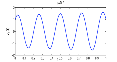
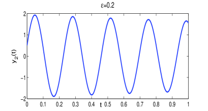
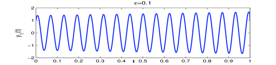
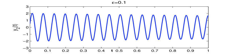
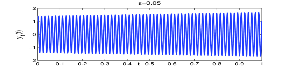
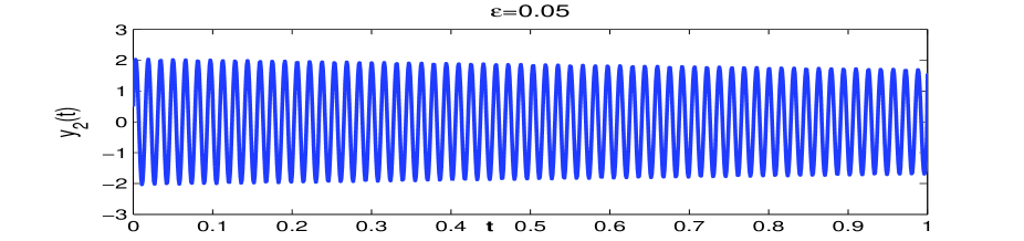
Figure 1: Time evolution of the solutions of (1.1) with $d=2$ for different $\varepsilon$.

For the global well-posedness of the model problem (1.1), we refer to [29, 30] and references therein. For simplicity of notations, we will present our methods and comparison for (1.1) in its simplest case, i.e. $d=1$, as

$$\left\{\begin{split}&\varepsilon^{2}\ddot{y}(t)+\left(\alpha+\frac{1}{\varepsilon^{2}}\right)y(t)+f\left(y(t)\right)=0,\quad t>0,\\ &y(0)=\phi_{1},\quad\dot{y}(0)=\frac{\phi_{2}}{\varepsilon^{2}},\end{split}\right.$$ (1.3)

where $y=y(t)\in\mathbb{C}$ is a complex-valued scalar function, $\alpha\geq 0$ is a real constant, $\phi_{1},\ \phi_{2}\in\mathbb{C}$, and $f(y):\ \mathbb{C}\to\mathbb{C}$. In particular, in many applications [21, 22, 23, 24, 33, 34, 38, 35, 37], $f(y)$ is taken as the pure power nonlinearity as

$$f(y)=g(|y|^{2})y,\ \hbox{with}\ g(\rho)=\lambda\rho^{p}\ \hbox{for some}\ \lambda\in\mathbb{R},\ p\in\mathbb{N}_{0}:=\mathbb{N}\cup\{0\}.$$ (1.4)

In addition, if $f$ is taken as the pure power nonlinearity (1.4), it is easy to see that (1.3) conserves the Hamiltonian or total energy, which is given by

$$E(t) := \varepsilon^{2}\left|\dot{y}(t)\right|^{2}+\left(\alpha+\frac{1}{\varepsilon^{2}}\right)\left|y(t)\right|^{2}+F\left(|y(t)|^{2}\right)$$ (1.5)

$$\equiv \frac{1}{\varepsilon^{2}}\left|\phi_{2}\right|^{2}+\left(\alpha+\frac{1}{\varepsilon^{2}}\right)\left|\phi_{1}\right|^{2}+F\left(|\phi_{1}|^{2}\right):=E(0),\quad t\geq 0,$$

with $F(\rho)=\int_{0}^{\rho}g(\rho^{\prime})d\rho^{\prime}$. Although the numerical methods and their error estimates in this paper are for the model problem (1.3), they can be easily extended to solve the problem (1.1). Similar to the nonlinear Klein-Gordon equation in the nonrelativistic limit regime [33, 34], when $0<\varepsilon\ll 1$, the total energy $E(t)=O(\varepsilon^{-2})$, i.e., it is unbounded when $\varepsilon\to 0$, with the given initial data in (1.3).

We remark here that the model problem (1.3) is quite different with the following oscillatory second order differential equation arising from molecular dynamics [26, 27, 11, 12, 36, 25]

$$\left\{\begin{split}&\ddot{y}(t)+\frac{1}{\varepsilon^{2}}y(t)+f(y(t))=0,\qquad t>0,\\ &y(0)=\varepsilon\phi_{1},\quad\dot{y}(0)=\phi_{2}.\end{split}\right.$$ (1.6)

In fact, the above problem (1.6) propagates waves with wave length and amplitude both at $O(\varepsilon)$, where the problem (1.3) propagates waves with wave length at $O(\varepsilon^{2})$ and amplitude at $O(1)$, and thus the oscillation in the problem (1.3) is much more oscillating and wild. In addition, dividing $\varepsilon^{2}$ on both sides of the model equation (1.3), we obtain

$$\ddot{y}+\frac{\alpha\varepsilon^{2}+1}{\varepsilon^{4}}y+\frac{1}{\varepsilon^{2}}f(y)=0.$$ (1.7)

Of course, when $\varepsilon=O(1)$, both (1.6) and (1.7) are perturbations to the harmonic oscillator. However, in the regime of $0<\varepsilon\ll 1$, due to the factor $\frac{1}{\varepsilon^{2}}$ in front of the nonlinear function, the nonlinear term in (1.7) is not a small perturbation to the harmonic oscillator! Resonance may occur at time $t=O(1)$. Another major difference is that the energy of the problem (1.6) is uniformly bounded for $\varepsilon\in(0,1]$, where it is unbounded in the problem (1.3) when $\varepsilon\to 0$. Different efficient and accurate numerical methods, including finite difference methods [5, 16], Gautschi type methods or exponential wave integrators (EWIs) [26, 11, 25], modified impulse methods [27, 12, 36], modulated Fourier expansion methods [27, 12, 36, 25], heterogeneous multiscale methods [17], flow averaging [41], Stroboscopic averaging [9] and Yong measure approach [1] have been proposed and analyzed as well as compared for the problem (1.6) in the literatures, especially in the regime when $0<\varepsilon\ll 1$. In addition, the modulated Fourier expansion has been developed as a powerful analytical tool for analyzing the oscillating structures of the problem (1.6) [11, 12, 25] and has been used to design numerical methods for the problem (1.6) and linear second-order ODEs with stiff source terms [11, 12, 36, 25, 13]. Based on the results in the literatures [26, 27, 11, 12, 36, 25], both the Gautschi type methods and modulated Fourier expansion methods preserve essentially the total energy and/or oscillatory energy over long times and converge uniformly for $\varepsilon\in(0,1]$ for the problem (1.6). However, based on the results in [5], all the above numerical methods do not converge uniformly for $\varepsilon\in(0,1]$ for the problem (1.3) which usually arise from quantum and plasma physics. In fact, for existing numerical methods to solve the problem (1.3), in order to capture ‘correctly’ the oscillatory solutions, one has to restrict the time step $\tau$ in a numerical integrator to be quite small when $0<\varepsilon\ll 1$. For instance, as suggested by the rigorous results in [5], for the frequently used finite difference (FD) time integrators in the literature [5, 16, 39], such as energy conservative, semi-implicit and explicit ones, the meshing strategy requirement (or $\varepsilon$-scalability) is $\tau=O(\varepsilon^{3})$ [5]. Also, a class of trigonometric integrators which solves the linear part of (1.3) exactly [5, 25, 26, 27, 36, 19], namely the exponential wave integrators (EWIs), require $\tau=O(\varepsilon^{2})$ for nonlinear problems [5]. In view of that the solutions to (1.3) are highly oscillatory with wavelength at $O(\varepsilon^{2})$, the EWIs could be viewed as the optimal one among the methods which integrate the oscillatory problem (1.3) directly.

The aim of this paper is to propose and analyze multiscale time integrators (MTIs) to the problem (1.3), which will converge uniformly for $\varepsilon\in(0,1]$ and thus possess much better improved $\varepsilon$-scalability than those classical FD and EWI methods in the regime $0<\varepsilon\ll 1$, by taking into account the sophisticated multiscale structures (see details in (2.2)) in frequency and/or amplitude of the solutions to (1.3). In our methods, at each time interval, we adopt an ansatz same as the one used in [33, 34], then carry out multiscale decompositions of the solution to (1.3) by either frequency or frequency and amplitude, and obtain a coupled equations for two $O(1)$-in-amplitude non-oscillatory components and an $O(\varepsilon^{2})$-in-amplitude oscillatory component. The coupled equations are then discretized by an explicit EWI method [25, 26, 27] with proper chosen transmission conditions between different time intervals. Our methods are different from the classical way of applying the modulated Fourier expansion methods for oscillatory ODEs [11, 12, 13] in terms of not only considering the leading order terms but also solving the equation of the remainder which is $O(\varepsilon^{2})$ in the pure power nonlinear case so as to design a uniformly convergent integrator for any $0<\varepsilon\leq 1$. For the MTIs, we rigorously establish two independent error bounds at $O(\tau^{2}/\varepsilon^{2})$ and $O(\varepsilon^{2})$ for $\varepsilon\in(0,1]$ by using the energy method and multiscale analysis [3, 4, 5]. These two error bounds immediately suggest that the MTIs converge uniformly with linear convergence rate at $O(\tau)$ for $\varepsilon\in(0,1]$ and optimally with quadratic convergence rate at $O(\tau^{2})$ in the regimes when either $\varepsilon=O(1)$ or $0<\varepsilon\leq\tau$. Thus, the MTIs offer compelling advantages over those FD and EWI methods for the problem (1.3), especially when $0<\varepsilon\ll 1$.

The rest of this paper is organized as follows. In Section 2, we present two multiscale decompositions for the solution of (1.3) by either frequency or frequency and amplitude. Two multiscale time integrators are proposed based on the two multiscale decompositions and their error bounds are established rigorously when the nonlinearity $f$ satisfies the power nonlinearity (1.4) and the general nonlinearity (1.2) in Sections 3 and 4, respectively. In Section 5, for comparison reasons, we present the classical FD and EWI discretizations to (1.3) and show their rigorous error analysis by paying particular attention on how error bounds depend on $\varepsilon$ explicitly. Numerical results are reported in Section 6. Finally, some concluding remarks are drawn in Section 7. Throughout this paper, we adopt the notation $A\lesssim B$ to represent that there exists a generic constant $C>0$, which is independent of $\tau$ (or $n$) and $\varepsilon$, such that $|A|\leq CB$.

2 Multiscale decompositions

Let $\tau=\Delta t>0$ be the step size, and denote time steps by $t_{n}=n\tau$ for $n=0,1,\ldots$ In this section, we present multiscale decompositions for the solution of (1.3) on the time interval $[t_{n},t_{n+1}]$ with given initial data at $t=t_{n}$ as

$$y(t_{n})=\phi_{1}^{n}=O(1),\qquad\dot{y}(t_{n})=\frac{\phi_{2}^{n}}{\varepsilon^{2}}=O\left(\frac{1}{\varepsilon^{2}}\right),$$ (2.1)

by either frequency or frequency and amplitude.

2.1 Multiscale decomposition by frequency (MDF)

Similar to the analytical study of the nonrelativistic limit of the nonlinear Klein-Gordon equation [33, 34], we take an ansatz to the solution $y(t):=y(t_{n}+s)$ of (1.3) on the time interval $[t_{n},t_{n+1}]$ with (2.1) as

$$y(t_{n}+s)=\mathrm{e}^{is/\varepsilon^{2}}z_{+}^{n}(s)+\mathrm{e}^{-is/\varepsilon^{2}}\overline{z_{-}^{n}}(s)+r^{n}(s),\qquad 0\leq s\leq\tau.$$ (2.2)

Here and after, $\bar{z}$ denotes the complex conjugate of a complex-valued function $z$. Differentiating (2.2) with respect to $s$, we have

$$\dot{y}(t_{n}+s)=\mathrm{e}^{is/\varepsilon^{2}}\left[\dot{z}_{+}^{n}(s)+\frac{i}{\varepsilon^{2}}z_{+}^{n}(s)\right]+\mathrm{e}^{-is/\varepsilon^{2}}\left[\overline{\dot{z}_{-}^{n}}(s)-\frac{i}{\varepsilon^{2}}\overline{z_{-}^{n}}(s)\right]+\dot{r}^{n}(s).$$ (2.3)

Plugging (2.2) into (1.3), we get

$$\left[2i\dot{z}_{+}^{n}(s)+\varepsilon^{2}\ddot{z}_{+}^{n}(s)+\alpha z_{+}^{n}(s)\right]\mathrm{e}^{is/\varepsilon^{2}}+\left[-2i\overline{\dot{z}_{-}^{n}}(s)+\varepsilon^{2}\overline{\ddot{z}_{-}^{n}}(s)+\alpha\overline{z_{-}^{n}}(s)\right]\mathrm{e}^{-is/\varepsilon^{2}}$$

$$\quad+\varepsilon^{2}\ddot{r}^{n}(s)+\left(\alpha+\frac{1}{\varepsilon^{2}}\right)r^{n}(s)+f\left(y(t_{n}+s)\right)=0,\qquad 0\leq s\leq\tau.$$ (2.4)

Multiplying the above equation by $\mathrm{e}^{-is/\varepsilon^{2}}$ and $\mathrm{e}^{is/\varepsilon^{2}}$, respectively, we can decompose the above equation into a coupled system for two $\varepsilon^{2}$-frequency waves with the unknowns $z_{\pm}^{n}(s)$ and the rest frequency waves with the unknown $r^{n}(s)$ as

$$\left\{\begin{split}&2i\dot{z}_{\pm}^{n}(s)+\varepsilon^{2}\ddot{z}_{\pm}^{n}(s)+\alpha z_{\pm}^{n}(s)+f_{\pm}\left(z_{+}^{n}(s),z_{-}^{n}(s)\right)=0,\quad 0<s\leq\tau,\\ &\varepsilon^{2}\ddot{r}^{n}(s)+\left(\alpha+\frac{1}{\varepsilon^{2}}\right)r^{n}(s)+f_{r}\left(z_{+}^{n}(s),z_{-}^{n}(s),r^{n}(s);s\right)=0,\end{split}\right.$$ (2.5)

where

$$f_{\pm}\left(z_{+},z_{-}\right)=\frac{1}{2\pi}\int_{0}^{2\pi}f\left(z_{\pm}+\mathrm{e}^{i\theta}\overline{z_{\mp}}\right)d\theta,$$ (2.6)

$$f_{r}\left(z_{+},z_{-},r;s\right)=f\left(\mathrm{e}^{is/\varepsilon^{2}}z_{+}+\mathrm{e}^{-is/\varepsilon^{2}}\overline{z_{-}}+r\right)-f_{+}\left(z_{+},z_{-}\right)\mathrm{e}^{is/\varepsilon^{2}}-\overline{f_{-}}\left(z_{+},z_{-}\right)\mathrm{e}^{-is/\varepsilon^{2}}.$$ (2.7)

In order to find proper initial conditions for the above system (2.5), setting $s=0$ in (2.2) and (2.3), noticing (2.1), we obtain

$$\left\{\begin{split}&z_{+}^{n}(0)+\overline{z_{-}^{n}}(0)+r^{n}(0)=y(t_{n})=\phi_{1}^{n},\\ &\frac{i}{\varepsilon^{2}}\left[z_{+}^{n}(0)-\overline{z_{-}^{n}}(0)\right]+\dot{z}_{+}^{n}(0)+\overline{\dot{z}_{-}^{n}}(0)+\dot{r}^{n}(0)=\dot{y}(t_{n})=\frac{\phi_{2}^{n}}{\varepsilon^{2}}.\end{split}\right.$$ (2.8)

Now we decompose the above initial data so as to: (i) equate $O\left(\frac{1}{\varepsilon^{2}}\right)$ and $O(1)$ terms in the second equation of (2.8), respectively, and (ii) be well-prepared for the first two equations in (2.5) when $0<\varepsilon\ll 1$, i.e. $\dot{z}_{+}^{n}(0)$ and $\dot{z}_{-}^{n}(0)$ are determined from the first two equations in (2.5), respectively, by setting $\varepsilon=0$ and $s=0$ [3, 4]:

$$\left\{\begin{split}&z_{+}^{n}(0)+\overline{z_{-}^{n}}(0)=\phi_{1}^{n},\qquad i\left[z_{+}^{n}(0)-\overline{z_{-}^{n}}(0)\right]=\phi_{2}^{n},\\ &2i\dot{z}_{\pm}^{n}(0)+\alpha z_{\pm}^{n}(0)+f_{\pm}\left(z_{+}^{n}(0),z_{-}^{n}(0)\right)=0,\\ &r^{n}(0)=0,\qquad\dot{r}^{n}(0)+\dot{z}_{+}^{n}(0)+\overline{\dot{z}_{-}^{n}}(0)=0.\end{split}\right.$$ (2.9)

Solving (2.9), we get the initial data for (2.5) as

$$\left\{\begin{split}&z_{+}^{n}(0)=\frac{1}{2}\left(\phi_{1}^{n}-i\phi_{2}^{n}\right),\qquad z_{-}^{n}(0)=\frac{1}{2}\left(\overline{\phi_{1}^{n}}-i\ \overline{\phi_{2}^{n}}\right),\\ &\dot{z}_{\pm}^{n}(0)=\frac{i}{2}\left[\alpha z_{\pm}^{n}(0)+f_{\pm}\left(z_{+}^{n}(0),z_{-}^{n}(0)\right)\right],\\ &r^{n}(0)=0,\qquad\dot{r}^{n}(0)=-\dot{z}_{+}^{n}(0)-\overline{\dot{z}_{-}^{n}}(0).\end{split}\right.$$ (2.10)

The above decomposition can be called as multiscale decomposition by frequency (MDF). In fact, it can also be regarded as to decompose slow waves at $\varepsilon^{2}$-wavelength and fast waves at other wavelengths, thus it can also be called as fast-slow frequency (FSF) decomposition.

Specifically, for pure power nonlinearity, i.e. $f$ satisfies (1.4), then the above MDF (2.5) collapses to

$$\left\{\begin{split}&2i\dot{z}_{\pm}^{n}(s)+\varepsilon^{2}\ddot{z}_{\pm}^{n}(s)+\alpha z_{\pm}^{n}(s)+g_{\pm}\left(|z_{+}^{n}(s)|^{2},|z_{-}^{n}(s)|^{2}\right)z_{\pm}^{n}(s)=0,\\ &\varepsilon^{2}\ddot{r}^{n}(s)+\left(\alpha+\frac{1}{\varepsilon^{2}}\right)r^{n}(s)+g_{r}\left(z_{+}^{n}(s),z_{-}^{n}(s),r^{n}(s);s\right)=0,\quad 0<s\leq\tau,\end{split}\right.$$ (2.11)

where

$$g_{\pm}\left(\rho_{+},\rho_{-}\right)=\sum_{\left\langle p_{1},p_{2},p_{3}\right\rangle_{0}}\lambda\left(\rho_{+}+\rho_{-}\right)^{p_{1}}(\rho_{+}\rho_{-})^{p_{2}}(\rho_{\mp})^{p_{3}},$$ (2.12)

$$g_{r}\left(z_{+},z_{-},r;s\right)=\sum_{k=1}^{p}\left(g_{k}\left(z_{+},z_{-}\right)\mathrm{e}^{i(2k+1)s/\varepsilon^{2}}+\overline{g_{k}}\left(z_{-},z_{+}\right)\mathrm{e}^{-i(2k+1)s/\varepsilon^{2}}\right)+h\left(z_{+},z_{-},r;s\right),$$ (2.13)

with

$$g_{k}\left(z_{+},z_{-}\right)=\lambda(z_{+})^{k+1}(z_{-})^{k}\sum_{\left\langle p_{1},p_{2},p_{3}\right\rangle_{k}}\left(|z_{+}|^{2}+|z_{-}|^{2}\right)^{p_{1}}|z_{+}|^{2p_{2}}|z_{-}|^{2p_{2}+2p_{3}},$$ (2.14)

$$h\left(z_{+},z_{-},r;s\right)=g\left(|\mathrm{e}^{is/\varepsilon^{2}}z_{+}+\mathrm{e}^{-is/\varepsilon^{2}}\overline{z_{-}}+r|^{2}\right)\left(\mathrm{e}^{is/\varepsilon^{2}}z_{+}+\mathrm{e}^{-is/\varepsilon^{2}}\overline{z_{-}}+r\right)$$

$$\qquad\qquad\qquad\ \ -g\left(|\mathrm{e}^{is/\varepsilon^{2}}z_{+}+\mathrm{e}^{-is/\varepsilon^{2}}\overline{z_{-}}|^{2}\right)\left(\mathrm{e}^{is/\varepsilon^{2}}z_{+}+\mathrm{e}^{-is/\varepsilon^{2}}\overline{z_{-}}\right),$$ (2.15)

and $\left\langle p_{1},p_{2},p_{3}\right\rangle_{k}=\left\{p_{1},p_{2},p_{3}\in\mathbb{N}_{0}\ \left|\ p_{1}+2p_{2}+p_{3}=p-k,\ p_{3}=0,1\right.\right\}$ for $k=0,\ldots,p$.

2.2 Multiscale decomposition by frequency and amplitude (MDFA)

Another way to decompose (2.1) is to decompose it into a coupled system for two $\varepsilon^{2}$-frequency waves at $O(1)$-amplitude with the unknowns $z_{\pm}^{n}(s)$ and the rest frequency and amplitude waves with the unknown $r^{n}(s)$ as

$$\left\{\begin{split}&2i\dot{z}_{\pm}^{n}(s)+\alpha z_{\pm}^{n}(s)+f_{\pm}\left(z_{+}^{n}(s),z_{-}^{n}(s)\right)=0,\qquad 0<s\leq\tau,\\ &\varepsilon^{2}\ddot{r}^{n}(s)+\left(\alpha+\frac{1}{\varepsilon^{2}}\right)r^{n}(s)+f_{r}\left(z_{+}^{n}(s),z_{-}^{n}(s),r^{n}(s);s\right)+\varepsilon^{2}u^{n}(s)=0,\end{split}\right.$$ (2.16)

where

$$u^{n}(s):=\mathrm{e}^{is/\varepsilon^{2}}\ddot{z}_{+}^{n}(s)+\mathrm{e}^{-is/\varepsilon^{2}}\overline{\ddot{z}_{-}^{n}}(s).$$ (2.17)

Similarly, the initial data (2.1) can be decomposed as the following for the coupled ODEs (2.16)

$$\left\{\begin{split}&z_{+}^{n}(0)=\frac{1}{2}\left(\phi_{1}^{n}-i\phi_{2}^{n}\right),\qquad z_{-}^{n}(0)=\frac{1}{2}\left(\overline{\phi_{1}^{n}}-i\ \overline{\phi_{2}^{n}}\right),\\ &r^{n}(0)=0,\qquad\dot{r}^{n}(0)=-\dot{z}_{+}^{n}(0)-\overline{\dot{z}_{-}^{n}}(0),\end{split}\right.$$ (2.18)

with

$$\dot{z}_{\pm}^{n}(0)=\frac{i}{2}\left[\alpha z_{\pm}^{n}(0)+f_{\pm}\left(z_{+}^{n}(0),z_{-}^{n}(0)\right)\right].$$

In the following, for simplicity of notations, we denote

$$f^{n}_{\pm}(s):=f_{\pm}(z^{n}_{+}(s),z_{-}^{n}(s)),\quad f_{r}^{n}(s):=f_{r}\left(z_{+}^{n}(s),z_{-}^{n}(s),r^{n}(s);s\right).$$ (2.19)

The above decomposition can be called as multiscale decomposition by frequency and amplitude (MDFA). In fact, it can also be regarded as to decompose large amplitude waves at $O(1)$ and small amplitude waves at $O(\varepsilon^{2})$, thus it can also be called as large-small amplitude (LSA) decomposition.

Similarly, for pure power nonlinearity, i.e. $f$ satisfies (1.4), then the above MDFA (2.16) collapses to

$$\left\{\begin{split}&2i\dot{z}_{\pm}^{n}(s)+\alpha z_{\pm}^{n}(s)+g_{\pm}\left(|z_{+}^{n}(s)|^{2},|z_{-}^{n}(s)|^{2}\right)z_{\pm}^{n}(s)=0,\quad 0<s\leq\tau,\\ &\varepsilon^{2}\ddot{r}^{n}(s)+\left(\alpha+\frac{1}{\varepsilon^{2}}\right)r^{n}(s)+g_{r}\left(z_{+}^{n}(s),z_{-}^{n}(s),r^{n}(s);s\right)+\varepsilon^{2}u^{n}(s)=0.\end{split}\right.$$ (2.20)

After solving the MDF (2.5) or (2.11) with the initial data (2.10), or the MDFA (2.16) or (2.20) with the initial data (2.18), we get $z_{\pm}^{n}(\tau)$, $\dot{z}_{\pm}^{n}(\tau)$, $r^{n}(\tau)$ and $\dot{r}^{n}(\tau)$. Then we can reconstruct the solution to (1.3) at $t=t_{n+1}$ by setting $s=\tau$ in (2.2) and (2.3), i.e.,

$$\left\{\begin{split}&y(t_{n+1})=\mathrm{e}^{i\tau/\varepsilon^{2}}z_{+}^{n}(\tau)+\mathrm{e}^{-i\tau/\varepsilon^{2}}\overline{z_{-}^{n}}(\tau)+r^{n}(\tau):=\phi_{1}^{n+1},\\ &\dot{y}(t_{n+1})=\frac{1}{\varepsilon^{2}}\phi_{2}^{n+1},\\ \end{split}\right.$$ (2.21)

with

$$\phi_{2}^{n+1}:=\mathrm{e}^{i\tau/\varepsilon^{2}}\left[\varepsilon^{2}\dot{z}_{+}^{n}(\tau)+iz_{+}^{n}(\tau)\right]+\mathrm{e}^{-i\tau/\varepsilon^{2}}\left[\varepsilon^{2}\overline{\dot{z}_{-}^{n}}(\tau)-i\overline{z_{-}^{n}}(\tau)\right]+\varepsilon^{2}\dot{r}^{n}(\tau).$$

3 Multiscale time integrators (MTIs) for pure power nonlinearity

Based on the decomposed system in the pure power nonlinearity case, i.e. the MDFA (2.20) or MDF (2.11), we propose two multiscale time integrators (MTI) for solving (1.3), respectively. At each time grid $t=t_{n}$, we solve the decomposed system (2.20) or (2.11) by proper integrators within the time interval $[0,\tau]$, and then use (2.21) to reconstruct the solution to (1.3) at $t=t_{n+1}$.

3.1 A MTI based on MDFA

Based on the MDFA (2.20), a MTI is designed as follows.

An exact integrator for $z_{\pm}^{n}(s)$ in (2.20):

Noting from (2.12) that $g_{\pm}\left(\rho_{+},\rho_{-}\right)$ is real-valued, similar to [6, 7], multiplying the first two equations in (2.20) by $\overline{z_{\pm}^{n}}(s)$, respectively, then subtracting from their complex conjugates, we have

$$\left|z_{\pm}^{n}(s)\right|\equiv\left|z_{\pm}^{n}(0)\right|,\qquad 0\leq s\leq\tau.$$ (3.1)

Therefore, the equations for $z^{n}_{\pm}(s)$ in (2.20) are exactly integrable, i.e.,

$$z_{\pm}^{n}(s)=\mathrm{e}^{{is}\left[g_{\pm}\left(|z_{+}^{n}(0)|^{2},|z_{-}^{n}(0)|^{2}\right)+\alpha\right]/2}z_{\pm}^{n}(0),\qquad 0\leq s\leq\tau.$$ (3.2)

Taking $s=\tau$ in (3.2), we get

$$z_{\pm}^{n}(\tau)=\mathrm{e}^{{i\tau}\left[g_{\pm}\left(|z_{+}^{n}(0)|^{2},|z_{-}^{n}(0)|^{2}\right)+\alpha\right]/2}z_{\pm}^{n}(0).$$ (3.3)

Differentiating (3.2) with respect to $s$ and then taking $s=0$ or $\tau$, we get

$$\left\{\begin{split}&\dot{z}_{\pm}^{n}(\tau)=\frac{i}{2}\left[g_{\pm}\left(|z_{+}^{n}(0)|^{2},|z_{-}^{n}(0)|^{2}\right)+\alpha\right]z_{\pm}^{n}(\tau),\\ &\ddot{z}_{\pm}^{n}(0)=-\frac{1}{4}\left[g_{\pm}\left(|z_{+}^{n}(0)|^{2},|z_{-}^{n}(0)|^{2}\right)+\alpha\right]^{2}z_{\pm}^{n}(0),\\ &\ddot{z}_{\pm}^{n}(\tau)=-\frac{1}{4}\left[g_{\pm}\left(|z_{+}^{n}(0)|^{2},|z_{-}^{n}(0)|^{2}\right)+\alpha\right]^{2}z_{\pm}^{n}(\tau).\end{split}\right.$$ (3.4)

An EWI for $r^{n}(s)$ in (2.20):

For the third equation in (2.20), we apply the exponential wave integrator (EWI) [4, 20, 25, 5, 27, 15, 26, 27, 36, 19] to solve it, which has favorable properties for solving the second-order oscillatory problems. By applying the variation-of-constant formula to $r^{n}(s)$, we get

$$r^{n}(s)=\frac{\sin(\omega s)}{\omega}\dot{r}^{n}(0)-\int_{0}^{s}\frac{\sin\left(\omega(s-\theta)\right)}{\varepsilon^{2}\omega}\left[g_{r}^{n}(\theta)+\varepsilon^{2}u^{n}(\theta)\right]d\theta,$$ (3.5)

where

$$\omega=\frac{\sqrt{1+\varepsilon^{2}\alpha}}{\varepsilon^{2}}=O\left(\frac{1}{\varepsilon^{2}}\right),\quad g_{r}^{n}(\theta):=g_{r}(z_{+}^{n}(\theta),z_{-}^{n}(\theta),r^{n}(\theta);\theta).$$ (3.6)

Taking $s=\tau$ in (3.5), we get

$$r^{n}(\tau)=\frac{\sin(\omega\tau)}{\omega}\dot{r}^{n}(0)-\int_{0}^{\tau}\frac{\sin\left(\omega(\tau-\theta)\right)}{\varepsilon^{2}\omega}\left[g_{r}^{n}(\theta)+\varepsilon^{2}u^{n}(\theta)\right]d\theta.$$ (3.7)

Differentiating (3.5) with respect to $s$ and then taking $s=\tau$, we get

$$\dot{r}^{n}(\tau)=\cos(\omega\tau)\dot{r}^{n}(0)-\int_{0}^{\tau}\frac{\cos\left(\omega(\tau-\theta)\right)}{\varepsilon^{2}}\left[g_{r}^{n}(\theta)+\varepsilon^{2}u^{n}(\theta)\right]d\theta.$$ (3.8)

Plugging (2.13) into (3.7) and (3.8), we find

$$\left\{\begin{split}&r^{n}(\tau)=\frac{\sin(\omega\tau)}{\omega}\dot{r}^{n}(0)-\sum_{k=1}^{p}\left[I^{n}_{k,+}+\overline{I^{n}_{k,-}}\right]-J^{n},\\ &\dot{r}^{n}(\tau)=\cos(\omega\tau)\dot{r}^{n}(0)-\sum_{k=1}^{p}\left[\dot{I}_{k,+}^{n}+\overline{\dot{I}^{n}_{k,-}}\right]-\dot{J}^{n},\end{split}\right.$$ (3.9)

where

$$\left\{\begin{split}&I_{k,\pm}^{n}=\int_{0}^{\tau}\frac{\sin(\omega(\tau-\theta))}{\varepsilon^{2}\omega}\mathrm{e}^{i(2k+1)\theta/\varepsilon^{2}}g_{k,\pm}^{n}(\theta)d\theta,\\ &J^{n}=\int_{0}^{\tau}\frac{\sin(\omega(\tau-\theta))}{\varepsilon^{2}\omega}\left[h^{n}(\theta)+\varepsilon^{2}u^{n}(\theta)\right]d\theta,\\ &\dot{I}_{k,\pm}^{n}=\int_{0}^{\tau}\frac{\cos(\omega(\tau-\theta))}{\varepsilon^{2}}\mathrm{e}^{i(2k+1)\theta/\varepsilon^{2}}g_{k,\pm}^{n}(\theta)d\theta,\\ &\dot{J}^{n}=\int_{0}^{\tau}\frac{\cos(\omega(\tau-\theta))}{\varepsilon^{2}}\left[h^{n}(\theta)+\varepsilon^{2}u^{n}(\theta)\right]d\theta,\end{split}\right.$$ (3.10)

with

$$g_{k,\pm}^{n}(\theta):=g_{k}(z_{\pm}^{n}(\theta),z_{\mp}^{n}(\theta)),\qquad h^{n}(\theta):=h\left(z_{+}^{n}(\theta),z_{-}^{n}(\theta),r^{n}(\theta);\theta\right).$$ (3.11)

In order to have an explicit integrator and achieve uniform error bounds, we approximate the integral terms $I_{k,\pm}^{n}$ and $\dot{I}_{k,\pm}^{n}$ in (3.10) by a quadrature in the Gautschi’s type [20] as the following which was discussed and used in [4, 5]

$$\left\{\begin{split}&I_{k,\pm}^{n}\approx\int_{0}^{\tau}\frac{\sin(\omega(\tau-\theta))}{\varepsilon^{2}\omega}\mathrm{e}^{i(2k+1)\theta/\varepsilon^{2}}\left[g_{k,\pm}^{n}(0)+\theta\dot{g}_{k,\pm}^{n}(0)\right]d\theta\\ &\qquad\ =p_{k}g_{k,\pm}^{n}(0)+q_{k}\dot{g}_{k,\pm}^{n}(0),\\ &\dot{I}_{k,\pm}^{n}\approx\int_{0}^{\tau}\frac{\cos(\omega(\tau-\theta))}{\varepsilon^{2}}\mathrm{e}^{i(2k+1)\theta/\varepsilon^{2}}\left[g_{k,\pm}^{n}(0)+\theta\dot{g}_{k,\pm}^{n}(0)\right]d\theta\\ &\qquad\ =\dot{p}_{k}g_{k,\pm}^{n}(0)+\dot{q}_{k}\dot{g}_{k,\pm}^{n}(0),\\ \end{split}\right.$$ (3.12)

where (their detailed explicit formulas are shown in Appendix A)

$$p_{k}=\int_{0}^{\tau}\frac{\sin(\omega(\tau-\theta))}{\varepsilon^{2}\omega}\mathrm{e}^{i(2k+1)\theta/\varepsilon^{2}}d\theta,\quad q_{k}=\int_{0}^{\tau}\frac{\sin(\omega(\tau-\theta))}{\varepsilon^{2}\omega}\mathrm{e}^{i(2k+1)\theta/\varepsilon^{2}}\theta d\theta,$$

$$\dot{p}_{k}=\int_{0}^{\tau}\frac{\cos(\omega(\tau-\theta))}{\varepsilon^{2}}\mathrm{e}^{i(2k+1)\theta/\varepsilon^{2}}d\theta,\quad\dot{q}_{k}=\int_{0}^{\tau}\frac{\cos(\omega(\tau-\theta))}{\varepsilon^{2}}\mathrm{e}^{i(2k+1)\theta/\varepsilon^{2}}\theta d\theta.\ \$$

In addition, approximating $J^{n}$ and $\dot{J}^{n}$ in (3.10) by the standard single step trapezoidal rule and noticing $h^{n}(0)=0$, we get

$$\left\{\begin{split}&J^{n}\approx\frac{\tau}{2}\frac{\sin(\omega\tau)}{\varepsilon^{2}\omega}\left[h^{n}(0)+\varepsilon^{2}u^{n}(0)\right]=\frac{\tau}{2}\frac{\sin(\omega\tau)}{\omega}u^{n}(0),\\ &\dot{J}^{n}\approx\frac{\tau}{2}\left[\frac{\cos(\omega\tau)}{\varepsilon^{2}}\left(h^{n}(0)+\varepsilon^{2}u^{n}(0)\right)+\frac{1}{\varepsilon^{2}}\left(h^{n}(\tau)+\varepsilon^{2}u^{n}(\tau)\right)\right].\end{split}\right.$$ (3.13)

Plugging (3.12), (3.13) and (3.10) into (3.9) and noticing $h^{n}(0)=0$, we obtain

$$\left\{\begin{split}&r^{n}(\tau)\approx-\sum_{k=1}^{p}\left[p_{k}g_{k,+}^{n}(0)+q_{k}\dot{g}_{k,+}^{n}(0)+\overline{p_{k}g_{k,-}^{n}(0)}+\overline{q_{k}\dot{g}_{k,-}^{n}(0)}\right]\\ &\ \qquad\quad+\frac{\sin(\omega\tau)}{\omega}\left[\dot{r}^{n}(0)-\frac{\tau}{2}u^{n}(0)\right],\\ &\dot{r}^{n}(\tau)\approx-\sum_{k=1}^{p}\left[\dot{p}_{k}g_{k,+}^{n}(0)+\dot{q}_{k}\dot{g}_{k,+}^{n}(0)+\overline{\dot{p}_{k}g_{k,-}^{n}(0)}+\overline{\dot{q}_{k}\dot{g}_{k,-}^{n}(0)}\right]\\ &\ \qquad\quad+\cos(\omega\tau)\left[\dot{r}^{n}(0)-\frac{\tau}{2}u^{n}(0)\right]-\frac{\tau}{2}\left[\frac{h^{n}(\tau)}{\varepsilon^{2}}+u^{n}(\tau)\right].\end{split}\right.$$ (3.14)

Detailed numerical scheme

For $n=0,1,\ldots,$ let $y^{n}$ and $\dot{y}^{n}$ be the approximations of $y(t_{n})$ and $\dot{y}(t_{n})$, $z_{\pm}^{n+1}$, $\dot{z}_{\pm}^{n+1}$, $\ddot{z}_{\pm}^{n+1}$, $r^{n+1}$ and $\dot{r}^{n+1}$ be the approximations of $z_{\pm}^{n}(\tau)$, $\dot{z}_{\pm}^{n}(\tau)$, $\ddot{z}_{\pm}^{n}(\tau)$, $r^{n}(\tau)$ and $\dot{r}^{n}(\tau)$, respectively, where $z_{\pm}^{n}(s)$ and $r^{n}(s)$ are the solutions to the system (2.20) with initial data (2.18). Choosing $y^{0}=y(0)=\phi_{1}$ and $\dot{y}^{0}=\dot{y}(0)=\varepsilon^{-2}\phi_{2}$, for $n=0,1,\ldots$, $y^{n+1}$ and $\dot{y}^{n+1}$ are updated as follows:

$$\left\{\begin{split}&y^{n+1}=\mathrm{e}^{i\tau/\varepsilon^{2}}z_{+}^{n+1}+\mathrm{e}^{-i\tau/\varepsilon^{2}}\overline{z_{-}^{n+1}}+r^{n+1},\\ &\dot{y}^{n+1}=\mathrm{e}^{i\tau/\varepsilon^{2}}\left(\dot{z}_{+}^{n+1}+\frac{i}{\varepsilon^{2}}z_{+}^{n+1}\right)+\mathrm{e}^{-i\tau/\varepsilon^{2}}\left(\overline{\dot{z}_{-}^{n+1}}-\frac{i}{\varepsilon^{2}}\overline{z_{-}^{n+1}}\right)+\dot{r}^{n+1},\end{split}\right.$$ (3.15)

where

$$z_{\pm}^{n+1}=\mathrm{e}^{i\mu_{\pm}\tau}z_{\pm}^{(0)},\qquad\dot{z}_{\pm}^{n+1}=i\mu_{\pm}z_{\pm}^{n+1},\qquad\ddot{z}_{\pm}^{n+1}=-(\mu_{\pm})^{2}z_{\pm}^{n+1},$$

$$r^{n+1}=\frac{\sin(\omega\tau)}{\omega}\left(\dot{r}^{(0)}-\frac{\tau}{2}u^{(0)}\right)-\sum_{k=1}^{p}\left[p_{k}g_{k,+}^{(0)}+q_{k}\dot{g}_{k,+}^{(0)}+\overline{p_{k}g_{k,-}^{(0)}}+\overline{q_{k}\dot{g}_{k,-}^{(0)}}\right],$$

$$\dot{r}^{n+1}=-\sum_{k=1}^{p}\left[\dot{p}_{k}g_{k,+}^{(0)}+\dot{q}_{k}\dot{g}_{k,+}^{(0)}+\overline{\dot{p}_{k}g_{k,-}^{(0)}}+\overline{\dot{q}_{k}\dot{g}_{k,-}^{(0)}}\right]$$

$$\ \qquad\quad+\cos(\omega\tau)\left(\dot{r}^{(0)}-\frac{\tau}{2}u^{(0)}\right)-\frac{\tau}{2}\left(\frac{h^{n+1}}{\varepsilon^{2}}+u^{n+1}\right),$$ (3.16)

$$u^{n+1}=\mathrm{e}^{i\tau/\varepsilon^{2}}\ddot{z}_{+}^{n+1}+\mathrm{e}^{-i\tau/\varepsilon^{2}}\overline{\ddot{z}_{-}^{n+1}},$$

$$h^{n+1}=g(|y^{n+1}|^{2})y^{n+1}-g\left(\left|y^{n+1}-r^{n+1}\right|^{2}\right)\left(y^{n+1}-r^{n+1}\right),$$

with

$$\left\{\begin{split}&z_{+}^{(0)}=\frac{y^{n}-i\varepsilon^{2}\dot{y}^{n}}{2},\quad z_{-}^{(0)}=\frac{\overline{y^{n}}-i\varepsilon^{2}\overline{\dot{y}^{n}}}{2},\quad\dot{z}_{\pm}^{(0)}=i\mu_{\pm}z_{\pm}^{(0)},\\ &\dot{r}^{(0)}=-\dot{z}_{+}^{(0)}-\overline{\dot{z}_{-}^{(0)}},\qquad u^{(0)}=-(\mu_{+})^{2}z_{+}^{(0)}-(\mu_{-})^{2}\overline{z_{-}^{(0)}},\\ &\mu_{\pm}=\frac{1}{2}g_{\pm}\left(\left|z_{+}^{(0)}\right|^{2},\left|z_{-}^{(0)}\right|^{2}\right)+\frac{\alpha}{2},\qquad g_{k,\pm}^{(0)}=g_{k}\left(z_{\pm}^{(0)},z_{\mp}^{(0)}\right),\\ &\dot{g}_{k,\pm}^{(0)}=\frac{d}{ds}\left[g_{k}\left(z_{+}(s),z_{-}(s)\right)\right]\Big{|}_{\left\{z_{\pm}=z_{\pm}^{(0)},\ \dot{z}_{\pm}=\dot{z}_{\pm}^{(0)}\right\}},\qquad k=1,\ldots,p.\end{split}\right.$$ (3.17)

We call the proposed numerical integrator (3.15) with (3.16) as a multiscale time integrator based on MDFA which is abbreviated as MTI-FA in short. Clearly, MTI-FA is fully explicit, and easy to implement in practice. In fact, in this scheme, at the beginning of each time interval $[t_{n},t_{n+1}]$, we decompose the numerical solutions $y^{n}$ and $\dot{y}^{n}$ to specify the initial conditions of the system (2.16); then we solve the decomposed system numerically; at the end of each time interval, we reconstruct the approximations $y^{n+1}$ and $\dot{y}^{n+1}$ from the numerical solutions to (2.16). Therefore, at each time step, the algorithm proceeds as decomposition-solution-reconstruction.

3.2 Another MTI based on MDF

Based on the MDF (2.11), we propose another MTI as follows. Since the system (2.11) consists of three second-order oscillatory problems, so we use EWIs to solve it.

An EWI for (2.11):

By applying the variation-of-constant formula to the first two equations in (2.5), we have

$$z_{\pm}^{n}(s)=a(s)z_{\pm}^{n}(0)+\varepsilon^{2}b(s)\dot{z}_{\pm}^{n}(0)-\int_{0}^{s}b(s-\theta)f_{\pm}^{n}(\theta)d\theta,\qquad 0\leq s\leq\tau,$$ (3.18)

where

$$a(s):=\frac{\lambda_{+}\mathrm{e}^{is\lambda_{-}}-\lambda_{-}\mathrm{e}^{is\lambda_{+}}}{\lambda_{+}-\lambda_{-}},\quad b(s):=i\frac{\mathrm{e}^{is\lambda_{+}}-\mathrm{e}^{is\lambda_{-}}}{\varepsilon^{2}(\lambda_{-}-\lambda_{+})},\qquad 0\leq s\leq\tau,$$

$$\lambda_{+}=-\frac{1}{\varepsilon^{2}}\left(1+\sqrt{1+\alpha\varepsilon^{2}}\right)=O\left(\frac{1}{\varepsilon^{2}}\right),$$ (3.19)

$$\lambda_{-}=-\frac{1}{\varepsilon^{2}}\left(1-\sqrt{1+\alpha\varepsilon^{2}}\right)=O(1).$$

Taking $s=\tau$ in (3.18), we get

$$z_{\pm}^{n}(\tau)=a(\tau)z_{\pm}^{n}(0)+\varepsilon^{2}b(\tau)\dot{z}_{\pm}^{n}(0)-\int_{0}^{\tau}b(\tau-\theta)f_{\pm}^{n}(\theta)d\theta.$$ (3.20)

Differentiating (3.18) with respect to $s$ and then taking $s=\tau$, we get

$$\dot{z}_{\pm}^{n}(\tau)=\dot{a}(\tau)z_{\pm}^{n}(0)+\varepsilon^{2}\dot{b}(\tau)\dot{z}_{\pm}^{n}(0)-\int_{0}^{\tau}\dot{b}(\tau-\theta)f_{\pm}^{n}(\theta)d\theta,$$ (3.21)

where

$$\dot{a}(s)=i\lambda_{+}\lambda_{-}\frac{\mathrm{e}^{is\lambda_{-}}-\mathrm{e}^{is\lambda_{+}}}{\lambda_{+}-\lambda_{-}},\qquad\dot{b}(s)=\frac{\lambda_{+}\mathrm{e}^{is\lambda_{+}}-\lambda_{-}\mathrm{e}^{is\lambda_{-}}}{\varepsilon^{2}(\lambda_{+}-\lambda_{-})},\qquad 0\leq s\leq\tau.$$

Then approximating the integral terms in (3.20) and (3.21) by the Gautschi’s type quadrature similar as (3.12), we have

$$\left\{\begin{split}&z_{\pm}^{n}(\tau)\approx a(\tau)z_{\pm}^{n}(0)+\varepsilon^{2}b(\tau)\dot{z}_{\pm}^{n}(0)-c(\tau)f_{\pm}^{n}(0)-d(\tau)\dot{f}_{\pm}^{n}(0),\\ &\dot{z}_{\pm}^{n}(\tau)\approx\dot{a}(\tau)z_{\pm}^{n}(0)+\varepsilon^{2}\dot{b}(\tau)\dot{z}_{\pm}^{n}(0)-\dot{c}(\tau)f_{\pm}^{n}(0)-\dot{d}(\tau)\dot{f}_{\pm}^{n}(0),\end{split}\right.$$ (3.22)

where (their detailed explicit formulas are shown in Appendix A)

$$c(\tau):=\int^{\tau}_{0}b(\tau-\theta)d\theta,\quad d(\tau):=\int^{\tau}_{0}b(\tau-\theta){}\theta d\theta,$$

$$\dot{c}(\tau):=\int^{\tau}_{0}\dot{b}(\tau-\theta)d\theta,\quad\dot{d}(\tau):=\int^{\tau}_{0}\dot{b}(\tau-\theta){}\theta d\theta.$$

Now, substituting

$$f_{\pm}^{n}(s)=g_{\pm}(|z^{n}_{+}(s)|^{2},|z^{n}_{-}(s)|^{2})z_{\pm}^{n}(s)$$

into (3.22), we obtain the approximations to $z_{\pm}^{n}(\tau)$ and $\dot{z}_{\pm}^{n}(\tau)$.

As for the last equation in (2.11), again by the variation-of-constant formula and noticing (2.13), we can derive the integral forms for $r^{n}(\tau)$ and $\dot{r}^{n}(\tau)$ same as (3.9) but without $u^{n}$ terms defined in $J^{n}$ and $\dot{J}^{n}$. Then the rest approximations are similar to (3.14).

Detailed numerical scheme

Following the same notations introduced in subsection 3.1, choosing $y^{0}=y(0)=\phi_{1}$ and $\dot{y}^{0}=\dot{y}(0)=\varepsilon^{-2}\phi_{2}$, for $n=0,1,\ldots,$ $y^{n+1}$ and $\dot{y}^{n+1}$ are updated in the same way as (3.15)-(3.17) except that

$$z_{\pm}^{n+1}=a(\tau)z_{\pm}^{(0)}+\varepsilon^{2}b(\tau)\dot{z}_{\pm}^{(0)}-c(\tau)f_{\pm}\left(z_{+}^{(0)},z_{-}^{(0)}\right)-d(\tau)\dot{f}_{\pm}^{(0)},$$

$$\dot{z}_{\pm}^{n+1}=\dot{a}(\tau)z_{\pm}^{(0)}+\varepsilon^{2}\dot{b}(\tau)\dot{z}_{\pm}^{(0)}-\dot{c}(\tau)f_{\pm}\left(z_{+}^{(0)},z_{-}^{(0)}\right)-\dot{d}(\tau)\dot{f}_{\pm}^{(0)},$$

$$\ r^{n+1}=\frac{\sin(\omega\tau)}{\omega}\dot{r}^{(0)}-\sum_{k=1}^{p}\left[p_{k}g_{k,+}^{(0)}+q_{k}\dot{g}_{k,+}^{(0)}+\overline{p_{k}g_{k,-}^{(0)}}+\overline{q_{k}\dot{g}_{k,-}^{(0)}}\right],$$ (3.23)

$$\dot{r}^{n+1}=\cos(\omega\tau)\dot{r}^{(0)}-\frac{\tau}{2\varepsilon^{2}}h^{n+1}-\sum_{k=1}^{p}\left[\dot{p}_{k}g_{k,+}^{(0)}+\dot{q}_{k}\dot{g}_{k,+}^{(0)}+\overline{\dot{p}_{k}g_{k,-}^{(0)}}+\overline{\dot{q}_{k}\dot{g}_{k,-}^{(0)}}\right],$$

$$\dot{f}_{\pm}^{(0)}=\frac{d}{ds}\left[f_{\pm}(z_{+}(s),z_{-}(s))\right]\Big{|}_{\left\{z_{\pm}=z_{\pm}^{(0)},\ \dot{z}_{\pm}=\dot{z}_{\pm}^{(0)}\right\}}.$$

Again, we call the proposed numerical integrator (3.15) with (3.23) as a multiscale time integrator based on MDF which is abbreviated as MTI-F in short. Clearly, MTI-F is fully explicit, and easy to implement in practice.

3.3 Error estimates of MTIs for pure power nonlinearity

Here, we shall give the convergence result of the proposed MTIs for the pure power nonlinearity case. In order to obtain rigorous error estimates, we assume that the exact solution $y(t)$ to (1.3) satisfies the following assumptions

$$y(t)\in C^{2}(0,T),\quad\mbox{and}\quad\left\|\frac{d^{m}}{dt^{m}}y(t)\right\|_{L^{\infty}(0,T)}\lesssim\frac{1}{\varepsilon^{2m}},\quad m=0,1,2,$$ (3.24)

for $0<T<T^{\ast}$ with $T^{\ast}$ the maximum existence time. Denoting

$$C_{0}:=\max\left\{\|y\|_{L^{\infty}(0,T)},\ \varepsilon^{2}\|\dot{y}\|_{{L^{\infty}(0,T)}},\ \varepsilon^{4}\|\ddot{y}\|_{{L^{\infty}(0,T)}}\right\},$$ (3.25)

and the error functions as

$$e^{n}:=y(t_{n})-y^{n},\quad\dot{e}^{n}:=\dot{y}(t_{n})-\dot{y}^{n},$$ (3.26)

then we have the following error estimates for MTI-FA (see detailed proof in Appendix B) and MTI-F (see detailed proof in Appendix C).

Theorem 3.1 (Error bounds of MTI-FA).

For numerical integrator MTI-FA, i.e. (3.15) with (3.16), under the assumption (3.24), there exits a constant $\tau_{0}>0$ independent of $\varepsilon$ and $n$, such that for any $0<\varepsilon\leq 1$

$$|e^{n}|+\varepsilon^{2}|\dot{e}^{n}|\lesssim\frac{\tau^{2}}{\varepsilon^{2}},\qquad|e^{n}|+\varepsilon^{2}|\dot{e}^{n}|\lesssim\varepsilon^{2},\qquad 0<\tau\leq\tau_{0},$$ (3.27)

$$|y^{n}|\leq C_{0}+1,\qquad|\dot{y}^{n}|\leq\frac{C_{0}+1}{\varepsilon^{2}},\qquad 0\leq n\leq\frac{T}{\tau}.$$ (3.28)

Thus by taking the minimum of two error bounds for $0<\varepsilon\leq 1$, we have a uniform error bound as

$$|e^{n}|+\varepsilon^{2}|\dot{e}^{n}|\lesssim\min_{0<\varepsilon\leq 1}\left\{\frac{\tau^{2}}{\varepsilon^{2}},\varepsilon^{2}\right\}\lesssim\tau,\quad 0\leq n\leq\frac{T}{\tau},\quad 0<\tau\leq\tau_{0}.$$ (3.29)

Theorem 3.2 (Error bounds of MTI-F).

For the numerical integrator MTI-F, i.e. (3.15) with (3.23), under the assumption (3.24), there exists a constant $\tau_{0}>0$ independent of $\varepsilon$ and $n$, such that for any $0<\varepsilon\leq 1$

$$|e^{n}|+\varepsilon^{2}|\dot{e}^{n}|\lesssim\frac{\tau^{2}}{\varepsilon^{2}},\qquad|e^{n}|+\varepsilon^{2}|\dot{e}^{n}|\lesssim\tau^{2}+\varepsilon^{2},\qquad 0<\tau\leq\tau_{0},$$ (3.30)

$$|y^{n}|\leq C_{0}+1,\qquad|\dot{y}^{n}|\leq\frac{C_{0}+1}{\varepsilon^{2}},\qquad 0\leq n\leq\frac{T}{\tau}.$$ (3.31)

Thus by taking the minimum of two error bounds for $0<\varepsilon\leq 1$, we have a uniform error bound as

$$|e^{n}|+\varepsilon^{2}|\dot{e}^{n}|\lesssim\min_{0<\varepsilon\leq 1}\left\{\frac{\tau^{2}}{\varepsilon^{2}},\ \tau^{2}+\varepsilon^{2}\right\}\lesssim\tau,\quad 0\leq n\leq\frac{T}{\tau},\quad 0<\tau\leq\tau_{0}.$$ (3.32)

Remark 3.3.

If $\phi_{1}$, $\phi_{2}\in{\mathbb{R}}$, $y:=y(t)$ is a real-valued function and $f(y):\ {\mathbb{R}}\to{\mathbb{R}}$ in (1.3), then it is easy to see that $z_{-}^{n}(s)=z_{+}^{n}(s)$ for $0\leq s\leq\tau$ in (2.2) from (2.5) and (2.10), and (2.16) and (2.18) for MDF and MDFA, respectively. Thus the multiscale decompositions MDF and MDFA and their numerical integrators MTI-F and MTI-FA as well as their error estimates are still valid and can be simplified. We omit the details here for brevity.

Remark 3.4.

The two MTIs for the problem (1.3), i.e. MTI-FA and MTI-F, are completely different with the modulated Fourier expansion methods proposed in the literatures [26, 27, 11, 12, 36, 25] for the problem (1.6) in the following aspects. (i) As stated in Section 1, they are used to solve second order ODEs with different oscillatory behavior in the solutions. (ii) In our MTIs, we adapt the expansion (2.2) at each time interval $[t_{n},t_{n+1}]$ and update its initial data via proper transmission conditions between different time intervals, and the decoupled system consists of only three equations including two equations for the two leading frequencies and one equation for reminder. However, in the modulated Fourier expansion methods, it expands the solution only once at $t=0$ and up to finite terms with increasing frequencies by dropping the reminder, and thus the decoupled system consists of finite number of equations. (iii) Our MTIs are uniformly accurate for $\varepsilon\in(0,1]$ for the problem (1.3) and the error only depends on the time step and is independent of $\varepsilon$ and the terms in the expansion (2.2). However, if the modulated Fourier expansion methods are applied to the problem (1.3), they are usually asymptotic preserving methods instead of uniformly accurate methods. In addition, the errors depend on time step, $\varepsilon$ and the number of terms used in the expansion. If high accuracy is needed, one needs to use many terms in the expansion and thus they might be expensive. (iv) Our MTIs work for the regimes when $\varepsilon$ is small, large and intermediate; where the modulated Fourier expansion methods only work for the regime when $\varepsilon$ is small.

4 Multiscale time integrators (MTIs) for general nonlinearity

In this section, based on the MDFA (2.16) or MDF (2.5) for a general gauge invariant nonlinearity $f(y)$ in (1.3), we propose two multiscale time integrators (MTIs) for solving (1.3). We will adopt the notations introduced in section 3.

4.1 A MTI based on MDFA

Based on the MDFA (2.16), we propose a MTI.

Integrating the first two equations for $z_{\pm}^{n}(s)$ in (2.16) over $[0,\tau]$, we get

$$z_{\pm}^{n}(\tau)=\mathrm{e}^{\frac{i\alpha}{2}\tau}z_{\pm}^{n}(0)+\frac{i}{2}\int_{0}^{\tau}\mathrm{e}^{\frac{i\alpha}{2}(\tau-s)}f_{\pm}^{n}(s)ds.$$ (4.1)

Similar to (3.12), we approximate the integral term by a quadrature in the Gautschi’s type, i.e.,

$$z_{\pm}^{n}(\tau) \approx\mathrm{e}^{\frac{i\alpha}{2}\tau}z_{\pm}^{n}(0)+\frac{i}{2}\int_{0}^{\tau}\mathrm{e}^{\frac{i\alpha}{2}(\tau-s)}\left[f_{\pm}^{n}(0)+s\dot{f}_{\pm}^{n}(0)\right]ds$$

$$=\mathrm{e}^{\frac{i\alpha}{2}\tau}z_{\pm}^{n}(0)+\beta_{1}f_{\pm}^{n}(0)+\beta_{2}\dot{f}_{\pm}^{n}(0),$$ (4.2)

where

$$\beta_{1}=\frac{i}{2\alpha}\left(\mathrm{e}^{\frac{i\alpha}{2}\tau}-1\right),\quad\quad\beta_{2}=\frac{1}{2\alpha^{2}}\left(2\mathrm{e}^{\frac{i\alpha}{2}\tau}-i\alpha\tau-2\right).$$

Taking $s=\tau$ in the first two equations in (2.16), we find

$$\dot{z}_{\pm}^{n}(\tau)=\frac{i\alpha}{2}z_{\pm}^{n}(\tau)+\frac{i}{2}f_{\pm}^{n}(\tau).$$ (4.3)

For the third equation in (2.16), we apply the exponential wave integrator (EWI) to solve it. Using the variation-of-constant formula, we obtain

$$\left\{\begin{split}&r^{n}(\tau)=\frac{\sin(\omega\tau)}{\omega}\dot{r}^{n}(0)-\int_{0}^{\tau}\frac{\sin\left(\omega(\tau-\theta)\right)}{\varepsilon^{2}\omega}\left[f_{r}^{n}(\theta)+\varepsilon^{2}u^{n}(\theta)\right]d\theta,\\ &\dot{r}^{n}(\tau)=\cos(\omega\tau)\dot{r}^{n}(0)-\int_{0}^{\tau}\frac{\cos\left(\omega(\tau-\theta)\right)}{\varepsilon^{2}}\left[f_{r}^{n}(\theta)+\varepsilon^{2}u^{n}(\theta)\right]d\theta,\end{split}\right.$$ (4.4)

To have an explicit integrator and achieve uniform error bounds, we approximate the two integral terms in (4.4) by quadratures intended to preserve different scales produced by the two integrands. In order to do so, due to that $f_{r}^{n}(0)\neq 0$, we introduce two linear interpolations for $f^{n}_{r}(\theta)$ on the interval $[0,\tau]$ as

$$l_{1}^{n}(\theta)=\frac{\tau-\theta}{\tau}f_{r}^{n}(0),\qquad l_{2}^{n}(\theta)=\frac{\theta}{\tau}f_{r}^{n}(\tau)+\frac{\tau-\theta}{\tau}f_{r}^{n}(0),\qquad 0\leq\theta\leq\tau.$$ (4.5)

In addition, differentiating the first two equations in (2.16) with respect to $s$ and then taking $s=0$ or $\tau$, we get

$$\ddot{z}_{\pm}^{n}(0)=\frac{i\alpha}{2}\dot{z}_{\pm}^{n}(0)+\frac{i}{2}\dot{f}_{\pm}^{n}(0),\qquad\ddot{z}_{\pm}^{n}(\tau)=\frac{i\alpha}{2}\dot{z}_{\pm}^{n}(\tau)+\frac{i}{2}\dot{f}_{\pm}^{n}(\tau).$$ (4.6)

Combing the above and applying the trapezoidal rule, we have

$$\int_{0}^{\tau}\frac{\sin(\omega(\tau-\theta))}{\varepsilon^{2}\omega}\left[f_{r}^{n}(\theta)+\varepsilon^{2}u^{n}(\theta)\right]d\theta$$

$$=\int_{0}^{\tau}\frac{\sin(\omega(\tau-\theta))}{\varepsilon^{2}\omega}\left[f_{r}^{n}(\theta)-l_{1}^{n}(\theta)+\varepsilon^{2}u^{n}(\theta)\right]d\theta+\int_{0}^{\tau}\frac{\sin(\omega(\tau-\theta))}{\varepsilon^{2}\omega}l_{1}^{n}(\theta)d\theta$$

$$\approx\frac{\tau\sin(\omega\tau)}{2\omega}u^{n}(0)+\gamma_{1}f_{r}^{n}(0),$$ (4.7)

$$\int_{0}^{\tau}\frac{\cos(\omega(\tau-\theta))}{\varepsilon^{2}}\left[f_{r}^{n}(\theta)+\varepsilon^{2}u^{n}(\theta)\right]d\theta$$

$$=\int_{0}^{\tau}\frac{\cos(\omega(\tau-\theta))}{\varepsilon^{2}}\left[f_{r}^{n}(\theta)-l_{2}^{n}(\theta)+\varepsilon^{2}u^{n}(\theta)\right]d\theta+\int_{0}^{\tau}\frac{\cos(\omega(\tau-\theta))}{\varepsilon^{2}}l_{2}^{n}(\theta)d\theta$$

$$\approx\frac{\tau}{2}\left[\cos(\omega\tau)u^{n}(0)+u^{n}(\tau)\right]+\gamma_{2}f_{r}^{n}(0)+\gamma_{3}f_{r}^{n}(\tau),$$ (4.8)

where

$$\gamma_{1}=\frac{1-\cos(\omega\tau)}{\varepsilon^{2}\omega^{2}},\quad\gamma_{2}=\frac{\cos(\omega\tau)+\omega\tau\sin(\omega\tau)-1}{\varepsilon^{2}\omega^{2}\tau},\quad\gamma_{3}=\frac{1-\cos(\omega\tau)}{\varepsilon^{2}\omega^{2}\tau}.$$

Plugging (4.7) and (4.1) into (4.4), we obtain

$$\left\{\begin{split}&r^{n}(\tau)\approx\frac{\sin(\omega\tau)}{\omega}\left[\dot{r}^{n}(0)-\frac{\tau}{2}u^{n}(0)\right]-\gamma_{1}f_{r}^{n}(0),\\ &\dot{r}^{n}(\tau)\approx\cos(\omega\tau)\left[\dot{r}^{n}(0)-\frac{\tau}{2}u^{n}(0)\right]-\frac{\tau}{2}u^{n}(\tau)-\gamma_{2}f_{r}^{n}(0)-\gamma_{3}f_{r}^{n}(\tau),\end{split}\right.$$ (4.9)

where

$$u^{n}(0)=\ddot{z}_{+}^{n}(0)+\overline{\ddot{z}_{-}^{n}}(0),\qquad u^{n}(\tau)=\mathrm{e}^{i\tau/\varepsilon^{2}}\ddot{z}_{+}^{n}(\tau)+\mathrm{e}^{-i\tau/\varepsilon^{2}}\overline{\ddot{z}_{-}^{n}}(\tau).$$

Detailed numerical scheme

Following the same notations introduced in Subsection 3.1, choosing $y^{0}=y(0)=\phi_{1}$ and $\dot{y}^{0}=\dot{y}(0)=\varepsilon^{-2}\phi_{2}$, for $n=0,1,\ldots,$ $y^{n+1}$ and $\dot{y}^{n+1}$ are updated in the same way as (3.15)-(3.17) except that

$$\left\{\begin{split}&z_{\pm}^{n+1}=\mathrm{e}^{\frac{i\alpha}{2}\tau}z_{\pm}^{(0)}+\beta_{1}f_{\pm}\left(z_{+}^{(0)},z_{-}^{(0)}\right)+\beta_{2}\dot{f}_{\pm}^{(0)},\\ &r^{n+1}=\frac{\sin(\omega\tau)}{\omega}\left(\dot{r}^{(0)}-\frac{\tau}{2}u^{(0)}\right)-\gamma_{1}f_{r}\left(z_{+}^{(0)},z_{-}^{(0)},r^{(0)};0\right),\\ &\dot{z}_{\pm}^{n+1}=\frac{i}{2}\left[\alpha z_{\pm}^{n+1}+f_{\pm}(z_{+}^{n+1},z_{-}^{n+1})\right],\\ &\dot{r}^{n+1}=\cos(\omega\tau)\left(\dot{r}^{(0)}-\frac{\tau}{2}u^{(0)}\right)-\frac{\tau}{2}u^{n+1}-\gamma_{2}f_{r}(z_{+}^{(0)},z_{-}^{(0)},r^{(0)};0)\\ &\ \qquad\quad-\gamma_{3}f_{r}(z_{+}^{n+1},z_{-}^{n+1},r^{n+1};\tau),\\ &\ddot{z}_{\pm}^{n+1}=\frac{i\alpha}{2}\dot{z}_{\pm}^{n+1}+\frac{i}{2}\frac{d}{ds}\left[f_{\pm}(z_{+}(s),z_{-}(s))\right]\Big{|}_{\left\{z_{\pm}=z_{\pm}^{n+1},\ \dot{z}_{\pm}=\dot{z}_{\pm}^{n+1}\right\}},\\ \end{split}\right.$$ (4.10)

with

$$\left\{\begin{split}&\dot{z}_{\pm}^{(0)}=\frac{i}{2}\left[\alpha z_{\pm}^{(0)}+f_{\pm}\left(z_{+}^{(0)},z_{-}^{(0)}\right)\right],\\ &u^{(0)}=\frac{i}{2}\left[\alpha\left(\dot{z}_{+}^{(0)}-\overline{\dot{z}_{-}^{(0)}}\right)+\dot{f}_{+}^{(0)}-\overline{\dot{f}_{-}^{(0)}}\right],\\ &\dot{f}_{\pm}^{(0)}=\frac{d}{ds}\left[f_{\pm}(z_{+}(s),z_{-}(s))\right]\Big{|}_{\left\{z_{\pm}=z_{\pm}^{(0)},\ \dot{z}_{\pm}=\dot{z}_{\pm}^{(0)}\right\}}.\end{split}\right.$$ (4.11)

Remark 4.1.

As it can be seen from the above integrators, one needs to evaluate functions $f_{\pm}^{n}$ and $\dot{f}_{\pm}^{n}$ in the scheme. In fact, these functions are given in the integral forms as (2.6). In practice, if explicit formulas are not available, they can be computed numerically via the following composite trapezoidal rule

$$f_{\pm}(z_{+},z_{-})\approx\frac{1}{N}\sum_{j=0}^{N-1}f\left(z_{\pm}+\mathrm{e}^{i\theta_{j}}\overline{z_{\mp}}\right),\qquad z_{+},z_{-}\in\mathbb{C},$$

where $N\in\mathbb{N}$ is chosen to be large enough and $\theta_{j}=\frac{2\pi}{N}j$ for $j=0,1,\ldots,N$. Since the integrand $f\left(z_{\pm}+\mathrm{e}^{i\theta}\overline{z_{\mp}}\right)$ in (2.6) is a periodic function with period $T=2\pi$, thus it is spectrally accurate to approximate the integrals in (2.6) via the composite trapezoidal rule!

4.2 Another MTI based on MDF

Based on the MDF (2.5), we propose another MTI as follows.

For the first two equations in (2.11), the integrator follows (3.18)-(3.22) totally. As for the approximations to $r^{n}(\tau)$ and $\dot{r}^{n}(\tau)$, we follow the EWIs (4.4)-(4.1) by setting $u^{n}=0$.

Detailed numerical scheme

Following the same notations introduced in subsection 3.1, choosing $y^{0}=y(0)=\phi_{1}$ and $\dot{y}^{0}=\dot{y}(0)=\varepsilon^{-2}\phi_{2}$, for $n=0,1,\ldots,$ $y^{n+1}$ and $\dot{y}^{n+1}$ are updated in the same way as (3.15), (3.23) and (4.11) except that

$$\left\{\begin{split}&r^{n+1}=\frac{\sin(\omega\tau)}{\omega}\dot{r}^{(0)}-\gamma_{1}f_{r}\left(z_{+}^{(0)},z_{-}^{(0)},r^{(0)};0\right),\\ &\dot{r}^{n+1}=\cos(\omega\tau)\dot{r}^{(0)}-\gamma_{2}f_{r}\left(z_{+}^{(0)},z_{-}^{(0)},r^{(0)};0\right)-\gamma_{3}f_{r}\left(z_{+}^{n+1},z_{-}^{n+1},r^{n+1};\tau\right).\end{split}\right.$$ (4.12)

5 Classical numerical integrators

For comparison purpose, in this section, we recall two classes of widely used numerical methods for directly integrating the problem (1.3). The methods include exponential wave integrators (EWIs) and conservative/nonconservative finite difference (FD) integrators. For simplicity of notations, we only consider the pure power nonlinearity, i.e. $f$ in (1.3) satisfies (1.4).

5.1 Exponential wave integrators (EWIs)

Similar to (3.7) and (4.4), we re-write the solution of (1.3) near $t=t_{n}$ by using the variation-of-constant formula, i.e.

$$y(t_{n}+s)=\cos(\omega s)y(t_{n})+\frac{\sin(\omega s)}{\omega}\dot{y}(t_{n})-\int_{0}^{s}\frac{\sin(\omega(s-\theta))}{\varepsilon^{2}\omega}f^{n}(\theta)d\theta,$$ (5.1)

where $f^{n}(\theta):=f(y(t_{n}+\theta))$. Taking $s=\pm\tau$ in (5.1) and then summing them up, we have

$$y(t_{n+1})+y(t_{n-1})=2\cos(\omega\tau)y(t_{n})-\int_{0}^{\tau}\frac{\sin(\omega(\tau-\theta))}{\varepsilon^{2}\omega}\left[f^{n}(\theta)+f^{n}(-\theta)\right]d\theta.$$ (5.2)

Then EWIs approximate the integral term by proper quadratures. For example, if a Gautschi’s type quadrature [20, 25, 5, 27] is applied, one can end up with the following EWI in Gautschi’s type (EWI-G). Following the same notations introduced in (3.15), the stabilized EWI-G [5] reads

$$y^{n+1}=\left\{\begin{split}\displaystyle&-y^{n-1}+2\cos\left(\omega^{n}\tau\right)y^{n}-2G^{n},&n\geq 1,\\ \displaystyle&\cos\left(\omega^{0}\tau\right)\phi_{1}+\frac{\sin\left(\omega^{0}\tau\right)}{\varepsilon^{2}\omega^{0}}\phi_{2}-G^{0},&n=0,\end{split}\right.$$ (5.3)

where

$$G^{n}=\frac{1-\cos\left(\omega^{n}\tau\right)}{\varepsilon^{2}(\omega^{n})^{2}}\left[g\left(|y^{n}|^{2}\right)y^{n}-\alpha^{n}y^{n}\right],\qquad n\geq 0,$$

$$\omega^{n}=\frac{\sqrt{1+\varepsilon^{2}(\alpha+\alpha^{n})}}{\varepsilon^{2}},\quad\alpha^{n}=\max\left\{\alpha^{n-1},g\left(|y^{n}|^{2}\right)\right\},\mbox{~{}with~{}}\alpha^{-1}=0.$$

Here a linear stabilizing term with stabilizing constant $\alpha^{n}$ is introduced so that the method is unconditionally stable [5, Theorem 6]. Of course, one can use other ways to filter oscillation in the resonance regime [26, 27, 29, 30, 36] instead of the above linear stabilizing term. In addition, if the approximation to $\dot{y}(t_{n})$ is of interest, for example, evaluating the discrete energy, one can use

$$\dot{y}^{n+1}=\left\{\begin{split}&\dot{y}^{n-1}-2\omega\sin(\omega\tau)y^{n}-2\frac{\sin(\omega\tau)}{\varepsilon^{2}\omega}g(|y^{n}|^{2})y^{n},\quad&n\geq 1,\\ &-\omega\sin(\omega\tau)y^{0}+\cos(\omega\tau)\dot{y}^{0}-\frac{\sin(\omega\tau)}{\varepsilon^{2}\omega}g(|y^{0}|^{2})y^{0},\quad&n=0,\end{split}\right.$$ (5.4)

which is derived similarly from the differentiation of (5.1) with respect to $s$ and then taking $s=\pm\tau$.

On the other hand, if the standard trapezoidal rule is applied to approximate the integral in (5.2), then one can end up with the following EWI in Deuflhard’s type (EWI-D) [15, 26]. Again, following the same notations introduced in (3.15), EWI-D reads

$$y^{n+1}=\left\{\begin{split}\displaystyle&-y^{n-1}+2\cos\left(\omega\tau\right)y^{n}-2D^{n},&n\geq 1,\\ \displaystyle&\cos\left(\omega\tau\right)\phi_{1}+\frac{\sin\left(\omega\tau\right)}{\varepsilon^{2}\omega}\phi_{2}-D^{0},&n=0,\end{split}\right.$$ (5.5)

where,

$$D^{n}=\frac{\tau\sin(\omega\tau)}{2\varepsilon^{2}\omega}g\left(|y^{n}|^{2}\right)y^{n},\quad n\geq 0.$$

Similarly, to approximate $\dot{y}(t_{n})$, we can use the scheme (5.4).

Generalizations of the above two EWIs based on (5.1) are the mollified impulse methods or EWIs with filters [19, 26, 27, 25], which have been well-developed for solving problem (1.6) with a uniform convergence and good energy preserving properties. Now with a stronger nonlinearity in the problem (1.3), the scheme reads

$$\left\{\begin{split}y^{n+1}=&\cos(\omega\tau)y^{n}+\frac{\sin(\omega\tau)}{\omega}\dot{y}^{n}+\frac{\tau^{2}}{2\varepsilon^{2}}\psi(\omega\tau)f\left(\phi(\omega\tau)y^{n}\right),\\ \dot{y}^{n+1}=&-\omega\sin(\omega\tau)y^{n}+\cos(\omega\tau)\dot{y}^{n}+\frac{\tau}{2\varepsilon^{2}}\Big{[}\psi_{0}(\omega\tau)f\left(\phi(\omega\tau)y^{n}\right)\\ &+\psi_{1}(\omega\tau)f\left(\phi(\omega\tau)y^{n+1}\right)\Big{]},\end{split}\right.$$ (5.6)

where $\psi,\ \phi,\ \psi_{0}$ and $\psi_{1}$ are known as the filters under some consistent conditions [26, 27]. For example, two popular sets of filters mentioned in [26, 27] are choosing as

$$\psi_{0}(\rho)=\cos(\rho)\psi_{1}(\rho),\qquad\psi_{1}(\rho)=\frac{\psi(\rho)}{{\rm sinc}(\rho)},$$ (5.7)

with

$$\psi(\rho)=\phi(\rho){\rm sinc}(\rho),\qquad\phi(\rho)={\rm sinc}(\rho),$$ (5.8)

or

$$\psi(\rho)={\rm sinc}^{2}(\rho),\qquad\phi(\rho)=1,$$ (5.9)

where ${\rm sinc}(\rho)=\sin(\rho)/\rho$ for $\rho\in{\mathbb{R}}$. In the following, we refer to the EWIs (5.6)-(5.7) with filters (5.8) as EWI-F1, and (5.6)-(5.7) with filters (5.9) as EWI-F2.

For convergence results of the EWIs, we have the following theorem.

Theorem 5.1 (Error bounds of EWIs).

For the EWI-G (5.3), EWI-D (5.5), EWI-F1 (5.8) and EWI-F2 (5.9), under the assumption (3.24), there exists a constant $\tau_{0}>0$ independent of $\varepsilon$ and $n$, such that for any $0<\varepsilon\leq 1$, when $0<\tau\leq\tau_{0}$ satisfies $\tau\lesssim\varepsilon^{2}$,

$$|e^{n}|+\varepsilon^{2}|\dot{e}^{n}|\lesssim\frac{\tau^{2}}{\varepsilon^{4}},\qquad 0\leq n\leq\frac{T}{\tau}.$$ (5.10)

Proof 5.2.

The proof proceeds in analogous lines as the method used in [5, Theorem 9] towards the estimates in time or [25] and we omit the details here for brevity.∎

5.2 Finite difference integrators

For a sequence $\{y^{n}\}$, define the standard finite difference operators as

$$\delta_{t}^{+}y^{n}:=\frac{y^{n+1}-y^{n}}{\tau},\quad\delta_{t}^{-}y^{n}:=\frac{y^{n}-y^{n-1}}{\tau},\quad\delta_{t}^{2}y^{n}:=\frac{y^{n+1}-2y^{n}+y^{n-1}}{\tau^{2}}.$$

Then a conservative Crank-Nicolson finite difference (CNFD) integrator for solving (1.3) reads

$$\varepsilon^{2}\delta^{2}_{t}y^{n}+\left(\alpha+\frac{1}{\varepsilon^{2}}\right)\frac{y^{n+1}+y^{n-1}}{2}+\hat{F}\left(y^{n+1},y^{n-1}\right)=0,\quad n=1,2,\ldots,$$ (5.11)

where

$$\hat{F}\left(y^{n+1},y^{n-1}\right):=\frac{F\left(|y^{n+1}|^{2}\right)-F\left(|y^{n-1}|^{2}\right)}{|y^{n+1}|^{2}-|y^{n-1}|^{2}}\cdot\frac{y^{n+1}+y^{n-1}}{2}.$$

A semi-implicit finite difference (SIFD) integrator reads

$$\varepsilon^{2}\delta^{2}_{t}y^{n}+\left(\alpha+\frac{1}{\varepsilon^{2}}\right)\frac{y^{n+1}+y^{n-1}}{2}+g\left(|y^{n}|^{2}\right)y^{n}=0,\quad n=1,2,\ldots.$$ (5.12)

An explicit finite difference (EXFD) integrator, which is known as the famous Störmer-Verlet or leap-frog method [26, 27, 32], reads

$$\varepsilon^{2}\delta^{2}_{t}y^{n}+\left(\alpha+\frac{1}{\varepsilon^{2}}\right)y^{n}+g\left(|y^{n}|^{2}\right)y^{n}=0,\quad n=1,2,\ldots.$$ (5.13)

Here the initial conditions are discretized as (5.5), i.e.

$$y^{0}=\phi_{1},\quad y^{1}=\cos\left(\omega\tau\right)\phi_{1}+\frac{\sin\left(\omega\tau\right)}{\varepsilon^{2}\omega}\phi_{2}-\frac{\tau\sin(\omega\tau)}{2\varepsilon^{2}\omega}g\left(|\phi_{1}|^{2}\right)\phi_{1}.$$ (5.14)

In order that the methods CNFD and SIFD are stable uniformly in the regime $0<\varepsilon\ll 1$, here $y^{1}$ is computed according to the EWI-D (5.5) with $n=0$ instead of the classical way below. In fact, if one adapts the usual way to obtain $y^{1}$ as

$$y^{1}=\phi_{1}+\frac{\tau\phi_{2}}{\varepsilon^{2}}-\frac{\tau^{2}}{2\varepsilon^{2}}\left[\left(\alpha+\frac{1}{\varepsilon^{2}}\right)\phi_{1}+g\left(|\phi_{1}|^{2}\right)\phi_{1}\right].$$ (5.15)

Our numerical results suggest that it would cause severe instability issue when $\tau=O(1)$ and $0<\varepsilon\ll 1$. Thus we adopt (5.14) instead of (5.15) to discretize the initial data since we want to consider $0<\varepsilon\leq 1$, especially $0<\varepsilon\ll 1$.

For the above CNFD, SIFD and EXFD integrators, all are time symmetric. CNFD is implicit, SIFD is implicit but can be solved very efficiently, and EXFD is explicit. For CNFD, it conserves the following energy in the discretized level, i.e.

$$E^{n} := \varepsilon^{2}\left|\delta^{+}_{t}y^{n}\right|^{2}+\left(\alpha+\frac{1}{\varepsilon^{2}}\right)\frac{|y^{n+1}|^{2}+|y^{n}|^{2}}{2}+\frac{F\left(|y^{n+1}|^{2}\right)+F\left(|y^{n}|^{2}\right)}{2}$$

$$\equiv E^{0},\qquad n=0,1,\ldots$$

However, at each step, a fully nonlinear equation needs to be solved, which might be quite time-consuming. In fact, if the nonlinear equation is not solved very accurately, then the above quantity will not be conserved in practical computation [2]. Thus CNFD is usually not adopted in practical computation, especially for partial differential equations in high dimensions. EXFD is very popular and powerful when $\varepsilon=O(1)$, however, it suffers from a server stability constraint $\tau\lesssim\varepsilon^{2}$ when $0<\varepsilon\ll 1$ [5].

For the above finite difference integrators, defining the error functions again as (3.26), we have the following convergence results, providing the exact solution $y(t)$ to (1.3) satisfying

$$y(t)\in C^{4}(0,T),\qquad\left\|\frac{d^{m}}{dt^{m}}y(t)\right\|_{L^{\infty}(0,T)}\lesssim\frac{1}{\varepsilon^{2m}},\quad m=0,1,2,3,4.$$ (5.16)

Theorem 5.3 (Error bounds of CNFD and SIFD).

For the CNFD (5.11) and SIFD (5.12), under the assumption (5.16), there exists a constant $\tau_{0}>0$ independent of $\varepsilon$ and $n$, such that for any $0<\varepsilon\leq 1$

$$|e^{n}|+\varepsilon^{2}|\dot{e}^{n}|\lesssim\frac{\tau^{2}}{\varepsilon^{6}},\qquad 0\leq n\leq\frac{T}{\tau},\qquad 0<\tau\leq\tau_{0}.$$ (5.17)

Proof 5.4.

The proof proceeds in analogous lines as the technique used in [5, Theorem 2 and 5], and we omit the details here for brevity.∎

Theorem 5.5 (Error bound of EXFD).

For the EXFD (5.13), under the assumption (5.16), there exists a constant $\tau_{0}>0$ independent of $\varepsilon$ and $n$, such that for any $0<\varepsilon\leq 1$, when $0<\tau\leq\tau_{0}$ satisfying $\tau\lesssim\varepsilon^{2}$,

$$|e^{n}|+\varepsilon^{2}|\dot{e}^{n}|\lesssim\frac{\tau^{2}}{\varepsilon^{6}},\qquad 0\leq n\leq\frac{T}{\tau}.$$ (5.18)

Proof 5.6.

The proof proceeds in analogous lines as the technique used in [5, Theorem 3] and the details are omitted here for brevity.∎

6 Numerical comparison results

In this section, we present numerical comparison results between the proposed MTIs including MTI-FA and MTI-F, EWIs including EWI-G, EWI-D, EWI-F1 and EWI-F2, and classical finite difference integrators including CNFD, SIFD and EXFD. We will compare their accuracy for fixed $\varepsilon=O(1)$ and their meshing strategy (or $\varepsilon$-resolution) in the parameter regime when $0<\varepsilon\ll 1$. To quantify the convergence, we introduce two error functions:

$$\mathrm{e}^{\varepsilon,\tau}(T):=\left|y(T)-y^{M}\right|,\quad\mathrm{e}^{\tau}_{\infty}(T):=\max_{\varepsilon}\left\{e^{\varepsilon,\tau}(T)\right\},$$ (6.1)

where $T=t_{M}$ with $t_{M}=M\tau$.

6.1 Results for power nonlinearity

The nonlinearity in the problem (1.3) is taken as the pure power nonlinearity (1.4) with coefficients and initial conditions chosen as

$$\alpha=2,\quad g\left(|y|^{2}\right)=|y|^{2},\quad\phi_{1}=1,\quad\phi_{2}=1.$$ (6.2)

Since the analytical solution to this problem is not available, the ‘exact’ solution is obtained numerically by the MTI-FA (3.15) with (3.16) under a very small time step $\tau=10^{-6}$.

Table 1 lists the errors of the method MTI-FA (3.15) with (3.16) under different $\varepsilon$ and $\tau$, and Table 2 shows similar results for the method MTI-F (3.15) with (3.23). For comparison, Table 3 shows the errors of EWI-G (5.3) and EWI-D (5.5), Table 4 shows the errors of EWI-F1 (5.8) and EWI-F2 (5.9), and Table 5 lists the errors of CNFD (5.11), SIFD (5.12) and EXFD (5.13).

Table 1: Error analysis of MTI-FA: $\mathrm{e}^{\varepsilon,\tau}(T)$ and $\mathrm{e}^{\tau}_{\infty}(T)$ with $T=4$ and convergence rate. Here and after, the convergence rate is obtained by $\frac{1}{2}\log_{2}\left(\frac{\mathrm{e}^{\varepsilon,4\tau}(T)}{\mathrm{e}^{\varepsilon,\tau}(T)}\right)$.

$\mathrm{e}^{\varepsilon,\tau}(T)$	$\tau_{0}=0.2$	$\tau_{0}/2^{2}$	$\tau_{0}/2^{4}$	$\tau_{0}/2^{6}$	$\tau_{0}/2^{8}$	$\tau_{0}/2^{10}$	$\tau_{0}/2^{12}$
$\varepsilon_{0}=0.5$	5.71E –1	5.28E –2	3.40E –3	2.14E –4	1.34E –5	8.36E –7	5.21E –8
rate	—	1.72	1.98	2.00	2.00	2.00	2.00
$\varepsilon_{0}/2^{1}$	3.14E –1	5.56E –2	5.70E –3	3.51E –4	2.17E –5	1.35E –6	8.43E –8
rate	—	1.25	1.64	2.01	2.01	2.00	2.00
$\varepsilon_{0}/2^{2}$	1.59E –1	1.53E –1	4.58E –2	2.80E –3	1.56E –4	9.36E –6	5.79E –7
rate	—	0.03	0.87	2.02	2.08	2.03	2.01
$\varepsilon_{0}/2^{3}$	5.90E –3	1.59E –2	1.25E –2	5.90E –3	2.51E –4	1.16E –5	6.58E –7
rate	—	-0.72	0.17	0.54	2.28	2.22	2.07
$\varepsilon_{0}/2^{4}$	6.70E –3	5.40E –3	8.60E –3	7.30E –3	2.60E –3	1.33E –4	6.82E –6
rate	—	0.16	0.34	0.12	0.74	2.14	2.14
$\varepsilon_{0}/2^{5}$	1.10E –3	1.00E –3	6.36E –4	1.30E –3	1.30E –3	2.77E –4	2.06E –5
rate	—	0.07	0.33	-0.52	0.00	1.12	1.87
$\varepsilon_{0}/2^{6}$	5.96E –4	2.18E –5	5.96E –4	4.10E –4	5.97E –4	5.18E –4	1.78E –4
rate	—	2.39	-2.39	0.27	-0.27	0.10	0.77
$\varepsilon_{0}/2^{8}$	6.51E –6	7.14E –6	1.04E –5	7.48E –6	7.00E –6	3.48E –6	1.03E –5
rate	—	-0.07	-0.27	0.24	0.05	0.50	0.78
$\varepsilon_{0}/2^{10}$	2.32E –7	4.85E –7	2.66E –7	2.79E –6	2.52E –6	5.01E –8	2.66E –6
rate	—	-0.53	0.43	-1.70	0.07	2.83	-2.87
$\varepsilon_{0}/2^{12}$	9.87E –8	4.34E –8	6.68E –8	2.33E –8	7.56E –8	1.19E –7	1.12E –7
rate	—	0.59	-0.31	0.76	-0.85	-0.33	0.04
$\varepsilon_{0}/2^{14}$	3.38E –8	3.77E –8	3.84E –8	3.55E –8	3.49E –8	3.45E –8	3.43E –8
rate	—	-0.08	-0.01	0.06	0.01	0.01	0.01
$\mathrm{e}^{\tau}_{\infty}(T)$	5.71E –1	1.53E –1	4.58E –2	7.30E –3	2.60E –3	5.18E –4	1.78E –4
rate	—	0.95	0.87	1.32	0.74	1.16	0.77

Table 2: Error analysis of MTI-F: $\mathrm{e}^{\varepsilon,\tau}(T)$ and $\mathrm{e}^{\tau}_{\infty}(T)$ with $T=4$ and convergence rate.

$\mathrm{e}^{\varepsilon,\tau}(T)$	$\tau_{0}=0.2$	$\tau_{0}/2^{2}$	$\tau_{0}/2^{4}$	$\tau_{0}/2^{6}$	$\tau_{0}/2^{8}$	$\tau_{0}/2^{10}$	$\tau_{0}/2^{12}$
$\varepsilon_{0}=0.5$	5.33E –1	4.05E –2	2.80E –3	1.84E –4	1.16E –5	7.27E –7	4.53E –8
rate	—	1.86	1.93	1.96	1.99	2.00	2.00
$\varepsilon_{0}/2$	3.71E –1	5.54E –2	5.60E –3	3.48E –4	2.16E –5	1.34E –6	8.38E –8
rate	—	1.37	1.65	2.00	2.01	2.00	2.00
$\varepsilon_{0}/2^{2}$	2.78E –1	1.60E –1	4.51E –2	2.80E –3	1.55E –4	9.35E –6	5.79E –7
rate	—	0.40	0.91	2.00	2.09	2.03	2.01
$\varepsilon_{0}/2^{3}$	4.95E –2	1.68E –2	1.20E –2	5.80E –3	2.50E –4	1.16E –5	6.57E –7
rate	—	0.78	0.24	0.52	2.27	2.22	2.07
$\varepsilon_{0}/2^{4}$	1.07E –1	9.20E –3	8.70E –3	7.30E –3	2.60E –3	1.33E –4	6.82E –6
rate	—	1.77	0.04	0.13	0.87	2.14	2.14
$\varepsilon_{0}/2^{5}$	6.15E –2	3.90E –3	8.00E –4	1.40E –3	1.30E –3	2.76E –4	2.06E –5
rate	—	1.99	1.14	-0.40	0.05	1.12	1.87
$\varepsilon_{0}/2^{6}$	1.14E –1	4.80E –3	8.54E –4	4.24E –4	5.97E –4	5.18E –4	1.78E –4
rate	—	2.28	1.25	0.50	-0.25	0.10	0.77
$\varepsilon_{0}/2^{8}$	2.60E –2	1.40E –3	9.98E –5	1.31E –5	7.36E –6	3.50E –6	1.03E –5
rate	—	2.11	1.91	1.47	0.41	0.54	-0.78
$\varepsilon_{0}/2^{10}$	1.23E –1	5.30E –3	2.91E –4	2.04E –5	3.61E –6	1.20E –7	2.67E –6
rate	—	2.27	2.09	1.92	1.25	2.45	-2.24
$\varepsilon_{0}/2^{12}$	1.35E –1	6.00E –3	3.41E –4	2.08E –5	1.25E –6	2.36E –7	1.53E –7
rate	—	2.24	2.07	2.02	2.03	1.20	0.31
$\varepsilon_{0}/2^{14}$	4.57E –2	2.30E –3	1.36E –4	8.28E –6	3.27E –7	1.67E –7	1.97E –7
rate	—	2.15	2.04	2.02	2.32	0.49	-0.12
$\mathrm{e}^{\tau}_{\infty}(T)$	5.33E –1	1.60E –1	4.51E –2	7.30E –3	2.60E –3	5.18E –4	1.78E –4
rate	—	0.87	0.91	1.31	0.74	1.16	0.77

Table 3: Error analysis of EWI-G and EWI-D: $\mathrm{e}^{\varepsilon,\tau}(T)$ with $T=4$ and convergence rate.

EWI-G	$\tau_{0}=0.2$	$\tau_{0}/2^{2}$	$\tau_{0}/2^{4}$	$\tau_{0}/2^{6}$	$\tau_{0}/2^{8}$	$\tau_{0}/2^{10}$
$\varepsilon_{0}=0.5$	1.09E –2	1.59E –3	1.01E –4	6.36E –6	3.97E –7	2.44E –8
rate	—	1.39	1.98	2.00	2.00	2.01
$\varepsilon_{0}/2$	2.34E+0	2.74E –2	1.75E –3	1.10E –4	6.86E –6	4.29E –7
rate	—	3.21	1.98	2.00	2.00	2.00
$\varepsilon_{0}/2^{2}$	9.65E –1	9.87E –1	6.50E –2	3.90E –3	2.43E –4	1.52E –5
rate	—	-0.02	1.96	2.03	2.00	2.00
$\varepsilon_{0}/2^{3}$	3.06E –1	1.90E –1	2.68E+0	2.20E –2	1.18E –3	7.33E –5
rate	—	0.34	1.91	3.46	2.11	2.01
$\varepsilon_{0}/2^{4}$	2.73E –1	3.01E –1	3.05E –1	2.41E+0	5.40E –2	3.08E –3
rate	—	-0.07	0.01	-1.49	2.74	2.07
$\varepsilon_{0}/2^{6}$	2.03E+0	2.06E+0	1.95E+0	2.09E+0	2.09E+0	3.56E –1
rate	—	-0.01	0.04	-0.05	0.00	1.28
$\varepsilon_{0}/2^{8}$	2.66E+0	2.66E+0	2.68E+0	2.65E+0	2.71E+0	2.63E+0
rate	—	0.00	-0.01	0.01	-0.02	0.02
EWI-D	$\tau_{0}=0.2$	$\tau_{0}/2^{2}$	$\tau_{0}/2^{4}$	$\tau_{0}/2^{6}$	$\tau_{0}/2^{8}$	$\tau_{0}/2^{10}$
$\varepsilon_{0}=0.5$	1.02E –1	5.97E –3	3.66E –4	2.29E –5	1.43E –6	9.05E –8
rate	—	2.05	2.01	2.00	2.00	1.99
$\varepsilon_{0}/2$	7.61E –2	3.25E –2	1.52E –3	9.37E –5	5.85E –6	3.66E –7
rate	—	0.61	2.21	2.01	2.00	2.00
$\varepsilon_{0}/2^{2}$	5.66E –1	6.04E –1	2.19E –2	1.19E –3	7.36E –5	4.60E –6
rate	—	-0.05	2.39	2.10	2.01	2.00
$\varepsilon_{0}/2^{3}$	1.10E –1	2.83E –1	2.96E –1	2.56E –3	1.41E –4	8.76E –6
rate	—	0.68	-0.03	3.43	2.09	2.00
$\varepsilon_{0}/2^{4}$	3.78E –1	5.85E –2	1.52E –1	1.57E –1	1.16E –3	6.47E –5
rate	—	1.35	0.69	-0.02	3.54	2.08
$\varepsilon_{0}/2^{6}$	1.03E+0	2.09E –1	5.92E –2	5.74E –3	1.17E –2	1.20E –2
rate	—	1.15	0.91	1.68	-1.17	-0.02
$\varepsilon_{0}/2^{8}$	1.39E –1	1.32E –2	7.17E –3	1.92E –3	6.57E –4	6.80E –5
rate	—	1.70	0.44	0.95	0.77	1.64

Table 4: Error analysis of EWI-F1 and EWI-F2: $\mathrm{e}^{\varepsilon,\tau}(T)$ with $T=4$ and convergence rate.

MI-F1	$\tau_{0}=0.2$	$\tau_{0}/2^{2}$	$\tau_{0}/2^{4}$	$\tau_{0}/2^{6}$	$\tau_{0}/2^{8}$	$\tau_{0}/2^{10}$
$\varepsilon_{0}=0.5$	9.73E –1	6.98E –2	4.40E –3	2.72E –4	1.70E –5	1.01E –6
rate	—	1.90	2.00	2.00	2.00	2.04
$\varepsilon_{0}/2$	1.70E+0	1.30E –1	4.87E –2	3.20E –3	2.03E –4	1.26E –5
rate	—	1.85	0.71	1.96	1.99	2.00
$\varepsilon_{0}/2^{2}$	3.49E –1	3.49E –1	9.81E –1	1.01E –1	6.40E –3	4.02E –4
rate	—	0.00	-0.74	1.64	1.99	2.00
$\varepsilon_{0}/2^{3}$	2.76E+0	2.76E+0	2.76E+0	1.01E+0	3.33E –2	1.90E –3
rate	—	0.00	0.00	0.73	2.46	2.08
$\varepsilon_{0}/2^{4}$	2.26E+0	2.26E+0	2.26E+0	2.26E+0	1.35E+0	7.63E –2
rate	—	0.00	0.00	0.00	0.37	2.07
$\varepsilon_{0}/2^{6}$	2.04E+0	2.04E+0	2.04E+0	2.04E+0	2.04E+0	2.04E+0
rate	—	0.00	0.00	0.00	0.00	0.00
$\varepsilon_{0}/2^{8}$	2.66E+0	2.66E+0	2.66E+0	2.66E+0	2.66E+0	2.66E+0
rate	—	0.00	0.00	0.00	0.00	0.00
MI-F2	$\tau_{0}=0.2$	$\tau_{0}/2^{2}$	$\tau_{0}/2^{4}$	$\tau_{0}/2^{6}$	$\tau_{0}/2^{8}$	$\tau_{0}/2^{10}$
$\varepsilon_{0}=0.5$	2.18E –1	1.30E –2	8.15E –4	5.09E –5	3.13E –6	1.44E –7
rate	—	2.03	2.00	2.00	2.01	2.21
$\varepsilon_{0}/2$	2.00E+0	1.54E –1	1.17E –2	7.41E –4	4.63E –5	2.81E –6
rate	—	1.85	1.86	1.99	2.00	2.02
$\varepsilon_{0}/2^{2}$	2.12E –1	4.99E –1	3.68E –1	2.48E –2	1.60E –3	9.66E –5
rate	—	-0.62	0.22	1.95	2.00	2.02
$\varepsilon_{0}/2^{3}$	2.77E+0	2.77E+0	2.75E+0	1.74E –1	7.50E –3	4.55E –4
rate	—	0.00	0.00	1.99	2.26	2.02
$\varepsilon_{0}/2^{4}$	2.25E+0	2.30E+0	2.30E+0	2.21E+0	3.32E –1	1.86E –2
rate	—	-0.01	0.00	0.03	1.37	2.08
$\varepsilon_{0}/2^{6}$	2.04E+0	2.04E+0	2.03E+0	2.08E+0	2.09E+0	1.99E+0
rate	—	0.00	0.00	-0.01	0.00	0.03
$\varepsilon_{0}/2^{8}$	2.66E+0	2.66E+0	2.66E+0	2.66E+0	2.67E+0	2.63E+0
rate	—	0.00	0.00	0.00	0.00	0.01

Table 5: Error analysis of CNFD and SIFD: $\mathrm{e}^{\varepsilon,\tau}(T)$ with $T=4$ and convergence rate.

CNFD	$\tau_{0}=0.2$	$\tau_{0}/2^{2}$	$\tau_{0}/2^{4}$	$\tau_{0}/2^{6}$	$\tau_{0}/2^{8}$	$\tau_{0}/2^{10}$
$\varepsilon_{0}=0.5$	3.24E –1	4.49E –1	2.75E –2	1.71E –3	1.07E –4	6.69E –6
rate	—	-0.24	2.01	2.00	2.00	2.00
$\varepsilon_{0}/2$	1.75E+0	2.42E+0	1.90E –1	3.41E –2	2.21E –3	1.38E –4
rate	—	-0.23	1.84	1.24	1.97	2.00
$\varepsilon_{0}/2^{2}$	1.05E+0	1.50E+0	5.02E –1	3.54E –1	1.94E –1	1.24E –2
rate	—	-0.26	0.79	0.25	0.43	1.98
$\varepsilon_{0}/2^{3}$	3.78E –1	1.78E+0	3.71E –1	2.69E+0	2.60E+0	3.93E –1
rate	—	1.11	1.13	1.43	0.02	1.36
$\varepsilon_{0}/2^{4}$	6.49E –2	1.51E –1	1.05E+0	7.87E –1	5.36E –2	2.48E+0
rate	—	0.61	-1.40	0.21	1.94	-2.76
$\varepsilon_{0}/2^{6}$	1.95E+0	1.95E+0	1.97E+0	3.55E –1	2.46E+0	1.25E+0
rate	—	0.00	-0.01	1.24	-1.40	0.49
$\varepsilon_{0}/2^{8}$	3.63E –1	3.64E –1	3.64E –1	3.63E –1	5.75E –2	2.49E+0
rate	—	0.00	0.00	0.00	1.33	-2.72
SIFD	$\tau_{0}=0.2$	$\tau_{0}/2^{2}$	$\tau_{0}/2^{4}$	$\tau_{0}/2^{6}$	$\tau_{0}/2^{8}$	$\tau_{0}/2^{10}$
$\varepsilon_{0}=0.5$	7.61E –1	2.88E –1	1.76E –2	1.09E –3	6.83E –5	4.27E –6
rate	—	0.70	2.02	2.00	2.00	2.00
$\varepsilon_{0}/2$	2.32E –1	1.25E+0	2.13E –1	2.82E –2	1.82E –3	1.14E –4
rate	—	-1.21	1.28	1.46	1.98	2.00
$\varepsilon_{0}/2^{2}$	1.61E+0	1.15E+0	1.73E+0	5.08E –1	1.83E –1	1.17E –2
rate	—	0.24	-0.29	0.88	0.74	1.98
$\varepsilon_{0}/2^{3}$	2.42E –1	6.85E –1	5.05E –1	2.21E+0	2.50E+0	3.85E –1
rate	—	-0.75	0.22	-1.06	-0.09	1.35
$\varepsilon_{0}/2^{4}$	1.13E –1	4.44E –2	1.91E+0	3.28E –1	1.58E+0	2.48E+0
rate	—	0.67	-2.71	1.27	-1.13	-0.33
$\varepsilon_{0}/2^{6}$	1.95E+0	1.95E+0	1.92E+0	6.89E –1	2.05E+0	6.26E –1
rate	—	0.00	0.01	0.74	-0.78	0.86
$\varepsilon_{0}/2^{8}$	3.63E –1	3.63E –1	3.65E –1	3.63E –1	9.42E –2	2.70E+0
rate	—	0.00	-0.01	0.01	0.97	-2.42

Table 6: Error analysis of EXFD: $\mathrm{e}^{\varepsilon,\tau}(T)$ with $T=4$ and convergence rate.

EXFD	$\tau_{0}=0.2$	$\tau_{0}/2^{2}$	$\tau_{0}/2^{4}$	$\tau_{0}/2^{6}$	$\tau_{0}/2^{8}$	$\tau_{0}/2^{10}$
$\varepsilon_{0}=0.5$	8.84E –1	7.52E –2	4.66E –3	2.90E –4	1.81E –5	1.13E –6
rate	—	1.78	2.01	2.00	2.00	2.00
$\varepsilon_{0}/2$	unstable	2.51E+0	1.15E –1	6.49E –3	4.03E –4	2.51E –5
rate	—	—	2.22	2.07	2.01	2.00
$\varepsilon_{0}/2^{2}$	unstable	unstable	1.76E+0	6.36E –1	3.87E –2	2.41E –3
rate	—	—	—	0.73	2.02	2.00
$\varepsilon_{0}/2^{3}$	unstable	unstable	unstable	1.34E+0	1.23E+0	3.25E –2
rate	—	—	—	—	0.06	2.62
$\varepsilon_{0}/2^{4}$	unstable	unstable	unstable	unstable	9.96E –1	3.37E –1
rate	—	—	—	—	—	0.78
$\varepsilon_{0}/2^{6}$	unstable	unstable	unstable	unstable	unstable	unstable
rate	—	—	—	—	—	—
$\varepsilon_{0}/2^{8}$	unstable	unstable	unstable	unstable	unstable	unstable
rate	—	—	—	—	—	—

Based on Tables 1-6 and additional results not shown here for brevity, the following observations can be drawn:

1). For any fixed $\varepsilon$ under $0<\varepsilon\leq 1$, when $\tau$ is sufficiently small, e.g. $\tau\lesssim\varepsilon^{2}$, all the numerical methods are second-order accurate (cf. each row in the upper triangle of the tables). When $\varepsilon=O(1)$, e.g. $\varepsilon=0.5$, the errors are in the same magnitude for all the numerical methods under fixed $\tau$ (cf. first row in the tables); on the contrary, when $\varepsilon$ is small, under fixed $\tau$ small enough, the errors in MTI-FA and MTI-F are several order smaller in magnitude than those in EWI-G, EWI-D, EWI-F1 and EWI-F2, and the errors in EWI-G, EWI-D, EWI-F1 and EWI-F2 are a few order smaller in magnitude than those in CNFD, SIFD and EXFD (cf. right bottom parts in the upper triangle of the tables).

2). Both MTI-FA and MTI-F are uniformly accurate for $0<\varepsilon\leq 1$ and converge linearly in $\tau$ (cf. last row in Tables 1&2). In addition, for fixed $\tau$, when $0<\varepsilon\ll 1$, MTI-FA converges quadratically in term of $\varepsilon$ (cf. each column in the lower triangle of Table 1); MTI-F is uniformly bounded (cf. each column in the lower triangle of Table 2). These results confirm our analytical results in (3.28), (3.29), (3.31) and (3.32). EWI-G, EWI-D, EWI-F1, EWI-F2, CNFD, SIFD and EXFD are not uniformly accurate for $0<\varepsilon\leq 1$ (cf. each column in Tables 3&4). In fact, for fixed $\tau$ small enough, when $\varepsilon$ decreases, the errors for EWI-G, EWI-D, EWI-F1 and EWI-F2 increase in term of $\varepsilon^{-4}$ (cf. last row in Table 3), and resp., for CNFD, SIFD and EXFD in term of $\varepsilon^{-6}$ (cf. last row in Table 4). These results confirm our analytical results in (5.10), (5.17) and (5.18).

3). In summary, when $\varepsilon=O(1)$, all the methods perform the same in term of accuracy, however, EXFD is the simplest and cheapest one in term of computational cost. On the contrary, when $0<\varepsilon<1$, especially $0<\varepsilon\ll 1$, both MTI-FA and MTI-F perform much better than the other classical methods. In fact, in order to compute ‘correct’ numerical solution, in the regime of $0<\varepsilon\ll 1$, the $\varepsilon$-scalability (or meshing stragety) for MTI-FA and MTI-F is: $\tau=O(1)$ which is independent of $\varepsilon$, where EWI-G, EWI-D, EWI-F1 and EWI-F2 need to choose $\tau=O(\varepsilon^{2})$ and CNFD, SIFD and EXFD need to choose $\tau=O(\varepsilon^{3})$.

6.2 Results of MTIs for general gauge invariant nonlinearity

The nonlinearity and initial conditions in the problem (1.3) are chosen as

$$\alpha=3,\qquad f(y)=\sin^{2}(|y|^{2})y,\qquad\phi_{1}=1,\qquad\phi_{2}=1.$$

Again, the ‘exact’ solution is obtained numerically by the MTI-FA (3.15) with (4.10) and (4.11) under a very small time step.

Table 7 shows the errors of the method MTI-FA (3.15) with (4.10) and (4.11) under different $\varepsilon$ and $\tau$, and Table 8 lists similar results for the method MTI-F (3.15) with (4.12). The results for EWI-G, EWI-D, EWI-F1, EWI-F2, CNFD, SIFD and EXFD are similar to the previous subsection and they are omitted here for brevity.

Table 7: Error analysis of MTI-FA for general nonlinearity: $\mathrm{e}^{\varepsilon,\tau}(T)$ with $T=1$.

$\mathrm{e}^{\varepsilon,\tau}(T)$	$\tau_{0}=0.2$	$\tau_{0}/2^{2}$	$\tau_{0}/2^{4}$	$\tau_{0}/2^{6}$	$\tau_{0}/2^{8}$	$\tau_{0}/2^{10}$	$\tau_{0}/2^{12}$
$\varepsilon_{0}=1$	1.97E –2	1.22E –3	7.35E –5	4.54E –6	2.83E –7	1.78E –8	1.25E –9
$\varepsilon_{0}/2$	6.92E –3	1.34E –3	7.42E –5	4.43E –6	2.73E –7	1.71E –8	1.19E –9
$\varepsilon_{0}/2^{2}$	1.61E –4	4.01E –4	4.04E –4	2.63E –5	1.66E –6	1.04E –7	6.53E –9
$\varepsilon_{0}/2^{3}$	1.21E –2	2.25E –3	5.63E –4	8.47E –5	4.91E –6	3.00E –7	1.84E –8
$\varepsilon_{0}/2^{4}$	9.04E –3	9.78E –4	1.68E –3	1.50E –3	1.58E –6	5.97E –9	2.37E –9
$\varepsilon_{0}/2^{5}$	9.27E –3	2.50E –4	6.14E –6	1.62E –3	5.86E –5	7.52E –6	4.87E –7
$\varepsilon_{0}/2^{6}$	3.96E –3	3.29E –4	8.48E –6	6.34E –7	9.40E –4	1.19E –4	1.91E –6
$\varepsilon_{0}/2^{8}$	1.89E –3	2.35E –4	2.90E –5	1.41E –7	8.47E –7	3.70E –7	5.17E –5
$\varepsilon_{0}/2^{10}$	1.27E –2	8.46E –4	5.46E –5	6.29E –6	1.26E –6	1.27E –6	1.08E –6
$\varepsilon_{0}/2^{12}$	1.59E –4	1.47E –4	1.13E –5	7.51E –7	3.46E –8	9.93E –8	3.49E –8
$\varepsilon_{0}/2^{14}$	9.89E –3	5.33E –4	3.18E –5	1.96E –6	1.17E –7	1.72E –9	4.97E –9

Table 8: Error analysis of MTI-F for general nonlinearity: $\mathrm{e}^{\varepsilon,\tau}(T)$ with $T=1$.

$\mathrm{e}^{\varepsilon,\tau}(T)$	$\tau_{0}=0.2$	$\tau_{0}/2^{2}$	$\tau_{0}/2^{4}$	$\tau_{0}/2^{6}$	$\tau_{0}/2^{8}$	$\tau_{0}/2^{10}$	$\tau_{0}/2^{12}$
$\varepsilon_{0}=1$	5.79E –3	8.19E –4	5.28E –5	3.31E –6	2.07E –7	1.31E –8	9.53E-10
$\varepsilon_{0}/2$	7.54E –3	1.28E –3	6.87E –5	3.93E –6	2.39E –7	1.50E –8	1.05E –9
$\varepsilon_{0}/2^{2}$	3.05E –2	3.58E –4	3.99E –4	2.61E –5	1.65E –6	1.03E –7	6.48E –9
$\varepsilon_{0}/2^{3}$	1.19E –2	2.81E –3	4.99E –4	8.07E –5	4.67E –6	2.85E –7	1.75E –8
$\varepsilon_{0}/2^{4}$	8.83E –3	6.63E –4	1.43E –3	1.49E –3	1.28E –6	2.40E –8	3.48E –9
$\varepsilon_{0}/2^{5}$	9.52E –3	3.02E –4	8.66E –5	1.54E –3	5.89E –5	7.52E –6	4.87E –7
$\varepsilon_{0}/2^{6}$	3.76E –3	3.55E –4	4.82E –6	4.65E –6	9.35E –4	1.19E –4	1.91E –6
$\varepsilon_{0}/2^{8}$	1.89E –3	2.41E –4	2.87E –5	2.55E –7	8.33E –7	3.91E –7	5.17E –5
$\varepsilon_{0}/2^{10}$	1.27E –2	8.46E –4	5.47E –5	6.33E –6	1.25E –6	1.27E –6	1.08E –6
$\varepsilon_{0}/2^{12}$	1.59E –4	1.47E –4	1.13E –5	7.51E –7	3.51E –8	9.88E –8	3.53E –8
$\varepsilon_{0}/2^{14}$	9.89E –3	5.33E –4	3.17E –5	1.95E –6	1.06E –7	9.43E –9	1.62E –8

From Tables 7&8 and additional results not shown here for brevity, again we can see that both MTI-FA and MTI-F are uniformly accurate for $0<\varepsilon\leq 1$, especially when $0<\varepsilon\ll 1$. In addition, the results suggest the following two independent error bounds for both MTI-FA and MTI-F under a general nonlinearity in (1.3)

$$|e^{n}|+\varepsilon^{2}|\dot{e}^{n}|\lesssim\frac{\tau^{2}}{\varepsilon^{2}},\qquad|e^{n}|+\varepsilon^{2}|\dot{e}^{n}|\lesssim\tau^{2}+\varepsilon^{2},\qquad 0<\tau\leq\tau_{0}.$$

Rigorous justification for the above observation is still on-going.

7 Conclusions

Different numerical methods were either designed or reviewed as well as compared with each other for solving highly oscillatory second order differential equations with a dimensionless parameter $0<\varepsilon\leq 1$ which is inversely proportional to the speed of light, especially in the nonrelativistic limit regime $0<\varepsilon\ll 1$. In this regime, the solution propagates waves at wavelength $O(\varepsilon^{2})$ and amplitude at $O(1)$, which brings significantly numerical burdens in practical computation. Based on two types of multiscale decomposition by either frequency or frequency and amplitude, two multiscale time integrators (MTIs), e.g. MTI-FA and MTI-F, were designed for solving the problem when the nonlinearity is taken as either a pure power nonlinearity or a general gauge invariant nonlinearity. Two independent error bounds at $O(\tau^{2}/\varepsilon^{2})$ and $O(\varepsilon^{2})$ for $\varepsilon\in(0,1]$ of the two MTIs were rigorously established when the nonlinearity is taken as a pure power nonlinearity, which immediately imply that the two MTIs converge uniformly with linear convergence rate at $O(\tau)$ for $\varepsilon\in(0,1]$ and optimally with quadratic convergence rate at $O(\tau^{2})$ in the regimes when either $\varepsilon=O(1)$ or $0<\varepsilon\leq\tau$. For comparison, classical methods, such as exponential wave integrators (EWIs) and finite difference (FD) methods, were also presented for solving the problem. Error bounds for them were given with explicitly dependence on the parameter $\varepsilon$. Based on these rigorous error estimates, we conclude that, in the regime $0<\varepsilon\ll 1$, the $\varepsilon$-scalability for the two MTIs is $\tau=O(1)$ which is independent of $\varepsilon$, where it is at $\tau=O(\varepsilon^{2})$ and $\tau=O(\varepsilon^{3})$ for EWIs and FD methods, respectively. Therefore, the proposed MTIs offer compelling advantages over those classical methods in the regime $0<\varepsilon\ll 1$. Numerical results confirmed our analytical error bounds. We remark here that both MTI-FA and MTI-F and their error estimates can be extended to (1.3) when $g(\rho)$ in (1.4) is a polynomial in $\rho$. In the future, we will extend the two MTIs to solve oscillatory ODEs from molecular dynamics with high frequency [25, 26, 27, 36] and nonlinear oscillatory dispersive partial differential equations arising from plasma physics and general relativity [5, 34].

Appendix A Detailed explicit formulas for the coefficients used in the MTIs

For the coefficients in (3.14) used in MTI-FA, after a detailed computation, we have

$$p_{k}= \frac{\varepsilon^{2}\omega\cos(\omega\tau)+i(2k+1)\sin(\omega\tau)-\varepsilon^{2}\omega\mathrm{e}^{i(2k+1)\tau/\varepsilon^{2}}}{(2k+1)^{2}\omega-\varepsilon^{4}\omega^{3}},$$

$$\dot{p}_{k}= \frac{i(2k+1)\cos(\omega\tau)-\varepsilon^{2}\omega\sin(\omega\tau)-i(2k+1)\mathrm{e}^{i(2k+1)\tau/\varepsilon^{2}}}{(2k+1)^{2}-\varepsilon^{4}\omega^{2}},\qquad 1\leq k\leq p,$$

$$q_{k}= \frac{\varepsilon^{2}}{\omega\left[\varepsilon^{4}\omega^{2}-(2k+1)^{2}\right]^{2}}\biggl{[}i(4k+2)\varepsilon^{2}\omega\cos(\omega\tau)-\left(\varepsilon^{4}\omega^{2}+(2k+1)^{2}\right)\sin(\omega\tau)$$

$$+\left(\varepsilon^{4}\omega^{3}\tau-(2k+1)^{2}\omega\tau-i(4k+2)\varepsilon^{2}\omega\right)\mathrm{e}^{i(2k+1)\tau/\varepsilon^{2}}\biggr{]},$$

$$\dot{q}_{k}= \frac{1}{\left[\varepsilon^{4}\omega^{2}-(2k+1)^{2}\right]^{2}}\biggl{[}-\left(\varepsilon^{6}\omega^{2}+(2k+1)^{2}\varepsilon^{2}\right)\cos(\omega\tau)-i(4k+2)\varepsilon^{4}\omega\sin(\omega\tau)$$

$$+\left(i(2k+1)\tau\varepsilon^{4}\omega^{2}-i(2k+1)^{3}\tau+\varepsilon^{6}\omega^{2}+(2k+1)^{2}\varepsilon^{2}\right)\mathrm{e}^{i(2k+1)\tau/\varepsilon^{2}}\biggr{]}.$$

Similarly, for the coefficients in (3.22) used in MTI-F, we have

$$c(\tau)=\frac{\lambda_{-}\mathrm{e}^{i\tau\lambda_{+}}-\lambda_{+}\mathrm{e}^{i\tau\lambda_{-}}+\lambda_{+}-\lambda_{-}}{\varepsilon^{2}(\lambda_{-}-\lambda_{+})\lambda_{+}\lambda_{-}},\qquad\dot{c}(\tau)=i\frac{\mathrm{e}^{i\tau\lambda_{+}}-\mathrm{e}^{i\tau\lambda_{-}}}{\varepsilon^{2}(\lambda_{-}-\lambda_{+})},$$

$$d(\tau)=i\frac{\lambda_{-}^{2}\mathrm{e}^{i\tau\lambda_{+}}-\lambda_{+}^{2}\mathrm{e}^{i\tau\lambda_{-}}+i\tau\lambda_{+}\lambda_{-}(\lambda_{+}-\lambda_{-})+\lambda_{+}^{2}-\lambda_{-}^{2}}{\varepsilon^{2}(\lambda_{+}-\lambda_{-})\lambda_{+}^{2}\lambda_{-}^{2}},\qquad\dot{d}(\tau)=c(\tau).$$

Appendix B Proof of Theorem 3.1

In order to proceed with the proof, we introduce the following auxiliary problem

$$\left\{\begin{split}&\varepsilon^{2}\ddot{\tilde{y}}^{n}(s)+\left(\alpha+\frac{1}{\varepsilon^{2}}\right)\tilde{y}^{n}(s)+g\left(|\tilde{y}^{n}(s)|^{2}\right)\tilde{y}^{n}(s)=0,\qquad s>0,\\ &\tilde{y}^{n}(0)=y^{n},\qquad\dot{\tilde{y}}^{n}(0)=\dot{y}^{n},\qquad n=0,1,\ldots,\end{split}\right.$$ (B.1)

and denote two local errors and an error energy as

$$\eta^{n}(s):=y(t_{n}+s)-\tilde{y}^{n}(s),\qquad\dot{\eta}^{n}(s):=\dot{y}(t_{n}+s)-\dot{\tilde{y}}^{n}(s),\qquad s\geq 0,$$ (B.2)

$$\xi^{n+1}:=\tilde{y}^{n}(\tau)-y^{n+1},\qquad\dot{\xi}^{n+1}:=\dot{\tilde{y}}^{n}(\tau)-\dot{y}^{n+1},$$ (B.3)

$$\mathcal{E}\left(e,\dot{e}\right):=\varepsilon^{2}\left|\dot{e}\right|^{2}+\left(\alpha+\frac{1}{\varepsilon^{2}}\right)\left|e\right|^{2},\qquad\forall\,e,\,\dot{e}\in\mathbb{C}.$$ (B.4)

Noticing (3.26) and using the triangle inequality, we have

$$\eta^{n}(0)=e^{n},\qquad\dot{\eta}^{n}(0)=\dot{e}^{n},$$ (B.5)

$$\left|e^{n+1}\right|\leq\left|\eta^{n}(\tau)\right|+\left|\xi^{n+1}\right|,\qquad\left|\dot{e}^{n+1}\right|\leq\left|\dot{\eta}^{n}(\tau)\right|+\left|\dot{\xi}^{n+1}\right|.$$ (B.6)

Before we present the detailed proof, we first establish the following lemmas.

Lemma B.1.

For any $n=0,1,\ldots,$ we have

$$\mathcal{E}\left(e^{n+1},\dot{e}^{n+1}\right)\leq(1+\tau)\mathcal{E}\left(\eta^{n}(\tau),\dot{\eta}^{n}(\tau)\right)+\left(1+\frac{1}{\tau}\right)\mathcal{E}\left(\xi^{n+1},\dot{\xi}^{n+1}\right).$$ (B.7)

Proof B.2.

Noticing (B.4), (B.6), the above inequality follows by using the Young inequality.∎

Let $C_{0}$ be given in (3.25) and define

$$\tau_{1}:=\left(2C_{0}+4\right)^{-1}K_{1}^{-1},\qquad\mbox{with}\qquad K_{1}=\left\|g(\cdot)\right\|_{L^{\infty}\left(0,\left(2C_{0}+4\right)^{2}\right)}.$$ (B.8)

Lemma B.3.

For the problem (B.1), if (3.28) holds for any fixed $n$ ($n=0,1,\ldots,\frac{T}{\tau}-1$), which will be proved by an induction argument later, then we have

$$\left\|\tilde{y}^{n}\right\|_{L^{\infty}(0,\tau)}\leq 2C_{0}+3\lesssim 1,\qquad 0\leq\tau\leq\tau_{1}.$$ (B.9)

Proof B.4.

By using the variation-of-constant formula to (B.1), we get for $0\leq s\leq\tau_{1}$

$$\tilde{y}^{n}(s)=\cos(\omega s)y^{n}+\frac{\sin(\omega s)}{\omega}\dot{y}^{n}-\int_{0}^{s}\frac{\sin(\omega(s-\theta))}{\varepsilon^{2}\omega}g(|\tilde{y}^{n}(\theta)|^{2})\tilde{y}^{n}(\theta)d\theta.$$ (B.10)

Then the rest of the proof proceeds in the analogous lines as in [40] for nonlinear dispersive and wave equations by using the bootstrap principle and noticing (3.28). ∎

Lemma B.5.

Under the same assumption as in Lemma B.3, we have for $n=0,1,\ldots,\frac{T}{\tau}-1$,

$$\mathcal{E}\left(\eta^{n}(\tau),\dot{\eta}^{n}(\tau)\right)-\mathcal{E}\left(e^{n},\dot{e}^{n}\right)\lesssim\tau\mathcal{E}\left(e^{n},\dot{e}^{n}\right),\qquad 0\leq\tau\leq\tau_{1}.$$ (B.11)

Proof B.6.

Subtracting (B.1) from (1.3) and noticing (B.2), we obtain

$$\left\{\begin{split}&\varepsilon^{2}\ddot{\eta}^{n}(s)+\left(\alpha+\frac{1}{\varepsilon^{2}}\right)\eta^{n}(s)+\tilde{g}^{n}(s)=0,\qquad s>0,\\[5.0pt] &\eta^{n}(0)=e^{n},\qquad\dot{\eta}^{n}(0)=\dot{e}^{n},\qquad n=0,1,\ldots;\end{split}\right.$$ (B.12)

where

$$\tilde{g}^{n}(s)=g\left(|y(t_{n}+s)|^{2}\right)y(t_{n}+s)-g\left(|\tilde{y}^{n}(s)|^{2}\right)\tilde{y}^{n}(s).$$ (B.13)

By using the variation-of-constant formula and the triangle inequality, we get

$$\left\{\begin{split}&\left|\eta^{n}(\tau)\right|\leq\left|\cos(\omega\tau)e^{n}+\frac{\sin(\omega\tau)}{\omega}\dot{e}^{n}\right|+\int_{0}^{\tau}\left|\frac{\sin(\omega(\tau-s))}{\varepsilon^{2}\omega}\tilde{g}^{n}(s)\right|ds,\\ &\left|\dot{\eta}^{n}(\tau)\right|\leq\left|-\omega\sin(\omega\tau)e^{n}+\cos(\omega\tau)\dot{e}^{n}\right|+\int_{0}^{\tau}\left|\frac{\cos(\omega(\tau-s))}{\varepsilon^{2}}\tilde{g}^{n}(s)\right|ds.\end{split}\right.$$ (B.14)

From (B.4) with $e=e^{n}$ and $\dot{e}=\dot{e}^{n}$, we have

$$\mathcal{E}\left(e^{n},\dot{e}^{n}\right)=\varepsilon^{2}\left|-\omega\sin(\omega\tau)e^{n}+\cos(\omega\tau)\dot{e}^{n}\right|^{2}+\left(\alpha+\frac{1}{\varepsilon^{2}}\right)\left|\cos(\omega\tau)e^{n}+\frac{\sin(\omega\tau)}{\omega}\dot{e}^{n}\right|^{2}.$$

From (B.14) and (B.4), noticing the above equality and using the Young inequality, we get

$$\mathcal{E}\left(\eta^{n}(\tau),\dot{\eta}^{n}(\tau)\right)-(1+\tau)\mathcal{E}\left(e^{n},\dot{e}^{n}\right)\leq\left(1+\frac{1}{\tau}\right)\left(\alpha+\frac{2}{\varepsilon^{2}}\right)\left(\int_{0}^{\tau}\left|\tilde{g}^{n}(s)\right|ds\right)^{2}.$$ (B.15)

Noticing (3.25) and (B.9), we have

$$\left|\tilde{g}^{n}(s)\right|\lesssim\left|\eta^{n}(s)\right|,\qquad 0\leq s\leq\tau\leq\tau_{1}.$$ (B.16)

Plugging (B.16) into (B.15), noticing (B.4) and using the Hölder inequality, we get

$$\mathcal{E}\left(\eta^{n}(\tau),\dot{\eta}^{n}(\tau)\right)-(1+\tau)\mathcal{E}\left(e^{n},\dot{e}^{n}\right) \leq \left(1+\frac{1}{\tau}\right)\left(\alpha+\frac{2}{\varepsilon^{2}}\right)\tau\int_{0}^{\tau}\left|\eta^{n}(s)\right|^{2}ds$$ (B.17)

$$\lesssim \int_{0}^{\tau}\mathcal{E}\left(\eta^{n}(s),\dot{\eta}^{n}(s)\right)ds,\qquad 0\leq\tau\leq\tau_{1}.\qquad$$

Then the estimate (B.11) can be obtained by applying the Gronwall inequality. ∎

Lemma B.7.

(A prior estimate of MDFA) Let ${z}_{\pm}^{n}(s)$ and $r^{n}(s)$ be the solution of the MDFA (2.20) under the initial conditions (2.18) with $z_{\pm}^{n}(0)=z_{\pm}^{(0)}$ and $\dot{r}^{n}(0)=\dot{r}^{(0)}$ defined in (3.17). Under the same assumption as in Lemma B.3, there exists a constant $\tau_{2}>0$, independent of $\varepsilon$ and $n$, such that for $0<\tau\leq\tau_{2}$ and all $n=0,1,\ldots,\frac{T}{\tau}-1$,

$$\left\|\frac{d^{m}}{dt^{m}}{z}_{\pm}^{n}\right\|_{L^{\infty}(0,\tau)}\lesssim 1,\ m=0,1,2,3;\qquad\varepsilon^{2l-2}\left\|\frac{d^{l}}{dt^{l}}{r}^{n}\right\|_{L^{\infty}(0,\tau)}\lesssim 1,\ l=0,1,2.$$ (B.18)

Proof B.8.

From (2.18), noticing (3.28), (3.17) and (3.2), we obtain

$$\left|z_{\pm}^{(0)}\right|\lesssim 1,\qquad\qquad\left|\dot{z}_{\pm}^{(0)}\right|\lesssim 1,\qquad\qquad\left\|\frac{d^{m}}{dt^{m}}{z}_{\pm}^{n}\right\|_{L^{\infty}(0,\infty)}\lesssim 1,\qquad m=0,1,2,3.$$ (B.19)

To estimate $r^{n}(s)$ in (2.20), using the variation-of-constant formula, noting (3.17), (2.13) and (3.11), we get

$$r^{n}(s)=\frac{\sin(\omega s)}{\omega}\dot{r}^{(0)}-\sum_{k=1}^{p}\left[I^{n}_{k,+}(s)+\overline{I^{n}_{k,-}(s)}\right]-J^{n}(s),\qquad s\geq 0,$$ (B.20)

where

$$\left\{\begin{split}&I_{k,\pm}^{n}(s):=\int_{0}^{s}\frac{\sin(\omega(s-\theta))}{\varepsilon^{2}\omega}\mathrm{e}^{i(2k+1)\theta/\varepsilon^{2}}g_{k,\pm}^{n}(\theta)d\theta,\\ &J^{n}(s):=\int_{0}^{s}\frac{\sin(\omega(s-\theta))}{\varepsilon^{2}\omega}\left[h^{n}(\theta)+\varepsilon^{2}u^{n}(\theta)\right]d\theta,\qquad s\geq 0.\end{split}\right.$$ (B.21)

Plugging (B.19) into (3.17) and using the triangle inequality, we have

$$\left|\dot{r}^{(0)}\right|\leq\left|\dot{{z}}_{+}^{(0)}\right|+\left|\dot{{z}}_{-}^{(0)}\right|\lesssim 1.$$ (B.22)

Let

$$T_{k}(\theta)=\frac{\varepsilon^{2}\mathrm{e}^{i(2k+1)\theta/\varepsilon^{2}}}{\varepsilon^{4}\omega^{2}-(2k+1)^{2}}\left[\cos\left(\omega(s-\theta)\right)+\frac{i(2k+1)}{\varepsilon^{2}\omega}\sin\left(\omega(s-\theta)\right)\right]=O(\varepsilon^{2}),$$ (B.23)

then we have

$$\frac{d}{d\theta}T_{k}(\theta)=\frac{\sin(\omega(s-\theta))}{\varepsilon^{2}\omega}\mathrm{e}^{i(2k+1)\theta/\varepsilon^{2}}=O(1),\qquad k=1,2,\ldots,p.$$ (B.24)

Plugging (B.24) into (B.21), noticing (B.23), (3.11), (2.14) and (B.19), we get

$$\left|I^{n}_{k,\pm}(s)\right| = \left|\int_{0}^{s}g_{k,\pm}^{n}(\theta)\frac{d}{d\theta}T_{k}(\theta)d\theta\right|=\left|\left.g_{k,\pm}^{n}(\theta)T_{k}(\theta)\right|_{0}^{s}-\int_{0}^{s}T_{k}(\theta)\frac{d}{d\theta}g_{k,\pm}^{n}(\theta)\,d\theta\right|$$ (B.25)

$$\lesssim \varepsilon^{2}+\int_{0}^{s}\varepsilon^{2}\,ds=\varepsilon^{2}(1+s),\qquad s\geq 0.$$

From (B.21), noting (2.17), (3.11), (B.24) and (B.19), we obtain for $s\geq 0$

$$\left|J^{n}(s)\right|\lesssim\int_{0}^{s}\left[\varepsilon^{2}|u^{n}(\theta)|+|h^{n}(\theta)|\right]d\theta\lesssim\varepsilon^{2}s+\int_{0}^{s}\left|h\left({z}_{+}^{n}(\theta),{z}_{-}^{n}(\theta),{r}^{n}(\theta);\theta\right)\right|d\theta.$$ (B.26)

Plugging (B.25), (B.22) and (B.26) into (B.20), we have

$$|{r}^{n}(s)|\lesssim\varepsilon^{2}(1+s)+\int_{0}^{s}\left|h\left({z}_{+}^{n}(\theta),{z}_{-}^{n}(\theta),{r}^{n}(\theta);\theta\right)\right|d\theta,\qquad s\geq 0.$$ (B.27)

By using the bootstrap argument to (B.27) [40], noting (B.19) and (2.15), there exists a constant $\tau_{2}>0$ independent of $\varepsilon$ and $n$, such that for $0<\tau\leq\tau_{2}$ and all $n=0,1,\ldots,\frac{T}{\tau}-1$,

$$\left\|{r}^{n}\right\|_{L^{\infty}(0,\tau)}\lesssim\varepsilon^{2},\qquad\left\|\dot{{r}}^{n}\right\|_{L^{\infty}(0,\tau)}\lesssim 1,\qquad\left\|\ddot{{r}}^{n}\right\|_{L^{\infty}(0,\tau)}\lesssim\varepsilon^{-2}.$$ (B.28)

The proof is completed by combining (B.19) and (B.28). ∎

Lemma B.9.

(Estimate on local error $\xi^{n+1}$) Under the same assumption as in Lemma B.3, for any $n=0,1,\ldots,\frac{T}{\tau}-1,$, we have the following two independent bounds

$$\mathcal{E}\left(\xi^{n+1},\dot{\xi}^{n+1}\right)\lesssim\frac{\tau^{6}}{\varepsilon^{6}},\qquad\mathcal{E}\left(\xi^{n+1},\dot{\xi}^{n+1}\right)\lesssim\tau^{2}\varepsilon^{2},\qquad 0\leq\tau\leq\tau_{2}.$$ (B.29)

Proof B.10.

Similar to sections 2&3, we can solve the problem (B.1) analytically via MDFA and obtain

$$\tilde{y}^{n}(\tau)=e^{i\tau/\varepsilon^{2}}z_{+}^{n}(\tau)+e^{-i\tau/\varepsilon^{2}}\overline{z_{-}^{n}}(\tau)+r^{n}(\tau),$$ (B.30)

where $z_{\pm}^{n}(\tau)$ and $r^{n}(\tau)$ are defined as (3.3) and (3.9), respectively with $\phi_{1}^{n}=y^{n}$ and $\phi_{2}^{n}=\varepsilon^{2}\dot{y}^{n}$ in (2.18). Plugging (B.30) and (3.15) into (B.3), noting (3.16), we have

$$\xi^{n+1} = \mathrm{e}^{i\tau/\varepsilon^{2}}\left({z}_{+}^{n}(\tau)-z_{+}^{n+1}\right)+\mathrm{e}^{-i\tau/\varepsilon^{2}}\left(\overline{{z}_{-}^{n}(\tau)}-\overline{z_{-}^{n+1}}\right)+{r}^{n}(\tau)-r^{n+1}$$ (B.31)

$$= {r}^{n}(\tau)-r^{n+1}=\mathcal{J}^{n}+\sum_{k=1}^{p}\left[\mathcal{I}^{n}_{k,+}+\overline{\mathcal{I}^{n}_{k,-}}\right],$$

where

$$\mathcal{J}^{n}:=\frac{\tau\sin(\omega\tau)}{2\omega}u^{(0)}-J^{n},\qquad\mathcal{I}^{n}_{k,\pm}:=p_{k}g^{(0)}_{k,\pm}+q_{k}\dot{g}^{(0)}_{k,\pm}-I^{n}_{k,\pm},\qquad k=1,\ldots,p.$$ (B.32)

From (B.32), noting (3.10) and (3.14) where the Gautschi type or trapezoidal quadrature was used to approximate integrals and using the Taylor expansion, we obtain for $0<\tau\leq\tau_{2}$

$$\left|\mathcal{I}_{k,\pm}^{n}\right|=\left|\frac{1}{2}\int_{0}^{\tau}\theta^{2}\frac{\sin(\omega(\tau-\theta))}{\varepsilon^{2}\omega}\mathrm{e}^{i(2k+1)\theta/\varepsilon^{2}}\ddot{g}_{k,\pm}^{n}(t(\theta))d\theta\right|\lesssim\int_{0}^{\tau}\theta^{2}d\theta\lesssim\tau^{3},$$ (B.33)

where $0\leq t(\theta)\leq\tau$. In addition, similar to (B.25) by using integration by parts, we have

$$\left|\mathcal{I}_{k,\pm}^{n}\right|=\left|\frac{1}{2}\int_{0}^{\tau}\theta^{2}\ddot{g}_{k,\pm}(t(\theta))\frac{d}{d\theta}T_{k}(\theta)d\theta\right|\lesssim\tau^{2}\varepsilon^{2},\qquad 0<\tau\leq\tau_{2}.$$ (B.34)

Similarly, we can get two independent bounds for $\mathcal{J}^{n}$ as

$$\left|\mathcal{J}^{n}\right|\lesssim\frac{\tau^{3}}{\varepsilon^{2}},\qquad\qquad\left|\mathcal{J}^{n}\right|\lesssim\tau\varepsilon^{2},\qquad 0<\tau\leq\tau_{2}.$$ (B.35)

From (B.31), noting (B.33), (B.34) and (B.35), we get two independent bounds for $\xi^{n+1}$ as

$$\left|\xi^{n+1}\right|\lesssim\tau^{3}+\frac{\tau^{3}}{\varepsilon^{2}}\lesssim\frac{\tau^{3}}{\varepsilon^{2}},\qquad\left|\xi^{n+1}\right|\lesssim\varepsilon^{2}\tau+\tau^{2}\varepsilon^{2}\lesssim\tau\varepsilon^{2},\qquad 0<\tau\leq\tau_{2}.$$ (B.36)

Similar to the above, we can obtain two independent bounds for $\dot{\xi}^{n+1}$ as

$$\left|\dot{\xi}^{n+1}\right|\lesssim\frac{\tau^{3}}{\varepsilon^{4}},\qquad\qquad\left|\dot{\xi}^{n+1}\right|\lesssim\tau,\qquad 0<\tau\leq\tau_{2}.$$ (B.37)

Then (B.29) is a combination of (B.36) and (B.37) by noting (B.4). ∎

Combining Lemmas B.1, B.3, B.5 and B.9, we can prove the Theorem 3.1.

Proof of Theorem 3.1 The proof proceeds by using the energy method with the help of the method of mathematical induction for establishing uniform boundedness of $y^{n}$ and $\dot{y}^{n}$ [2, 3, 5].

Since $e^{0}=0$ and $\dot{e}^{0}=0$, $y^{0}=y(0)$ and $\dot{y}^{0}=\dot{y}(0)$, noting (3.25), we can get that (3.27)-(3.28) hold for $n=0$.

Now assuming that (3.27)-(3.28) are valid for all $0\leq n\leq m-1\leq\frac{T}{\tau}-1$, we need to show they are still valid for $n=m$. From Lemmas B.1 and B.5, we have

$$\mathcal{E}\left(e^{n+1},\dot{e}^{n+1}\right)-\mathcal{E}\left(e^{n},\dot{e}^{n}\right)\lesssim\tau\mathcal{E}\left(e^{n},\dot{e}^{n}\right)+\frac{1}{\tau}\mathcal{E}\left(\xi^{n+1},\dot{\xi}^{n+1}\right),\qquad 0<\tau\leq\tau_{1}.$$ (B.38)

Summing the above inequality for $n=0,1,\ldots,m-1$, noticing $\mathcal{E}\left(e^{0},\dot{e}^{0}\right)=0$, we obtain

$$\mathcal{E}\left(e^{m},\dot{e}^{m}\right)\lesssim\tau\sum_{l=1}^{m-1}\mathcal{E}\left(e^{l},\dot{e}^{l}\right)+\frac{1}{\tau}\sum_{l=1}^{m}\mathcal{E}\left(\xi^{l},\dot{\xi}^{l}\right).$$ (B.39)

Applying the discrete Gronwall inequality to (B.39), we get

$$\mathcal{E}\left(e^{m},\dot{e}^{m}\right)\lesssim\frac{1}{\tau}\sum_{l=1}^{m}\mathcal{E}\left(\xi^{l},\dot{\xi}^{l}\right).$$ (B.40)

Plugging (B.29) into (B.40), we get two independent bounds as

$$\mathcal{E}\left(e^{m},\dot{e}^{m}\right)\lesssim\frac{T}{\tau^{2}}\frac{\tau^{6}}{\varepsilon^{6}}\lesssim\frac{\tau^{4}}{\varepsilon^{6}},\quad\mathcal{E}\left(e^{m},\dot{e}^{m}\right)\lesssim\frac{T}{\tau^{2}}\tau^{2}\varepsilon^{2}\lesssim\varepsilon^{2},\quad 0<\tau\leq\min\{\tau_{1},\tau_{2}\}.$$ (B.41)

Combing (B.41) and (B.4), we get

$$|e^{m}|\leq\varepsilon\sqrt{\mathcal{E}\left(e^{m},\dot{e}^{m}\right)}\lesssim\frac{\tau^{2}}{\varepsilon^{2}},\quad\varepsilon^{2}|\dot{e}^{m}|\leq\varepsilon\sqrt{\mathcal{E}\left(e^{m},\dot{e}^{m}\right)}\lesssim\frac{\tau^{2}}{\varepsilon^{2}},\qquad|e^{m}|\lesssim\varepsilon^{2},\quad\varepsilon^{2}|\dot{e}^{m}|\lesssim\varepsilon^{2},$$

which immediately imply that (3.27) is valid for $n=m$. In addition, we have [14, 31]

$$\left|y^{m}\right|-C_{0}\leq\left|e^{m}\right|\lesssim\min_{0<\varepsilon\leq 1}\left\{\frac{\tau^{2}}{\varepsilon^{2}},\tau^{2}\right\}\lesssim\tau,\qquad\varepsilon^{2}\left|\dot{y}^{m}\right|-C_{0}\leq\varepsilon^{2}\left|\dot{e}^{m}\right|\lesssim\tau.$$ (B.42)

Thus there exists a $\tau_{3}>0$ independent of $\varepsilon$ and $m$, such that

$$\left|y^{m}\right|\leq C_{0}+1,\qquad|\dot{y}^{m}|\leq\frac{C_{0}+1}{\varepsilon^{2}}.$$

Thus (3.28) is valid for $n=m$. By the method of mathematical induction, the proof is completed if we choose $\tau_{0}=\min\left\{\tau_{1},\tau_{2},\tau_{3}\right\}$. ∎

Appendix C Proof of Theorem 3.2

The proof is quite similar to that of Theorem 3.1. Following the same notations introduced before, let $y^{n}$ and $\dot{y}^{n}$ in (B.1) be obtained by the method MTI-F and assume (3.31) holds, then the regularity and stability results, i.e., Lemmas B.1-B.5, for the auxiliary problem (B.1) still hold.

Lemma C.1.

(A prior estimate of MDF) Let ${z}_{\pm}^{n}(s)$ and $r^{n}(s)$ be the solution of the MDF (2.11) under the initial conditions (2.10) with $z_{\pm}^{n}(0)=z_{\pm}^{(0)}$, $\dot{z}_{\pm}^{n}(0)=\dot{z}_{\pm}^{(0)}$ and $\dot{r}^{n}(0)=\dot{r}^{(0)}$ defined in (3.17). Under the assumption (3.31), there exists a constant $\tau_{4}>0$ independent of $\varepsilon$ and $n$, such that for $0<\tau\leq\tau_{4}$ and all $n=0,1,\ldots,\frac{T}{\tau}-1$

$$\left\|\frac{d^{m}}{dt^{m}}{z}_{\pm}^{n}\right\|_{L^{\infty}(0,\tau)}+\varepsilon^{2}\left\|\frac{d^{3}}{dt^{3}}{z}_{\pm}^{n}\right\|_{L^{\infty}(0,\tau)}+\varepsilon^{2m-2}\left\|\frac{d^{m}}{dt^{m}}{r}^{n}\right\|_{L^{\infty}(0,\tau)}\lesssim 1,\quad m=0,1,2.\qquad$$ (C.1)

Proof C.2.

For the estimates on $z^{n}_{\pm}(s)$, we refer the readers to [3, Appendix] and omit the details here for brevity. For the estimates on $r^{n}(s)$, we can have a similar variation-of-constant formula as (B.20) but without the term $u^{n}$ defined in $J^{n}(s)$. Then the rest part of the proof can be done in the same manner as Lemma B.7.

Lemma C.3.

(Estimate on local error $\xi^{n+1}$) Under the same assumption as in Lemma B.3 and assume (3.31) holds, for any $n=0,1,\ldots,\frac{T}{\tau}-1$, we have two independent bounds

$$\mathcal{E}\left(\xi^{n+1},\dot{\xi}^{n+1}\right)\lesssim\frac{\tau^{6}}{\varepsilon^{6}},\qquad\mathcal{E}\left(\xi^{n+1},\dot{\xi}^{n+1}\right)\lesssim\frac{\tau^{6}}{\varepsilon^{2}}+\tau^{2}\varepsilon^{2},\qquad 0<\tau\leq\tau_{4}.$$ (C.2)

Proof C.4.

Again, similar to sections 2&3, we can solve the problem (B.1) analytically via MDF and obtain that $\tilde{y}^{n}(\tau)$ satisfies (B.30) with $z_{\pm}^{n}(\tau)$ and $r^{n}(\tau)$ defined as (3.18) and (3.5) with $u^{n}=0$, respectively with $\phi_{1}^{n}=y^{n}$ and $\phi_{2}^{n}=\varepsilon^{2}\dot{y}^{n}$ in (2.10). Plugging (B.30) and (3.15) into (B.3), using the triangle inequality, we get

$$|\xi^{n+1}| = \left|\mathrm{e}^{i\tau/\varepsilon^{2}}\left({z}_{+}^{n}(\tau)-z_{+}^{n+1}\right)+\mathrm{e}^{-i\tau/\varepsilon^{2}}\left(\overline{{z}_{-}^{n}(\tau)}-\overline{z_{-}^{n+1}}\right)+{r}^{n}(\tau)-r^{n+1}\right|$$ (C.3)

$$\leq \left|{z}_{+}^{n}(\tau)-z_{+}^{n+1}\right|+\left|{z}_{-}^{n}(\tau)-z_{-}^{n+1}\right|+\left|{r}^{n}(\tau)-r^{n+1}\right|.$$

Similar to the proof in Lemma B.9, we obtain the following two independent bounds

$$\left|{r}^{n}(\tau)-r^{n+1}\right|\lesssim\frac{\tau^{3}}{\varepsilon^{2}},\qquad\left|{r}^{n}(\tau)-r^{n+1}\right|\lesssim\tau\varepsilon^{2},\qquad 0<\tau\leq\tau_{4}.$$ (C.4)

Subtracting $z_{\pm}^{n+1}$ in (3.23) from (3.20), using the Taylor expansion, and noting (3.19), (2.19) and (C.1), we get

$$\left|{z}_{\pm}^{n}(\tau)-z_{\pm}^{n+1}\right|=\frac{1}{2}\left|\int_{0}^{\tau}\theta^{2}b(\tau-\theta)\ddot{f}_{\pm}^{n}\left(t(\theta)\right)d\theta\right|\lesssim\int_{0}^{\tau}\theta^{2}\,d\theta\lesssim\tau^{3},$$ (C.5)

where $0\leq t(\theta)\leq\tau$. Inserting (C.5) and (C.4) into (C.3), we obtain two independent bounds for $\xi^{n+1}$ as

$$\left|\xi^{n+1}\right|\lesssim\frac{\tau^{3}}{\varepsilon^{2}},\qquad\left|\xi^{n+1}\right|\lesssim\tau^{3}+\tau\varepsilon^{2},\qquad 0<\tau\leq\tau_{4}.$$ (C.6)

Similarly, we can get two independent bounds for $\dot{\xi}^{n+1}$ as

$$\left|\dot{\xi}^{n+1}\right|\lesssim\frac{\tau^{3}}{\varepsilon^{4}},\qquad\left|\dot{\xi}^{n+1}\right|\lesssim\frac{\tau^{3}+\tau\varepsilon^{2}}{\varepsilon^{2}},\qquad 0<\tau\leq\tau_{4}.$$ (C.7)

Then (C.2) is a combination of (C.6) and (C.7) by noting (B.4).∎

Combining Lemmas B.1, B.3, B.5 and C.3, we can prove the Theorem 3.2.

Proof of Theorem 3.2 The argument proceeds in analogous lines as for the Theorem 3.1 and we omit the details here for brevity. ∎

References

- [1] Z. Artstein, J. Linshiz and E. Titi, Young measure approach to computing slowly advancing fast oscillations, SIAM Multiscale Model. Simul., 6 (2007), 1085-1097.
- [2] W. Bao and Y. Cai, Optimal error estimates of finite difference methods for the Gross-Pitaevskii equation with angular momentum rotation, Math. Comp., 82 (2013), 99-128.
- [3] W. Bao and Y. Cai, Uniform error estimates of finite difference methods for the nonlinear Schrödinger equation with wave operator, SIAM J. Numer. Anal., 50 (2012), 492-521.
- [4] W. Bao and Y. Cai, Uniform and optimal error estimates of an exponential wave integrator sine pseudospectral method for the nonlinear Schrödinger equation with wave operator, arXiv: math.NA 1212.4939.
- [5] W. Bao and X. Dong, Analysis and comparison of numerical methods for the Klein-Gordon equation in the nonrelativistic limit regime, Numer. Math., 120 (2012), 189-229.
- [6] W. Bao, D. Jaksch and P. A. Markowich, Numerical solution of the Gross-Pitaevskii equation for Bose-Einstein condensation, J. Comput. Phys., 187 (2003), 318-342.
- [7] W. Bao, S. Jin and P. A. Markowich, Numerical study of time-splitting spectral discretizations of nonlinear Schrödinger equations in the semiclassical regimes, SIAM J. Sci. Comput., 25 (2002), 27-64.
- [8] L. R. Burden and J. F. Douglas, Numerical Analysis, Thomson/Brooks/Cole, 2005.
- [9] F. Castella, P. Chartier, F. Méhats and A. Murua, Stroboscopic averaging for the nonlinear Schrödinger equation, preprint.
- [10] P. Chartier, N. Crouseilles, M. Lemou and F. Méhats, Uniformly accurate numerical schemes for highly oscillatory Klein-Gordon and nonlinear Schrödinger equations, arXiv: math.NA 1308.0507.
- [11] D. Cohen, Analysis and numerical treatment of highly oscillatory differential equations, PhD thesis, Université de Genève (2004).
- [12] D. Cohen, E. Hairer and Ch. Lubich, Modulated Fourier expansions of highly oscillatory differential equations, Found. Comput. Math., 3 (2003), 327-345.
- [13] M. Condon, A. Deaño and A. Iserles, On second order differential equations with highly oscillatory forcing terms, Proc. R. Soc. A, 466 (2010), 1809-1828.
- [14] P. Degond, J. Liu and M. Vignal, Analysis of an asymptotic preserving scheme for the Euler-Poisson system in the quasineutral limit, SIAM J. Numer. Anal., 46 (2008), 1298-1322.
- [15] P. Deuflhard, A study of extrapolation methods based on multistep schemes without parasitic solutions, ZAMP., 30 (1979), 177-189.
- [16] D. B. Duncan, Symplectic finite difference approximations of the nonlinear Klein-Gordon equation, SIAM J. Numer. Anal., 34 (1997), 1742-1760.
- [17] B. Engquist and Y. Tsai, Heterogeneous multiscale methods for stiff ordinary differential equations, Math. Comp., 74 (2005), 1707-1742.
- [18] E. Faou and K. Schratz, Asympotic preserving schemes for the Klein-Gordon equation in the non-relativistic limit regime, Numer. Math., 126 (2014), 441-469.
- [19] B. Garcia-Archilla, J. M. Sanz-Serna and R. D. Skeel, Long-time-step methods for oscillatory differential equations, SIAM J. Sci. Comput., 20 (1998), 930-963.
- [20] W. Gautschi, Numerical integration of ordinary differential equations based on trigonometric polynomials, Numer. Math., 3 (1961), 381-397.
- [21] J. Ginibre and G. Velo, The global Cauchy problem for the nonlinear Klein-Gordon equation, Math. Z., 189 (1985), 487-505.
- [22] J. Ginibre and G. Velo, The global Cauchy problem for the nonlinear Klein-Gordon equation–II, Ann. Inst. H. Poincaré Anal. Non Linéaire, 6 (1989), 15-35.
- [23] R. Glassey, On the asymptotic behavior of nonlinear wave equations, Trans. Am. Math. Soc., 182 (1973), 187-200.
- [24] R. Glassey and M. Tsutsumi, On uniqueness of weak solutions to semi-linear wave equations, Commun. Partial Differ. Eqn., 7 (1982), 153-195.
- [25] V. Grimm and M. Hochbruck, Error analysis of exponential integrators for oscillatory second-order differential equations, J. Phys. A: Math. Gen., 39 (2006).
- [26] E. Hairer and Ch. Lubich, Long-time energy conservation of numerical methods for oscilla-tory differential equations, SIAM J. Numer. Anal., 38 (2000), 414-441.
- [27] E. Hairer, Ch. Lubich and G. Wanner, Geometric Numerical Integration: Structure-Preserving Algorithms for Ordinary Differential Equations, Springer, Berlin, 2006.
- [28] E. Hairer and Ch. Lubich, On the energy disctribution in Fermi-Pasta-Ulam lattices, Arch. Ration. Mech. Anal., 205 (2012), 993-1029.
- [29] E. Hairer, S. P. Nørsett and G. Wanner, Solving Ordinary Differential Equations: Nonstiff problems, Springer, 1993.
- [30] E. Hairer, S. P. Nørsett and G. Wanner, Solving Ordinary Differential Equations: Stiff And Differential-Algebraic Problems, Springer, 1993.
- [31] S. Jin, Efficient Asymptotic-Preserving (AP) schemes for some multiscale kinetic equations. SIAM J. Sci. Comp., 21 (1999), 441-454.
- [32] B. Leimkuhler and S. Reich, Simulating Hamiltonian Dynamics, Cambridge University Press, 2004.
- [33] S. Machihara, K. Nakanishi and T. Ozawa, Nonrelativistic limit in the energy space for nonlinear Klein-Gordon equations, Math. Ann., 322 (2002), 603-621.
- [34] N. Masmoudi and K. Nakanishi, From nonlinear Klein-Gordon equation to a system of coupled nonlinear Schrödinger equations, Math. Ann., 324 (2002), 359-389.
- [35] H. Pecher, Nonlinear small data scattering for the wave and Klein-Gordon equation, Math. Z., 185 (1984), 261-270.
- [36] J. M. Sanz-Serna, Mollified impulse methods for highly oscillatory differential equations, SIAM J. Numer. Anal., 46 (1998), 1040-1059.
- [37] I. E. Segal, The global Cauchy problem for a relativistic scalar field with power interaction, Bull. Soc. Math. Fr., 91 (1963), 129-135.
- [38] J. C. H. Simon and E. Taflin, The Cauchy problem for non-linear Klein-Gordon equations, Commun. Math. Phys., 152 (1993), 433-478.
- [39] W. Strauss and L. Vázquez, Numerical solution of a nonlinear Klein-Gordon equation, J. Comput. Phys., 28 (1978), 271-278.
- [40] T. Tao, Local and Global Analysis of Nonlinear Dispersive and Wave Equations, CBMS Regional Series in Mathematics, 2006.
- [41] M. Tao, H. Owhadi and J. Marsden, Nonintrusive and structure preserving multiscale integration of stiff ODEs, SDEs and Hamiltonian systems with hidden slow dynamics via flow averaging, SIAM Multiscale Model Simul., 8 (2010), 1269-1324.