Dual-Based Bounds for Resource Allocation in Zero-forcing Beamforming OFDMA-SDMA Systems

Abstract

We consider multi-antenna base stations using orthogonal frequency-division multiple access and space division multiple access techniques to serve single-antenna users. Some users, called real-time users, have minimum rate requirements and must be served in the current time slot while others, called non real-time users, do not have strict timing constraints and are served on a best-effort basis. The resource allocation problem is to find the assignment of users to subcarriers and the transmit beamforming vectors that maximize the total user rates subject to power and minimum rate constraints. In general, this is a nonlinear and non-convex program and the zero-forcing technique used here makes it integer as well, exact optimal solutions cannot be computed in reasonable time for realistic cases. For this reason, we present a technique to compute both upper and lower bounds and show that these are quite close for some realistic cases.

First, we formulate the dual problem whose optimum provides an upper bound to all feasible solutions. We then use a simple method to get a primal-feasible point starting from the dual optimal solution, which is a lower bound on the primal optimal solution. Numerical results for several cases show that the two bounds are close so that the dual method can be used to benchmark any heuristic used to solve this problem. As an example, we provide numerical results showing the performance gap of the well-known weight adjustment method and show that there is considerable room for improvement.

1 Introduction

With the ubiquitous use of smart phones, tablets, laptops and other devices, traffic demand on wireless access networks is increasing geometrically. Multi-antenna base stations using orthogonal frequency-division multiple access (OFDMA) and space division multiple access (SDMA) can transmit at the same time to different sets of users on multiple subcarriers. This diversity increases the system throughput by assigning transmitting resources to users with good channel conditions. High data rates are thus made possible by exploiting the degrees of freedom of the system in time, frequency and space dimensions. OFDMA-SDMA is also supported by WiMAX and LTE-Advanced systems, which are the technologies currently being set up to implement the fourth generation (4G) cellular networks lte09a ; wim09a .

Due to these increased degrees of freedom, it is critical to use a dynamic and efficient scheduling and resource allocation (RA) mechanism that takes full advantage of all OFDMA-SDMA transmitting resources letaief06 . In this mechanism, the scheduler selects the users that are served at each frame and the RA algorithm allocates to these users the transmission resources required to meet the quality of service (QoS) requested from the upper layers.

In this paper, we focus on the RA part of the problem for an OFDMA-SDMA system supporting real time traffic with minimum rate requirements. We propose a dual-based method to get an upper bound to all feasible solutions. Because the dual solution is not necessarily primal feasible, we also present an algorithm to get a feasible point from the dual solution, which is a lower bound to the optimal primal solution. The importance of these bounds is that they give us limits on the duality gap and we can use them to estimate how far the solution given by any heuristic method is from the optimum.

1.1 State of the Art

The general resource allocation is a nonlinear, non-convex program so that it is almost impossible to solve it directly for any realistic number of subcarriers, users and antennas. For this reason, most research work focuses on developing heuristic algorithms. In this context, an important question is always how accurate are the results. For the resource allocation problem with rate constraints, it turns out that there are very few results of that kind, as we shall see.

Traffic in the system can be divided into two main groups: delay-sensitive real time (RT) services and delay-insensitive non real time (nRT) services. Early work on OFDMA systems focused on solving the RA problem for nRT services only, where the objective is to maximize the total throughput with only power constraints and possibly minimum BER constraints. In bar07 , the complete optimization problem is divided into two sub-problems: Selection of users for each carrier and then power allocation to these users, which are both solved by a heuristic. A similar approach using zero-forcing (ZF) beamforming is reported in maciel07 . The work of bar07 ; maciel07 does not solve the complete optimization problem; instead, it separates it into uncoupled subproblems that provide sub-optimal solutions.

There is a definite need to benchmark the performance of these heuristic algorithms. For the RA problem with nRT traffic only, several methods have been proposed to compute near-optimal solutions. For example, genetic algorithms are proposed in ozbek09 while tsang04 ; chan07 ; xingmin10 ; perea10 provide methods to compute a near-optimal solution based on dual decomposition. In addition to providing a benchmark, near-optimal algorithms can also lead to the design of efficient RA methods as shown in perea10 , where heuristic algorithms derived from the dual decomposition method are proposed.

Several methods have been used to solve the RA problem for OFDMA-SDMA systems with both RT and nRT traffic. In tsai08 , the objective is to maximize the sum of the user rates subject to per-user minimum rate constraints that model the priority assigned to each user at each frame. The optimization problem is solved approximately for each frame by minimizing a cost function representing the increase in power needed when increasing the number of users or the modulation order. The advantages of this approach are that it handles user scheduling and resource allocation together and supports Rt and nRT traffic. Its weaknesses are that no comparison is made against a near-optimal solution and the method used to determine user priorities at every frame is very complex.

In chung09 , both RT and nRT traffic are supported. Priorities are set according to the remaining deadline time for RT users and to the difference between the achieved rate and the desired rate required for nRT users. The user with the highest priority is paired with the subchannel with the highest vector norm and semi-orthogonal users are multiplexed on the same subchannel. Comparisons against the algorithm of tsai08 show that the packet drop rate for RT users is significantly reduced. The algorithm’s complexity is also reduced because of the semi-orthogonality criteria used to add users. However, as in tsai08 , a performance comparison with a near-optimal solution is not provided.

In huang08 , the objective is to maximize a utility function without any hard minimum rate constraints for the RT users. The channel quality information is added to the utility function to favor users with good channel conditions and priorities are set by increasing user weights in the utility function. The advantage is that the per-frame optimization problem has only a power constraint and no rate constraints, which makes it simpler to solve. The disadvantage with this reactive approach is that RT users with poor channel conditions are backlogged until their delay is close to the deadline, increasing the average delay and jitter.

In papoutsis10 , a heuristic algorithm is proposed for the sum rate maximization problem with proportional rates among the user data rates, i.e., the ratio among allocated user rates is predetermined. The criteria to form user groups includes semi-orthogonality as in chung09 , but also fairness through proportional rate constraints. This method is extended to include hard minimum rates in vasileios11 which attempts to solve exactly the same problem we formulate in section 2. Again, there is not reported method to evaluate the accuracy of these heuristics, except by comparing them to each other.

Another approach is to maximize the sum rate subject to constraints on the average rate delivered to a user tralli11 . However, unlike the work presented in wang-giannakis08 where an optimal solution is provided for the single antenna OFDMA RA problem with average rate constraints, the algorithm presented in tralli11 is a heuristic approximation. Note also that with average rate constraints, RT users tend to be served when they have good channel conditions which can create unwanted delay violations and jitter.

1.2 Paper Contribution and Organization

None of the previous work provide a near-optimal solution to the OFDMA-SDMA RA problem with minimum rate requirements. This is important not only as a benchmark for any heuristic algorithms, but also to get a better insight into the problem and to help devise efficient heuristics.

The main contribution of this paper is a method that provides an upper bound to the following OFDMA-SDMA RA problem for mixed RT and nRT traffic: For a given time slot, find the user selection and beamforming vectors that maximize a linear function of the users rates, given a total transmit power constraint and minimum rate constraints for RT users. The user weights in the linear utility function are arbitrary and can be the result of a prioritization or fairness policy by the scheduler. We solve the RA problem by Lagrange decomposition and we show, for small cases where we can find the optimal solution, that the duality gap is small.

A second contribution is a simple off-line heuristic algorithm to compute a feasible point based on the dual solution. This point is a lower bound for the optimal solution. This lower bound, in conjunction with the upper bound from the dual, can be used to limit the optimality gap in larger cases where an optimal solution is not available.

We then study several cases where we compare the performance of the upper and lower bounds. The results show that the two bounds are tight when the number of RT users is small and that their difference increases for larger values but that it stays quite small. Thus, the dual method provides a good approximation to the optimal solution. We also compare the performance of the weight adjustment algorithm versus the solution provided by the two bounds. The results indicate that adjusting the user weights to prioritize RT users can lead to significantly sub-optimal solutions.

We describe the system and formulate the optimization problem we want to solve in Section 2 where we also briefly discuss a direct enumeration method to find the optimal solution for small problems. We present in Section 3 the dual method and two algorithms: One that finds the dual solution (the upper bound) and the other that finds a dual-based primal feasible solution (the lower bound). In Section 4, we present numerical results showing the accuracy of the upper and lower bounds and of the weight adjustment algorithm for different scenarios. Finally, we present our conclusions in Section 5 .

2 System Description and Problem Formulation

We consider the resource allocation problem for the downlink transmission in a MISO system with a single base station. There are $K$ users, some of which have RT traffic with minimum rate requirements while the others have nRT traffic that can be served on a best-effort basis. The BS is equipped with $M$ transmit antennas and each user has one receive antenna. In this configuration, the BS can transmit in the downlink data to different users on each subcarrier by performing linear transmit beamforming precoding. At each OFDM symbol, the BS can change the beamforming vector for each user on each subcarrier to maximize some performance function. In this paper, we assume that we use a channel coding that reaches the channel capacity. The data rate are in units of bits per OFDM symbol, or equivalently bits per second per Hertz (bps/Hz).

2.1 Signal Model

First, we describe the model used to compute the bit rate received by each user. Define

$\tilde{s}_{k,n}$

the symbol transmitted by the BS to user $k$ on subcarrier $n$. We assume that the $\tilde{s}_{k,n}$ are independently identically distributed (i.i.d) random variables with $\tilde{s}_{k,n}\sim\mathcal{CN}(0,1)$.

${\mathbf{w}}_{k,n}$

an $M$-component column vector representing the beamforming vectors for user $k$ on subcarrier $n$. Unless otherwise noted, we denote ${\mathbf{w}}$ the vector made up by the column stacking of the vectors ${\mathbf{w}}_{k,n}$.

$\mathbf{x}_{n}$

an $M$-component column vector representing the signal sent by the array of $M$ antennas at the BS for each subcarrier $n$.

$\mathbf{h}_{k,n}$

an $M$-component row vector representing the channel between the $M$ antennas at the BS and the receive antenna at user $k$ for each subcarrier $n$.

$z_{k,n}$

the additive white gaussian noise at the receiver for user $k$ on subcarrier $n$. The $z_{k,n}$ are i.i.d. Gaussian random variables and, without loss of generality, we assume that they have unit variance, that is $z_{k,n}\sim\mathcal{CN}(0,1)$.

$y_{k,n}$

the signal received by user $k$ on subcarrier $n$.

$r_{k,n}^{0}$

the rate of user $k$ on subcarrier $n$ in bps/Hz.

The signal vector ${\mathbf{x}}_{n}$ is built by a linear precoding scheme which is a linear transformation of the information symbols $\tilde{s}_{k,n}$:

$${\mathbf{x}}_{n}=\sum_{k=1}^{K}{\mathbf{w}}_{k,n}\tilde{s}_{k,n}.$$ (1)

The signal received by user $k$ on subcarrier $n$ is then given by

$$y_{k,n} ={\mathbf{h}}_{k,n}{\mathbf{x}}_{n}+z_{k,n}$$

$$={\mathbf{h}}_{k,n}{\mathbf{w}}_{k,n}\tilde{s}_{k,n}+\sum_{j\neq k}{\mathbf{h}}_{k,n}{\mathbf{w}}_{j,n}\tilde{s}_{j,n}+z_{k,n}.$$ (2)

The second and third terms in the right-hand side of (2) correspond to the interference and noise terms. Since the signals and noise are Gaussian, their sum is also Gaussian and the data rate of user $k$ for subcarrier $n$ is given by the Shannon channel capacity for an additive white Gaussian noise channel:

$$r_{k,n}^{0}\left({\mathbf{w}}\right)=\log_{2}\left(1+\frac{{|{\mathbf{h}}_{k,n}{\mathbf{w}}_{k,n}|}^{2}}{1+\sum_{j\neq k}{|{\mathbf{h}}_{k,n}{\mathbf{w}}_{j,n}|}^{2}}\right).$$ (3)

2.2 Rate Maximization Problem

The general rate maximization problem corresponding to the OFDMA-SDMA RA problem with mixed RT and nRT traffic is to find a set of beamforming vectors ${\mathbf{w}}_{k,n}$ that will maximize the weighted sum of user rates. This is limited by the total power available for the transmission at the base station and some users with real time QoS requirements must receive a minimum rate. More precisely, we assume that we know

$K$

Number of users in the cell.

$\mathcal{K}$

Set of users in the cell: $\{1,\ldots,K\}$.

$\mathcal{D}$

A subset of $\mathcal{K}$ containing the users that have minimum rate requirements. We define $D=|\mathcal{D}|$.

$\check{d}_{k}$

Minimum rate requirement for user $k$.

$M$

Number of antennas at the BS.

$N$

Number of subcarriers available.

$\check{P}$

Total power available at the base station for transmitting over all channels.

$c_{k}$

Weight of the user rates in the objective function. These could be computed by the scheduler to implement prioritization or fairness.

We then want to solve the following optimization problem to obtain the resource allocation

$$\max_{{\mathbf{w}}}\sum_{n=1}^{N}\sum_{k=1}^{K} c_{k}r_{k,n}^{0}({\mathbf{w}})$$ (4)

$$\sum_{n=1}^{N}\sum_{k=1}^{K}\|{{\mathbf{w}}}_{k,n}\|^{2} \leq\check{P}$$ (5)

$$\sum_{n=1}^{N}r_{k,n}^{0}({\mathbf{w}}) \geq\check{d}_{k},\quad\forall k\in{\mathcal{D}}.$$ (6)

The total transmit power is represented by the sum of the $L_{2}$ norms of the beamforming vectors in constraint (5). The achievable rate over all subcarriers should be higher or equal than the required minimum rate per user as in (6).

Problem (4–6) is a non-convex, non-linear optimization problem. Using an exact algorithm to find a global optimal solution is very hard considering the size of a typical problem where there can be up to a hundred users and hundreds of sub-channels. Another option is to use a standard non-linear program (NLP) solver to compute a local optimal solution and use different starting points in the hope of finding a good global solution. The problem with this approach is that 1) we don’t know how close we are to the true optimum and 2) the technique is quite time-consuming.

Nevertheless, we tried this approach for some small cases and observed that most users end up with a zero beamforming vector and only a small subset of users actually get some rate, often no more than $M$. Furthermore, in accordance to what was reported for the SDMA problem in yoo06 , we observed that at high SNR, a so-called zero-forcing (ZF) solution is very close to the local optimum. This ZF solution can be easily computed by channel diagonalization and water-filling power allocation and is near-optimal compared to the general beamforming solution in the high SNR regime. Moreover, due to multi-user diversity, there is a good chance of finding users with high SNR channels when the total number of users increase. Therefore, in a multi-user Rayleigh fading environment, the ZF beamforming technique can provide results close to the general beamforming solution, even in the moderate SNR regime. For these reasons, we now turn to the so-called Zero-Forcing beamforming strategy.

2.3 Zero-Forcing Beamforming

In general, user $k$ is subject to the interference from other users which reduces its bit rate, as indicated by the denominator in (3). Zero-forcing beamforming is a strategy that completely eliminates interference from other users. For each subcarrier $n$, we choose a set $s$ of $g\leq M$ users which are allowed to transmit. This is called an SDMA set. We then impose the condition that for each user $k$ in this set, the beamforming vector of user $k$ must be orthogonal to the channel vectors of all the other users of the set. This amounts to adding the orthogonality constraints

$${\mathbf{h}}_{k,n}{\mathbf{w}}_{j,n}=0\quad j\not=k,\,\,j,k\in s$$ (7)

and the user $k$ data rate for subcarrier $n$ then simplifies to:

$$r_{k,n}^{0}\left({\mathbf{w}}_{k,n}\right)=\log_{2}\left(1+{|{\mathbf{h}}_{k,n}{\mathbf{w}}_{k,n}|}^{2}\right).$$ (8)

With ZF beamforming, the problem is now made up of two parts. We need to select a SDMA set $s(n)$ for each subcarrier $n$ and, for each selected SDMA set, we must compute the beamforming vectors in such a way that the total rate received by all users is maximized. Because of this, we need to add another set of decision variables

$\alpha_{k,n}$

a binary variable that is 1 if we allow user $k$ to transmit on subcarrier $n$ and zero otherwise. We denote the collection of $\alpha_{k,n}$ by the vector $\boldsymbol{\alpha}$ .

This results in the following ZF problem

$$\max_{{\mathbf{w}},\boldsymbol{\alpha}}\sum_{n=1}^{N}\sum_{k=1}^{K} c_{k}r_{k,n}^{0}({\mathbf{w}}_{k,n})$$ (9)

$$\sum_{n=1}^{N}\sum_{k=1}^{K}\|{\mathbf{w}}_{k,n}\|^{2} \leq\check{P}$$ (10)

$$\sum_{n=1}^{N}r_{k,n}^{0}({\mathbf{w}}_{k,n}) \geq\check{d}_{k},\quad\forall k\in{\mathcal{D}}$$ (11)

$$\sum_{k=1}^{K}\alpha_{k,n} \leq M,\quad\forall n$$ (12)

$$|{\mathbf{h}}_{k,n}{\mathbf{w}}_{j,n}|^{2} \leq B\left[(1-\alpha_{k,n})+(1-\alpha_{j,n})\right],\quad\forall n,\,\forall k,\,\forall j,\,k\not=j$$ (13)

$$\|{\mathbf{w}}_{k,n}\| \leq A\alpha_{k,n}$$ (14)

$$\alpha_{k,n} \in\left\{0,1\right\}$$ (15)

where $A$ and $B$ are some large positive constants. Constraint (12) guarantees that we do not choose more than $M$ users for each subcarrier, constraint (13) guarantees that if we have chosen two users $k$ and $j$, they meet the ZF constraints and is redundant for other users, and constraint (14) guarantees that the beamforming vector is zero for users that are not chosen. Problem (9–14) is a non-linear mixed integer program (MIP) and these are known to be very hard to solve exactly.

In this paper, whenever we need to get an exact solution, we use a complete enumeration of the binary variables $\boldsymbol{\alpha}$ satisfying the constraints (12). For each $\boldsymbol{\alpha}$, we then find the beamforming vectors maximizing the utility function given the power, minimum rate and ZF constraints. The optimal solution is the vector $\boldsymbol{\alpha}$ that maximizes the utility function. The problem of finding the optimal ${\mathbf{w}}$ variables for a particular $\boldsymbol{\alpha}$ is a relatively small non-convex problem. Using the pseudo-inverse approach to satisfy the ZF constraint (see Section 3.3), it can also be transformed into an approximate convex problem and solved using a dual algorithm similar to the one described in Section 3.4.

It would seem that the zero-forcing model is not improving things much: We have gone from a non-convex nonlinear program to a non-convex mixed nonlinear program that can be solved by picking the global solution from a large collection of small convex problems. However, as we explain in section 3, this allows us to design an efficient and accurate algorithm.

3 Dual-Based Solution Method

Obviously, we cannot solve problem (9–15) fast enough to use it in real time. Not only is it NP-complete bar07 but the actual computation time becomes quickly prohibitive for realistic sizes, even for off-line computations. Still, we need to compute solutions so that we can use them as benchmarks to evaluate the quality of real time heuristic approximations. We now present two off-line solution techniques that are tractable for problems of realistic size based on the Lagrange relaxation of the primal. Because problem (9–15) is not convex, there will often be a strictly positive duality gap at the solution of the dual. However, if it is small enough, we can use the solution provided by the dual method as a useful benchmark to check the accuracy of heuristic methods. Results in section 4 show that in many cases, the duality gap is in fact less than a few percent.

Solving the ZF problem will require some form of search over the $\alpha_{k,n}$ variables. Note that this ranges over all subsets with a number of users smaller than or equal to $M$, so that the search space is going to be fairly large. Our first transformation is thus to separate the problem into single-subcarrier subproblems. For this, we dualize the constraints (10) and (11) since they are the ones that couple the subcarriers. Define the dual variables

$\lambda$

Lagrange multiplier for power constraint (10).

$\mu_{k}$

Lagrange multipliers for minimum rate constraint (11) of user $k$. The collection of $\mu_{k}$ is denoted $\boldsymbol{\mu}$.

In order to simplify the derivation, we also define the dual variables $\mu_{k}$ for all users $k\in\mathcal{K}$. For users with no minimum rate requirements ($k\notin\mathcal{D}$), we have $\mu_{k}=0$ and $\check{d}_{k}=0$. In what follows, we use the standard form of Lagrangian duality which is expressed in terms of minimization with inequality constraints of the form $\leq$. Under these conditions, the multipliers $\lambda,\boldsymbol{\mu}\geq 0$. We get the partial Lagrangian

$$\mathcal{L}=- \sum_{n=1}^{N}\sum_{k=1}^{K}c_{k}r_{k,n}^{0}({\mathbf{w}}_{k,n})+\lambda\left[\sum_{n=1}^{N}\sum_{k=1}^{K}\|{\mathbf{w}}_{k,n}\|^{2}-\check{P}\right]$$

$$+ \sum_{k=1}^{K}\mu_{k}\left[\sum_{n=1}^{N}-r_{k,n}^{0}({\mathbf{w}}_{k,n})+\check{d}_{k}\right]$$

$$=- \lambda\check{P}+\sum_{k=1}^{K}\mu_{k}\check{d}_{k}+\sum_{n=1}^{N}\left\{-\sum_{k=1}^{K}(c_{k}+\mu_{k})r_{k,n}^{0}({\mathbf{w}}_{k,n})+\lambda\sum_{k=1}^{K}\|{\mathbf{w}}_{k,n}\|^{2}\right\}$$ (16)

with constraints (12–15). The value of the dual function $\Theta$ at some point $(\lambda,\boldsymbol{\mu})$ is obtained by minimizing the Lagrange function over the primal variables

$$\Theta(\lambda,\boldsymbol{\mu})=\min_{{\mathbf{w}},\boldsymbol{\alpha}}\mathcal{L}(\lambda,\boldsymbol{\mu},{\mathbf{w}},\boldsymbol{\alpha})$$ (17)

and the dual problem is

$$\max_{\lambda,\boldsymbol{\mu}}\ \Theta(\lambda,\boldsymbol{\mu})$$ (18)

$$\lambda,\boldsymbol{\mu} \geq 0$$ (19)

which we can solve by the well known subgradient algorithm bertsekas03 . From now on, we concentrate on the calculation of the subproblem (17).

3.1 Subchannel Subproblem

Because of the relaxation of the carriers coupling constraints (10–11), the subproblems in (17) decouple by subcarrier since the objective (16) is separable in $n$ and so are constraints (12–14). Computing the dual function then requires the solution of $N$ independent subproblems. For each subcarrier $n$, this has the form

$$\min_{{\mathbf{w}}_{n},\boldsymbol{\alpha}_{n}}\,\,-\sum_{k=1}^{K} (c_{k}+\mu_{k})r_{k,n}^{0}({\mathbf{w}}_{k,n})+\lambda\sum_{k=1}^{K}\|{\mathbf{w}}_{k,n}\|^{2}$$ (20)

$$\sum_{k}\alpha_{k,n} \leq M,$$ (21)

$${\left|{\mathbf{h}}_{k,n}{\mathbf{w}}_{j,n}\right|}^{2} \leq B\left[(1-\alpha_{k,n})+(1-\alpha_{j,n})\right],\quad\forall k,\,\forall j,\,k\not=j$$ (22)

$$\|{\mathbf{w}}_{k,n}\| \leq A\alpha_{k,n}$$ (23)

$$\alpha_{k,n} \in\left\{0,1\right\}$$

where ${\mathbf{w}}_{n}$ is the vector made up by the column stacking of the vectors ${\mathbf{w}}_{k,n}$ for subcarriers $n$ and $\boldsymbol{\alpha}_{n}$ denote the collection of $\alpha_{k,n}$ for subcarrier $n$. Problem (20–23) is still a mixed NLP, albeit of a smaller size.

3.2 SDMA Subproblem

A simple solution procedure is to enumerate all possible choices for $\alpha_{k,n}$ that meet constraint (12). This is called the extensive formulation of the problem. Each choice defines a SDMA set $s$ and $\kappa=|s|$ and here, we present a solution technique for the subproblems with given $s$. For each $s$, the problem separates into $\kappa$ independent problems to compute the optimal beamforming vector ${\mathbf{w}}_{k,n,s}$ for each user $k\in s$. For each user $k\in s$ we know the set of channel vectors for the other members of $s$ and we collect these vectors in the $(\kappa-1)\times M$ matrix ${\mathbf{H}}_{k,n,s}$. Problem (20–23) can then be rewritten as

$$\min_{s} \quad f_{n,s}$$ (24)

$$f_{n,s} =\sum_{k\in s}f_{k,n,s}^{*}$$ (25)

where $f_{k,n,s}^{*}$ is given by the solution of the optimization

$$f_{k,n,s}^{*} =\min_{{\mathbf{w}}_{k,n,s}}-c^{\prime}_{k}\log_{2}\left(1+|{\mathbf{h}}_{k}{\mathbf{w}}_{k,n,s}|^{2}\right)+\lambda\|{\mathbf{w}}_{k,n,s}\|^{2}$$ (26)

$${\mathbf{H}}_{k,n,s}{\mathbf{w}}_{k,n,s} =0$$ (27)

where $c^{\prime}_{k}=c_{k}+\mu_{k}$, ${\mathbf{w}}_{k,n,s}$ is the beamforming vector for user $k$ on subcarrier $n$ for SDMA set $s$, and ${\mathbf{w}}_{n,s}$ is the vector made up by the column stacking of the vectors ${\mathbf{w}}_{k,n,s}$ for the $\kappa$ users in $s$. Note that constraint (21) is automatically satisfied by the construction of $s$, constraint (23) simply drops out since ${\mathbf{w}}_{k,n,s}=0$ for $k\not\in s$ and constraint (22) remains only for $k\in s$, but we write it as (27) because we are considering only users that belong to SDMA set $s$.

This is certainly not a feasible real-time algorithm, but for realistic values of $K$ and $M$ the number of SDMA sets is still manageable and the optimization sub-problem (24–27) is a small nonlinear program with $M$ variables and $\kappa-1$ linear constraints. It can thus be solved quickly by a number of techniques. Still, the overall computation load can be quite large. There will be $\kappa$ such problems to solve for each SDMA set, and there are $S=\sum_{i=1}^{M}\binom{K}{i}$ such sets for each of the $N$ subcarriers so that we have to solve the problem $\kappa\times S\times N$ times, and this for each iteration of the subgradient algorithm. Clearly, any simplification of the beamforming subproblem can reduce the overall computation time significantly.

3.3 Approximate Solution to the Beamforming Problem

This can be done by the following construction. Instead of searching in the whole orthogonal subspace of ${\mathbf{H}}_{k,n,s}$ as defined by (27), we pick a direction vector in that subspace and search only on its support. This will give a good approximation to the extent that the direction vector is close to the optimal vector. The choice of direction is motivated by the fact that the objective function depends only on the product ${\mathbf{h}}_{k}{\mathbf{w}}_{k,n,s}$. We then introduce a new independent variable

$$q_{k,n,s}={\mathbf{h}}_{k}{\mathbf{w}}_{k,n,s}$$ (28)

and because this variable is not independent of ${\mathbf{w}}_{k,n,s}$, we add (28) as a constraint. We then get the equivalent problem

$$\max_{{\mathbf{w}}_{k,n,s},q_{k,n,s}} c^{\prime}_{k}\log_{2}\left(1+|q_{k,n,s}|^{2}\right)-\lambda\|{\mathbf{w}}_{k,n,s}\|^{2}$$ (29)

$${\mathbf{h}}_{k}{\mathbf{w}}_{k,n,s} =q_{k,n,s}$$ (30)

$${\mathbf{H}}_{k,n,s}{\mathbf{w}}_{k,n,s} =0.$$ (31)

Constraints (30) and (31) can then be rewritten in the standard form ${\mathbf{G}}_{k,n,s}{\mathbf{w}}_{k,n}$ $={\mathbf{b}}_{k,n,s}$ where the ${\mathbf{G}}_{k,n,s}$ matrix is the concatenation of ${\mathbf{h}}_{k}$ and ${\mathbf{H}}_{k,n,s}$ and ${\mathbf{b}}_{k,n,s}=[q_{k,n,s},0,0\ldots 0]^{T}$.

Since we are proposing to transform the constrained optimization over the $\kappa$ variables into an unconstrained optimization over $q_{k,n,s}$ only, we must be able to express ${\mathbf{w}}_{k,n,s}$ as a function of $q_{k,n,s}$. The linear system being under-determined, this is obviously not unique. We propose to use ${\mathbf{G}}^{+}_{k,n,s}$, the pseudo-inverse of ${\mathbf{G}}_{k,n,s}$, for the back-transformation ${\mathbf{w}}_{k,n,s}={\mathbf{G}}^{+}_{k,n,s}{\mathbf{b}}_{k,n,s}$. The pseudo-inverse picks the vector of minimum norm compatible with the linear system. In other words, choosing this transformation will minimize $\|{\mathbf{w}}_{k,n,s}\|$ so that it is minimizing the power term in the objective function in (29). Because $\lambda\geq 0$, this has the effect of contributing to the maximization of $f_{k,n,s}^{*}$. Note that this technique provides only an approximate solution of the beamforming problem; we cannot invoke Theorem 1 from wiesel07 which shows that in certain cases, the pseudo-inverse transformation is optimal. A strong assumption for the theorem is that the objective function depends only on the $q_{k,n,s}$ variable, which is not the case here since (29) also depends on $\|{\mathbf{w}}_{k,n,s}\|^{2}$. However, we observed from numerical results that the difference between the pseudo-inverse solution and the optimal solution is small. With this approximation we fix the direction of the beamforming vectors to

$${\mathbf{w}}_{k,n,s}= {\mathbf{G}}^{+}_{k,n,s}{\mathbf{b}}_{k,n,s}$$

$$= q_{k,n,s}[{\mathbf{G}}^{+}_{k,n,s}]_{1}$$

where $[{\mathbf{G}}_{k,n,s}^{+}]_{1}$ denotes the first column of ${\mathbf{G}}_{k,n,s}^{+}$. Now, we can obtain a problem formulation in terms of the user powers only by replacing the following expression in (29):

$$\|{\mathbf{w}}_{k,n,s}\|^{2}=\gamma_{k,n,s}^{2}p_{k,n,s},$$ (32)

where $\gamma_{k,n,s}=\|[{\mathbf{G}}_{k,n,s}^{+}]_{1}\|$ and $p_{k,n,s}=|q_{k,n,s}|^{2}$. Adding the constraint $p_{k,n,s}\geq 0$, we get the equivalent problem

$$\max_{p_{k,n,s}}\ c_{k}^{\prime}\log(1+p_{k,n,s})-\lambda\gamma_{k,n,s}^{2}p_{k,n,s}$$ (33)

$$p_{k,n,s} \geq 0$$ (34)

which has the solution

$$p_{k,n,s}=\max\left\{0,\frac{c_{k}^{\prime}}{\lambda\gamma_{k,n,s}^{2}}-1\right\}$$ (35)

so that the computation time is basically that for computing ${\mathbf{G}}_{k,n,s}^{+}$. Also note that using ${\mathbf{G}}_{k,n,s}^{+}$ we can also find the optimal beamforming vectors for all users in $s$, the only difference being that $\gamma_{k,n,s}$ is computed using the column of ${\mathbf{G}}_{k,n,s}^{+}$ corresponding to the channel vector of this user.

3.4 Solving the Dual Problem

To summarize, the dual function $\Theta(\lambda,\boldsymbol{\mu})$ is obtained for the current values of the multipliers by finding for each subcarrier $n=1,\dots,N$ the optimal SDMA set $s^{*}(n)$ to the minimization problem in (24), where

$$f_{n,s}(\lambda,\boldsymbol{\mu})=-\sum_{k\in s}\left[c^{\prime}_{k}\log\left(1+p_{n,s,k}\right)-\lambda\gamma_{k,n,s}^{2}p_{k,n,s}\right]$$ (36)

and $p_{k,n,s}$ is given by (35). Substituting back in (17), the dual function is

$$\Theta(\lambda,\boldsymbol{\mu})=-\lambda\check{P}+\sum_{k=1}^{K}\mu_{k}\check{d}_{k}+\sum_{n=1}^{N}\min_{s}f_{n,s}(\lambda,\boldsymbol{\mu})$$ (37)

with $f_{n,s}$ given by (36). For any value of the dual variables $(\lambda,\boldsymbol{\mu})$ we can determine the optimal primal variables $(\boldsymbol{\alpha},{\mathbf{w}})$; $\boldsymbol{\alpha}$ is obtained by the optimal subcarrier assignment vector $s(n)$ after performing the minimization over $s$ in (37), and the optimal beamforming vectors ${\mathbf{w}}^{*}_{n,k}$ for the users $k\in s^{*}(n)$ are given by

$${\mathbf{w}}^{*}_{n,k}={\mathbf{G}}^{+}_{k,n,s^{*}(n)}[p_{k,n,s^{*}(n)}^{1/2},0,\ldots 0]^{T}.$$ (38)

The largest part of the computation to evaluate the dual function is the calculation of ${\mathbf{G}}^{+}_{k,n,s}$ which has to be done for each subchannel and each possible SDMA set. The number of evaluations can become quite large but the size of each matrix is relatively small so that the calculation remains feasible for medium-size networks. Furthermore, while solving the dual problem requires multiple subgradient iterations, the calculation of the pseudo-inverses is independent of the value of the multipliers. This means that the calculation of ${\mathbf{G}}^{+}_{k,n,s}$ can be done only once in the initialization step of the subgradient procedure.

  Construct the set $\mathcal{S}$ of all subsets of users of size $1\leq\kappa\leq M$

  for all  $n=1\ldots N$  do

     for all $s\in\mathcal{S}$ do

        for all $k\in s$ do

           Compute the pseudo-inverse $G^{+}_{k,n,s}$ and $\gamma_{k,n,s}$

        end for

     end for

  end for

  Choose an initial value $\lambda^{0}$ and $\boldsymbol{\mu}^{0}$

  Subgradient iterations. We set a limit of $I_{m}$ on the number of iterations

  for all $i=1\ldots I_{m}$ do

     Solve the $N$ subproblems (24) to compute the dual function

     Compute the subgradients:

     $g_{\mu}^{(k)}=\check{d}_{k}-\sum_{n}r_{k,n}$

     $g_{\lambda}=\sum_{n}\sum_{k\in s^{*}(n)}\|{\mathbf{w}}^{*}_{k,n}\|^{2}-\check{P}$

     if $\|\boldsymbol{g}_{\mu}\|\leq\epsilon$ and $\|g_{\lambda}\|\leq\epsilon$ then

        Exit. A dual optimal solution has been found.

     else

        Update the multipliers

        $\lambda^{i+1}=[\lambda^{i}+\delta g_{\lambda}]^{+}$

        $\boldsymbol{\mu}^{i+1}=[\boldsymbol{\mu}^{i}+\delta\boldsymbol{g}_{\mu}]^{+}$

     end if

  end for

  Exit. A dual optimal solution was NOT found.

Algorithm 1 Calculation of the Dual Problem

Note that if the algorithm finds an optimal solution, the corresponding primal computed from the optimization of the Lagrange function will be feasible since the subgradients $g_{\mu}^{(k)}$ and $g_{\lambda}$ are small . We use the (somewhat inappropriate) expression “dual feasible” to denote such a solution. If, on the other hand, the algorithm stops before reaching the optimum, the primal will generally not be feasible.

Algorithm 1 finds the optimal dual variables $(\lambda^{*},\boldsymbol{\mu}^{*})$ that solve the dual problem (18) using the subgradient method bertsekas03 with a fixed step size $\delta$ and therefore yields an upper bound to problem (9–15). In algorithm 1, the pseudo-inverse matrices $G^{+}_{k,n,s}$ can be computed by any number of well known algorithms. Here, we have used the Matlab command pinv matlab-pinv . Note that this algorithm can be used to solve the beamforming problem or equivalently the power allocation problem for a fixed SDMA set assignment. The only difference is that (24) becomes trivial since there is only one possible SDMA set per subcarrier.

It is not possible to evaluate the overall complexity of algorithm 1 because we don’t have a bound on the number of dual iterations. We can nevertheless give a bound on the complexity of one iteration since it is dominated by the pseudo-inverse matrices computation. We have to compute $NS\sim NK^{M}$ matrix inversions each one with complexity $O(M^{3})$, giving a total computational complexity $O(NK^{M}M^{3})$. Computing the subgradient vectors and updating the dual variables have much lower complexity than the pseudo-inverse matrices computation.

3.5 Analysis of the Dual Function

Lets denote $\Theta^{*}$ the maximum of the dual function $\Theta(\lambda,\boldsymbol{\mu})$ over $(\lambda,\boldsymbol{\mu})\geq 0$. If $U^{1}$ is the weighted sum-rate objective function achieved by any feasible point in the primal problem and $U^{*}$ its optimum value, then the following inequalities hold boyd04

$$U^{1}\leq U^{*}\leq-\Theta^{*}\leq-\Theta(\lambda,\boldsymbol{\mu})$$ (39)

The value $-\Theta^{*}$, or any feasible approximation $-\Theta(\lambda,\boldsymbol{\mu})$ to it, is thus an upper bound to the optimum value of the primal problem $U^{*}$. Thus, $-\Theta^{*}$ can be used to benchmark any other solution method.

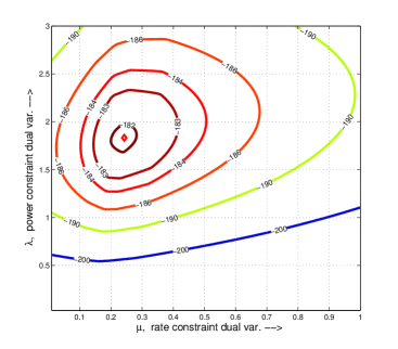
Figure 1: Contours of Dual Function, Single RT User. Parameters $N=8,K=8,M=3,\check{P}=20$ dBm, $\check{d}_{1}=50$ bps/Hz

Figure 1 shows a contour plot of the dual function $\Theta(\lambda,\boldsymbol{\mu})$ for the case of one RT user. The diamond marker shows the maximum.

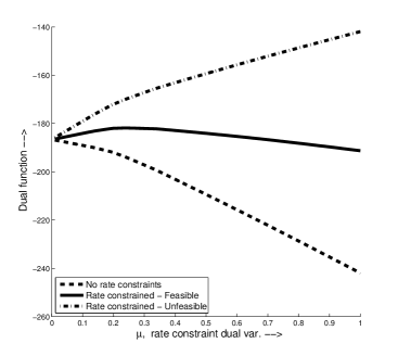
Figure 2: Dual Functions for Different Rate Constraints, $\lambda=1.83$

We can get some insight on the shape of the dual function from figure 2 where we plotted the function with respect to $\mu$ for a fixed value of $\lambda$. The solid line curve corresponds to the same dual function as in figure 1, where the rate constraint is active, $\check{d}_{1}=50$ bps/Hz. We see that the dual function goes through a maximum at $\mu=0.24$. We have also shown the case where we increase the minimum rate constraint so much that the problem becomes infeasible, e.g., we make $\check{d}_{1}=100$ bps/Hz. As expected from duality theory, the dual function has no maximum since $\lim_{\mu\rightarrow\infty}\Theta(\lambda,\boldsymbol{\mu})=\infty$ as shown by the dash-dotted curve. Finally, the dashed curve at the bottom corresponds to $\check{d}_{1}=0$ bps/Hz such that the constraint is inactive and the solution where the maximum occurs is located at $\mu_{1}=0$.

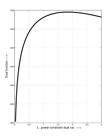
Figure 3: Dual Function vs. $\lambda$, $\mu=0.24$

For completeness we show in Figure 3 the dual function as a function of $\lambda$ when the rate constraints are feasible. The dual function increases rapidly and reaches a maximum at $\lambda=1.83$.

3.6 Dual-Based Primal Feasible Method

The SDMA set selection and beamforming vectors found by Algorithm 1 do not always provide a primal feasible solution. The rate or power constraints might be violated whenever the algorithm stops because the number of iterations has been reached before the convergence rule is met. In this subsection, we propose a simple procedure to obtain a feasible point to problem (9–15) from the dual solution found with Algorithm 1. This point is not optimal but because we start from the dual optimal solution, we expect that it will be close to the optimal solution. Obviously this will give us a lower bound to the optimal primal solution.

   Solve the dual problem (18) using algorithm 1. This yields the optimal dual variables $\lambda^{*},\boldsymbol{\mu}_{k}^{*}$ and a SDMA set assignment vector ${s}^{*}(n)$ for each subchannel $n$.

   Set $s^{o}_{0}(n)=s^{*}(n)$

  Evaluate total power and user rate constraints (10–11)

  if All constraints are met then

      Exit. A feasible solution has been found.

  end if

  Compute power allocation problem for $s^{o}_{0}(n)$ and evaluate total power and user rate constraints (10–11)

  if All constraints are met then

      Exit. A feasible solution has been found.

  end if

  Compute the multipliers $\mu_{k}$ for users $k$ such that $r_{k}<\check{d}_{k}$

  for  $j=1$ to $\overline{J}$  do

      $\mu_{k}=\mu_{k}+\delta$

      Find $s^{o}_{j}=\hbox{arg\ }\min_{s}\{f_{n,s}\}$ where $f_{n,s}$ is given by (25) for the current dual variables $\lambda,\boldsymbol{\mu}$

      Let $s^{o}_{j}(n)$ be the SDMA assignment found

     if  $s^{o}_{j}(n)\not=s^{o}_{j-1}(n)$ then

         We have found a new SDMA assignment

        Compute power allocation problem for $s^{o}_{j}(n)$ and evaluate total power and user rate constraints (10–11)

        if All constraints are met then

            Exit. A feasible solution has been found.

        end if

     end if

  end for

   Exit. A feasible solution was not found.

Algorithm 2 Calculating a Feasible Point from the Dual Solution

Algorithm 2 summarizes this method. The algorithm begins by solving the dual problem (18) using Algorithm 1. If the solution is not feasible either directly or by recomputing the power allocation for the SDMA set assignment found in the dual problem, the algorithm performs a search by increasing the dual variables associated to the users whose QoS constraints are not met until a new SDMA set assignment is found. It then solves the power allocation problem for this new SDMA set assignment and checks if the minimum rate constraints are met. The search for new SDMA sets continues using this method until a feasible SDMA set assignment is found or a maximum number of iteration is reached.

Algorithm 2 invokes algorithm 1 which has complexity $O(NK^{M}M^{3})$. Assuming that the maximum number of iterations $I_{M}$ is fixed independently of the problem parameters, the computational complexity of the feasible point search is $O(NK^{M})$ for the subcarrier reassignment and $O(N(D+K))$ for the power allocation. These are lower than the computational complexity of algorithm  1. Therefore, the computational complexity of algorithm 2 is also $O(NK^{M}M^{3})$.

In contrast to the enumeration method described in Section 2.3 which performs an enumeration of all possible SDMA set assignments, the dual-based Algorithm 2 is a method that finds new candidate SDMA set assignments close to the dual optimal and then uses them to solve a simple power allocation problem until the rate and power constraints are met. This makes the search for a near-optimal feasible point much faster than finding the exact solution.

4 Performance Analysis

In this section, we present some numerical results on the performance of the dual-based algorithm and the accuracy of the upper and lower bounds. To show how they can be used to evaluate heuristic algorithms, we also compare them with the solution provided by a weight adjustment method described in Section 4.2.

4.1 Convergence of the Dual Algorithm

First we present in Figure 4 the value of the dual function and Lagrange multipliers as a function of the number of iterations for a given channel realization. The corresponding transmit power and the rate received by the RT user are shown in Figure 5. The parameters used for the calculation are listed in the figure titles.

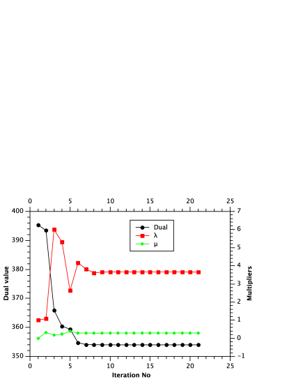
Figure 4: Dual function and multipliers for $M=3$, $K=16$, $N=16$, $\check{P}=20$ dBm, $D=1$ and $\check{d}_{1}=$80 bps/Hz.

Figure 5: Power and rate constraints for $M=3$, $K=16$, $N=16$, $\check{P}=20$ dBm, $D=1$ and $\check{d}_{1}=80$ bps/Hz.

We see that the algorithm converges very quickly to a solution that is both close to the minimum value and feasible. This is typical of several other configurations, except that the number of iteration increases with the number of RT users.

4.2 Weight Adjustment Heuristic

As discussed in Section 1.1, several RA algorithms provide support for users with RT traffic by increasing the user weights in the utility function until they receive enough transmission resources. In this section, we describe a generic weight adjustment method which will be used to show that this technique leaves much room for improvement.

  Solve RA problem (9–15) without minimum rate constraints constraints (11)

   ${\mathbf{c}}^{\prime}\leftarrow{\mathbf{c}}$

   Let $r_{k}$ be the achieved rate for user $k$ at every iteration

   iteration $\leftarrow$ 1

  while  ($r_{k}<\check{d}_{k}$ for one or more users $k\in{\mathcal{D}}$) AND (iteration $\leq\bar{I}$)  do

     Increase user weight using $c_{k}^{\prime}=c_{k}^{\prime}+\epsilon\left(\check{d}_{k}-r_{k}\right)$ for users in need, where $0<\epsilon\leq 1$

      Solve RA problem (9–15) without minimum rate constraints (11) using user weights ${\mathbf{c}}^{\prime}$

      iteration $\leftarrow$ iteration $+1$

  end while

Algorithm 3 Weight Adjustment Algorithm

We want to find a set of weights in the utility function (9) such that the rate requirements of the RT users are met when we solve problem (9–15) without the rate constraints (11). Also, the set of weights must not be very different from one user to the other in order to maximize the multi-user diversity gain. Algorithm 3 implements a generic method that can do this. It increases the user weights for RT users until enough resources are allocated to meet the minimum rate requirements. The parameter $\epsilon$ controls how much the weights are increased with respect to the rate bounds. The rates achieved by Algorithms 3 and 2 are different since they solve different problems. Algorithm 3 can be seen as solving problem (9–15) by using a linear penalty method for constraints (11) of the form

$$P_{k}=\min\left\{0,r_{k}-\check{d}_{k}\right\}.$$

The modified objective function is then

$$U_{P} =\sum_{k}c_{k}r_{k}+P_{k}$$

$$=\sum_{k}c_{k}r_{k}+\epsilon\sum_{k|r_{k}<\check{d}}(r_{k}-\check{d}).$$ (40)

At each iteration of the penalty method, whenever rate constraints are active, the solution of (40) cannot be smaller than that of (9–15) since it is a relaxation. Notice that problem (40) is quite simple since it has a single constraint for the transmit power but it has to be solved many times to adjust the weights of the real time users. In weight adjustment algorithms such as huang08 , the user weights are increased at each time slot using an increasing function of the packets delay, so the computation task is distributed over time. However, this distributed approach does not guarantee that the rate requirements are met in a given time slot which can lead to delay violations and jitter.

4.3 Parameter Setup and Methodology

We now present the method and parameter values used to compare the performance of the different methods to solve problem (9). We used a Rayleigh fading model to generate the user channels such that each component of the channel vectors ${\mathbf{h}}_{k,n}$ are i.i.d. random variables distributed as $\mathcal{CN}(0,1)$. We also assumed independent fading between users, antennas and subcarriers. Unless otherwise noted, we used a configuration with $M=3$ antennas, $K=16$ users and $N=16$ subcarriers. We have only one RT user when we examine the effect of various parameters and we also look at the impact of increasing the number of RT users. The minimum rate constraint was set at $40$ bps/Hz unless otherwise stated. We also fixed the power constraint to $\check{P}=20$ dBm and used a large-scale attenuation of 0 dB for all users. The user weights in (9) were set to $c_{k}=1$ for all users. The results are the average over the feasible cases from 100 independent channel realizations.

We compared the performance of the different methods for various scenarios where we increased the resource requirements for the RT users until the minimum rate requirements can no longer be met for all RT users. For each scenario and channel realization, the upper bound was computed from the dual solution using Algorithm 1 described in Section 3.4. For small systems, we also found the exact solution using the primal enumeration method given in Section 2.3. We also computed the lower bound given by dual-based primal feasible Algorithm 2 and the heuristic solution provided by the weight adjustment Algorithm 3 described in Section 3.6 and 4.2. We use the upper bound given by the dual optimal solution as the reference point when computing the gap when the exact solution is not available.

4.4 Single User, Increasing Minimum Rate

Method	Minimum rate (bps/Hz)
	$13.33$	$16.66$	$20$
Dual-based upper bound (bps/Hz)	49.13	47.12	40.8
Primal enum. gap (%)	0.57	0.55	0.10
Dual-based feas. gap (%)	0.57	0.59	0.04
Weight mod. gap (%)	0.68	0.71	0.15

Table 1: Average performance gap against the dual optimal upper bound for small system configuration.

In this first scenario, we have a single RT user and we increase its minimum rate $\check{d}_{1}$. First we consider a small system with $K=4$ users and $N=2$ subcarriers where it is possible to compute an exact solution. We present in table 1 the average gap in percent between the three methods used to find feasible solutions against the dual upper bound for a small system. As the required minimum rate increases from 13.33 to 20 bps/Hz, the upper bound decreases as more resources need to be assigned to the RT user until the problem is no longer feasible. For this small configuration, we see that all methods give excellent results and the duality gap is very small.

Method	Minimum rate (bps/Hz)
	80	100	120
Total rate gap against the upper bound (%)
Dual-based feas.	0.24	0.23	0.21
Weight mod.	9.49	7.30	3.36

Table 2: Average total rate gap as a function minimum rate requirement.

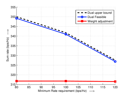
Figure 6: Average total rate as a function of the minimum rate requirements

In the remaining results, we use a larger system with $K=16$ users and $N=16$ subcarriers. With these values, it is no longer possible to use the primal enumeration method and we compute the gap relative to the dual upper bound. We present in Table 2 the difference in percentage between the bound and the solutions of the dual feasible and the weight adjustment algorithms. The dual feasible algorithm gives a lower bound within 0.25% of the dual upper bound while the weight adjustment solutions difference can be almost 10%. As discussed in Section 4.2, this is due to the fact that the weight adjustment algorithm stops as soon as it finds a feasible solution and does not have the option of finding a better assignment. As a result, the objective does not change much when the minimum rate is increased. This can be seen from Figure 6 which shows the sum rate achieved by the dual feasible algorithm and the weight modification method against the minimum rate requirement.

4.5 Single User, Increasing Attenuation

As the user moves away from the BS and the channel attenuation increases, the RA algorithm dedicates more resources to the RT user until the problem is unfeasible. Figure 7 shows the average total rate when the large-scale channel attenuation of the RT user varies from 0 to 15 dB. The results show that for all SNR, the dual lower bound provides a tight solution with the upper bound while the weight adjustment method shows a large performance gap. Table 3 shows the error in percentage between the objective and the upper bound. For an attenuation of 15 dB, neither method is able to find a feasible solution; the problem is feasible because the dual upper bound is around 140, but the algorithms cannot find a solution. That is, algorithm 1 for the dual upper bound finds a solution as long as the primal problem is feasible. On the other hand, algorithm 2 cannot find a solution when the solution point is close to the infeasibility region. In that case, the algorithm exits declaring that a feasible solution could not be found. Also, note that the proposed dual-based algorithms provides a near-optimal to the ZF problem (9–14) for all SNRs where a feasible solution can be found by the algorithm.

Figure 7: Average total rate as a function of RT user large-scale channel attenuation.

Method	RT user attenuation (dB)
	0	5	10
Total rate gap against the upper bound (%)
Dual-based feas.	0.16	0.70	0.82
Weight mod.	9.53	32.95	52.35

Table 3: Average total rate gap as a function of RT user large-scale channel attenuation.

Figure 7 shows average sum rates. The average is performed over the channel realizations that provide feasible points. When the attenuation of the RT user is low, most of the channel realizations produce feasible points. When it is high, some of the channel realizations do not produce feasible points and are discarded. For example, in figure 7 when the attenuation is $15$ dBs, none or very few of the channel realizations produce feasible points. Therefore, figure 7 does not show a sum rate for that point.

4.6 Increasing Number of RT Users

Finally, figure 8 shows the upper dual bound, the lower bound and the solution given by weight adjustment methods as a function of the number of RT users. Table 4 lists the performance gap against the dual bound in percentage. The dual feasible lower bound is again very close to the upper bound. Meanwhile, we can see that the performance of the weight adjustment method quickly degrades when the number of RT users increases. It cannot find feasible points with 6 or 7 RT users while the dual algorithm yields solutions for these values within $3.52\%$ of the upper bound.

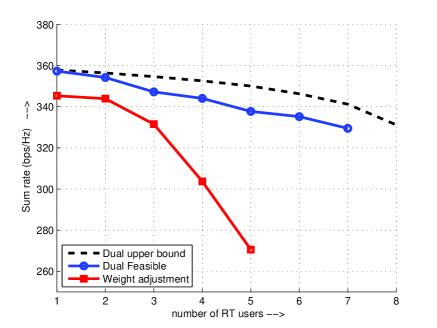
Figure 8: Average total rate as a function of the number of RT users.

Method	Number of RT users
	1	2	3	4	5	6	7
	Total rate gap against the upper bound (%)
Dual Feas.	0.16	0.61	2.09	2.41	3.52	3.20	3.43
Weight mod.	3.5	3.5	6.52	13.86	22.71	-	-

Table 4: Average total rate gap as a function of the number of RT users

For a single RT user, we have seen in tables 2 and 3 that the difference between the upper and lower solution is small. In figure 8, we see that this difference increases for three or more RT users. Still, this growth is not large and we can consider that a 3.52% is an acceptable error tolerance. Based on this, we can claim that it is possible to find a quasi-optimal solution to problem (9–15) with the proposed method, albeit with an off-line algorithm.

Furthermore, the results show that the weight modification method has a large performance gap which becomes more significant as the number of RT users increase. Also, the dual method can find feasible solutions for cases where the weight adjustment method cannot. This shows that the weight modification method should be used carefully for RA in OFDMA-SDMA systems with RT users and that more efficient heuristics should be developed to approach the performance of the dual-based feasible solution.

5 Conclusion

In this work, we proposed a method to compute the beamforming vectors and the user selection in an OFDMA-SDMA MISO system with minimum rate requirements for some RT users. We gave a rigorous mathematical formulation of the Zero-forcing model and then used a Lagrangian relaxation of the power and rate constraints to solve the dual problem using a subgradient algorithm. The Lagrange decomposition yields sub-problems separated per subcarrier, SDMA sets and users which substantially reduces the computational complexity. We obtained a simple expression of the dual function for the beamforming problem for a given SDMA set based on a pseudo-inverse condition on the beamforming vectors. The dual optimum can then be used as a benchmark to compare against any other solution methods and heuristics. The dual function also gives us a better understanding of the problem. Its shape is related to the rate constraint activation and problem feasibility, and it also justifies the splitting of the subcarrier assignment and power allocation processes used in several heuristic methods.

We then proposed an algorithm which finds a feasible point by starting from the dual-based optimum solution and searching among the dual variables of the rate constraints. Numerical results indicate that the two bounds are tight so that the feasible point is near-optimal. As a point of comparison, we also evaluated the performance of a weight adjustment method which uses weight adjustments in the objective function to achieve the required rates. Our results show that the performance gap of this approach is large and grows when the SNR of a single RT user increases or when the number of RT users increases.

In addition, the weight adjustment method requires many time slots to adjust the weights and schedule real time users. The dual-based method explicitly includes the minimum rate constraints which allows RT users to be scheduled in the current slot, which decreases the overall packet delay and jitter.

The significant gap between the weight adjustment algorithm and the optimal RA solution, suggests that there is a need to find better heuristics. The dual approach looks promising to guide the design of efficient novel heuristics. To implement the RA algorithm in real time, we also need to design fast methods to reduce the number of SDMA sets to be searched. The design of these heuristic algorithms is outside the scope of this paper and is part of our current efforts. Finally, the upper and lower bounds also provide a very useful benchmark to compare the performance of any heuristic method.

6 Abbreviations

BER

Bit Error Rate

BS

Base Station

CPU

Central Processing Unit

LTE

Long Term Evolution RA Resource Allocation

MIP

Mixed Integer Program

MISO

Multiple Input Single Output

NLP

Non Linear Program

NP

Non-deterministic Polynomial time

nRT

non Real Time

OFDMA

Orthogonal Frequency Division multiplexing Access

QoS

Quality of Service 4G Fourth Generation

RT

Real Time

SDMA

Spatial Division Multiple Access

SISO

Single Input Single Output

SNR

Signal to Noise Ratio

ZF

Zero Forcing

7 Competing interests

The authors declare that they have no competing interests.

- (1) 3GPP, “Further advancements for EUTRA: Physical layer aspects Rel. 9, 2010,” 3GPP TR 36.814 V1.2.1, Tech. Spec.n Group Radio Access Network.
- (2) IEEE, “Draft amendment to IEEE standard for local and metropolitan area networks part 16: Air interface for fixed and mobile broadband wireless access systems: Multi-hop relay specification, 2009,” Standard IEEE P802.16j/D9-2009, Institute of Electrical and Electronic Engineers.
- (3) K. Letaief and Y. Zhang, “Dynamic multiuser resource allocation and adaptation for wireless systems,” IEEE Wireless Communications Magazine, vol. 13, no. 4, pp. 38–47, Aug. 2006.
- (4) D. Bartolomé and A. Pérez-Neira, “Practical implementation of bit loading schemes for multiantenna multiuser wireless OFDM systems,” IEEE Transactions on Communications, vol. 55, no. 8, pp. 1577–1587, Aug. 2007.
- (5) T. F. Maciel and A. Klein, “A resource allocation strategy for SDMA/OFDMA systems,” in Proc. of IST Mobile and Wireless Communications Summit, Jul. 2007, pp. 1–5.
- (6) B. Ozbek and D. L. Ruyet, “Adaptive resource allocation for SDMA-OFDMA systems with genetic algorithm,” in 6th International Symposium on Wireless Communication Systems, ISWCS, Sep. 2009, pp. 483–442.
- (7) Y. Tsang and R. Cheng, “Optimal resource allocation in SDMA/multi-input-single-output/OFDM systems under QoS and power constraints,” in Proc. of WCNC, Mar. 2004, pp. 1595–1600.
- (8) P. Chan and R. Cheng, “Capacity maximization for zero-forcing MIMO-OFDMA downlink systems with multiuser diversity,” IEEE Transactions on Wireless Communications, vol. 6, no. 5, pp. 1880–1889, 2007.
- (9) L. Xingmin, T. Hui, S. Qiaoyun, and L. Lihua, “Utility based scheduling for downlink OFDMA/SDMA systems with multimedia traffic,” in Proc. IEEE Wireless Communications and Networking Conference, WCNC, Mar. 2010, pp. 130–134.
- (10) D. Perea-Vega, J. Frigon, and A. Girard, “Near-optimal and efficient heuristic algorithms for resource allocation in MISO-OFDM systems,” in IEEE International Conference on Communications ICC, May 2010, pp. 1–6.
- (11) C. Tsai, C. Chang, F. Ren, and C. Yen, “Adaptive radio resource allocation for downlink OFDMA/SDMA systems with multimedia traffic,” IEEE Transactions on Wireless Communications, vol. 7, no. 5, pp. 1734–1743, 2008.
- (12) W. Chung, L. Wang, and C. Chang, “A low-complexity beamforming-based scheduling for downlink OFDMA/SDMA systems with multimedia traffic,” in Proc. of IEEE GLOBECOM, Nov. 2009, pp. 1–5.
- (13) W. Huang, K. Sun, and T. Bo, “A new weighted proportional fair scheduling algorithm for SDMA/OFDMA systems,” in Proc. 3rd Int. Conf. on Communications and Networking in China, ChinaCom, Aug. 2008, pp. 538–541.
- (14) S. K. V. Papoutsis, I. Fraimis, “User selection and resource allocation algorithm with fairness in MISO-OFDMA,” IEEE Communications Letters, vol. 14, no. 5, pp. 411–413, 2010.
- (15) V. Papoutsis and S. Kotsopoulos, “Resource Allocation Algorithm for MISO-OFDMA Systems with QoS provisioning,” in The Seventh International Conference on Wireless and Mobile Communications, ICWMC, 2011, pp. 7–11.
- (16) V. Tralli, P. Henarejos, and A. Perez-Neira, “A low complexity scheduler for multiuser MIMO-OFDMA systems with heterogeneous traffic,” in Proc. International Conference on Information Networking, ICOIN, Jan. 2011, pp. 251–256.
- (17) X. Wang and G. Giannakis, “Ergodic capacity and average rate-guaranteed scheduling for wireless multiuser OFDM systems,” in International Symposium on Information Theory, ISIT., Jul. 2008, pp. 1691–1695.
- (18) T. Yoo and A. Goldsmith, “On the optimality of multiantenna broadcast scheduling using zero-forcing beamforming,” IEEE Journal on Selected Areas in Communications, vol. 24, no. 3, pp. 528–541, Mar. 2006.
- (19) D. Bertsekas, Convex Analysis and Optimization. Athena Scientific – Belmont, MA, 2003.
- (20) A. Wiesel, Y. Eldar, and S. Shamai, “Optimal generalized inverses for zero forcing precoding,” in Proc. of 41st Annual Conf. on Information Sciences and Systems, 2007.
- (21) Matlab. (2012, Nov.) Moore-Penrose pseudoinverse of matrix. Matlab documentation center. [Online]. Available: http://www.mathworks.com/help/matlab/ref/pinv.html
- (22) L. V. S. Boyd, Convex Optimization. Cambridge University Press, 2004.