Clustering comparison of point processes with applications to random geometric models

Abstract

In this chapter we review some examples, methods, and recent results involving comparison of clustering properties of point processes. Our approach is founded on some basic observations allowing us to consider void probabilities and moment measures as two complementary tools for capturing clustering phenomena in point processes. As might be expected, smaller values of these characteristics indicate less clustering. Also, various global and local functionals of random geometric models driven by point processes admit more or less explicit bounds involving void probabilities and moment measures, thus aiding the study of impact of clustering of the underlying point process. When stronger tools are needed, directional convex ordering of point processes happens to be an appropriate choice, as well as the notion of (positive or negative) association, when comparison to the Poisson point process is considered. We explain the relations between these tools and provide examples of point processes admitting them. Furthermore, we sketch some recent results obtained using the aforementioned comparison tools, regarding percolation and coverage properties of the Boolean model, the SINR model, subgraph counts in random geometric graphs, and more generally, U-statistics of point processes. We also mention some results on Betti numbers for Čech and Vietoris-Rips random complexes generated by stationary point processes. A general observation is that many of the results derived previously for the Poisson point process generalise to some “sub-Poisson” processes, defined as those clustering less than the Poisson process in the sense of void probabilities and moment measures, negative association or dcx-ordering.

1 Introduction

On the one hand, various interesting methods have been developed for studying local and global functionals of geometric structures driven by Poisson or Bernoulli point processes (see MeeRoy96 ; Penrose03 ; Yukich12 ). On the other hand, as will be shown in the following section, there are many examples of interesting point processes that occur naturally in theory and applications. So, the obvious question arises how much of the theory developed for Poisson or Bernoulli point processes can be carried over to other classes of point processes.

Our approach to this question is based on the comparison of clustering properties of point processes. Roughly speaking, a set of points in $\mathbb{R}^{d}$ clusters if it lacks spatial homogeneity, i.e., one observes points forming groups which are well spaced out. Many interesting properties of random geometric models driven by point processes should depend on the “degree” of clustering. For example, it is natural to expect that concentrating points of a point process in well-spaced-out clusters should negatively impact connectivity of the corresponding random geometric (Gilbert) graph, and that spreading these clustered points “more homogeneously” in the space would result in a smaller critical radius for which the graph percolates. For many other functionals, using similar heuristic arguments one can conjecture whether increase or decrease of clustering will increase or decrease the value of the functional. However, to the best of our knowledge, there has been no systematic approach towards making these arguments rigorous.

The above observations suggest the following program. We aim at identifying a class or classes of point processes, which can be compared in the sense of clustering to a (say homogeneous) Poisson point process, and for which — by this comparison — some results known for the latter process can be extrapolated. In particular, there are point processes which in some sense cluster less (i.e. spread their points more homogeneously in the space) than the Poisson point process. We call them sub-Poisson. Furthermore, we hasten to explain that the usual strong stochastic order (i.e. coupling as a subset of the Poisson process) is in general not an appropriate tool in this context.

Various approaches to mathematical formalisation of clustering will form an important part of this chapter. By formalisation, we mean defining a partial order on the space of point processes such that being smaller with respect to the order indicates less clustering. The most simple approach consists in considering void probabilities and moment measures as two complementary tools for capturing clustering phenomena in point processes. As might be expected, smaller values of these characteristics indicate less clustering. When stronger tools are needed, directionally convex (dcx) ordering of point processes happens to be a good choice, as well as the notion of negative and positive association. Working with these tools, we first give some useful, generic inequalities regarding Laplace transforms of the compared point processes. In the case of dcx-ordering these inequalities can be generalised to dcx functions of shot-noise fields.

Having described the clustering comparison tools, we present several particular results obtained by using them. Then, in more detail, we study percolation in the Boolean model (seen as a random geometric graph) and the SINR graph. In particular, we show how the classical results regarding the existence of a non-trivial phase transition extend to models based on additive functionals of various sub-Poisson point processes. Furthermore, we briefly discuss some applications of the comparison tools to U-statistics of point processes, counts of sub-graphs and simplices in random geometric graphs and simplicial complexes, respectively. We also mention results on Betti numbers of Čech and Vietoris-Rips random complexes generated by sub-Poisson point processes.

Let us conclude the above short motivating introduction by citing an excerpt from a standard reference on stochastic comparison methods by Müller and Stoyan (2002): “It is clear that there are processes of comparable variability. Examples of such processes are a homogeneous Poisson process and a cluster process of equal intensity or two hard-core Gibbs processes of equal intensity and different hard-core distances. It would be fine if these variability differences could be characterized by order relations … [implying], for example, reasonable relationship[s] for second order characteristics such as the pair correlation function.”; cf (Muller02, , page 253). We believe that the results reported in this chapter present one of the first answers to the above call, although “Still much work has to be done in the comparison theory for point processes.” (ibid.)

The present chapter is organised as follows. In Sect. 2 we recall some examples of point processes. The idea is to provide as many as possible examples which admit various clustering comparison orders, described then in Sect. 3. An extensive overview of applications is presented in Sect. 4.

2 Examples of Point Processes

In this section we give some examples of point processes, where our goal is to present them in the context of modelling of clustering phenomena. Note that throughout this chapter, we consider point processes on the $d$-dimensional Euclidean space $\mathbb{R}^{d}$, $d\geq 1$, although much of the presented results have straightforward extensions to point processes on an arbitrary Polish space.

2.1 Elementary Models

A first example we probably think of when trying to come up with some spatially homogeneous model is a point process on a deterministic lattice.

Definition 1 (Lattice point process)

By a lattice point process $\Phi_{\mathbb{L}}$ we mean a simple point process whose points are located on the vertices of some deterministic lattice $\mathbb{L}$. An important special case is the $d$-dimensional cubic lattice $\Delta\mathbb{Z}^{d}=\{\Delta(u_{1},\ldots,u_{d}),u_{i}\in\mathbb{Z}\}$ of edge length $\Delta>0$, where $\mathbb{Z}$ denotes the set of integers. Another specific (two-dimensional) model is the hexagonal lattice on the complex plane given by $\Delta\mathbb{H}=\{\Delta(u_{1}+u_{2}e^{\emph{i}\pi/3}),\ u_{1},u_{2}\in\mathbb{Z}\}$. The stationary version $\Phi_{\mathbb{L}}^{\text{st}}$of a lattice point process $\Phi_{\mathbb{L}}$ can be constructed by randomly shifting the deterministic pattern through a vector $U$ uniformly distributed in some fixed cell of the lattice $\mathbb{L}$, i.e. $\Phi_{\mathbb{L}}^{\text{st}}=\Phi_{\mathbb{L}}+U.$ Note that the intensity of the stationary lattice point process is equal to the inverse of the cell volume. In particular, the intensity $\lambda_{\Delta\mathbb{Z}^{d}}$ of $\Phi_{\Delta\mathbb{Z}^{d}}^{\text{st}}$ is equal to $\lambda_{\Delta\mathbb{Z}^{d}}=1/\Delta^{d}$, while that of $\Phi_{\Delta\mathbb{H}}^{\text{st}}$ is equal to $\lambda_{\Delta\mathbb{H}}=2/(\sqrt{3}/\Delta^{2})$.

Lattice point processes are usually considered to model “perfect” or “ideal” structures, e.g. the hexagonal lattice on the complex plane is used to study perfect cellular communication networks. We will see however, without further modifications, they escape from the clustering comparison methods presented in Sect. 3.

When the “perfect structure” assumption cannot be retained and one needs a random pattern, then the Poisson point process usually comes as a natural first modelling assumption. We therefore recall the definition of the Poisson process for the convenience of the reader, see also the survey given in baddeley12 .

Definition 2 (Poisson point process)

Let $\Lambda$ be a (deterministic) locally finite measure on the Borel sets of $\mathbb{R}^{d}$. The random counting measure $\Pi_{\Lambda}$ is called a Poisson point process with intensity measure $\Lambda$ if for every $k=1,2,\ldots$ and all bounded, mutually disjoint Borel sets $B_{1},\allowbreak\ldots,B_{k}$, the random variables $\Pi_{\Lambda}(B_{1}),\allowbreak\ldots,\Pi_{\Lambda}(B_{k})$ are independent, with Poisson distribution ${\rm Pois}(\Lambda(B_{1})),\ldots,{\rm Pois}(\Lambda(B_{k}))$, respectively. In the case when $\Lambda$ has an integral representation $\Lambda(B)=\int_{B}\lambda(x)\,\mathrm{d}x$, where $\lambda:\mathbb{R}^{d}\rightarrow\mathbb{R}_{+}$ is some measurable function, we call $\lambda$ the intensity field of the Poisson point process. In particular, if $\lambda$ is a constant, we call $\Pi_{\Lambda}$ a homogeneous Poisson point process and denote it by $\Pi_{\lambda}$.

The Poisson point process is a good model when one does not expect any “interactions” between points. This is related to the complete randomness property of Poisson processes, cf. (DVJI2003, , Theorem 2.2.III). The homogeneous Poisson point process is commonly considered as a reference model in comparative studies of clustering phenomena.

2.2 Cluster Point Processes — Replicating and Displacing Points

We now present several operations on the points of a point process, which in conjunction with the two elementary models presented above allow us to construct various other interesting examples of point processes. We begin by recalling the following elementary operations.

Superposition of patterns of points consists of set-theoretic addition of these points. Superposition of (two or more) point processes $\Phi_{1},\ldots,\Phi_{n}$, defined as random counting measures, consists of adding these measures $\Phi_{1}+\cdots+\Phi_{n}$. Superposition of independent point processes is of special interest.

Thinning of a point process consists of suppressing some subset of its points. Independent thinning with retention function $p(x)$ defined on $\mathbb{R}^{d}$, $0\leq p(x)\leq 1$, consists in suppressing points independently, given a realisation of the point process, with probability $1-p(x)$, which might depend on the location $x$ of the point to be suppressed or not.

Displacement consists in, possibly randomised, mapping of points of a point process to the same or another space. Independent displacement with displacement (probability) kernel $\mathcal{X}(x,\cdot)$ from $\mathbb{R}^{d}$ to $\mathbb{R}^{d^{\prime}}$, $d^{\prime}>1$, consists of independently mapping each point $x$ of a given realisation of the original point process to a new, random location in $\mathbb{R}^{d^{\prime}}$ selected according to the kernel $\mathcal{X}(x,\cdot)$.

Remark 1

An interesting property of the class of Poisson point processes is that it is closed with respect to independent displacement, thinning and superposition, i.e. the result of these operations made on Poisson point processes is a Poisson point process, which is not granted in the case of an arbitrary (i.e. not independent) superposition or displacement, see e.g. DVJI2003 ; DVJII2007 .

Now, we define a more sophisticated operation on point processes that will allow us to construct new classes of point processes with interesting clustering properties.

Definition 3 (Clustering perturbation of a point process)

Let $\Phi$ be a point process on $\mathbb{R}^{d}$ and $\mathcal{N}(\cdot,\cdot)$, $\mathcal{X}(\cdot,\cdot)$ be two probability kernels from $\mathbb{R}^{d}$ to the set of non-negative integers $\mathbb{Z}_{+}$ and $\mathbb{R}^{d^{\prime}}$, $d,d^{\prime}\geq 1$, respectively. Consider the following subset of $\mathbb{R}^{d^{\prime}}$. Let

$$\Phi^{\text{pert}}=\bigcup_{X\in\Phi}\bigcup_{i=1}^{N_{X}}\{Y_{iX}\}\,,$$ (1)

where, given $\Phi$,

• $(N_{X})_{X\in\Phi}$ are independent, non-negative integer-valued random variables with (conditional) distribution $\mathbf{P}\left(N_{X}\in\cdot\,|\,\Phi\right)=\mathcal{N}(X,\cdot)$,

• ${Y}_{X}=(Y_{iX};i=1,2,\ldots)$, $X\in\Phi$ are independent vectors of i.i.d. random elements of $\mathbb{R}^{d^{\prime}}$, with $Y_{iX}$ having the conditional distribution $\mathbf{P}\left(Y_{iX}\in\cdot\,|\,\Phi\right)=\mathcal{X}(X,\cdot)$.

Note that the inner sum in (1) is interpreted as $\emptyset$ when $N_{X}=0$.

The random set $\Phi^{\text{pert}}$ given in (1) can be considered as a point process on $\mathbb{R}^{d^{\prime}}$ provided it is a locally finite. In what follows, we will assume a stronger condition, namely that the itensity measure of $\Phi^{\text{pert}}$ is locally finite (Radon), i.e.

$$\int_{\mathbb{R}^{d}}n(x)\mathcal{X}(x,B)\,\alpha(\mathrm{d}x)<\infty,$$ (2)

for all bounded Borel sets $B\subset\mathbb{R}^{d^{\prime}}$, where $\alpha(\cdot)=\mathbf{E}\left(\Phi\right)(\cdot)$ denotes the intensity measure of $\Phi$ and

$$n(x)=\sum_{k=1}^{\infty}k\mathcal{N}(x,\{k\})$$ (3)

is the mean value of the distribution $\mathcal{N}(x,\cdot)$.

Clustering perturbation of a given parent process $\Phi$ consists in independent replication and displacement of the points of $\Phi$, with the number of replications of a given point $X\in\Phi$ having distribution $\mathcal{N}(X,\cdot)$ and the replicas’ locations having distribution $\mathcal{X}(X,\cdot)$. The replicas of $X$ form a cluster.

For obvious reasons, we call $\Phi^{\text{pert}}$ a perturbation of $\Phi$ driven by the replication kernel $\mathcal{N}$ and the displacement kernel $\mathcal{X}$. It is easy to see that the independent thinning and displacement operations described above are special cases of clustering perturbation. In what follows we present a few known examples of point processes arising as clustering perturbations of a lattice or Poisson point process. For simplicity we assume that replicas stay in the same state space, i.e. $d=d^{\prime}$.

Example 1 (Binomial point process)

A (finite) binomial point process has a fixed total number $n<\infty$ of points, which are independent and identically distributed according to some (probability) measure $\Lambda$ on $\mathbb{R}^{d}$. It can be seen as a Poisson point process $\Pi_{n\Lambda}$ conditioned to have $n$ points, cf. DVJI2003 . Note that this property might be seen as a clustering perturbation of a one-point process, with deterministic number $n$ of point replicas and displacement distribution $\Lambda$.

Example 2 (Bernoulli lattice)

The Bernoulli lattice arises as independent thinning of a lattice point process; i.e., each point of the lattice is retained (but not displaced) with some probability $p\in(0,1)$ and suppressed otherwise.

Example 3 (Voronoi-perturbed lattices)

These are perturbed lattices with displacement kernel $\mathcal{X}$, where the distribution $\mathcal{X}(x,\cdot)$ is supported on the Voronoi cell $\mathcal{V}(x)$ of vertex $x\in\mathbb{L}$ of the original (unperturbed) lattice $\mathbb{L}$. In other words, each replica of a given lattice point gets independently translated to some random location chosen in the Voronoi cell of the original lattice point. Note that one can also choose other bijective, lattice-translation invariant mappings of associating lattice cells to lattice points; e.g. associate a given cell of the square lattice on the plane $\mathbb{R}^{2}$ to its “south-west” corner.

By a simple perturbed lattice we mean the Voronoi-perturbed lattice whose points are uniformly translated in the corresponding cells, without being replicated. Interestingly enough, the Poisson point process $\Pi_{\Lambda}$ with some intensity measure $\Lambda$ can be constructed as a Voronoi-perturbed lattice. Indeed, it is enough to take the Poisson replication kernel $\mathcal{N}$ given by $\mathcal{N}(x,\cdot)={\rm Pois}(\Lambda(\mathcal{V}(x)))$ and the displacement kernel $\mathcal{X}$ with $\mathcal{X}(x,\cdot)=\Lambda(\cdot\cap\mathcal{V}(x))/\Lambda(\mathcal{V}(x))$; cf. Exercise 1. Keeping the above displacement kernel and replacing the Poisson distribution in the replication kernel by some other distributions convexly smaller or larger than the Poisson distribution, one gets the following two particular classes of Voronoi-perturbed lattices, clustering their points less or more than the Poisson point process $\Pi_{\Lambda}$ (in a sense that will be formalised in Sect. 3).

Sub-Poisson Voronoi-perturbed lattices are Voronoi-perturbed lattices such that $\mathcal{N}(x,\cdot)$ is convexly smaller than ${\rm Pois}(\Lambda(\mathcal{V}(x)))$. Examples of distributions convexly smaller than ${\rm Pois}(\lambda)$ are the hyper-geometric distributions $\mathrm{HGeo}(n,m,k)$, $m,k\leq n$, $km/n=\lambda$ and the binomial distributions. ${\rm Binom}(n,\lambda/n)$, $\lambda\leq n$, which can be ordered as follows:

$$\mathrm{HGeo}(n,m,\lambda n/m)\leq_{\text{cx}}{\rm Binom}(m,\lambda/m)\leq_{\text{cx}}{\rm Binom}(r,\lambda/r)\leq_{\text{cx}}{\rm Pois}(\lambda),$$ (4)

for $\lambda\leq m\leq\min(r,n)$; cf. Whitt1985 . Recall that ${\rm Binom}(n,p)$ has the probability mass function $p_{{\rm Binom}(n,p)}(i)={n\choose i}p^{i}(1-p)^{n-i}$ ($i=0,\ldots,n$), whereas $\mathrm{HGeo}(n,m,k)$ has the probability mass function $p_{\mathrm{HGeo}(n,m,k)}(i)={m\choose i}{n-m\choose k-i}/{n\choose k}$ ($\max(k-n+m,0)\leq i\leq m$); cf. Exercise 2.

Super-Poisson Voronoi-perturbed lattices are Voronoi-perturbed lattices with $\mathcal{N}(x,\cdot)$ convexly larger than ${\rm Pois}(\Lambda(\mathcal{V}(x)))$. Examples of distributions convexly larger than ${\rm Pois}(\lambda)$ are the negative binomial distribution ${\mathrm{NBionom}}(r,p)$ with $rp/(1-p)=\lambda$ and the geometric distribution $\mathrm{Geo}(p)$ distribution $1/p-1=\lambda$, which can be ordered in the following way:

$${\rm Pois}(\lambda) \leq_{\text{cx}} \mathrm{NBionom}(r_{2},\lambda/(r_{2}+\lambda))\leq_{\text{cx}}\mathrm{NBionom}(r_{1},\lambda/(r_{1}+\lambda))$$ (5)

$$\leq_{\text{cx}} \mathrm{Geo}(1/(1+\lambda))\leq_{\text{cx}}\sum_{j}\lambda_{j}\;\mathrm{Geo}(p_{j})$$

with $r_{1}\leq r_{2}$, $0\leq\lambda_{j}\leq 1$, $\sum_{j}\lambda_{j}=1$ and $\sum_{j}\lambda_{j}/p_{j}=\lambda+1$, where the largest distribution in (5) is a mixture of geometric distributions having mean $\lambda$. Note that any mixture of Poisson distributions having mean $\lambda$ is in cx-order larger than ${\rm Pois}(\lambda)$. Furthermore, recall that the probability mass functions of $\mathrm{Geo}(p)$ and $\mathrm{NBionom}(r,p)$ are given by $p_{\mathrm{Geo}(p)}(i)=p(1-p)^{i}$ and $p_{\mathrm{NBionom}(r,p)}(i)={r+i-1\choose i}p^{i}(1-p)^{r}$, respectively.

Example 4 (Generalised shot-noise Cox point processes)

These are clustering perturbations of an arbitrary parent point process $\Phi$, with replication kernel $\mathcal{N}$, where $\mathcal{N}(x,\cdot)$ is the Poisson distribution ${\rm Pois}(n(x))$ and $n(x)$ is the mean value given in (3). Note that in this case, given $\Phi$, the clusters (i.e. replicas of the given parent point) form independent Poisson point process $\Pi_{n(X)\mathcal{X}(X,\cdot)}$, $X\in\Phi$. This special class of Cox point processes (cf. Sect. 2.3) has been introduced in Moller05 .

Example 5 (Poisson-Poisson cluster point processes)

This is a special case of the generalised shot-noise Cox point processes, with the parent point process being Poisson, i.e. $\Phi=\Pi_{\Lambda}$ for some intensity measure $\Lambda$. A further special case is often discussed in the literature, where the displacement kernel $\mathcal{X}$ is such that $\mathcal{X}(X,\cdot)$ is the uniform distribution in the ball $B_{r}(X)$ of some given radius $r$. It is called the Matérn cluster point process. If $\mathcal{X}(X,\cdot)$ is symmetric Gaussian, then the resulting Poisson-Poisson cluster point process is called a (modified) Thomas point process.

Example 6 (Neyman-Scott point process)

These point processes arise as a clustering perturbation of a Poisson parent point process $\Pi_{\Lambda}$, with arbitrary (not necessarily Poisson) replication kernel $\mathcal{N}$.

2.3 Cox Point Processes— Mixing Poisson Distributions

We now consider a rich class of point processes known also as doubly stochastic Poisson point process, which are often used to model patterns exhibiting more clustering than the Poisson point process.

Definition 4 (Cox point process)

Let $\mathfrak{L}$ be a random locally finite (non-null) measure on $\mathbb{R}^{d}$. A Cox point process $Cox_{\mathfrak{L}}$ on $\mathbb{R}^{d}$ generated by $\mathfrak{L}$ is defined as point process having the property that $Cox_{\mathfrak{L}}$ conditioned on $\mathfrak{L}=\Lambda$ is the Poisson point process $\Pi_{\Lambda}$. Note that $\mathfrak{L}$ is called the random intensity measure of $Cox_{\mathfrak{L}}$. In case when the random measure $\mathfrak{L}$ has an integral representation $\mathfrak{L}(B)=\int_{B}\xi(x)\,\mathrm{d}x$, with $\{\xi(x),x\in\mathbb{R}^{d}\}$ being a random field, we call this field the random intensity field of the Cox process. In the special case that $\xi(x)=\xi\lambda(x)$ for all $x\in\mathbb{R}^{d}$, where $\xi$ is a (non-negative) random variable and $\lambda$ a (non-negative) deterministic function, the corresponding Cox point process is called a mixed Poisson point process.

Cox processes may be seen as a result of an operation transforming some random measure $\mathfrak{L}$ into a point process $Cox_{\mathfrak{L}}$, being a mixture of Poisson processes.

In Sect. 2.2, we have already seen that clustering perturbation of an arbitrary point process with Poisson replication kernel gives rise to Cox processes (cf. Example 4), where Poisson-Poisson cluster point processes are special cases with Poisson parent point process. This latter class of point processes can be naturally extended by replacing the Poisson parent process by a Lévy basis.

Definition 5 (Lévy basis)

A collection of real-valued random variables $\{Z(B),B\in\mathcal{B}_{0}\}$, where $\mathcal{B}_{0}$ denotes the family of bounded Borel sets in $\mathbb{R}^{d}$, is said to be a Lévy basis if the $Z(B)$ are infinitely divisible random variables and for any sequence $\{B_{n}\}$, $n\geq 1$, of disjoint bounded Borel sets in $\mathbb{R}^{d}$, $Z(B_{1}),Z(B_{2}),\ldots$ are independent random variables (complete independence property), with $Z(\bigcup_{n}B_{n})=\sum_{n}Z(B_{n})$ almost surely provided that $\bigcup_{n}B_{n}$ is bounded.

In this chapter, we shall consider only non-negative Lévy bases. We immediately see that the Poisson point process is a special case of a Lévy basis. Many other concrete examples of Lévy bases can be obtained by “attaching” independent, infinitely divisible random variables $\xi_{i}$ to a deterministic, locally finite sequence $\{x_{i}\}$ of (fixed) points in $\mathbb{R}^{d}$ and letting $Z(B)=\sum_{i}\xi_{i}\mathbf{1}(x_{i}\in B)$. In particular, clustering perturbations of a lattice, with infinitely divisible replication kernel and no displacement (i.e. $\mathcal{X}(x,\cdot)=\delta_{x}$, where $\delta_{x}$ is the Dirac measure at $x$) are Lévy bases. Recall that any degenerate (deterministic), Poisson, negative binomial, gamma as well as Gaussian, Cauchy, Student’s distribution are examples of infinitely divisible distributions.

It is possible to define an integral of a measurable function with respect to a Lévy basis (even if the latter is not always a random measure; see Hellmund08 for details) and consequently consider the following classes of Cox point processes.

Example 7 (Lévy-based Cox point process)

Consider a Cox point process $Cox_{\mathfrak{L}}$ with random intensity field that is an integral shot-noise field of a Lévy basis, i.e. $\xi(y)=\int_{\mathbb{R}^{d}}k(x,y)\allowbreak Z(\mathrm{d}x)$, where $Z$ is a Lévy basis and $k:\mathbb{R}^{d}\times\mathbb{R}^{d}\rightarrow\mathbb{R}_{+}$ is some non-negative function almost surely integrable with respect to $Z\otimes\mathrm{d}y$.

Example 8 (Log-Lévy-based Cox point process)

These are Cox point processes with random intensity field given by $\xi(y)=\exp\left(\int_{\mathbb{R}^{d}}k(x,y)Z(\mathrm{d}x)\right)$, where $Z$ and $k$ satisfy the same conditions as above.

Both Lévy- and log-Lévy-based Cox point processes have been introduced in Hellmund08 , where one can find many examples of these processes. We still mention another class of Cox point processes considered in Moller98 .

Example 9 (Log-Gaussian Cox point process)

Consider a Cox point process whose random intensity field is given by $\xi(y)=\exp\left(\eta(y)\right)$ where $\{\eta(y)\}$ is a Gaussian random field.

2.4 Gibbs and Hard-Core Point Processes

Gibbs and hard-core point processes are two further classes of point processes, which should appear in the context of modelling of clustering phenomena.

Roughly speaking Gibbs point processes are point processes having a density with respect to the Poisson point process. In other words, we obtain a Gibbs point process, when we “filter” Poisson patterns of points, giving more chance to appear for some configurations and less chance (or completely suppressing) some others. A very simple example is a Poisson point process conditioned to obey some constraint regarding its points in some bounded Borel set (e.g. to have some given number of points there). Depending on the “filtering” condition we may naturally create point processes which cluster more or less than the Poisson point process.

Hard-core point processes are point process in which the points are separated from each other by some minimal distance, hence in some sense clustering is “forbidden by definition”.

However, we will not give precise definitions, nor present particular examples from these classes of point processes, because, unfortunately, we do not have yet interesting enough comparison results for them, to be presented in the remaining part of this chapter.

2.5 Determinantal and Permanental Point Process

We briefly recall two special classes of point processes arising in random matrix theory, combinatorics, and physics. They are “known” to cluster their points, less or more, respectively, than the Poisson point process.

Definition 6 (Determinantal point process)

A simple point process on $\mathbb{R}^{d}$ is said to be a determinantal point process with a kernel function $k:\mathbb{R}^{d}\times\mathbb{R}^{d}\rightarrow\mathbb{C}$ with respect to a Radon measure $\mu$ on $\mathbb{R}^{d}$ if the joint intensities $\rho^{(\ell)}$ of the factorial moment measures of the point process with respect to the product measure $\mu^{\otimes\ell}$ satisfy $\rho^{(\ell)}(x_{1},\ldots,x_{\ell})=\det\big{(}k(x_{i},x_{j})\big{)}_{1\leq i,j\leq\ell}$ for all $\ell$, where $\big{(}a_{ij}\big{)}_{1\leq i,j\leq\ell}$ stands for a matrix with entries $a_{ij}$ and $\det$ denotes the determinant of the matrix.

Definition 7 (Permanental point process)

Similar to the notion of a determinantal point process, one says that a simple point process is a permanental point process with a kernel function $k:\mathbb{R}^{d}\times\mathbb{R}^{d}\rightarrow\mathbb{C}$ with respect to a Radon measure $\mu$ on $\mathbb{R}^{d}$ if the joint intensities $\rho^{(\ell)}$ of the point process with respect to $\mu^{\otimes\ell}$ satisfy $\rho^{(\ell)}(x_{1},\ldots,x_{\ell})=\text{per}\big{(}k(x_{i},x_{j})\big{)}_{1\leq i,j\leq\ell}$ for all $\ell$, where $\text{per}\big{(}\cdot\big{)}$ stands for the permanent of a matrix. From (Ben06, , Proposition 35 and Remark 36), we know that each permanental point process is a Cox point process.

Naturally, the kernel function $k$ needs to satisfy some additional assumptions for the existence of the point processes defined above. We refer to (Ben09, , Chap. 4) for a general framework which allows to study determinantal and permanental point processes, see also Ben06 . Regarding statistical aspects and simulation methods for determinantal point processes, see Lavancier12 .

Here is an important example of a determinantal point process recently studied on the theoretical ground (cf. e.g. Goldman2010 ) and considered in modelling applications (cf. Miyoshi2012 ).

Example 10 (Ginibre point process)

This is the determinantal point process on $\mathbb{R}^{2}$ with kernel function $k((x_{1},x_{2}),\allowbreak(y_{1},y_{2}))=\exp[(x_{1}y_{1}+x_{2}y_{2})+i(x_{2}y_{1}-x_{1}y_{2})]$, $x_{j},y_{j}\in\mathbb{R}$, $j=1,2$, with respect to the measure $\mu(\mathrm{d}(x_{1},x_{2}))=\pi^{-1}\exp[-x_{1}^{2}-x_{2}^{2}]\,\mathrm{d}x_{1}\mathrm{d}x_{2}$.

Exercise 1

Let $\Phi$ be a simple point process on $\mathbb{R}^{d}$. Consider its cluster perturbation $\Phi^{\text{pert}}$ defined in (1) with the Poisson replication kernel $\mathcal{N}(x,\cdot)={\rm Pois}(\Lambda(\mathcal{V}(x)))$, where $\mathcal{V}(x)$ is the Voronoi cell of $x$ in $\Phi$, and the displacement kernel $\mathcal{X}(x,\cdot)=\Lambda(\cdot\cap\mathcal{V}(x))/\Lambda(\mathcal{V}(x))$, for some given deterministic Radon measure $\Lambda$ on $\mathbb{R}^{d}$. Show that $\Phi^{\text{pert}}$ is Poisson with intensity measure $\Lambda$.

Exercise 2

Prove (4) and (5) by showing the logarithmic concavity of the ratio of the respective probability mass functions, which implies increasing convex order and, consequently, cx-order provided the distributions have the same means.

3 Clustering Comparison Methods

Let us begin with the following informal definitions. A set of points is spatially homogeneous if approximately the same numbers of points occur in any spherical region of a given volume. A set of points clusters if it lacks spatial homogeneity; more precisely, if one observes points arranged in groups being well spaced out.

Looking at Fig. 1, it is intuitively obvious that (realisations of) some point processes cluster less than others. However, the mathematical formalisation of such a statement appears not so easy. In what follows, we present a few possible approaches. We begin with the usual statistical descriptors of spatial homogeneity, then show how void probabilities and moment measures come into the picture, in particular in relation to another notion useful in this context: positive and negative association. Finally we deal with directionally convex ordering of point processes.

This kind of organisation roughly corresponds to presenting ordering methods from weaker to stronger ones; cf. Fig. 2. We also show how the different examples presented in Sect. 2 admit these comparison methods, mentioning the respective results in their strongest versions. We recapitulate results regarding comparison to the Poisson process in Fig. 3.

simple perturbed lattice

Poisson point process

Cox point process

Fig. 1: From left to right : patterns sampled from a simple perturbed lattice (cf. Example 3), Poisson point process and a doubly stochastic Poisson (Cox) point process, all with the same mean number of points per unit area.

3.1 Second-order statistics

In this section we restrict ourselves to the stationary setting.

Ripley’s K-Function

One of the most popular functions for the statistical analysis of spatial homogeneity is Ripley’s K-function $K:\mathbb{R}_{+}\rightarrow\mathbb{R}_{+}$ defined for stationary point processes (cf. stoyetal95 ). Assume that $\Phi$ is a stationary point process on $\mathbb{R}^{d}$ with finite intensity $\lambda=\mathbf{E}{\Phi([0,1]^{d})}$. Then

$$K(r)=\frac{1}{\lambda\nu_{d}(B)}\mathbf{E}\left(\sum\right)_{X_{i}\in\Phi\cap B}(\Phi(B_{X_{i}}(r))-1)\,,$$

where $\nu_{d}(B)$ denotes the Lebesgue measure of a bounded Borel set $B\subset\mathbb{R}^{d}$, assuming that $\nu_{d}(B)>0$. Due to stationarity, the definition does not depend on the choice of $B$.

The value of $\lambda K(r)$ can be interpreted as the average number of “extra” points observed within the distance $r$ from a randomly chosen (so-called typical) point. Campbell’s formula from Palm theory of stationary point processes gives a precise meaning to this statement. Consequently, for a given intensity $\lambda$, the more one finds points of a point process located in clusters of radius $r$, the larger the value of $K(r)$ is, whence a first clustering comparison method follows. Larger values $K(r)$ of Ripley’s K-function indicate more clustering “at the cluster-radius scale” $r$. For the (homogeneous) Poisson process $\Pi_{\lambda}$ on $\mathbb{R}^{d}$, which is often considered as a “reference model” for clustering, we have $K(r)=\kappa_{d}r^{d}$, where $\kappa_{d}$ is the volume of the unit ball in $\mathbb{R}^{d}$. Note here that $K(r)$ describes clustering characteristics of the point process at the (cluster radius) scale $r$. Many point processes, which we tend to think that they cluster less or more than the Poisson point process, in fact are not comparable in the sense of Ripley’s K-function (with the given inequality holding for all $r\geq 0$, neither, in consequence, in any stronger sense considered later in this section), as we can see in the following simple example.

The following result of D. Stoyan from 1983 can be considered as a precursor to our theory of clustering comparison. It says that the convex ordering of Ripley’s K-functions implies ordering of variances of number of observed points. We shall see in Remark 2 that variance bounds give us simple concentration inequalities for the distribution of the number of observed points. These inequalities help to control clustering. We will develop this idea further in Section 3.2 and 3.3 showing that using moment measures and void probabilities one can obtain stronger, exponential concentration equalities.

Proposition 1 ((Stoyan1983inequalities, , Corollary 1))

Consider two stationary, isotropic point processes $\Phi_{1}$ and $\Phi_{2}$ of the same intensity, with the Ripley’s functions $K_{1}$ and $K_{2}$, respectively. If $K_{1}\leq_{dc}K_{2}$ i.e., $\int_{0}^{\infty}f(r)K_{1}(\mathrm{d}r)\leq\int_{0}^{\infty}f(r)K_{2}(\mathrm{d}r)$ for all decreasing convex $f$ then $\mathbf{v}\mathbf{a}\mathbf{r}(\Phi_{1}(B))\leq\mathbf{v}\mathbf{a}\mathbf{r}(\Phi_{2}(B))$ for all compact, convex $B$.

Exercise 3

For the stationary square lattice point process on the plane with intensity $\lambda=1$ (cf. Definition 1), compare $K(r)$ and $\pi r^{2}$ for $r=1,\sqrt{2},2$.

From Exercise 3, one should be able to see that though the square lattice is presumably more homogeneous (less clustering) than the Poisson point process of the same intensity, the differences of the values of their K-functions alternate between strictly positive and strictly negative. However, we shall see later that (cf. Example 18) this will not be the case for some perturbed lattices, including the simple perturbed ones and thus they cluster less than the Poisson point process in the sense of Ripley’s K-function (and even in a much stronger sense). We will also discuss point processes clustering more than the Poisson processes in this sense.

Pair Correlation Function

Another useful characteristic for measuring clustering effects in stationary point processes is the pair correlation function $g:\mathbb{R}^{d}\times\mathbb{R}^{d}\rightarrow\mathbb{R}_{+}$. It is related to the probability of finding a point at a given distance from another point and can be defined as

$$g(x,y)=\frac{\rho^{(2)}(x,y)}{\lambda^{2}}\,,$$

where $\lambda=\mathbf{E}{\Phi\left([0,1]^{d}\right)}$ is the intensity of the point process and $\rho^{(2)}$ is its joint second-order intensity; i.e. the density (if it exists, with respect to the Lebesgue measure) of the second-order factorial moment measure $\alpha^{(2)}(\mathrm{d}(x,y))$ (cf. Sect. 3.2).

Similarly as for Ripley’s K-function, we can say that larger values $g(x,y)$ of the pair correlation function indicate more clustering “around” the vector $x-y$.

For stationary point processes the following relation holds between functions $\rho$ and $K$

$$K(r)=\int_{B_{0}(r)}g(0,y)\,\mathrm{d}y\,,$$

which simplifies to

$$K(r)=d\nu_{d}\int_{0}^{r}s^{d-1}g(0,s)\,\mathrm{d}s\,,$$

in the case of isotropic processes; cf (stoyetal95, , Eq. (4.97), (4.98)).

For a Poisson point process $\Pi_{\lambda}$, we have that $g(x,y)\equiv 1$. Again, it is not immediate to find examples of point processes whose pair correlation functions are ordered for all values of $x,y$. Examples of such point processes will be provided in the following sections.

Exercise 4

Show that ordering of pair correlation functions implies ordering of Ripley’s K-functions, i.e., for two stationary point processes $\Phi_{1},\Phi_{2}$ with $\rho_{1}^{(2)}(x,y)\leq\rho_{2}^{(2)}(x,y)$ for almost all $(x,y)\in\mathbb{R}^{2d}$, it holds that $K_{1}(r)\leq K_{2}(r)$ for all $r\geq 0$.

Though Ripley’s K-function and the pair-correlation function are very simple to compute, they define only a pre-odering of point processes, because their equality does not imply equality of the underlying point processes. We shall now present some possible definitions of partial ordering of point processes that capture clustering phenomena.

3.2 Moment Measures

Recall that the measure $\alpha^{k}:\mathcal{B}^{kd}\rightarrow[0,\infty]$ defined by

$$\alpha^{k}(B_{1}\times\cdots\times B_{k})=\mathbf{E}\left(\prod\right)_{i=1}^{k}\Phi(B_{i})$$

for all (not necessarily disjoint) bounded Borel sets $B_{i}$ ($i=1,\ldots,k$) is called the $k\,$-th order moment measure of $\Phi$. For simple point processes, the truncation of the measure $\alpha^{k}$ to the subset $\{(x_{1},\ldots,x_{k})\in(\mathbb{R}^{d})^{k}:x_{i}\not=x_{j},\;\text{for\;}i\not=j\}$ is equal to the $k\,$-th order factorial moment measure $\alpha^{(k)}$. Note that $\alpha^{(k)}(B\times\cdots\times B)$ expresses the expected number of $k$-tuples of points of the point process in a given set $B$.

In the class of point processes with some given intensity measure $\alpha=\alpha^{1}$, larger values $\alpha^{k}(B)$ and $\alpha^{(k)}(B)$ of the (factorial) moment measures $\alpha^{k}$ and $\alpha^{(k)}$, respectively, indicate point processes clustering more in $B\subset\mathbb{R}^{d}$. A first argument we can give to support the above statement is considered in Exercise 5 below.

Exercise 5

Show that comparability of $\alpha^{(2)}(B)$ for all bounded Borel sets $B$ implies a corresponding inequality for the pair correlation functions and hence Ripley’s K-functions.

Remark 2

For a stronger justification of the relationship between moment measures and clustering, we can use concentration inequalities, which give upper bounds on the probability that the random counting measure $\Phi$ deviates from its intensity measure $\alpha$.

Smaller deviations can be interpreted as supportive for spatial homogeneity. To be more specific, using Chebyshev’s inequality we have

$$\mathbf{P}\left(|\Phi(B)-\alpha(B)|\geq a\right)\leq(\alpha^{2}(B)-(\alpha(B))^{2})/a^{2}$$

for all bounded Borel sets $B$, and $a>0$. Thus, for point processes of the same mean measure, the second moments or the Ripley’s functions (via Proposition 1) allow to compare their clustering. Similarly, using Chernoff’s bound, we get that

$$\mathbf{P}\left(\Phi(B)-\alpha(B)\geq a\right)\leq e^{-t(\alpha(B)+a)}\mathbf{E}\left(e^{t\Phi(B)}\right)=e^{-t(\alpha(B)+a)}\sum_{k=0}^{\infty}\frac{t^{k}}{k!}\alpha^{k}(B)$$ (6)

for any $t,a>0$. Both concentration inequalities give smaller upper bounds for the probability of the deviation from the mean (the upper deviation in the case of Chernoff’s bound) for point processes clustering less in the sense of higher-order moment measures. We will come back to this idea in Propositions 2 and 4 below.

In Sect. 4 we will present results, in particular regarding percolation properties of point processes, for which it its enough to be able to compare factorial moment measures of point processes. We shall note casually that restricted to a ”nice” class of point processes, the factorial moment measures uniquely determine the point process and hence the ordering defined via comparison of factorial moment measures is actually a partial order on this nice class of point processes.

We now concentrate on comparison to the Poisson point process. Recall that for a general Poisson point process $\Pi_{\Lambda}$ we have $\alpha^{(k)}(\mathrm{d}(x_{1},\ldots,x_{k}))=\Lambda(\mathrm{d}x_{1})\ldots\Lambda(\mathrm{d}x_{k})$ for all $k\geq 1$, where $\Lambda=\alpha$ is the intensity measure $\Pi_{\Lambda}$. In this regard, we define the following class of point processes clustering less (or more) than the Poisson point process with the same intensity measure.

Definition 8 ($\alpha$-weakly sub-Poisson point process)

A point process $\Phi$ is said to be weakly sub-Poisson in the sense of moment measures ($\alpha$-weakly sub-Poisson for short) if

$$\mathbf{E}\left(\prod\right)_{i=1}^{k}\Phi(B_{i})\leq\prod_{i=1}^{k}\mathbf{E}\Phi(B_{i}),$$ (7)

for all $k\geq 1$ and all mutually disjoint bounded Borel sets $B_{1},\ldots,B_{k}\subset\mathbb{R}^{d}$. When the reversed inequality in (7) holds, we say that $\Phi$ is weakly super-Poisson in the sense of moment measures ($\alpha$-weakly super-Poisson for short).

In other words, $\alpha$-weakly sub-Poisson point processes have factorial moment measures $\alpha^{(k)}$ smaller than those of the Poisson point process with the same intensity measure. Similarly, $\alpha$-weakly super-Poisson point processes have factorial moment measures larger than those of the Poisson point process with the same intensity measure. We also remark that the notion of sub- and super-Poisson distributions is used e.g. in quantum physics and denotes distributions for which the variance is smaller (respectively larger) than the mean. Our notion of $\alpha$-weak sub- and super-Poissonianity is consistent with (and stronger than) this definition. In quantum optics, e.g. sub-Poisson patterns of photons appear in resonance fluorescence, where laser light gives Poisson statistics of photons, while the thermal light gives super-Poisson patterns of photons; cf. Photon_antibunchin_wikipedia .

Exercise 6

Show that $\alpha$-weakly sub- (super-) Poisson point processes have moment measures $\alpha^{k}$ smaller (larger) than those of the corresponding Poisson point process. Hint. Recall that the moment measures $\alpha^{k}:\mathcal{B}^{kd}\rightarrow[0,\infty]$ of a general point process can be expressed as non-negative combinations of products of its (lower-dimensional) factorial moment measures (cf. DVJI2003 Exercise 5.4.5, p. 143).

Here is an easy, but important consequence of the latter observation regarding Laplace transforms “in the negative domain”, i.e. functionals $\mathcal{L}_{\Phi}(-f)$, where

$$\mathcal{L}_{\Phi}(f)=\allowbreak\mathbf{E}\left(\exp\left(-\int_{\mathbb{R}^{d}}f(x)\,\allowbreak\Phi(\mathrm{d}x)\right)\right)\,,$$

for non-negative functions $f$ on $\mathbb{R}^{d}$, which include as a special case the functional $\mathbf{E}\left(e\right)^{t\Phi(B)}$ appearing in the “upper” concentration inequality (6). By Taylor expansion of the exponential function at $0$ and the well-known expression of the Laplace functional of the Poisson point process with intensity measure $\alpha$ which can be recognised in the right-hand side of (8), the following result is obtained.

Proposition 2

Assume that $\Phi$ is a simple point process with locally bounded intensity measure $\alpha$ and consider $f\geq 0$. If $\Phi$ is $\alpha$-weakly sub-Poisson, then

$$\mathbf{E}\left(\exp\right)\left(\int_{\mathbb{R}^{d}}f(x)\,\Phi(\mathrm{d}x)\right)\leq\exp\left(\int_{\mathbb{R}^{d}}(e^{f(x)}-1)\,\alpha(\mathrm{d}x)\right)\,.$$ (8)

If $\Phi$ is $\alpha$-weakly super-Poisson, then the reversed inequality is true.

The notion of weak sub(super)-Poissonianity is closely related to negative and positive association of point processes, as we shall see in Sect. 3.4 below.

3.3 Void Probabilities

The celebrated Rényi theorem says that the void probabilities $v(B)=\mathbf{P}(\Phi(B)=0)$ of point processes, evaluated for all bounded Borel Sets $B$ characterise the distribution of a simple point process. They also allow an easy comparison of clustering properties of point processes by the following interpretation: a point process having smaller void probabilities has less chance to create a particular hole (absence of points in a given region). Larger void probabilities indicate point processes with stronger clustering. Using void probabilities in the study of clustering is complementary to the comparison of moments.

Remark 3

An easy way to see the complementarity of voids and moment measures consists in using again Chernoff’s bound to obtain the following “lower” concentration inequality (cf. Remark 2)

$$\mathbf{P}\left(\alpha(B)-\Phi(B)\geq a\right)\leq e^{t(\alpha(B)-a)}\mathbf{E}\left(e^{-t\Phi(B)}\right),$$ (9)

which holds for any $t,a>0$, and noting that

$$\mathbf{E}\left(e\right)^{-t\Phi(B)}=\sum_{k=0}^{\infty}e^{-tk}\mathbf{P}\left(\Phi(B)=k\right)=\mathbf{P}\left(\Phi^{\prime}(B)=0\right)=v^{\prime}(B)$$

is the void probability of the point process $\Phi^{\prime}$ obtained from $\Phi$ by independent thinning with retention probability $1-e^{-t}$. It is not difficult to show that ordering of void probabilities of simple point processes is preserved by independent thinning (cf. dcx-perc ) and thus the bound in (9) is smaller for point processes less clustering in the latter sense. We will come back to this idea in Propositions 3 and 4. Finally, note that $\lim_{t\to\infty}\mathbf{E}\left(e\right)^{-t\Phi(B)}=v(B)$ and thus, in conjunction with what was said above, comparison of void probabilities is equivalent to the comparison of one-dimensional Laplace transforms of point processes for non-negative arguments.

In Sect. 4, we will present results, in particular regarding percolation properties, for which it is enough to be able to compare void probabilities of point processes. Again, because of Rényi’s theorem, we have that ordering defined by void probabilities is a partial order on the space of simple point processes.

$v$-Weakly Sub(Super)-Poisson Point Processes

Recall that a Poisson point process $\Pi_{\Lambda}$ can be characterised as having void probabilities of the form $v(B)=\exp(-\Lambda(B))$, with $\Lambda$ being the intensity measure of $\Phi$. In this regard, we define the following classes of point processes clustering less (or more) than the Poisson point process with the same intensity measure.

Definition 9 ($v$-weakly sub(super)-Poisson point process)

A point process $\Phi$ is said to be weakly sub-Poisson in the sense of void probabilities ($v$-weakly sub-Poisson for short) if

$$\mathbf{P}\left(\Phi(B)=0\right)\leq e^{-\mathbf{E}\Phi(B)}$$ (10)

for all Borel sets $B\subset\mathbb{R}^{d}$. When the reversed inequality in (10) holds, we say that $\Phi$ is weakly super-Poisson in the sense of void probabilities ($v$-weakly super-Poisson for short).

In other words, $v$-weakly sub-Poisson point processes have void probabilities smaller than those of the Poisson point process with the same intensity measure. Similarly, $v$-weakly super-Poisson point processes have void probabilities larger than those of the Poisson point process with the same intensity measure.

Example 11

It is easy to see by Jensen’s inequality that all Cox point processes are $v$-weakly super-Poisson.

By using a coupling argument as in Remark 3, we can derive an analogous result as in Proposition 2 for $v$-weakly sub-Poisson point processes.

Proposition 3 ( dcx-perc )

Assume that $\Phi$ is a simple point process with locally bounded intensity measure $\alpha$. Then $\Phi$ is $v$-weakly sub-Poisson if and only if (8) holds for all functions $f\geq 0$.

Combining Void Probabilities and Moment Measures

We have already explained why the comparison of void probabilities and moment measures are in some sense complementary. Thus, it is natural to combine them, whence the following definition is obtained.

Definition 10 (Weakly sub- and super-Poisson point process)

We say that $\Phi$ is weakly sub-Poisson if $\Phi$ is $\alpha$-weakly sub-Poisson and $v$-weakly sub-Poisson. Weakly super-Poisson point processes are defined in the same way.

The following remark is immediately obtained from Propositions 2 and 3.

Remark 4

Assume that $\Phi$ is a simple point process with locally bounded intensity measure $\alpha$. If $\Phi$ is weakly sub-Poisson then (8) holds for any $f$ of constant sign ($f\geq 0$ or $f\leq 0$). If $\Phi$ is weakly super-Poisson, then in (8) the reversed inequality holds for such $f$.

Example 12

It has been shown in dcx-clust that determinantal and permanental point process (with trace-class integral kernels) are weakly sub-Poisson and weakly super-Poisson, respectively.

Other examples (admitting even stronger comparison properties) will be given in Sect. 3.4 and 3.5.

As mentioned earlier, using the ordering of Laplace functionals of weakly sub-Poisson point processes, we can extend the concentration inequality for Poisson point processes to this class of point processes. In the discrete setting, a similar result is proved for negatively associated random variables in Dubhashi96 . A more general concentration inequality for Lipschitz functions is known in the case of determinantal point processes (Pemantle11 ).

Proposition 4

Let $\Phi$ be a simple stationary point process with unit intensity which is weakly sub-Poisson, and let $B_{n}\subseteq\mathbb{R}^{d}$ be a Borel set of Lebesgue measure $n$. Then, for any $1/2<a<1$ there exists an integer $n(a)\geq 1$ such that for $n\geq n(a)$

$$\mathbf{P}(|\Phi(B_{n})-n|\geq n^{a})\leq 2\exp\left(-n^{2a-1}/9\right).$$

Exercise 7

Prove Proposition 4. Hint. Use Markov’s inequality, Propositions 2 and  3 along with the bounds for the Poisson case known from (Penrose03, , Lemmas 1.2 and 1.4).

Note that the bounds we have suggested to use are the ones corresponding to the Poisson point process. For specific weakly sub-Poisson point processes, one expects an improvement on these bounds.

3.4 Positive and Negative Association

Denote covariance of (real-valued) random variables $X,Y$ by $\mathbf{c}\mathbf{o}\mathbf{v}\left(X,Y\right)=\mathbf{E}\left(XY\right)-\mathbf{E}X\mathbf{E}Y$.

Definition 11 ((Positive) association of point processes)

A point process $\Phi$ is called associated if

$$\mathbf{c}\mathbf{o}\mathbf{v}\left(f(\Phi(B_{1}),\ldots,\Phi(B_{k})),g(\Phi(B_{1}),\ldots,\Phi(B_{k}))\right)\allowbreak\geq 0$$ (11)

for any finite collection of bounded Borel sets $B_{1},\ldots,B_{k}\subset\mathbb{R}^{d}$ and $f,g:\mathbb{R}^{k}\to[0,1]$ (componentwise) increasing functions; cf. BurtonWaymire1985 .

The property considered in (11) is also called positive association, or the FKG property. The theory for the opposite property is more tricky, cf. pemantle00 , but one can define it as follows.

Definition 12 (Negative association)

A point process $\Phi$ is called negatively associated if

$$\mathbf{c}\mathbf{o}\mathbf{v}\left(f(\Phi(B_{1}),\ldots,\Phi(B_{k})),\allowbreak g(\Phi(B_{k+1}),\ldots,\Phi(B_{l}))\right)\allowbreak\leq 0$$

for any finite collection of bounded Borel sets $B_{1},\ldots,B_{l}\subset\mathbb{R}^{d}$ such that $(B_{1}\cup\dots\cup B_{k})\cap(B_{k+1}\cup\dots\cup B_{l})=\emptyset$ and $f,g$ increasing functions.

Both definitions can be straightforwardly extended to arbitrary random measures, where one additionally assumes that $f,g$ are continuous and increasing functions. Note that the notion of association or negative association of point processes does not induce any ordering on the space of point processes. Though, association or negative association have not been studied from the point of view of stochastic ordering, it has been widely used to prove central limit theorems for random fields (see Bulinski_Spodarev2012central ).

Positive and negative association can be seen as clustering comparison to Poisson point process.

The following result, supporting the above statement, has been proved in dcx-clust . It will be strengthened in the next section (see Proposition 12)

Proposition 5

A negatively associated, simple point process with locally bounded intensity measure is weakly sub-Poisson. A (positively) associated point process with a diffuse locally bounded intensity measure is weakly super-Poisson.

Exercise 8

Prove that a (positively) associated point process with a diffuse locally bounded intensity measure is $\alpha$-weakly super-Poisson. Show a similar statement for negatively associated point processes as well.

Example 13

From (BurtonWaymire1985, , Th. 5.2), we know that any Poisson cluster point process is associated. This is a generalisation of the perturbation approach of a Poisson point process $\Phi$ considered in (1) having the form $\Phi^{\text{cluster}}=\sum_{X\in\Phi}(X+\Phi_{X})$ with $\Phi_{X}$ being arbitrary i.i.d. (cluster) point processes. In particular, the Neyman-Scott point process (cf. Example 6) is associated. Other examples of associated point processes given in BurtonWaymire1985 are Cox point processes with random intensity measures being associated.

Example 14

Determinantal point processes are negatively associated (see (Ghosh12a, , cf. Corollary 6.3)).

We also remark that there are negatively associated point processes, which are not weakly sub-Poisson. A counterexample given in dcx-clust (which is not a simple point process, showing that this latter assumption cannot be relaxed in Proposition 5) exploits (JoagDev1983, , Theorem 2), which says that a random vector having a permutation distribution (taking as values all $k!$ permutations of a given deterministic vector with equal probabilities) is negatively associated.

Exercise 9

Show that the binomial point process (cf. Example 1) and the simple perturbed lattice (cf. Example 3) are negatively associated.

3.5 Directionally Convex Ordering

Definitions and Basic Results

In this section, we present some basic results on directionally convex ordering of point processes that will allow us to see this order also as a tool to compare clustering of point processes.

A Borel-measurable function $f:\mathbb{R}^{k}\rightarrow\mathbb{R}$ is said to be directionally convex (dcx) if for any $x\in\mathbb{R}^{k},\epsilon,\delta>0,i,j\in\{1,\ldots,k\}$, we have that $\Delta_{\epsilon}^{i}\Delta_{\delta}^{j}f(x)\geq 0$, where $\Delta_{\epsilon}^{i}f(x)=f(x+\epsilon e_{i})-f(x)$ is the discrete differential operator, with $\{e_{i}\}_{1\leq i\leq k}$ denoting the canonical basis vectors of $\mathbb{R}^{k}$. In the following, we abbreviate increasing and dcx by idcx and decreasing and dcx by ddcx (see (Muller02, , Chap. 3)). For random vectors $X$ and $Y$ of the same dimension, $X$ is said to be smaller than $Y$ in dcx order (denoted $X\leq_{\text{dcx}}Y$) if $\mathbf{E}f(X)\leq\mathbf{E}f(Y)$ for all $f$ being dcx such that both expectations in the latter inequality are finite. Real-valued random fields are said to be dcx ordered if all finite-dimensional marginals are dcx ordered.

Definition 13 (dcx-order of point processes)

Two point processes $\Phi_{1}$ and $\Phi_{2}$ are said to be dcx-ordered, i.e. $\Phi_{1}\leq_{\text{dcx}}\Phi_{2}$, if for any $k\geq 1$ and bounded Borel sets $B_{1},\ldots,B_{k}$ in $\mathbb{R}^{d}$, it holds that $(\Phi_{1}(B_{1}),\ldots,\Phi_{1}(B_{k}))\leq_{\text{dcx}}(\Phi_{2}(B_{1}),\ldots,\Phi_{2}(B_{k}))$.

The definition of comparability of point processes is similar for other orders, i.e. those defined by $\text{idcx},\allowbreak\text{ddcx}$ functions. It is enough to verify the above conditions for $B_{1},\ldots,B_{k}$ mutually disjoint, cf. snorder . In order to avoid technical difficulties, we will consider only point processes whose intensity measures are locally finite. For such point processes, the dcx-order is a partial order.

Remark 5

It is easy to see that $\Phi_{1}\leq_{\text{dcx}}\Phi_{2}$ implies the equality of their intensity measures, i.e: $\mathbf{E}\Phi_{1}(B)=\mathbf{E}\Phi_{2}(B)=\alpha(B)$ for any bounded Borel set $B\subset\mathbb{R}^{d}$ as both $x$ and $-x$ are dcx functions.

We argue that, dcx-ordering is also useful in clustering comparison of point processes. Point processes larger in dcx-order cluster more, whereas point processes larger in idcx-order cluster more while having on average more points, and point processes larger in ddcx-order cluster more while having on average less points.

The two statements of the following result were proved in snorder and dcx-clust , respectively. They show that dcx-ordering is stronger than comparison of moments measures and void probabilities considered in the two previous sections.

Proposition 6

Let $\Phi_{1}$ and $\Phi_{2}$ be two point process on $\mathbb{R}^{d}$. Denote their moment measures by $\alpha_{j}^{k}$ ($k\geq 1$) and their void probabilities by $v_{j}$, $j=1,2$, respectively.

1. If $\Phi_{1}\leq_{\rm{idcx}}\Phi_{2}$ then $\alpha_{1}^{k}(B)\leq\alpha_{2}^{k}(B)$ for all bounded Borel sets $B\subset(\mathbb{R}^{d})^{k}$, provided that $\alpha_{j}^{k}$ is $\sigma$-finite for $k\geq 1$, $j=1,2$.

2. If $\Phi_{1}\leq_{\text{\rm{ddcx}}}\Phi_{2}$ then $v_{1}(B)\leq v_{2}(B)$ for all bounded Borel sets $B\subset\mathbb{R}^{d}$.

Exercise 10

Show that $\prod_{i}(x_{i}\vee 0)$ is a dcx-function and $(1-x)\vee 0$ is a convex function. Using these facts to prove the above proposition.

Note that the $\sigma$-finiteness condition considered in the first statement of Proposition 6 is missing in snorder ; see (Yogesh_thesis, , Proposition 4.2.4) for the correction. An important observation is that the operation of clustering perturbation introduced in Sect. 2.2 is dcx monotone with respect to the replication kernel in the following sense; cf. dcx-clust .

Proposition 7

Consider a point process $\Phi$ with locally finite intensity measure $\alpha$ and its two perturbations $\Phi_{j}^{\rm{pert}}$ ($j=1,2$) satisfying condition (2), and having the same displacement kernel $\mathcal{X}$ and possibly different replication kernels $\mathcal{N}_{j}$, $j=1,2$, respectively. If $\mathcal{N}_{1}(x,\cdot)\leq_{\rm{cx}}\mathcal{N}_{2}(x,\cdot)$ (which means convex ordering of the conditional distributions of the number of replicas) for $\alpha$-almost all $x\in\mathbb{R}^{d},$ then $\Phi^{\rm{pert}}_{1}\leq_{\rm{dcx}}\Phi^{\rm{pert}}_{2}$.

Thus clustering perturbations of a given point process provide many examples of point process comparable in dcx-order. Examples of convexly ordered replication kernels have been given in Example 3.

Another observation, proved in snorder , says that the operations transforming some random measure $\mathfrak{L}$ into a Cox point process $Cox_{\mathfrak{L}}$ (cf. Definition 4) preserves the dcx-order.

Proposition 8

Consider two random measures $\mathfrak{L}_{1}$ and $\mathfrak{L}_{2}$ on $\mathbb{R}^{d}$. If $\mathfrak{L}_{1}\leq_{\rm{dcx\,(\text{resp.}\,\rm{idcx})}}\mathfrak{L}_{2}$ then $\rm{Cox}_{\mathfrak{L}_{1}}\leq_{\rm{dcx\,(\text{resp.}\,\rm{idcx})}}\rm{Cox}_{\mathfrak{L}_{2}}$.

The above result, combined with further results on comparison of shot-noise fields presented in Sect. 3.5 will allow us to compare many Cox point processes (cf. Example 15).

Comparison of Shot-Noise Fields

Many interesting quantities in stochastic geometry can be expressed by additive or extremal shot-noise fields. They are also used to construct more sophisticated point process models. For this reason, we state some results on dcx-ordering of shot-noise fields that are widely used in applications.

Definition 14 (Shot-noise fields)

Let $S$ be any (non-empty) index set. Given a point process $\Phi$ on $\mathbb{R}^{d}$ and a response function $h(x,y):\mathbb{R}^{d}\times S\rightarrow(-\infty,\infty]$ which is measurable in the first variable, then the (integral) shot-noise field $\{V_{\Phi}(s),s\in S\}$ is defined as

$$V_{\Phi}(y)=\int_{\mathbb{R}^{d}}h(x,y)\Phi(\mathrm{d}x)=\sum_{X\in\Phi}h(X,y),$$ (12)

and the extremal shot-noise field $\{U_{\Phi}(s),s\in S\}$ is defined as

$$U_{\Phi}(y)=\sup_{X\in\Phi}\{h(X,y)\}.$$ (13)

As we shall see in Sect. 4.2 (and also in the proof of Proposition 11) it is not merely a formal generalisation to take $S$ being an arbitrary set. Since the composition of a dcx-function with an increasing linear function is still dcx, linear combinations of $\Phi(B_{1}),\ldots,\Phi(B_{n})$ for finitely many bounded Borel sets $B_{1},\ldots,B_{n}\subseteq\mathbb{R}^{d}$ (i.e. $\sum_{i=1}^{m}c_{i}\Phi(B_{i})$ for $c_{i}\geq 0$) preserve the dcx-order. An integral shot-noise field can be approximated by finite linear combinations of $\Phi(B)$’s and hence justifying continuity, one expects that integral shot-noise fields preserve dcx-order as well. This type of important results on dcx-ordering of point processes is stated below.

Proposition 9

( (snorder, , Theorem 2.1)) Let $\Phi_{1}$ and $\Phi_{2}$ be arbitrary point processes on $\mathbb{R}^{d}$. Then, the following statements are true.

1. If $\Phi_{1}\leq_{\rm{idcx}}\Phi_{2}$, then $\{V_{\Phi_{1}}(s),s\in S\}\leq_{\rm{idcx}}\{V_{\Phi_{2}}(s),s\in S\}$.

2. If $\Phi_{1}\leq_{\rm{dcx}}\Phi_{2}$, then $\{V_{\Phi_{1}}(s),s\in S\}\leq_{\rm{dcx}}\{V_{\Phi_{2}}(s),s\in S\}$, provided that $\mathbf{E}V_{\Phi_{i}}(s)<\infty$, for all $s\in S$, $i=1,2$.

The results of Proposition 9, combined with those of Proposition 8 allow the comparison of many Cox processes.

Example 15 (Comparable Cox point processes)

Let $Z_{1}$ and $Z_{2}$ be two Lévy-bases with mean measures $\alpha_{1}$ and $\alpha_{2}$, respectively. Note that $\alpha_{i}\leq_{\text{dcx}}Z_{i}$ ($i=1,2$). This can be easily proved using complete independence of Lévy bases and Jensen’s inequality. In a sense, the mean measure $\alpha_{i}$ “spreads” (in the sense of dcx) the mass better than the corresponding completely independent random measure $Z_{i}$. Furthermore, consider the random fields $\xi_{1}$ and $\xi_{2}$ on $\mathbb{R}^{d}$ given by $\xi_{i}(y)=\int_{\mathbb{R}^{d}}k(x,y)Z_{i}(\mathrm{d}x)$, $i=1,2$ for some non-negative kernel $k$, and assume that these fields are a.s. locally Riemann integrable. Denote by $Cox_{\xi_{i}}$ and $Cox_{\exp(\xi_{i})}$ the corresponding Lévy-based and log-Lévy-based Cox point process. The following inequalities hold.

1. If $Z_{1}\leq_{\text{dcx\,(\text{resp.}\,\text{idcx})}}Z_{2}$, then $Cox_{\xi_{1}}\leq_{\text{dcx\,(\text{resp.}\,idcx)}}Cox_{\xi_{2}}$ provided that, in case of dcx, $\mathbf{E}\left(\int_{B}\xi_{i}(y)\,\mathrm{d}y\right)<\infty$ for all bounded Borel sets $B\subset\mathbb{R}^{d}$.

2. If $Z_{1}\leq_{\text{idcx}}Z_{2}$, then $Cox_{\exp(\xi_{1})}\leq_{\text{idcx}}Cox_{\exp(\xi_{2})}$.

Suppose that $\{X_{i}(y)\},i=1,2$ are two Gaussian random fields on $\mathbb{R}^{d}$ and denote by $Cox_{\exp(X_{i})}$, ($i=1,2$) the corresponding log-Lévy-based Cox point processes. Then the following is true.

1. If $\{X_{1}(y)\}\leq_{\rm{idcx}}\{X_{2}(y)\}$ (as random fields), then $Cox_{\exp(X_{1})}\leq_{\rm{idcx}}Cox_{\exp(X_{2})}$.

Note that the condition in the third statement is equivalent to $\mathbf{E}X_{1}(y)\leq\mathbf{E}X_{2}(y)$ for all $y\in\mathbb{R}^{d}$ and $\mathbf{c}\mathbf{o}\mathbf{v}(X_{1}(y_{1}),X_{1}(y_{2}))\leq\mathbf{c}\mathbf{o}\mathbf{v}(X_{2}(y_{1}),X_{2}(y_{2}))$ for all $y_{1},y_{2}\in\mathbb{R}^{d}$. An example of a parametric dcx-ordered family of Gaussian random fields is given in miyoshi04 .

Let $\Phi_{1}$, $\Phi_{2}$ be two point processes on $\mathbb{R}^{d}$ and denote by $Cox_{1}$, $Cox_{2}$ the generalised shot-noise Cox point processes (cf. Example 4) being clustering perturbations of $\Phi_{1},$ $\Phi_{2}$, respectively, with the same (Poisson) replication kernel $\mathcal{N}$ and with displacement distributions $\mathcal{X}(x,\cdot)$ having density $\mathcal{X}^{\prime}(x,y)\,\mathrm{d}y$ for all $x\in\mathbb{R}^{d}$. Then, the following result is true.

1. If $\Phi_{1}\leq_{\text{dcx\,(\text{resp.}\,idcx)}}\Phi_{2}$, then $Cox_{1}\leq_{\text{dcx\,(\text{resp.}\,idcx)}}Cox_{2}$ provided that, in case of dcx, $\int_{\mathbb{R}^{d}}\mathcal{X}^{\prime}(x,y)\,\alpha(\mathrm{d}x)<\infty$ for all $y\in\mathbb{R}^{d}$, where $\alpha$ is the (common) intensity measure of $\Phi_{1}$ and $\Phi_{2}$.

Proposition 9 allows us to compare extremal shot-noise fields using the following well-known representation $\mathbf{P}(U(y_{i})\leq a_{i},1\leq i\leq m)=\mathbf{E}e^{-\sum_{i}\hat{U}_{i}}$ where $\hat{U}_{i}=\sum_{n}-\log{\mathbf{1}(h(X_{n},y_{i})\leq a_{i})}$ is an additive shot-noise field with response function taking values in $[0,\infty].$ Noting that $e^{-\sum_{i}x_{i}}$ is a dcx-function, we get the following result.

Proposition 10 ( (snorder, , Proposition 4.1))

Let $\Phi_{1}\leq_{\rm{dcx}}\Phi_{2}$. Then for any $n\geq 1$ and for all $t_{i}\in\mathbb{R},y_{i}\in S,1\leq i\leq n$, it holds that

$$\mathbf{P}(U_{\Phi_{1}}(y_{i})\leq t_{i},1\leq i\leq n)\leq\mathbf{P}(U_{\Phi_{2}}(y_{i})\leq t_{i},1\leq i\leq n).$$

An example of application of the above result is the comparison of capacity functionals of Boolean models whose definition we recall first.

Definition 15 (Boolean model)

Given (the distribution of) a random closed set $Y$ and a point process $\Phi$, a Boolean model with the point process of germs $\Phi$ and the typical grain $Y$, is given by the random set $C(\Phi,Y)=\bigcup_{X_{i}\in\Phi}\{X_{i}+Y_{i}\}$, where $x+A=\{x+a:a\in A\}$, $a\in\mathbb{R}^{d}$, $A\subset\mathbb{R}^{d}$ and $\{Y_{i}\}$ is a sequence of i.i.d. random closed sets distributed as $Y$. We call $Y$ a fixed grain if there exists a (deterministic) closed set $B\subseteq\mathbb{R}^{d}$ such that $Y=B$ a.s. In the case of spherical grains, i.e. $B=B_{o}(r)$, where $o$ is the origin of $\mathbb{R}^{d}$ and $r\geq 0$ a constant, we denote the corresponding Boolean model by $C(\Phi,r)$.

A commonly made technical assumption about the distributions of $\Phi$ and $Y$ is that for any compact set $K\subset\mathbb{R}^{d}$, the expected number of germs $X_{i}\in\Phi$ such that $(X_{i}+Y_{i})\cap K\not=\emptyset$ is finite. This assumption, called “local finiteness of the Boolean model” guarantees in particular that $C(\Phi,Y)$ is a random closed set in $\mathbb{R}^{d}$. The Boolean models considered throughout this chapter will be assumed to have the local finiteness property.

Proposition 11 ((perc-dcx, , Propostion 3.4))

Let $C(\Phi_{j},Y)$, $j=1,2$ be two Boolean models with point processes of germs $\Phi_{j}$, $j=1,2$, respectively, and common distribution of the typical grain $Y$. Assume that $\Phi_{1}$ and $\Phi_{2}$ are simple and have locally finite moment measures. If $\Phi_{1}\leq_{\rm{dcx}}\Phi_{2}$, then

$$\mathbf{P}\left(C(\Phi_{1},Y)\cap B=\emptyset\right)\leq\mathbf{P}\left(C(\Phi_{2},Y)\cap B=\emptyset\right)$$

for all bounded Borel sets $B\subset\mathbb{R}^{d}$. Moreover, if $Y$ is a fixed compact grain, then the same result holds, provided $v_{1}(B)\leq v_{2}(B)$ for all bounded Borel sets $B\subset\mathbb{R}^{d}$, where $v_{i}(B)$ denotes the void probabilities of $\Phi_{i}$.

Sub- and Super-Poisson Point Processes

We now concentrate on dcx-comparison to the Poisson point process. To this end, we define the following classes of point processes.

Definition 16 (Sub- and super- Poisson point process)

We call a point process dcx sub-Poisson (respectively dcx super-Poisson) if it is smaller (larger) in dcx-order than the Poisson point process (necessarily of the same mean measure). For simplicity, we will just refer to them as sub-Poisson or super-Poisson point process omitting the phrase dcx.

Proposition 12

A negatively associated point processes $\Phi$ with convexly sub-Poisson one-dimensional marginal distributions, $\Phi(B)\leq_{cx}{\rm Pois}(\mathbf{E}\left(\Phi(B)\right))$ for all bounded Borel sets $B$, is sub-Poisson. An associated point processes with convexly super-Poisson one-dimensional marginal distributions is super-Poisson.

Proof (sketch)

This is a consequence of (christofides2004connection, , Theorem 1), which says that a negatively associated random vector is supermodularly smaller than the random vector with the same marginal distributions and independent components. Similarly, an associated random vector is supermodularly larger than the random vector with the same marginal distributions and independent components. Since supermodualr order is stronger than $dcx$ order, this implies dcx ordering as well. Finally, a vector with independent coordinates and convexly sub-Poisson (super-Poisson) marginal distributions is $dxc$ smaller (larger) than the vector of independent Poisson variables.

Example 16 (Super-Poisson Cox point process)

Using Proposition 8 one can prove (cf. snorder ) that Poisson-Poisson cluster point processes and, more generally, Lévy-based Cox point processes are super-Poisson.

Also, since any mixture of Poisson distributions is cx larger than the Poisson distribution (with the same mean), we can prove that any mixed Poisson point process is super-Poisson.

Example 17 (Super-Poisson Neyman-Scott point process)

By Proposition 7, any Neyman-Scott point process (cf. Example 6) with mean cluster size $n(x)=1$ for all $x\in\mathbb{R}^{d}$ is super-Poisson. Indeed, for any $x\in\mathbb{R}^{d}$ and any replication kernel $\mathcal{N}$ satisfying $\sum_{k=1}^{\infty}k\mathcal{N}(x,\{k\})=1$, we have by Jensen’s inequality that $\delta_{1}(\cdot)\leq_{\text{cx}}\mathcal{N}(x,\cdot)$, i.e. it is convexly larger than the Dirac measure on $\mathbb{Z}_{+}$ concentrated at 1. By the well-known displacement theorem for Poisson point processes, the clustering perturbation of the Poisson (parent) point process with this Dirac replication kernel is a Poisson point process. Using kernels of the form mentioned in (5) we can construct dcx-increasing super-Poisson point processes.

Example 18 (Sub- and super-Poisson perturbed lattices)

Lattice clustering perturbations provide examples of both sub- and super-Poisson point process, cf. Example 3. Moreover, the initial lattice can be replaced by any fixed pattern of points, and the displacement kernel needs not to be supported by the Voronoi cell of the given point. Assuming Poisson replication kernels we still obtain (not necessarily homogeneous) Poisson point processes. Note, for example, that by (4) considering binomial replication kernels ${\rm Binom}(r,\lambda/r)$ for $r\in\mathbb{Z}^{+}$, $r\geq\lambda$ one can construct dcx-increasing families of sub-Poisson perturbed lattices converging to the Poisson point process $\Pi_{\lambda}$. Similarly, considering negative binomial replication kernels $\mathrm{NBionom}(r,\lambda/(r+\lambda)$ with $r\in\mathbb{Z}_{+}$, $r\geq 1$ one can construct dcx-decreasing families of super-Poisson perturbed lattices converging to $\Pi_{\lambda}$. The simple perturbed lattice (with ${\rm Binom}(1,1)$, and necessarily $\lambda=1$) is the smallest point process in dcx-order within the aforementioned sub-Poisson family.

Example 19 (determinantal and permanental processes)

We already mentioned in Example 12 that determinantal and permanental point processes are weakly sub- and super-Poisson point processes, respectively. Since determinantal point processes are negatively associated (Example 14) and also they have convexly sub-Poisson one-dimensional marginal distributions, cf (dcx-clust, , proof of Prop. 5.2), Proposition 12 gives us that determinantal point processes are $dcx$ sub-Poisson. The statement for permanental processes can be strengthened to dcx-comparison to the Poisson point process with the same mean on mutually disjoint, simultaneously observable compact subsets of $\mathbb{R}^{d}$; see dcx-clust for further details on the result and its proof.

Fig. 2: Relationships between clustering comparison methods, and some characteristics that allow to compare them. Smaller in any type of comparison means that the point process clusters less. Recall, $\mathcal{L}_{\Phi}(f):=\mathbf{E}\left(\exp\left[-\int_{\mathbb{R}^{d}}f(x)\,\allowbreak\Phi(\mathrm{d}x)\right]\right)$.

Fig. 3: Some point processes comparable to the Poisson point process using different comparison methods.

Exercise 11

Prove the statement of Example 11.

Exercise 12

Using Hadamard’s inequality prove that determinantal point processes are $\alpha$-weakly sub-Poisson.

4 Some Applications

So far we introduced basic notions and results regarding ordering of point processes and we provided examples of point processes that admit these comparability properties. However, it remains to demonstrate the applicability of these methods to random geometric models which will be the goal of this section. Heuristically speaking, it is possible to easily conjecture the impact of clustering on various random geometric models, however there is hardly any rigorous treatment of these issues in the literature. The present section shall endeavour to fill this gap by using the tools of stochastic ordering. We show that one can get useful bounds for some quantities of interest on weakly sub-Poisson, sub-Poisson or negatively associated point processes and that in quite a few cases these bounds are as good as those for the Poisson point process. Various quantities of interest are often expressed in terms of moment measures and void probabilities. This explains the applicability of our notions of stochastic ordering of point processes in many contexts. As it might be expected, in this survey of applications, we shall emphasize breadth more than depth to indicate that many random geometric models fall within the purview of our methods. However, despite our best efforts, we would not be able to sketch all possible applications. Therefore, we briefly mention a couple of omissions. The notion of sub-Poissonianity has found usage in at least a couple of other models than those described below. In Hirsch2011 , connectivity of some approximations of minimal spanning forests is shown for weakly sub-Poisson point processes. Sans our jargon, in Daley05 , the existence of the Lilypond growth model and its non-percolation under the additional assumption of absolutely continuous joint intensities is shown for weakly sub-Poisson point processes.

4.1 Non-trivial Phase Transition in Percolation Models

Consider a stationary point process $\Phi$ in $\mathbb{R}^{d}$. For a given “radius” $r\geq 0$, let us connect by an edge any two points of $\Phi$ which are at most at a distance of $2r$ from each other. Existence of an infinite component in the resulting graph is called percolation of the graph model based on $\Phi$. As we have already mentioned in the previous section, clustering of $\Phi$ roughly means that the points of $\Phi$ are located in groups being well spaced out. When trying to find the minimal $r$ for which the graph model based on $\Phi$ percolates, we observe that points belonging to the same cluster of $\Phi$ will be connected by edges for some smaller $r$ but points in different clusters need a relatively high $r$ for having edges between them. Moreover, percolation cannot be achieved without edges between some points of different clusters. It seems to be evident that spreading points from clusters of $\Phi$ “more homogeneously” in the space would result in a decrease of the radius $r$ for which the percolation takes place. In other words, clustering in a point process $\Phi$ should increase the critical radius $r_{c}=r_{c}(\Phi)$ for the percolation of the graph model on $\Phi$, also called Gilbert’s disk graph or the Boolean model with fixed spherical grains.

We have shown in Sect. 3.5 that dcx-ordering of point processes can be used to compare their clustering properties. Hence, the above discussion tempts one to conjecture that $r_{c}$ is increasing with respect to dcx-ordering of the underlying point processes; i.e. $\Phi_{1}\leq_{\text{dcx}}\Phi_{2}$ implies $r_{c}(\Phi_{1})\leq r_{c}(\Phi_{2})$. Some numerical evidences gathered in dcx-perc (where we took Fig. 4 from) for a dcx-monotone family of perturbed lattice point processes, were supportive for this conjecture.

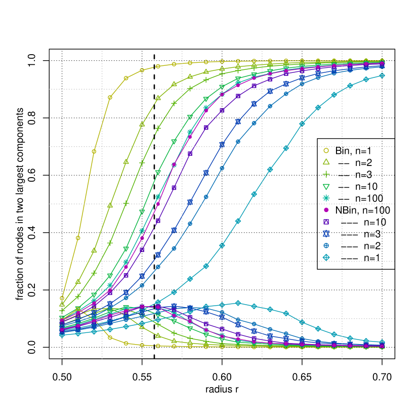
Fig. 4: Mean fractions of nodes in the two largest components of the sub- and super-Poisson Boolean models $C(\Phi^{pert}_{{\rm Binom}(n,1/n)},r)$ and $C(\Phi^{pert}_{\mathrm{NBionom}(n,1/(1+n))},r)$ , respectively, as functions of $r$. These families of underlying point processes converge to the Poisson point process $\Phi_{\lambda}$ with intensity $\lambda=2/(\sqrt{3})=1.154701$ as $n$ tends to $\infty$; cf. Example 18. The dashed vertical line corresponds to the radius $r=0.5576495$ which is believed to be close to the critical radius $r_{c}(\Phi_{\lambda})$.

But it turns out that the conjecture is not true in full generality and a counterexample was also presented in dcx-perc . It is a Poisson-Poisson cluster point process, which is known to be super-Poisson (cf. Example 16) whose critical radius is $r_{c}=0$, hence smaller than that of the corresponding Poisson point process, for which $r_{c}$ is known to be positive. In this Poisson-Poisson cluster point process, points concentrate on some carefully chosen larger-scale structure, which itself has good percolation properties. In this case, the points concentrate in clusters, however we cannot say that clusters are well spaced out. Hence, this example does not contradict our initial heuristic explanation of why an increase of clustering in a point process should increase the critical radius for the percolation. It reveals rather that dcx-ordering, while being able to compare the clustering tendency of point processes, is not capable of comparing macroscopic structures of clusters. Nevertheless, dcx-ordering, and some weaker tools introduced in Sect. 3, can be used to prove nontrivial phase transitions for point processes which cluster less than the Poisson process. In what follows, we will first present some intuitions leading to the above results and motivating our special focus on moment measures and void probabilities in the previous sections.

Intuitions — Some Non-Standard Critical Radii

Consider the radii $\underline{r}_{c},\overline{r}_{c}$, which act as lower and upper bounds for the usual critical radius: i.e. $\underline{r}_{c}\leq r_{c}\leq\overline{r}_{c}$. We show that clustering acts differently on these bounding radii: It turns out that

$$\underline{r}_{c}(\Phi_{2})\leq\underline{r}_{c}(\Phi_{1})\leq r_{c}(\Phi_{1})\leq\overline{r}_{c}(\Phi_{1})\leq\overline{r}_{c}(\Phi_{2})$$

for $\Phi_{1}$ having smaller voids and moment measures than $\Phi_{2}$. This sandwich inequality tells us that $\Phi_{1}$ exhibits the usual phase transition $0<r_{c}(\Phi_{1})<\infty$, provided $\Phi_{2}$ satisfies the stronger conditions $0<\underline{r}_{c}(\Phi_{2})$ and $\overline{r}_{c}(\Phi_{2})<\infty$. Conjecturing that this holds if $\Phi_{2}$ is a Poisson point process, one obtains the result on (uniformly) non-trivial phase transition for all weakly sub-Poisson processes $\Phi_{1}$, which has been proved in dcx-perc and will be presented in the subsequent sections in a slightly different way.

Let $\Phi$ be an arbitrary point process in $\mathbb{R}^{d}$. Let $W_{m}=[-m,m]^{d}$ and define $h_{m,k}:(\mathbb{R}^{d})^{k}\to\{0,1\}$ to be the indicator of the event that ${x_{1},\ldots,x_{k}}\in(\Phi\cap W_{m})^{k},|x_{1}|\leq r,\inf_{x\in\partial W_{m}}|x-x_{k}|\leq r,\max_{i\in\{1,\ldots,k-1\}}|x_{i+1}-x_{i}|\leq r$, where $\partial W_{n}$ denotes the boundary of set $W_{n}$. Let $N_{m,k}(\Phi,r)=\sum^{\neq}_{X_{1},\allowbreak\ldots,X_{k}\in\mathbb{R}^{d}}h_{m,k}(X_{1},\ldots,X_{k})$ denote the number of distinct self-avoiding paths of length $k$ from the origin $o\in\mathbb{R}^{2}$ to the boundary of the box $W_{m}$ in the Boolean model and $N_{m}(\Phi,r)=\sum_{k\geq 1}N_{m,k}(\Phi,r)$ to be the total number of distinct self-avoiding paths to the boundary of the box. We define the following “lower” critical radius

$${\underline{r}}_{c}(\Phi)=\inf\{r:\liminf_{m}\mathbf{E}N_{m}(\Phi,r)>0\}\,.$$

Note that $r_{c}(\Phi)=\inf\{r:\lim_{m\to\infty}\mathbf{P}\left(N_{m}(\Phi,r)\geq 1\right)>0\}$, with the limit existing because the events $\{N_{m}(\Phi,r)\geq 1\}$ form a decreasing sequence in $m$, and by Markov’s inequality, we have that indeed ${\underline{r}}_{c}(\Phi)\leq r_{c}(\Phi)$ for a stationary point process $\Phi$.

It is easy to see that $\mathbf{E}N_{m}(\Phi,r)$ can be expressed in terms of moment measures, i.e. $\mathbf{E}N_{m}(\Phi,r)=\sum_{k\geq 1}\mathbf{E}N_{m,k}(\Phi,r)$ and

$$\mathbf{E}N_{m,k}(\Phi,r)=\int_{(\mathbb{R}^{d})^{k}}h_{m,k}(x_{1},\ldots,x_{k})\alpha_{j}^{(k)}(\mathrm{d}x_{1},\ldots,\mathrm{d}x_{k}).$$

The following result is obtained in dcx-clust .

Proposition 13

Let $C_{j}=C(\Phi_{j},r)$, $j=1,2$ be two Boolean models with simple point processes of germs $\Phi_{j}$, $j=1,2,$ and $\sigma$-finite $k$-th moment measures $\alpha_{j}^{k}$ for all $k\geq 1$ respectively. If $\alpha_{1}^{(k)}(\cdot)\leq\alpha_{2}^{(k)}(\cdot)$ for all $k\geq 1$, then ${\underline{r}}_{c}(\Phi_{1})\geq{\underline{r}}_{c}(\Phi_{2}).$ In particular, for a stationary, $\alpha$-weakly sub-Poisson point process $\Phi_{1}$ with unit intensity, it holds that $\kappa_{d}{\underline{r}}_{c}(\Phi_{1})^{d}\geq 1$ where $\kappa_{d}$ is the volume of the unit ball in $\mathbb{R}^{d}$.

In order to see void probabilities in action it is customary to use some discrete approximations of the continuum percolation model. For $r>0,x\in\mathbb{R}^{d}$, define the following subsets of $\mathbb{R}^{d}$. Let $Q^{r}=(-\frac{1}{2r},\frac{1}{2r}]^{d}$ and $Q^{r}(x)=x+Q^{r}.$ We consider the following discrete graph parametrised by $n\in\mathbb{N}$. Let $\mathbb{L}^{*d}_{n}=(\mathbb{Z}^{d}_{n},\mathbb{E}^{*d}_{n})$ be the usual close-packed lattice graph scaled down by the factor $1/n$. It holds that $\mathbb{Z}^{d}_{n}=\frac{1}{n}\mathbb{Z}^{d}$ for the set of vertices and $\mathbb{E}^{*d}_{n}=\{\langle z_{i},z_{j}\rangle\in(\mathbb{Z}^{d}_{n})^{2}:Q^{\frac{n}{2}}(z_{i})\cap Q^{\frac{n}{2}}(z_{j})\neq\emptyset\}$ for the set of edges, where $\mathbb{Z}$ denotes the set of integers.

A contour in $\mathbb{L}^{*d}_{n}$ is a minimal collection of vertices such that any infinite path in $\mathbb{L}^{*d}_{n}$ from the origin has to contain one of these vertices (the minimality condition implies that the removal of any vertex from the collection will lead to the existence of an infinite path from the origin without any intersection with the remaining vertices in the collection). Let $\Gamma_{n}$ be the set of all contours around the origin in $\mathbb{L}^{*d}_{n}$. For any subset of points $\gamma\subset\mathbb{R}^{d}$, in particular for paths $\gamma\in\Gamma_{n}$, we define $Q_{\gamma}=\bigcup_{z\in\gamma}Q^{n}(z)$.

With this notation, we can define the “upper” critical radius ${\overline{r}}_{c}(\Phi)$ by

$${\overline{r}}_{c}(\Phi)=\inf\Bigl{\{}r>0:\text{for all}\;n\geq 1,\sum_{\gamma\in\Gamma_{n}}\mathbf{P}\left(C(\Phi,r)\cap Q_{\gamma}=\emptyset\right)<\infty\Bigr{\}}\,.$$ (14)

It might be seen as the critical radius corresponding to the phase transition when the discrete model $\mathbb{L}^{*d}_{n}=(\mathbb{Z}^{d}_{n},\mathbb{E}^{*d}_{n})$, approximating $C(\Phi,r)$ with an arbitrary precision, starts percolating through the Peierls argument. As a consequence, ${\overline{r}}_{c}(\Phi)\geq r_{c}(\Phi)$ (see (perc-dcx, , Lemma 4.1)). The following ordering result follows immediately from the definitions.

Corollary 1

Let $C_{j}=C(\Phi_{j},r)$, $j=1,2$ be two Boolean models with simple point processes of germs $\Phi_{j}$, $j=1,2$. If $\Phi_{1}$ has smaller voids probabilities then $\Phi_{2}$, then ${\overline{r}}_{c}(\Phi_{1})\leq{\overline{r}}_{c}(\Phi_{2})$.

Remark 6

The finiteness of ${\overline{r}}_{c}$ is not clear even for Poisson point process and hence Corollary 1 cannot be directly used to prove the finiteness of the critical radii of $v$-weakly sub-Poisson point processes. However, the approach based on void probabilities can be refined, as we shall see in what follows, to conclude the aforementioned property.

Percolation of Level-Sets of Shot-Noise Fields

Various percolation problems, including the classical continuum percolation model considered in the previous section, can be posed as percolation of some level sets of shot-noise fields. We say that a level set percolates if it has an unbounded connected subset. We now present a useful lemma that can be used in conjunction with other methods, in particular the famous Peierls argument (cf. (Grimmett99, , pp. 17–18)), to exhibit percolation of the level sets of shot-noise fields for an appropriate choice of parameters. We sketch these arguments in the simple case of the Boolean model and the application to the SINR model in the subsequent sections. The proofs rely on coupling of a discrete model with the continuum model and showing percolation or non-percolation in the discrete model using the above bounds.

In what follows we will be interested in level-sets of shot-noise fields, i.e. sets of the form $\{y\in S:V_{\Phi}(y)\geq{a}\}$ or $\{y\in S:V_{\Phi}(y)\leq{a}\}$ for some ${a}\in\mathbb{R}$, where $\{V_{\Phi}(y),y\in S\}$ is a shot-noise field generated by some point process $\Phi$ with a non-negative response function $h$ as introduced in Definition 14. For proving results on percolation of level-sets, we rely heavily on the bounds from the following lemma.

Lemma 1 ((dcx-perc, , Lemma 3.2))

Let $\Phi$ be a stationary point process with positive and finite intensity $\lambda$. Then the following statements are true.

1. If $\Phi$ is $\alpha$-weakly sub-Poisson, then

   $$\mathbf{P}\left(\min_{i\in\{1,\ldots,m\}}V_{\Phi}(y_{i})\geq{a}\right)\leq e^{-sm{a}}\exp\lambda\int_{\mathbb{R}^{d}}(e^{s\sum_{i=1}^{m}{h}(x,y_{i})}-1)\mathrm{d}x$$ (15)

   for any $y_{1},\ldots,y_{m}\in S$ and $s>0$.

2. If $\Phi$ is $v$-weakly sub-Poisson then,

   $$\mathbf{P}\left(\max_{i\in\{1,\ldots,m\}}V_{\Phi}(y_{i})\leq{a}\right)\leq e^{-sm{a}}\exp\left(\lambda\int_{\mathbb{R}^{d}}(e^{s\sum_{i=1}^{m}{h}(x,y_{i})}-1)\mathrm{d}x\right)$$ (16)

   for any $y_{1},\ldots,y_{m}\in S$ and $s>0$.

Proof

Observe that $\sum_{i=1}^{m}V_{\Phi}(y_{i})=\sum_{X\in\Phi}\sum_{i=1}^{m}{h}(X,y_{i})$ is itself a shot-noise field driven by the response function $\sum_{i=1}^{m}{h}(.,y_{i}).$ Thus if (15) and (16) are true for $m=1$, we can derive the general case as well. Using Chernoff’s bound, we have that $\mathbf{P}\left(V_{\Phi}(y)\geq{a}\right)\leq e^{-s{a}}\mathbf{E}\left(e^{sV_{\Phi}(y)}\right)$ and $\mathbf{P}\left(V_{\Phi}(y)\leq{a}\right)\leq e^{s{a}}\mathbf{E}\left(e^{-sV_{\Phi}(y)}\right)$. The two statements now follow from Propositions 2 and  3 respectively.     

$k$-Percolation in the Boolean Model

By $k$-percolation in a Boolean model, we understand percolation of the subset of the space covered by at least $k$ grains of the Boolean model; cf. Definition 15. Our aim is to show that for sub-Poisson point processes (i.e. point processes that are dcx-smaller than the Poisson point process) or negatively associated point processes, the critical connection radius $r$ for $k$-percolation of the Boolean model is non-degenerate, i.e., the model does not percolate for $r$ too small and percolates for $r$ sufficiently large. As will be seen in the proof given below, the finiteness of the critical radius $r$ for $k=1$ (i.e. the usual percolation) holds under a weaker assumption of ordering of void probabilities.

Given a point processes of germs $\Phi$ on $\mathbb{R}^{d}$, we define the coverage field $\{V_{\Phi,r}(x),\allowbreak x\in\mathbb{R}^{d}\}$ by $V_{\Phi,r}(x)=\sum_{X\in\Phi}\mathbf{1}(x\in B_{r}(X))$, where $B_{r}(x)$ denotes the Euclidean ball of radius $r$ centred at $x$. The $k$-covered set is defined as the following level set. Let $C_{k}(\Phi,r)=\{x\in\mathbb{R}^{d}:V_{\Phi,r}(x)\geq k\}$. Note that $C_{1}(\Phi,r)=C(\Phi,r)$ is the usual Boolean model. For $k\geq 1$, define the critical radius for $k$-percolation as

$$r^{k}_{c}(\Phi)=\inf\{r:\mathbf{P}(\mbox{$C_{k}(\Phi,r)$ percolates})>0\}\,,$$

where, as before, percolation means existence of an unbounded connected subset. Clearly, $r_{c}^{1}(\Phi)=r_{c}(\Phi)\leq r_{c}^{k}(\Phi)$. As in various percolation models, the first question is whether $0<r^{k}_{c}(\Phi)<\infty$ ? This is known for the Poisson point process (Gilbert61 ) and not for many other point processes apart from that. The following result is a first step in that direction answering the question in affirmative for many point processes.

Proposition 14 ( (dcx-perc, , Proposition. 3.4))

Let $\Phi$ be a stationary point processes with intensity $\lambda$. For $k\geq 1,\lambda>0$, there exist constants $c(\lambda)$ and $C(\lambda,k)$ (not depending on the distribution of $\Phi$) such that $0<c(\lambda)\leq r_{c}^{1}(\Phi)$ provided $\Phi$ is $\alpha$-weakly sub-Poisson and $r_{c}^{k}(\Phi)\leq C(\lambda,k)<\infty$ provided $\Phi$ is $v$-weakly sub-Poisson. Consequently, for $\Phi$ being weakly sub-Poisson, combining both the above statements, it turns out that

$$0<c(\lambda)\leq r_{c}^{1}(\Phi)\leq r_{c}^{k}(\Phi)\leq C(\lambda,k)<\infty.$$

Remark 7

The above result not only shows non-triviality of the critical radius for stationary weakly sub-Poisson processes but also provides uniform bounds. Examples of particular point processes for which this non-triviality result holds are determinantal point processes with trace-class integral kernels (cf. Definition 6 and Example 12) and Voronoi-perturbed latices with convexly sub-Poisson replication kernels (cf. Example 3). For the case of zeros of Gaussian analytic functions which is not covered by us, a non-trivial critical radius for continuum percolation has been shown in Ghosh12 , where uniqueness of infinite clusters for both zeros of Gaussian analytic functions and the Ginibre point process is also proved.

Sketch of Proof (of Proposition 14)

A little more notation is required. For $r>0,x\in\mathbb{R}^{d}$, define the following subsets of $\mathbb{R}^{d}$. Let $Q_{r}=(-r,r]^{d}$ and $Q_{r}(x)=x+Q_{r}$. Furthermore, we consider the following discrete graph. Let $\mathbb{T}^{*d}(r)=(r\mathbb{Z}^{d},\mathbb{E}^{*d}(r))$ be a close-packed graph on the scaled-up lattice $r\mathbb{Z}^{d}$; the edge-set is given by $\mathbb{E}^{*d}(r)=\{\langle z_{i},z_{j}\rangle\in(r\mathbb{Z}^{d})^{2}:Q_{r}(z_{i})\cap Q_{r}(z_{j})\neq\emptyset\}$. Recall that by site-percolation in a graph one means the existence of an infinite connected component in the random subgraph that remains after deletion of sites/vertices as per some random procedure. In order to prove the first statement, let $\Phi$ be $\alpha$-weakly sub-Poisson and $r>0$. Consider the close-packed lattice $\mathbb{T}^{*d}({3}r)$. Define the response function ${h_{r}}(x,y)=\mathbf{1}(x\in Q_{{3r/2}}(y))$ and the corresponding shot-noise field $V^{r}_{\Phi}(.)$ on $\mathbb{T}^{*d}({3}r)$. Note that if $C(\Phi,r)$ percolates then $\{z:V^{r}_{\Phi}(z)\geq 1\}$ percolates on $\mathbb{T}^{*d}({3}r)$ as well. We shall now show that there exists a $r>0$ such that the latter does not hold true. To prove this, we show that the expected number of paths from $o$ of length $n$ in the random subgraph tends to $0$ as $n\to\infty$ and Markov’s inequality gives that there is no infinite path (i.e. no percolation) in $\mathbb{T}^{*d}({3}r)\cap\{z:V^{r}_{\Phi}(z)\geq 1\}.$ There are $(3^{d}-1)^{n}$ paths of length $n$ from $o$ in $\mathbb{T}^{*d}(2r)$ and the probability that a path $z_{i}\in r\mathbb{Z}^{d},1\leq i\leq n$ is open can be bounded from above as follows. Using (15) and some further calculations, we get that

$$\mathbf{P}\left(\min_{i\in\{1,\ldots,n\}}V^{r}_{\Phi}(z_{i})\geq 1\right)\leq(\exp\{-(s+(1-e^{s})\lambda(3r)^{d})\})^{n}.$$

So, the expected number of paths from $o$ of length $n$ in $\mathbb{T}^{*d}(3r)\cap\{z:V^{r}_{\Phi}(z)\geq 1\}$ is at most $((3^{d}-1)\exp\{-(s+(1-e^{s})\lambda(3r)^{d})\})^{n}$. This term tends to $0$ as $n\to\infty$ for $r$ small enough and $s$ large enough. Since the choice of $r$ depends only on $\lambda$, we have shown that there exists a constant $c(\lambda)>0$ such that $c(\lambda)\leq r_{c}^{1}(\Phi).$ For the upper bound, let $\Phi$ be $\nu$-weakly sub-Poisson and consider the close-packed lattice $\mathbb{T}^{*d}(\frac{r}{\sqrt{d}})$. Define the response function ${h_{r}}(x,y)=\mathbf{1}(x\in Q_{{\frac{r}{\sqrt{d}}}}(y))$ and the corresponding additive shot-noise field $V^{r}_{\Phi}(\cdot).$ Note that if the random subgraph $\mathbb{T}^{*d}(\frac{r}{\sqrt{d}})\cap\{z:V^{r}_{\Phi}(z)\geq{k}\}$ percolates, then $C(\Phi,r)$ also percolates. Then, the following exponential bound is obtained by using (16) and some more calculations:

$$\mathbf{P}(\max_{i\in\{1,\ldots,n\}}V^{r}_{\Phi}(z_{i})\leq{k}-1)\leq{(}\exp\{-((1-e^{-s})\lambda(\frac{r}{\sqrt{d}})^{d}-s({k}-1))\})^{n}.\,\,\,\,\,$$

It now suffices to use the standard Peierls argument (cf. (Grimmett99, , pp. 17–18)) to complete the proof.     

For $k=1$; i.e., for the usual percolation in the Boolean model, we can avoid the usage of the exponential estimates of Lemma 1 and work directly with void probabilities and factorial moment measures. This leads to improved bounds on the critical radius.

Proposition 15 ( (dcx-perc, , Corollary 3.11))

For a stationary weakly sub-Poisson point process $\Phi$ on $\mathbb{R}^{d}$, $d\geq 2$, it holds that

$$0<\frac{1}{(\lambda\kappa_{d})^{1/d}}\leq r_{c}(\Phi)\leq\sqrt{d}\left(\frac{\log(3^{d}-2)}{\lambda}\right)^{1/d}<\infty,$$

where $\kappa_{d}$ is the volume of the unit ball in $\mathbb{R}^{d}$. The lower and the upper bounds hold, respectively, for $\alpha$-weakly $\nu$-weakly sub-Poisson processes.

Remark 8

Applying the above result to an $\alpha$-weakly sub-Poisson point processes with unit intensity we observe that $r_{c}(\Phi)\geq\kappa_{d}^{-\frac{1}{d}}\to\infty$ as $d\to\infty.$ This means that in high dimensions, it holds that $r_{c}(\Phi)\gg r_{c}(\mathbb{Z}^{d})=\frac{1}{2}$, i.e. like the Poisson point process and even sub-Poisson point processes percolate much worse compared to the Euclidean lattice in high dimensions.

However, the question remains open whether the initial heuristic reasoning saying that more clustering worsens percolation (cf. p. 4.1) holds for sub-Poisson point processes. As we have seen and shall see below, sub-Poisson point processes are more tractable than super-Poisson point processes in many respects.

SINR Percolation

For a detailed background about this model of wireless communications, we refer to subpoisson and the references therein. Here we directly begin with a formal introduction to the model. We shall work only in $\mathbb{R}^{2}$ in this section.

The parameters of the model are the non-negative numbers $P$ (signal power), $N$ (environmental noise), $\gamma$, $T$(SINR threshold) and an attenuation function $\ell:\mathbb{R}^{2}_{+}\to\mathbb{R}_{+}$ satisfying the following assumptions: $\ell(x,y)=l(|x-y|)$ for some continuous function $l:\mathbb{R}_{+}\to\mathbb{R}_{+}$, strictly decreasing on its support, with $l(0)\geq TN/P$, $l(\cdot)\leq 1$, and $\int_{0}^{\infty}xl(x)\mathrm{d}x<\infty$. These are exactly the assumptions made in Dousse_etal06 and we refer to this article for a discussion on their validity.

Given a point processes $\Phi$, the interference generated due to the point processes at a location $x$ is defined as the following shot-noise field $\{I_{\Phi}(x),x\in\mathbb{R}^{d}\}$, where $I_{\Phi}(x)=\sum_{X\in\Phi\setminus\{x\}}l(|X-x|)$. Define the signal-to-noise ratio (SINR) as follows :

$$\text{SINR}(x,y,\Phi,\gamma)=\frac{Pl(|x-y|)}{N+\gamma PI_{\Phi\setminus\{x\}}(y)}.$$ (17)

Let $\Phi_{B}$ and $\Phi_{I}$ be two point processes. Furthermore, let $P,N,T>0$ and $\gamma\geq 0$. The SINR graph is defined as $\mathbb{T}(\Phi_{B},\Phi_{I},\gamma)=(\Phi_{B},\mathbb{E}(\Phi_{B},\Phi_{I},\gamma))$ where

$$\mathbb{E}(\Phi_{B},\Phi_{I},\gamma)=\{\langle X,Y\rangle\leavevmode\nobreak\ \in\leavevmode\nobreak\ \Phi_{B}^{2}:\min\{SINR(Y,X,\Phi_{I},\gamma),SINR(X,Y,\Phi_{I},\gamma)\}>T\}.$$

The SNR graph (i.e. the graph without interference, $\gamma=0$) is defined as $\mathbb{T}(\Phi_{B})=\mathbb{T}(\Phi_{B},\emptyset,0)$ and this is nothing but the Boolean model $C(\Phi_{B},r_{l})$ with $2r_{l}=l^{-1}(\frac{TN}{P})$.

Recall that percolation in the above graphs is the existence of an infinite connected component in the graph-theoretic sense. Denote by $\lambda_{c}(r)=\lambda(r_{c}(\Phi_{\lambda})/r)^{2}$ the critical intensity for percolation of the Boolean model $C(\Pi_{\lambda},r)$. There is much more dependency in this graph than in the Boolean model where the edges depend only on the two corresponding vertices, but still we are able to suitably modify our techniques to obtain interesting results about non-trivial phase-transition in this model. More precisely, we are showing non-trivial percolation in SINR models with weakly sub-Poissonian set of transmitters and interferers and thereby considerably extending the results of Dousse_etal06 . In particular, the set of transmitters and interferers could be stationary determinantal point processes or sub-Poisson perturbed lattices and the following result still guarantees non-trivial phase transition in the model.

Proposition 16 ( (dcx-perc, , Propositions 3.9 and 3.10))

The following statements are true.

1. Let $\lambda>\lambda_{c}(r_{l})$ and let $\Phi$ be a stationary $\alpha$-weakly sub-Poisson point process with intensity $\mu$ for some $\mu>0$. Then there exists $\gamma>0$ such that $\mathbb{T}(\Pi_{\lambda},\Phi,\gamma)$ percolates.

2. Let $\Phi$ be a stationary, $\gamma$-weakly sub-Poisson point processes and let $\Phi_{I}$ be a stationary $\alpha$-weakly sub-Poisson point process with intensity $\mu$ for some $\mu>0.$ Furthermore, assume that $l(x)>0$ for all $x\in\mathbb{R}_{+}$. Then there exist $P,\gamma>0$ such that $\mathbb{T}(\Phi,\Phi_{I},\gamma)$ percolates.

Exercise 13

Two related percolation models are the $k$-nearest neighbourhood graph ($k$-NNG) and the random connection model. Non-trivial phase transitions for percolation is shown for both models when defined on a Poisson point process in (Franc_etal07, , Sect. 2.4 and 2.5). We invite the reader to answer the challenging question of whether the methods of Franc_etal07 combined with ours could be used to show non-trivial phase transition for weakly sub-Poisson point processes, too. Hint. The results of Daley05 on the Lilypond model could be useful to show non-percolation for $1$-NNG.

4.2 U-Statistics of Point Processes

Denote by $\Phi^{(k)}(\mathrm{d}(x_{1},\ldots,x_{k}))=\Phi(\mathrm{d}x_{1})\left(\Phi\setminus\delta_{x_{1}}\right)(\mathrm{d}x_{2})\dots\left(\Phi\setminus\sum_{i=1}^{k-1}\delta_{x_{i}}\right)(\mathrm{d}x_{k})$ the (empirical) $k$-th order factorial moment measure of $\Phi$. Note that this is a point process on $\mathbb{R}^{dk}$ with mean measure $\alpha^{(k)}$. In case when $\Phi$ is simple, $\Phi^{(k)}$ is simple too and corresponds to the point process of ordered $k$-tuples of distinct points of $\Phi$.

In analogy with classical U-statistics, a U-statistic of a point process $\Phi$ can be defined as the functional $F(\Phi)=\sum_{X\in\Phi^{(k)}}f(X)$, for a non-negative symmetric function $f$ (Reitzner11 ). In case when $\Phi$ is infinite one often considers $F(\Phi\cap W)$, where $W\subset\mathbb{R}$ is a bounded Borel set. The reader is referred to Reitzner11 or (Schulte12, , Sect. 2) for many interesting U-statistics of point processes of which two — subgraphs in a random geometric graph ((Penrose03, , Chap. 3)) and simplices in a random geometric complex (see (Yukich12, , Sect. 8.4.4)) — are described below.

Examples

Example 20 (Subgraphs counts in a random geometric graph)

Let $\Phi$ be a finite point process and $r>0.$ The random geometric graph $\mathbb{T}(\Phi,r)=(\Phi,\mathbb{E}(\Phi,r))$ is defined through its vertices and edges, where the edge set is given by $\mathbb{E}(\Phi,r)=\{(X,Y)\in\Phi:|X-Y|\leq r\}$. For a connected subgraph $\Gamma$ on $k$ vertices, define $h:\mathbb{R}^{dk}\to\{0,1\}$ by $h_{\Gamma,r}(x)=\mathbf{1}(\mathbb{T}(x,r)\cong\Gamma)$, where $\cong$ stands for graph isomorphism. Now, the number of $\Gamma$-induced subgraphs in $\Phi$ is defined as

$$G_{r}(\Phi,\Gamma)=\frac{1}{k!}\sum_{X\in\Phi^{(k)}}h_{\Gamma,r}(X).$$

Clearly, $G_{r}(\Phi,\Gamma)$ is a U-statistic of $\Phi.$ In the special case that $|\Gamma|=2$, then $G_{r}(\Phi,\Gamma)$ is the number of edges.

Example 21 (Simplices counts in a random geometric simplex)

A non-empty family of finite subsets $\Delta(S)$ of a set $S$ is an abstract simplicial complex if for every set $X\in\Delta(S)$ and every subset $Y\subset X$, we have that $Y\in\Delta(S)$. We shall from now on drop the adjective “abstract”. The elements of $\Delta(S)$ are called faces resp. simplices of the simplicial complex and the dimension of a face $X$ is $|X|-1$. Given a finite point process $\Phi$, one can define the following two simplicial complexes : The Čech complex $Ce(\Phi,r)$ is defined as the simplicial complex whose $k$-faces are $\{X_{0},\ldots,X_{k}\}\subset\Phi$ such that $\cap_{i}B_{r}(X_{i})\neq\emptyset.$ The Vietoris-Rips complex $VR(\Phi,r)$ is defined as the simplicial complex whose $k$-faces are $\{X_{0},\ldots,X_{k}\}\subset\Phi$ such that $B_{r}(X_{i})\cap B_{r}(X_{j})\neq\emptyset$ for all $0\leq i\neq j\leq k.$ The $1$-skeleton (i.e. the subcomplex consisting of all $0$-faces and $1$-faces) of the two complexes are the same and it is nothing but the random geometric graph $\mathbb{T}(\Phi,r)$ of Example 20. Also, the Čech complex $Ce(\Phi,r)$ is homotopy equivalent to the Boolean model $C(\Phi,r)$. The number of $k$-faces in the two simplicial complexes can be determined as follows:

$$S_{k}(Ce(\Phi,r)) = \frac{1}{k!}\sum_{X\in\Phi^{(k)}}\mathbf{1}(X\mbox{ is a $k$-face of $Ce(\Phi,r)$})$$

and similarly for $S_{k}(VR(\Phi,r))$. Clearly, both characteristics are examples of U-statistics of $\Phi$.

Note that a U-statistic is an additive shot-noise of the point process $\Phi^{(k)}$ and this suggests the applicability of our theory to U-statistics. Speaking a bit more generally, consider of a family of U-statistics $\mathsf{K}$ and define an additive shot-noise field $\{F(\Phi)\}_{F\in\mathsf{K}}$ indexed by $\mathsf{K}$. Why do we consider such an abstraction? Here is an obvious example.

Example 22

Consider $\mathsf{K}=\{F_{B},F_{B}(\Phi)=\sum_{X\in\Phi^{(k)}}\mathbf{1}(f(X)\in B)\}_{B\in B_{0}(\mathbb{R}_{+})}$ for some given non-negative symmetric function $f$ defined on $\mathbb{R}^{k}$. Then the additive shot-noise field on $\Phi^{(k)}$, indexed by bounded Borel sets $B\in\mathbb{R}_{+}$, defined above is nothing but the random field characterising the following point process on $\mathbb{R}_{+}$ associated to the U-statistics of $\Phi$:

$$\eta_{(f,\Phi)}=\{f(X):X\in\Phi^{(k)}\}\,$$

in the sense that $F_{B}(\Phi)=\eta_{(f,\Phi)}(B)$. (Note that if $|f^{-1}([0,x])|<\infty$ for all $x\in\mathbb{R}_{+}$, then $\eta_{\Phi}$ is indeed locally finite and hence a point process and we always assume that $f$ satisfies such a condition.) This point process has been studied in Schulte12 , in the special case when $\Phi=\Pi_{\lambda}$ is a homogeneous Poisson point process. It is shown that if $\lambda\to\infty$, then $\eta_{(f,\Phi)}$ tends to a Poisson point process with explicitly known intensity measure.

For any U-statistic $F$ and for a bounded window $W\subset\mathbb{R}^{d}$, we have that

$$\mathbf{E}F(\Phi\cap W)=\frac{1}{k!}\int_{W}f(x_{1},\ldots,x_{k})\alpha^{(k)}\mathrm{d}(x_{1},\ldots,x_{k}).$$

Similarly, we can express higher moments of the shot-noise field $\{F(\Phi)\}_{F\in\mathsf{K}}$ by those of $\Phi$. With these observations in hand and using Proposition 9, we can state the following result.

Proposition 17

Let $\Phi_{1},\Phi_{2}$ be two point processes with respective factorial moment measures $\alpha_{i}^{(k)}$, $i=1,2$ and let $W$ be a bounded Borel set in $\mathbb{R}^{d}$. Consider a family $\mathsf{K}$ of U-statistics. Then the following statements are true.

1. If $\alpha_{1}^{(j)}(\cdot)\leq\alpha_{2}^{(j)}(\cdot)$ for all $1\leq j\leq k$, then

   $$\mathbf{E}(F_{1}(\Phi_{1}\cap W)F_{2}(\Phi_{1}\cap W)\ldots F_{k}(\Phi_{1}\cap W))\leq\mathbf{E}(F_{1}(\Phi_{2}\cap W)F_{2}(\Phi_{2}\cap W)\ldots F_{k}(\Phi_{2}\cap W))$$

   for any $k$-tuple of U-statistics $F_{1},\ldots,F_{k}\in\mathsf{K}$. In particular, for any given $F\in\mathsf{K}$ based on a non-negative symmetric function $f$ it holds that $\alpha_{\eta_{(f,\Phi_{1})}}^{(k)}(\cdot)\leq\alpha_{\eta_{(f,\Phi_{2})}}^{(k)}(\cdot)$, where $\alpha_{\eta_{(f,\Phi_{i})}}^{(k)}$ is the $k$-th order factorial moment measure of $\eta_{(f,\Phi_{i})}$.

2. If $\Phi_{1}\leq_{\rm{dcx}}\Phi_{2}$, then $\{F(\Phi_{1}\cap W)\}_{F\in\mathsf{K}}\leq_{\rm{idcx}}\{F(\Phi_{2}\cap W)\}_{F\in\mathsf{K}}$ and in particular $\eta_{(f,\Phi_{1})}\leq_{\rm{idcx}}\eta_{(f,\Phi_{2})}$.

Some Properties of Random Geometric Graphs

The subgraph count $G_{r}(\cdot,\cdot)$ considered in Example 20 is only a particular example of a U-statistic but its detailed study in the case of the Poisson point process (see (Penrose03, , Chap. 3)) was the motivation to derive results about subgraph counts of a random geometric graph over other point processes (Adler12 ). Here, we explain some simple results about clique numbers, maximal degree and chromatic number that can be deduced as easy corollaries of ordering of subgraph counts known due to Proposition 17.

Slightly differing from Penrose03 , we consider the following asymptotic regime for a stationary point process $\Phi$ with unit intensity. We look at the properties of $\mathbb{T}(\Phi_{n},r_{n})$, $n\geq 1$, where $\Phi_{n}=\Phi\cap W_{n}$ with $W_{n}=[-\frac{n^{\frac{1}{d}}}{2},\frac{n^{\frac{1}{d}}}{2}]^{d}$ and a radius regime $r_{n}.$ To compare our results with those of Penrose03 , replace the $r_{n}^{d}$ factor in our results by $nr_{n}^{d}.$ Detailed asymptotics of $G_{n}(\Phi_{n},\Gamma)=G_{r_{n}}(\Phi_{n},\Gamma)$ for general stationary point processes have been studied in (Adler12, , Sect. 3).

Let $\mathcal{C}_{n}=\mathcal{C}_{n}(\Phi),\Delta_{n}=\Delta_{n}(\Phi),\mathcal{X}_{n}=\mathcal{X}_{n}(\Phi)$ denote the size of the largest clique, maximal vertex degree and chromatic number of $\mathbb{T}(\Phi_{n},r_{n})$, respectively. Heuristic arguments for these quantities say that they should increase with more clustering in the point process. We give a more formal statement of this heuristic at the end of this section.

Let $\Gamma_{k}$ denote the complete graph on $k$ vertices and $\Gamma^{{}^{\prime}}_{1},\ldots,\Gamma^{{}^{\prime}}_{m}$ be the maximum collection of non-isomorphic graphs on $k$ vertices having maximum degree $k-1.$ Then for $k\geq 1$, we have the following two equalities and the graph-theoretic inequality that drive the result following them: $\{\mathcal{C}_{n}<k\}=\{G_{n}(\Phi_{n},\Gamma_{k})=0\}$, $\{\Delta_{n}<k-1\}=\cap_{i=1}^{m}\{G_{n}(\Phi_{n},\Gamma^{{}^{\prime}}_{i})=0\}$, $\mathcal{C}_{n}\leq\mathcal{X}_{n}\leq\Delta_{n}+1$.

Corollary 2

Let $\Phi$ be a stationary $\alpha$-weakly sub-Poisson point process with unit intensity. If $nr_{n}^{d(k-1)}\to 0$, then

$$\lim_{n\to\infty}\mathbf{P}(\mathcal{C}_{n}<k)=\lim_{n\to\infty}\mathbf{P}(\Delta_{n}<k-1)=\lim_{n\to\infty}\mathbf{P}(\mathcal{X}_{n}<k)=1.$$

Sketch of Proof

To prove the result for $\mathcal{C}_{n}$, due to Markov’s inequality and the fact that $\mathbf{E}G_{n}(\Phi_{n},\Gamma)\leq\mathbf{E}G_{n}(\Pi_{1_{n}},\Gamma)$ (see Proposition 17), it suffices to show that $\mathbf{E}G_{n}(\Pi_{1_{n}},\Gamma)\to 0$ for $nr_{n}^{d(k-1)}\to 0$ and any graph $\Gamma$ on $k$ vertices. This is already known from (Penrose03, , Theorem 6.1). The proof for $\Delta_{n}$ is similar and it also proves the result for $\mathcal{X}_{n}$.     

Note that if $k=2$, the results of Corollary 2 implies that $\lim_{n\to\infty}\mathbf{P}(\mathcal{C}_{n}=1)=1$ by using the trivial lower bound of $\mathcal{C}_{n}\geq 1$, and analogously for the other two quantities. To derive a similar result for $k\geq 2,$ we need variance bounds for $G_{n}(\cdot,\cdot)$ to use the standard second moment method. These variance bounds for $G_{n}(\cdot,\cdot)$ are available in the case of negatively associated point processes (see (Adler12, , Sect. 3.4)).

Further, for point processes with $\alpha^{(k)}$ admitting a continuous density $\alpha^{(k)}(\mathrm{d}(x_{1},\ldots,\allowbreak x_{k}))=\rho^{(k)}(x_{1},\ldots,x_{k})\mathrm{d}x_{1},\ldots,\mathrm{d}x_{k}$ in the neighbourhood of $(0,\ldots,0)$, such that $\rho^{(k)}(0,\allowbreak\ldots,0)=0$ (for example, $\alpha$-weakly sub-Poisson point processes such as the Ginibre point process, perturbed lattice, zeros of Gaussian analytic function et al.) we know from (Adler12, , Sect. 3.2) that $\frac{\mathbf{E}\left(G_{n}(\Phi_{n},\Gamma_{k})\right)}{nr_{n}^{d(k-1)}}\to 0.$ Using this result, we can show that $\lim_{n\to\infty}\mathbf{P}(\mathcal{C}_{n}<k)\to 1$ even for $nr_{n}^{d(k-1)}\to\lambda>0.$ This is not true for the Poisson point process (see (Penrose03, , Theorem 6.1)). Thus, we have the following inequality for point processes with $\rho^{(k)}(0,\allowbreak\ldots,0)=0$:

$$\lim_{n\to\infty}\mathbf{P}(\mathcal{C}_{n}(\Pi_{1})<k)\leq\lim_{n\to\infty}\mathbf{P}(\mathcal{C}_{n}(\Phi)<k).$$ (18)

This inequality can be easily concluded from the fact that for radius regimes with $nr_{n}^{d(k-1)}\to\lambda\geq 0,$ the expression on the right-hand side of (18) is equal to $1$ while for the radius regime $nr_{n}^{d(k-1)}\to\infty,$ the expression on the left-hand side of 18 is equal to $0$ (see (Penrose03, , Theorem 6.1)). In vague terms, we can rephrase the above inequality as that $\mathcal{C}_{n}(\Pi_{1})$ is “stronger ordered” than $\mathcal{C}_{n}(\Phi)$ in the limit, i.e., the Poisson point process is likely to have a larger clique number than a point process with $\rho^{(k)}(0,\ldots,0)=0.$ Similar “strong ordering” results for $\Delta_{n}$’s and $\mathcal{X}_{n}$’s matching well with heuristics can also be derived.

4.3 Random Geometric Complexes

We have already noted in Example 21 that the number of $k$-faces in Čech and Vietoris-Rips complexes on point processes are U-statistics. In this section we will further describe the topological properties of these random geometric complexes. In the same manner as simplicial complexes are considered to be topological extensions of graphs, so are random geometric complexes to random geometric graphs. Random geometric graphs on Poisson or binomial point processes are a well-researched subject with many applications (see Penrose03 ). Motivated by research in topological data analysis (Carlsson09 ; Ghrist08 ) and relying on results from random geometric graphs, random geometric complexes on Poisson or binomial point processes have been studied recently Kahle11 . In Adler12 , the investigation of the topology of random geometric complexes has been extended to a wider class of stationary point processes using tools from stochastic ordering of point processes. However, we shall content ourselves with just explaining one of the key phase-transition results given in Adler12 .

One of the first steps towards the understanding of Čech and Vietoris-Rips complexes is to understand the behaviour of their Betti numbers $\beta_{k}(\cdot),k\geq 0$ as functions of $r$. Informally speaking, the $k$-th ($k\geq 1$) Betti number counts the number of $k+1$-dimensional holes in the appropriate Euclidean embedding of the simplicial complex. The $0$-th Betti number is the number of connected components in the simplicial complex, $\beta_{1}$ is the number of two-dimensional or ”circular” holes, $\beta_{2}$ is the number of three-dimensional voids, etc. If $\beta_{0}(\cdot)=1$, then we say that the simplicial complex is connected. Unlike simplicial counts, Betti numbers are not U-statistics.

Regarding the dependence of the Betti number $\beta_{k}(r)$ of Čech complexes on $r$, for $k\geq 1$, unlike in earlier percolation models, there are two phase-transitions happening in this case: $\beta_{k}(r)$ goes from zero to positive (the complex “starts creating” $k+1$-dimensional holes) and, alternatively, it goes from positive to zero (the holes are “filled in”). If one were to think about the relative behaviours of the Betti numbers $\beta_{k}(\cdot)$, $k\geq 1$, of the Čech complexes on two point process $\Phi_{1},\Phi_{2}$ where $\Phi_{1}$ is ”less clustered” than $\Phi_{2}$, then it should be possible that the first threshold decreases with clustering and the second threshold increases with clustering. Indeed, depending on the strength of the result we require, weak sub-Poissonianity or negative association turn out to be the right notion to prove the above heuristic more rigorously.

Let $\Phi$ be a stationary weakly sub-Poisson point process with unit intensity and let $W_{n}=n^{1/d}[-\frac{1}{2},\frac{1}{2}]^{d}$. Let $r_{n}\geq 0,n\geq 1$ be the corresponding radius regime with $\lim_{n}r_{n}\in[0,\infty]$. Based on whether $\lim_{n}r_{n}$ is $0,\infty$ or a constant between $0$ and $\infty$, we shall get different scaling limits for the Betti numbers. Under certain technical assumptions, there is a function $f^{k}(\cdot)$ depending on the joint intensities of the point process ($f^{k}(r)\to 0$ as $r\to 0$ for point processes for which $\rho^{(k)}(0,\ldots,0)=0$ and otherwise $f^{k}(\cdot)\equiv 1$) such that the following statements hold for $k\geq 1$. 1. If

$$r_{n}^{d(k+1)}f^{k+2}(r_{n})=o(n^{-1})\,\,\,\mbox{or}\,\,\,r_{n}^{d}=\omega(\log n),$$

then with high probability $\beta_{k}(Ce(\Phi\cap W_{n},r_{n}))=0.$ 2. Let $\Phi$ be negatively associated. If

$$r_{n}^{d(k+1)}f^{k+2}(r_{n})=\omega(n^{-1})\,\,\,\mbox{and}\,\,\,r_{n}^{d}=O(1),$$

then with high probability $\beta_{k}(Ce(\Phi_{n},r_{n}))\neq 0$.

To see how the above statements vindicate the heuristic described before, consider the first threshold for the appearance of Betti numbers (with high probability). In the Poisson case ($f^{k}(\cdot)\equiv 1$) this threshold is exactly $r_{n}\to 0$ and $nr_{n}^{d(k+1)}\to\infty$, whereas for weakly sub-Poisson point processes with $\rho^{(k)}(0,\ldots,0)=0$ ($f^{k}(r)\to 0$ as $r\to 0$), this is at least $r_{n}\to 0$ and $nr_{n}^{d(k+1)}\to\infty$, i.e., the threshold is larger for these weakly sub-Poisson point processes. For specific point processes such as the Ginibre point process or the zeros of Gaussian analytic functions ($f^{k}(r)=r^{k(k-1)}$), this threshold is only at $r_{n}\to 0$ and $nr_{n}^{(k+1)(k+2)}\to\infty$ which is much larger than that of the Poisson point process.

Now if we consider the second threshold, when Betti numbers vanish, then for the Ginibre point process or the zeros of Gaussian analytic functions, with high probability $\beta_{k}(Ce(\Phi\cap W_{n},r_{n}))=0$ for $r_{n}^{d}=\omega(\sqrt{\log n})$. This is of strictly smaller order compared to the Poisson case where $r_{n}^{d}=\omega(\log n)$. For other weakly sub-Poisson point processes, the above results imply that the order of the radius threshold for vanishing of Betti numbers cannot exceed $r_{n}^{d}=\omega(\log n)$, i.e. that of the Poisson point process. Hence, this second threshold is smaller for weakly sub-Poisson point processes. Negative association just assures positivity of Betti numbers for the intermediate regime of $r_{n}\to r\in(0,\infty)$. Now if we consider the second threshold, when Betti numbers vanish, then for the Ginibre point process or the zeros of Gaussian analytic functions, with high probability $\beta_{k}(Ce(\Phi\cap W_{n},r_{n}))=0$ for $r_{n}^{d}=\omega(\sqrt{\log n})$. This is of strictly smaller order compared to the Poisson case where $r_{n}^{d}=\omega(\log n)$. For other weakly sub-Poisson point processes, the above results imply that the order of the radius threshold for vanishing of Betti numbers cannot exceed $r_{n}^{d}=\omega(\log n)$, i.e. that of the Poisson point process. Hence, this second threshold is smaller for weakly sub-Poisson point processes. Negative association just assures positivity of Betti numbers for the intermediate regime of $r_{n}\to r\in(0,\infty)$.

Barring the upper bound for the vanishing of Betti numbers, similar results hold true for the Vietoris-Rips complex, too. One can obtain asymptotics for Euler characteristic of the Čech complex using the Morse-theoretic point process approach. This and asymptotics for Morse critical points on weakly sub-Poisson or negatively associated point processes are also obtained in Adler12 .

Furthermore, analogous to percolation in random geometric graphs, one can study percolation in random Čech complexes by defining the following graph. Any two $k$-faces of the Čech complex are said to be connected via an edge if both of them are contained in a $(k+1)$-face of the complex. In the case of $k=0$, the graph obtained is the random geometric graph. The existence of non-trivial percolation radius for any $k\geq 1$ is guaranteed by Proposition 14 provided the point process $\Phi$ is weakly sub-Poisson. This question was raised in (Kahle11, , Sect. 4) for the Poisson point process.

4.4 Coverage in the Boolean Model

In previous sections of this Chapter, we looked at percolation and connectivity aspects of the Boolean model. Yet another aspect of the Boolean model that has been well studied for the Poisson point process is coverage Hall88 . Here, one is concerned with the volume of the set $C_{k}(\Phi,r)$ defined in Sect. 4.1. The heuristic is again that the volume of the $1$-covered region should decrease with clustering, but the situation would reverse for the $k$-covered region for large enough $k$. We are in a position to state a more formal statement once we introduce still another definition. We say that two discrete random variables $X,Y$ are ordered in uniformly convex variable order (UCVO)($X\leq_{\text{uv}}Y$) if their respective density functions $f,g$ satisfy the following conditions: $\text{supp}(f)\subset\text{supp}(g)$, $f(\cdot)/g(\cdot)$ is an unimodal function but their respective distribution functions are not ordered, i.e. $F(\cdot)\nleqslant G(\cdot)$ or vice-versa (see Whitt1985 ) and where $\text{supp}(\cdot)$ denotes the support of a function.

Proposition 18 ( (dcx-clust, , Proposition 6.2))

Let $\Phi_{1}$ and $\Phi_{2}$ be two simple, stationary point processes such that $\Phi_{1}(B_{O}(r))\leq_{uv}\Phi_{2}(B_{O}(r)$ for $r\geq 0$. Then there exists $k_{0}\geq 1$ such that for any bounded Borel set $W\subset\mathbb{R}^{d}$ it holds that

$$\mathbf{E}\nu_{d}(C_{k}(\Phi_{1},r)\cap W)\geq\mathbf{E}\nu_{d}(C_{k}(\Phi_{2},r)\cap W) \quad\text{ for all }k:1\leq k\leq k_{0},\,\,$$

and

$$\mathbf{E}\nu_{d}(C_{k}(\Phi_{1},r)\cap W)\leq\mathbf{E}\nu_{d}(\|C_{k}(\Phi_{2},r)\cap W) \quad\text{ for all }k>k_{0},.$$

For $\Phi_{1}$, we can take any of the sub-Poisson perturbed lattices presented in Example 3 or a determinantal point process (see Definition 6) and $\Phi_{2}$ as a Poisson point process. We can also take $\Phi_{1}$ to be a Poisson point process and $\Phi_{2}$ to be any of the super-Poisson perturbed lattices presented in Example 3 or a permanental point process (see Definition 7).

Note that for a stationary point process $\Phi$, we have that

$$\mathbf{E}\nu_{d}(C_{k}(\Phi,r)\cap W)=\int_{W}\mathbf{P}(\Phi(B_{x}(r))\geq k)\mathrm{d}x=\nu_{d}(W)\mathbf{P}(\Phi(B_{O}(r))\geq k).$$

It is easy to derive from the above equation that the expected $1$-covered region of ${\nu}$-weakly sub-Poisson point processes is larger than that of the Poisson point process (snorder, , Sect. 6.1).

The question of coverage also arises in the SINR model of Sect. 4.1. We shall not delve further into this question other than remarking that in a certain variant of the SINR model, it has been shown that the coverage and capacity which is defined as $\log(1+SINR)$ increase with increase in dcx-ordering (Yogesh_thesis, , Sect. 5.2.3).

5 Outlook

Let us mention some possible directions for future work. While several examples of point processes comparable to the Poisson point process were presented, a notable absentee from our list are Gibbs point processes, which should appear in the context of modelling of clustering phenomena. In particular, some Gibbs hard-core point processes are expected to be sub-Poisson. Bounds for the probability generating functionals with estimates for Ripley’s K-function and the intensity and higher order correlation functions for some stationary locally stable Gibbs point process are given in ss12b . Also, some geometric structures on specific Gibbs point processes have already been considered (see e.g. Coupier12 ; Schreiber12 ), and these processes perhaps could serve as new reference processes, replacing in this role the Poisson point process. As for today we are not aware of any such results.

The question of other useful orders for comparison of point processes also is worthy of investigation. In (Yogesh_thesis, , Sect. 4.4), it has already been shown that related orders of supermodularity and componentwise convexity are not suitable orders whereas convexity could be useful. It might be interesting to study convex ordering of point processes.

Though we have presented applications to various geometric models, there are many other questions such as the ordering of critical radii for percolation, uniqueness of giant component in continuum percolation (see 7), concentration inequalities for more general functionals (see Proposition 4), asymptotic analysis of other U-statistics along the lines of Sect. 4.3 and 4.2, etc., which to be investigated.

- (1) Baddeley, A.J.: Spatial point patterns - models and statistics. In: E. Spodarev (ed.) Stochastic Geometry, Spatial Statistics and Random Fields: Asymptotic Methods., Lecture Notes in Mathematics, vol. 2068, pp. 49–116. Springer, Heidelberg (2012)
- (2) Ben Hough, J., Krishnapur, M., Peres, Y., Virág, B.: Determinantal processes and independence. Probability Surveys 3, 206–229 (2006)
- (3) Ben Hough, J., Krishnapur, M., Peres, Y., Virág, B.: Zeros of Gaussian analytic functions and determinantal point processes, University Lecture Series, vol. 51. American Mathematical Society (2009)
- (4) Błaszczyszyn, B., Yogeshwaran, D.: Directionally convex ordering of random measures, shot-noise fields and some applications to wireless networks. Advances in Applied Probability 41, 623–646 (2009)
- (5) Błaszczyszyn, B., Yogeshwaran, D.: Connectivity in sub-Poisson networks. In: Proc. of 48 th Annual Allerton Conference. University of Illinois at Urbana-Champaign, IL, USA (2010)
- (6) Błaszczyszyn, B., Yogeshwaran, D.: Clustering, percolation and directionally convex ordering of point processes. arXiv:1105.4293v1 (2011)
- (7) Błaszczyszyn, B., Yogeshwaran, D.: Clustering and percolation of point processes. Electronic Journal of Probability 18(72), 1–2 (2013)
- (8) Błaszczyszyn, B., Yogeshwaran, D.: On comparison of clustering properties of point processes. Advances in Applied Probability 46(1), 1–21 (2014)
- (9) Bulinski, A., Spodarev, E.: Central limit theorems for weakly dependent random fields. In: Stochastic Geometry, Spatial Statistics and Random Fields, pp. 337–383. Springer (2013)
- (10) Burton, R., Waymire, E.: Scaling limits for associated random measures. Annals of Applied Probability 13(4), 1267–1278 (1985)
- (11) Carlsson, G.: Topology and data. Bulletin of the American Mathematical Society (N.S.) 46(2), 255–308 (2009)
- (12) Chiu, S.N., Stoyan, D., Kendall, W.S., Mecke, J.: Stochastic Geometry and its Applications. John Wiley & Sons, Chichester (2013)
- (13) Christofides, T.C., Vaggelatou, E.: A connection between supermodular ordering and positive/negative association. Journal of Multivariate analysis 88(1), 138–151 (2004)
- (14) Coupier, D., Dereudre, D.: Continuum percolation for quermass model. arXiv:1201.2344 (2012)
- (15) Daley, D.J., Last, G.: Descending chains, the lilypond model, and mutual-nearest-neighbour matching. Advances in Applied Probability 37(3), 604–628 (2005)
- (16) Daley, D.J., Vere-Jones, D.: An Introduction to the Theory of Point Processes, vol. 1. Springer, New York (2003)
- (17) Daley, D.J., Vere-Jones, D.: An Introduction to the Theory of Point Processes, vol. 2. Springer, New York (2007)
- (18) Dousse, O., Franceschetti, M., Macris, N., Meester, R., Thiran, P.: Percolation in the signal to interference ratio graph. Journal of Applied Probability 43(2), 552–562 (2006)
- (19) Dubhashi, D., Ranjan, D.: Balls and bins: A study in negative dependence. Random Structures & Algorithms 13, 99–124 (1996)
- (20) Franceschetti, M., Dousse, O., C., T.D.N., P., T.: Closing the gap in the capacity of wireless networks via percolation theory. IEEE Transactions on Information Theory 53(3), 1009–1018 (2007)
- (21) Ghosh, S.: Determinantal processes and completeness of random exponentials: the critical case. arXiv:1211.2435 (2012)
- (22) Ghosh, S., Krishnapur, M., Peres, Y.: Continuum percolation for Gaussian zeroes and Ginibre eigenvalues. arXiv:1211.2514 (2012)
- (23) Ghrist, R.: Barcodes: the persistent topology of data. Bulletin of the American Mathematical Society (N.S.) 45(1), 61–75 (2008)
- (24) Gilbert, E.N.: Random plane networks. Journal of the Society for Industrial and Applied Mathematics 9, 533–543 (1961)
- (25) Goldman, A.: The Palm measure and the Voronoi tessellation for the Ginibre process. Annals of Applied Probability 20(1), 90–128 (2010)
- (26) Grimmett, G.R.: Percolation. Springer, Heidelberg (1999)
- (27) Hall, P.: Introduction to the Theory of Coverage Processes. John Wiley & Sons, New York (1988)
- (28) Hellmund, G., Prokešová, M., Vedel Jensen, E.: Lévy based Cox point processes. Advances in Applied Probability 40, 603–629 (2008)
- (29) Hirsch, C., Neuhaeuser, D., Schmidt, V.: Connectivity of random geometric graphs related to minimal spanning forests. Advances in Applied Probability 45, 20–36 (2013)
- (30) Joag-Dev, K., Proschan, F.: Negative association of random variables with applications. Annals of Statistics 11(1), 286–295 (1983)
- (31) Kahle, M.: Random geometric complexes. Discrete & Computational Geometry 45(3), 553–573 (2011)
- (32) Lavancier, F., Møller, J., Rubak, E.: Statistical aspects of determinantal point processes. Research Report R-2012-02, Department of Mathematical Sciences, Aalborg University (2012). URL http://people.math.aau.dk/~jm/R-2012-02.pdf
- (33) Meester, R., Roy, R.: Continuum Percolation. Cambridge University Press, Cambridge (1996)
- (34) Miyoshi, N., Rolski, T.: Ross-type conjectures on monotonicity of queues. Australian & New Zealand Journal of Statistics 46(1), 121–131 (2004)
- (35) Miyoshi, N., Shirai, T.: A cellular network model with Ginibre configurated base stations. Research Reports on Mathematical and Computing Sciences B-467, Department of Mathematical and Computing Sciences Tokyo Institute of Technology (2012). URL http://www.is.titech.ac.jp/research/research-report/B/B-467.pdf
- (36) Møller, J., Syversveen, A.R., Waagepetersen, R.P.: Log Gaussian Cox processes. Scandinavian Journal of Statistics 25(3), 451–482 (1998)
- (37) Møller, J., Torrisi, G.L.: Generalised shot noise Cox processes. Advances in Applied Probability 37(1), 48–74 (2005)
- (38) Müller, A., Stoyan, D.: Comparison Methods for Stochastic Models and Risk. John Wiley & Sons, Chichester (2002)
- (39) Pemantle, R.: Towards a theory of negative dependence. Journal of Mathematical Physics 41(3), 1371–1390 (2000)
- (40) Pemantle, R., Peres, Y.: Concentration of Lipschitz functionals of determinantal and other strong Rayleigh measures. arXiv:1108.0687 (2011)
- (41) Penrose, M.D.: Random Geometric Graphs. Oxford University Press, New York (2003)
- (42) Reitzner, M., Schulte, M.: Central limit theorems for U-statistics of Poisson point processes. arXiv:1104.1039
- (43) Schreiber, T., Yukich, J.E.: Stabilization and limit theorems for geometric functionals of Gibbs point processes. arXiv:0802.0647 (2008)
- (44) Schulte, M., Thaele, C.: The scaling limit of poisson-driven order statistics with applications in geometric probability. arXiv:1201.5282
- (45) Stoyan, D.: Inequalities and bounds for variances of point processes and fibre processes. Statistics: A Journal of Theoretical and Applied Statistics 14(3), 409–419 (1983)
- (46) Stucki, K., Schuhmacher, D.: Bounds for the probability generating functional of a Gibbs point process. To appear in Advances in Applied Probability 46(1) (2014). URL http://arxiv.org/abs/1210.4177
- (47) Whitt, W.: Uniform conditional variability ordering of probability distributions. Journal of Applied Probability 22(3), 619–633 (1985)
- (48) Wikipedia: Photon antibunching — wikipedia, the free encyclopedia (2012). URL http://en.wikipedia.org/w/index.php?title=Photon_antibunching&oldid=514591605
- (49) Yogeshwaran, D.: Stochastic geometric networks : connectivity and comparison. Ph.D. thesis, Université Pierre et Marie Curie, Paris, France. (2010). URL http://tel.archives-ouvertes.fr/tel-00541054
- (50) Yogeshwaran, D., Adler, R.J.: On the topology of random complexes built over stationary point processes. arXiv:1211.0061 (2012)
- (51) Yukich, J.: Limit theorems in discrete stochastic geometry. In: E. Spodarev (ed.) Stochastic Geometry, Spatial Statistics and Random Fields : Asymptotic methods, Lecture Notes in Mathematics, vol. 2068, pp. 239–276. Springer, Heidelberg (2012)