Molecular hydrogen regulated star formation in cosmological SPH simulations
Abstract
Some observations have shown that star formation (SF) correlates tightly with the presence of molecular hydrogen (), therefore it would be important to investigate its implication on galaxy formation in a cosmological context. In the present work, we implement a sub-grid model (hereafter -SF model) that tracks the mass fraction within our cosmological smoothed particle hydrodynamics (SPH) code GADGET-3 using an equilibrium analytic model by Krumholz et al. This model allows us to regulate the star formation in our simulation by the local abundance of rather than the total cold gas density, which naturally introduces the dependence of star formation on metallicity. We investigate the implications of the -SF model on galaxy population properties, such as the stellar-to-halo mass ratio (SHMR), baryon fraction, cosmic star formation rate density (SFRD), galaxy specific SFR, galaxy stellar mass functions (GSMF), and the Kennicutt-Schmidt (KS) relationship. The advantage of our work over the previous ones is having a large sample of simulated galaxies in a cosmological volume from high-redshift to . We find that low-mass halos with are less efficient in producing stars in the -SF model at , which brings the simulations to a better agreement with the observational estimates of SHMR and GSMF at the low-mass end. This is particularly evident by a reduction in the number of low-mass galaxies at in the GSMF. The overall SFRD is also reduced at high- in the run, which results in slightly higher SFRD at low-redshift due to more abundant gas available for star formation at later times. This new model is able to reproduce the empirical KS relationship at naturally without the need for setting its normalization by hand, and overall it seems to have more advantages than the previous pressure-based SF model.
1. Introduction
Properly modeling star formation (SF) and feedback within simulations of galaxy formation is one of the holy grails for computational astrophysicists. Unfortunately, current cosmological simulations of galaxy formation lack the spatial and mass resolutions to properly resolve the small scale processes that govern star formation within the interstellar medium (ISM). This computational restriction gives rise to the need for sub-grid models that can accurately describe global properties of the ISM. Simulation results can vary drastically depending on the details adopted for such sub-grid models and their feedback prescriptions. It is for this reason that these sub-grid models rely heavily on observed empirical star formation models.
The most well-known empirical star formation relation is the Schmidt (1959) and Kennicutt (1998) relationship, which relates the density (or surface density) of star formation to the gas density (or surface density), respectively. For numerical simulations of galaxy formation, the Schmidt relationship is easier to implement (e.g., Katz, 1992; Cen & Ostriker, 1992), however, observationally the Kennicutt relationship is easier to measure because observations are done in the projected two dimensional plane. In the present work, we are implementing the Schmidt relationship as part of our SF model, but when comparing to the observations we use the Kennicutt relationship, hence referring to them collectively as the Kennicutt-Schmidt (KS) relationship.
Recent observational evidence has suggested that star formation is more tightly correlated with the presence of molecular hydrogen (), rather than neutral atomic (Hi) hydrogen (Wong & Blitz, 2002; Kennicutt et al., 2007; Leroy et al., 2008; Bigiel et al., 2008; Bolatto et al., 2011). In particular, Bigiel et al. (2008) studied the KS relation for a sample of nearby galaxies, and found little to no correlation between and , whereas was found to correlate strongly with . Bolatto et al. (2011) used the Spitzer observations of dust continuum in the low-metallicity SMC to calculate surface densities without the need for a CO luminosity conversion factor. Their findings suggested that can be used to infer star formation activity even in low-metallicity galaxies.
| Run Name | Box Size | Particle Count | OTUV | OTUV | |||||
|---|---|---|---|---|---|---|---|---|---|
| [ Mpc] | DM & Gas | [ ] | [ ] | [ kpc] | Fiducial | Fiducial | |||
| N144L10 | 10.00 | 2.77 | 3.00 | 3.00 | Y | Y | |||
| N500L34 | 33.75 | 2.70 | 3.00 | - | Y | - | |||
| N600L10 | 10.00 | 0.67 | 6.00 | - | Y | - | |||
| Production Runs | |||||||||
| N400L10 | 10.00 | 1.00 | 6.00 | 5.50 | Y | N | |||
| N400L34 | 33.75 | 3.38 | 3.00 | 1.00 | Y | N | |||
| N600L100 | 100.00 | 4.30 | 0.00 | 0.00 | Y | N | |||
Note. — Simulation parameters used in this work. The first three simulations were used to perform tests of the model and resolution study (Section 3.6). The second set of three simulations are the main production runs used to compare with previous SF models. The quantities mdm & mgas are the particle masses of dark matter and gas particles, is the comoving gravitational softening length, and is the ending redshift of each simulation. The simulations (along with N144L10 Fiducial) use an optically-thick ultra-violet threshold or ‘OTUV’ (see Section 2.3; Nagamine et al., 2010).
Driven by these observational findings, new models have been developed relating SFRs directly to the abundance of . Some are in the form of analytic models (Fu et al., 2010; Krumholz et al., 2008, 2009; McKee & Krumholz, 2010; Krumholz et al., 2012), while others in the form of non-equilibrium, fully time-dependent calculations (Gnedin et al., 2009; Feldmann et al., 2011; Mac Low & Glover, 2012). However, many of these models have been restricted to single isolated galaxies or cosmological zoom-in simulations of a very small sample of galaxies due to the expensive computational cost of full cosmological simulations.
Recently, both semi-analytic and non-equilibrium calculations have been implemented into full cosmological simulations. Kuhlen et al. (2012, 2013) implemented the analytic model of Krumholz et al. (2008, 2009) and McKee & Krumholz (2010) in the adaptive-mesh-refinement code Enzo (Bryan & Norman, 1997; O’Shea et al., 2004; The Enzo Collaboration et al., 2013) to study how -based star formation affected dwarf galaxies at . Both their previous model and the new model were able to reproduce many of the observational results pertaining to the KS relation. The advantage they found within the model was that it reduced the number of free parameters, and that star formation was quenched in dwarf galaxies from the onset without the need to artificially enhance stellar feedback. Christensen et al. (2012) implemented the non-equilibrium, fully time-dependent model of Gnedin et al. (2009) into their cosmological SPH code GASOLINE (Wadsley et al., 2004) in order to study the effects of -SF model on a dwarf galaxy down to . They found that the inclusion of resulted in a greater baryonic mass in the disk, making it brighter, bluer, and more gas rich at than the same galaxy formed without the inclusion of . They also found that with -SF model, there was more star formation at late times. Since SF occurs on scales much smaller than the galaxy as a whole, most of the previous studies employed very high-resolution simulations to verify the significance of the -SF model. Owing to the computational limitation, these studies did not investigate the effect of the improved SF model on the statistical properties of galaxies that requires large cosmological volumes.
While there are other models of star formation based on, for example, supersonic turbulence in the ISM (e.g. Krumholz & McKee, 2005; McKee & Ostriker, 2007; Padoan & Nordlund, 2011; Hennebelle & Chabrier, 2011; Kritsuk & Norman, 2011; Renaud et al., 2012), it is still worthwhile to explore an implementation of the -SF model as well, and investigate its implications on the overall galaxy populations. The purpose of this paper is not to decide which process triggers the star formation (i.e., supersonic turbulence or molecules), as our simulations have neither the resolution nor detailed dust physics to address the issue. In this paper, we limit ourselves to examining the effects of the -SF model on galaxy formation, and we defer the implementation of the turbulence-based SF model to the future. We would like to stress that the goal of this paper is to change the SF prescription only, leaving the remaining physics unchanged from previous models. This will allow us to isolate the effects of the new H2-SF prescription. Some minor modifications were made in addition to the new SF model but were found to have little impact on the results of this paper; these changes will be discussed in Section 2.
There is another practical reason related to observations to study the -SF model in cosmological simulations. Many of the earlier works based on a cold dark matter (CDM) model have predicted very steep faint-end slopes of the mass/luminosity functions at high-redshift (e.g., Nagamine et al., 2004c; Night et al., 2006; Lo Faro et al., 2009; Trenti et al., 2010; Salvaterra et al., 2011; Finlator et al., 2011; Jaacks et al., 2012a), and suggested that these low-mass galaxies are responsible for reionizing the Universe at . However, the observational estimates yield slightly shallower faint-end slopes, and if they are not affected by the magnitude limit very much, the simulations need to consider processes that would decrease the number of low-mass galaxies, especially at high redshift. One of such candidate processes would be -based star formation, and Jaacks et al. (2012a) for example have speculated that the -SF model may reduce the discrepancy in galaxy stellar mass function (GSMF) at the low-mass end.
This paper is organized as follows. In Section 2 we discuss simulation parameters, SF models, and basic results. Section 3 contains our findings for galaxy populations. The results of SHMR, cosmic SFRD, GSMF, and KS relation are presented along with resolution studies. Lastly in Section 4 we summarize our results and discuss future prospects.
2. Simulations & basic results
We use a modified version of the GADGET-3 cosmological SPH code (originally described in Springel, 2005). Our conventional code includes radiative cooling by H, He, and metals (Choi & Nagamine, 2009), heating by a uniform UV background (UVB) of a modified Haardt & Madau (1996) spectrum (Faucher-Giguère et al., 2009), supernova (SN) feedback, and the Multi-component Variable Velocity (MVV) wind model (Choi & Nagamine, 2011). We also use the sub-resolution multiphase ISM model (Springel & Hernquist, 2003), where the high-density ISM is pictured to be a two-phase fluid consisting of cold clouds in pressure equilibrium with a hot ambient phase. Hydrodynamic forces for multiphase particles are calculated only for the hot phase. The cold phase on the other hand provides material for star formation, is subject to gravity, adds inertia, and participates in mass & energy exchange with the hot phase at the sub-particle level. The primary purpose of this work is to improve upon the SF models implemented within this code. Previous SF model implementations are also discussed in upcoming sections.
The same set of initial conditions (ICs) used by Choi & Nagamine (2011) and Jaacks et al. (2012a) are employed in this study to allow for cross comparison. Three primary simulations were run consisting of 24003 or 26003 particles of gas and dark matter. Comoving box sizes of Mpc, Mpc, & Mpc are used to capture a range of halo masses. These runs will be referred to by their particle count followed by the length of their box: N400L10, N400L34, & N600L100. The other three runs (N144L10, N500L34, N600L10) where used mainly for resolution tests of the model, and N500L34 & N600L10 runs were performed only for the model due to expensive computational cost. The ICs were generated using cosmological parameters consistent with the WMAP best-fit values (Komatsu et al., 2011): , , , , , and . The simulation parameter values are summarized in Table 1. The runs with smaller box sizes are stopped at earlier times, because they do not include longer wavelength perturbations.
There are three additional differences between what we will refer to as the ‘Fiducial’ runs (Choi & Nagamine, 2011; Jaacks et al., 2012a) and the ‘’ runs. First, we use an updated model of UVB radiation in the runs, as will be discussed in Section 2.2.4. The Fiducial run uses an older model wherein the UVB turns on at to mimic the sudden reionization of the Universe; the UVB of the updated model turns on at , given the more recent WMAP results on early reionization of the Universe. For the majority of our comparisons, this change has little impact. Secondly, our runs use an optically-thick ultra-violet threshold or ‘OTUV’ (Nagamine et al., 2010) which will be discussed in Section 2.3. Most comparisons presented in this paper are not effected by this; the column density distribution presented in Section 3.5 and Figure 17 however, is strongly effected by this change. Our low resolution (N144L10) Fiducial run uses the OTUV threshold. Lastly, the Fiducial run uses the Salpeter (1955) initial mass function (IMF), while our new runs use the Chabrier (2003) IMF. The choice of the IMF is reflected in the value of gas recycling fraction parameter in the SF relation in our simulation. We have also verified that this has little impact on the results presented in this paper.
2.1. H based SF models
2.1.1 SH model
Springel & Hernquist (2003, SH model) describes the hybrid multiphase model for SF, originally implemented in the GADGET code. In this model, the SFR is determined by
| (1) |
where is the density of cold gas available to form stars, and is the fraction of stars instantaneously destroyed as supernova, determined by the stellar IMF. The parameter is the SF time-scale which is taken to be proportional to the local dynamical time of the gas:
| (2) |
where is a density threshold, above which the gas is assumed to develop a multiphase structure and form stars. The parameter controls the normalization of the Kennicutt (1998) relation:
| (3) |
where is the SF threshold surface density. Observations suggest , , and (Kennicutt, 1998). The cutoff in is controlled by , which indirectly regulates . See Springel & Hernquist (2003) for a description of how is calculated self-consistently for this model.
Our simulations deal with three dimensional densities (i.e. Equation 1) rather than the two dimensional surface densities described by the KS-relation. It is not obvious then that Eq. (1) would be able to reproduce the observed KS-relation given by Eq. (3). Previous simulations (Springel & Hernquist, 2003; Nagamine et al., 2004b) were able to demonstrate that the observed relation could indeed be reproduced using Gyr, which resulted in a threshold value of . However, Nagamine et al. (2004b) and Choi & Nagamine (2010) showed that using this value of results in an overprediction of at low column densities (NHI). This over-prediction, coupled with the fact that this model produces stars from cold atomic gas rather than molecular, leads to the necessity for improvement in the sub-grid SF model, which we describe in the following sections.
2.1.2 Pressure model
Previous SF models assumed that the exponents of the Kennicutt and Schmidt relationships are equal. This is only true if the galactic disk scale-height is constant, or the equation of state behaves as (Schaye & Dalla Vecchia, 2008). Arguing that these assumptions are unnecessary and often incorrect, Schaye & Dalla Vecchia (2008) formulated a fully analytic conversion from the 2D KS-relation to a 3D Schmidt-relation (). They proposed that the density of a self-gravitating disk will fluctuate on the local Jeans scale, leading to the scale-height also being on the order of the local Jeans scale. This in turn leads to the gas column density being on the order of the ‘Jeans column density’:
| (4) |
where is the Jeans length, is the local sound speed, is the ratio of specific heats, is the gravitational constant, is the mass fraction within the scale-height of the gas, and is the mid-plane pressure. The SFR in this model is also described by Equation (1); the difference comes in the formulation of which is derived by combining Equations (3) & (4):
| (5) |
Schaye & Dalla Vecchia (2008) claim that their analytical conversion renders their parameters ‘untweakable’. Adopting & , Choi & Nagamine (2010) implemented this model within our GADGET-3 code with some minor modifications. It was found to reduce the overprediction of at low column densities and was in good agreement with the observed KS-relation. It also reduced the SFR in low-density regions, causing a suppression of early star formation, which in turn shifted the peak of the cosmic SFRD to lower redshifts in better agreement with observational estimates.
The disadvantage of this model is that we are still imposing the KS relation onto our SF prescription. In an ideal situation the model would naturally reproduce the observed KS relation without such impositions. Simulations and data from previous work based off of the Schaye & Dalla Vecchia (2008) Pressure SF model (Choi & Nagamine, 2010, 2011; Jaacks et al., 2012a) will serve as our Fiducial runs for comparison.
2.2. regulated star formation
If star formation really requires molecular gas, then tracking the gas fraction and basing our SF prescription on it would make for a more realistic sub-grid model. There are currently two primary ways in which the mass fraction can be tracked in simulations. The first is a non-equilibrium model which calculates the fraction via a fully time-dependent chemistry and radiative transfer calculation as was done by Gnedin et al. (2009) and Christensen et al. (2012). This approach accurately calculates the instantaneous gas fraction, but can be computationally expensive. The second is a analytical approach developed by Krumholz et al. (2008, 2009) and McKee & Krumholz (2010) (hereafter KMT model), which calculates an equilibrium fraction assuming a formation-dissociation balance.
These two methods were directly compared in Krumholz & Gnedin (2011); the second method was found to be a viable and nearly cost free alternative to the computationally expensive first option at metallicities , where is the solar metallicity. At metallicities the KMT model was found to over-predict the fractional abundance due to the neglect of time-dependent effects. Krumholz (2012) however, argues that the equilibrium fraction rather than the instantaneous one correlates more with gas temperature. He argued that the thermal timescale of gas is much shorter than the chemical timescale, which means that low metallicity clouds should cool via collisional de-excitation and form stars faster than they can fully convert all of their atomic gas to molecular. Glover & Clark (2012) came to a similar conclusion after investigating the CO-to- conversion factors within low metallicity molecular clouds. This suggests that the fractional abundance calculated by the KMT model may more accurately predict the amount of material available to form stars in low metallicity gas. Due to the computational simplicity we choose to adopt the KMT model to track within our simulations, and examine its impact on cosmological galaxy formation.
2.2.1 KMT model
Krumholz et al. (2008, 2009) and McKee & Krumholz (2010) developed an analytic model for tracking mass fraction. They used a Strmgren-type analysis, starting with a spherical gas cloud immersed in a uniform, isotropic Lyman-Werner band radiation field. Assuming that the cloud is in a steady state, they proceeded to solve the radiative transfer and formation-dissociation balance equations. After some approximations, they found a solution
| (6) |
where is the mass fraction relative to the neutral hydrogen gas. At such high densities where molecular gas may form, the hydrogen gas would be mostly neutral within our multiphase ISM model, hence the neutral hydrogen (Hi) in the denominator above (see also Section 2.2.2). The parameter is essentially the size of the atomic-molecular complex given by
| (7) |
where is the dust optical-depth of the atomic-molecular complex, is the mean optical depth, and is the characteristic radius (in units of the cloud radius) at which the transition from dust-dominated to molecular-dominated absorption occurs. The variable can be thought of as an estimation of the local radiation field given by
| (8) |
Here is the dust cross section per H nucleus to 1000 radiation normalized to a value of 10-21cm2, is the rate coefficient for formation on dust grains normalized to the Milky Way value of 10-16.5cm-3s-1 (Wolfire et al., 2008), is the ambient UV radiation field intensity normalized to the Draine (1978) value for the Milky Way, and is the volume density of H nuclei.
At this point depends only on & . In order to calculate the dust optical depth (), we first must calculate the local Hi column density . Given that we cannot resolve galactic disks within our cosmological simulations, we must use some approximation to estimate this value for individual SPH particles. To do this we employ the Sobolev-like approximation (e.g. Gnedin et al., 2009; Krumholz & Gnedin, 2011):
| (9) |
where is the local scale height estimated by
| (10) |
To test this approximation we calculate the column density along the z-axis of a representative halo within our simulation on a uniform grid with a cell size of (hereafter ; a detailed description of this procedure can be found in Nagamine et al. (2004a)). When we examine the column density of each particle calculated using Eq. (9) (hereafter ), we find that the majority of the particles have that are lower than , but some are found to be higher than . On the other hand, when we take the mass-weighted average of each particle’s along the column, it is lower than by a factor of in the high-density regions of interest. This suggests that, within each column, there are more particles with low ; the average, therefore, is biased towards a lower value. Given that our current Sobolev approximation gives lower values, we could regard our result on star formation as a lower limit (See Section 3.2). However, given that many values are also found to be higher than the maximum , it is possible that the factor of difference between the two calculations is diminished: the high values may compensate for the mass-weighted averages being lower than . Kuhlen et al. (2012) found qualitatively similar results when implementing a Sobolev-like approximation in their cosmological AMR simulations. They were able to directly compare the Sobolev values to the true column density of their cells during runtime, and found the Sobolev approximation to return systematically lower column densities. In the end however, they concluded that the differences were minor and did not have an overall impact on their final results.
We can then find the dust optical depth by the relation , where is the dust cross section per hydrogen nucleus and is the mean mass per H nucleus. The dust cross section is taken to be [cm2], where is the gas metallicity normalized to the solar neighborhood value (Rodríguez & Delgado-Inglada, 2011). The KMT model shows that, if the ISM is in a self-consistent two-phase equilibrium, then the ratio takes a characteristic value, and Equations (7) & (8) become
| (11) |
and
| (12) |
respectively. Using Equations (11) & (12) we can now calculate the fraction of each gas particle by means of Equation (6), if (McKee & Krumholz, 2010), and otherwise .
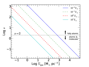
Figure 1 shows how the transition from fully atomic to atomic & molecular phase for different metallicities. The value is the minimum complex size required for the transition from atomic to molecular gas for any given metallicity. This represents the need for the gas cloud to be sufficiently large to form . The external UV radiation is first absorbed by dust, which is essentially traced by the metallicity, then by a thin molecular region. If the cloud is too small, then there will not be enough surrounding material to absorb all the UV photons, and the -core will be dissociated. If the cloud is large, we expect a large molecular core. Higher metal content effectively absorbs more radiation, allowing for the formation of at lower surface densities.
Knowing allows us to modify our SF model by replacing in Equation (1) with the mass density . We also change our SF time-scale to a more physically realistic value, namely the free-fall-time of the gas available to form stars
| (13) |
Here, it may be more correct to use as apposed to in Equation 13. In the case where for instance, we are representing a physical situation where most of the mass is in Hi and there is a small molecular cloud. The molecular gas here will be at lower temperatures than the atomic gas with an internal volume density larger than what we would obtain via . In general, the internal volume density of the molecular cloud is greater than or equal to , but to what degree depends highly on internal processes that we cannot model in our current simulations, such as the internal velocity dispersion of the cloud and the molecular cloud virial ratio (M. Krumholz, private communication). In practice this choice does not matter very much anyway, because the bulk of star formation will occur in particles with for either choice. We have performed additional simulations to examine the difference between using or in the denominator of Equation 13, and have confirmed that the differences are insignificant for the results presented in this paper.
Furthermore, observations have shown that SF is a slow process and that the efficiency at which dense regions produce stars is 1% (Krumholz & Tan, 2007; Lada et al., 2010). To account for this we introduce an efficiency parameter of which leads us to our new formulation of Equation (1):
| (14) |
If a gas particle has , then it is eligible to form stars at the above rate.
2.2.2 Assumption on the neutral fraction
As discussed in the previous section, in order to calculate the fractional abundance, we must first calculate the scale-height of Hi, which then allows for the calculation of . Our GADGET-3 code tracks the neutral fraction of each gas particle individually. For the high density multiphase gas however, the neutral fraction is tracked only for the hot phase, and the cold gas fraction is computed within the multiphase ISM sub-particle model (Springel & Hernquist, 2003). For the very high-density particles, most of the mass is in cold, neutral phase (), but the tenuous hot phase determines the temperature.We calculate the neutral fraction using the -parameter for high-density particles above the SF threshold for our N144L10 fiducial run at , and find all of particles to have , and 98% of the hydrogen mass to have . Given the small mass fraction of ionized gas, it is a good approximation to assume that any gas particle with cm-3 (Choi & Nagamine, 2010) is completely neutral () for the scale-height and column density calculations detailed in Section 2.2.1.
2.2.3 formation threshold density and Wind model modifications
This new SF model (Eq. [14]) allows us to compute the density threshold () for individual particles based on their metallicity, above which results in the formation of . In the earlier version of our GADGET-3 code, Choi & Nagamine (2011) implemented the “Multi-component Variable Velocity” wind model, in which a particle was allowed to travel as a wind particle with no hydrodynamic forces applied as long as its physical density exceeded . The wind velocity of each particle was calculated based on the SFR of the galaxy that the particle belongs to. We can now revise this wind criteria to be based off of an individual particle’s formation threshold rather than a fixed value as in previous SF models.
The formation of requires sufficient shielding, or else the molecule will be dissociated by UV radiation. We can set the threshold for formation for each particle by solving Equation (11) for using ; this value allows us to calculate the minimum for SF within our model:
| (15) |
We can then convert this surface density threshold to a volume density threshold using Equation (9) for each particle, which leads us to the minimum volume density required to form H2 at that particle’s particular metallicity:
| (16) |
In other words, this is the formation density threshold. In the present work, if the physical density of a gas particle is above its particular adaptive formation threshold , then it is eligible to be a member of the wind. This minor modification is necessary as it allows the wind formation criteria to adapt to the new SF model. It is a natural consequence based on the assumption that the galactic outflows result from SF, but we will investigate its implication further in the future using higher resolution zoom or isolated galaxy simulations.
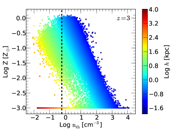
Figure 2 shows the values of vs. metallicity of each particle in a low resolution simulation (N144L10). The previous SF density threshold is shown as the black dashed vertical line. Generally, the values of are higher for each particle than in the previous SF models, allowing for particles to reach higher densities before becoming eligible to form stars. This makes SF in the model less efficient than in the previous SF models. This plot also shows that for a given metallicity, a lower returns higher . Particles with higher metal content have lower formation thresholds due to their ability to absorb more dissociating photons. The accumulation of particles at corresponds to those that have yet to be enriched by SF, but they have varying due to variations in . Some particles at have already been enriched by .
2.2.4 Metal Floor
In our Fiducial runs, initially all gas particles are metal free. Enrichment occurs during star formation; in this process SN explosions return a metal mass of to the ISM, where is the yield, and is the mass of newly formed long-lived stars. It is assumed that each gas particle behaves as a closed box locally, wherein metals are instantaneously mixed between cold clouds and ambient hot gas.
Within the framework of our new SF model, stars can only form if they contain , as determined by Equation (6). In order for , the gas particle must have some metal content. To begin forming stars, we must first enrich the gas particles by hand at very high redshift. Recent high resolution numerical studies by Wise et al. (2012) found that a single pair-instability supernova of a Pop-III or very early Pop-II () star can enrich its host halo to a metallicity of . Their findings are in agreement with observed DLA metallicities, which have metal floors of the same order (Wolfe et al., 2005; Penprase et al., 2010). To mimic this enrichment, we introduce a metal floor of for all gas particles at a specified epoch.
To test the impact of the assumed metal floor, a few low resolution simulations (N144L10) are performed introducing the metal floor at redshifts of , &13; we refer to these as MF9, MF11, & MF13 runs, respectively. The cosmic SFRD histories are nearly identical between these three simulations; they differ only in the point at which each simulation starts to form stars. This is due to the different times at which their metal floors are introduced. The MF11 & MF13 runs both start to form stars at , while MF9 does not begin star formation until . After their initial bursts of star formation, each of the three simulations begin following the same SFRD track from to . The GSMF between the three simulations are also nearly identical at & 6, suggesting that the formation of galaxies within our simulations does not heavily depend on when the metal floor is set. Lastly, the SHMR (cf. Section 3.1.2) is examined at & 6 for each simulation. We find significant scatter in the results for all three runs, but the median SHMR values for each simulation are all well within one standard deviation of one another. This again suggests that the stellar fraction of each halo does not depend heavily on the time at which the metal floor is set.
The redshift at which the metal floor is introduced is related to the metal enrichment by Pop-III and very early Pop-II stars. Since the aim of the current simulations is not to study galaxy evolution at , we choose to introduce our metal floor at the epoch of reionization. Observational estimates by Komatsu et al. (2011) suggest this happens at redshift . In our simulation, reionization is set by the UV background model (Faucher-Giguère et al., 2009, December 2011 version)111https://www.cfa.harvard.edu/~cgiguere/UVB.html, hence our metal floor of is set at accordingly.
2.3. Gas phase diagram
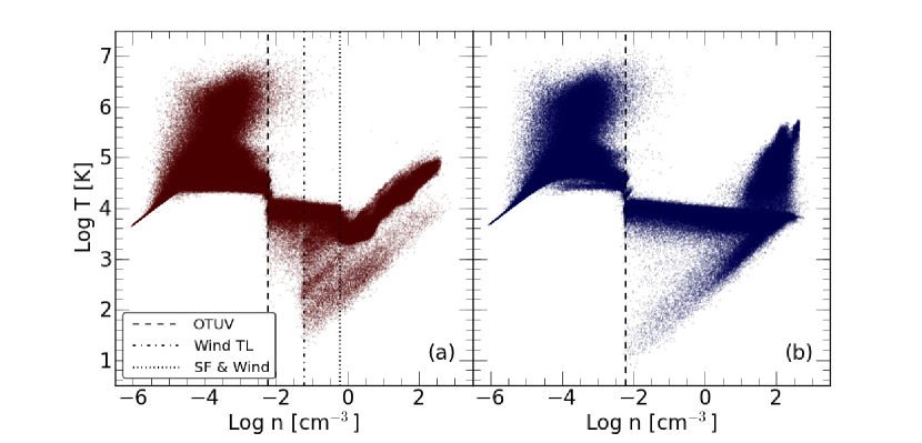
We examine a low resolution N144L10 simulation to study the gas temperature-density phase diagram. Figure 3 compares our Fiducial run with the new run at . Panel (a) represents our Fiducial run and contains three vertical lines representing different thresholds. The left most dashed line ( cm-3) represents an optically-thick ultra-violet threshold or ‘OTUV’ (Nagamine et al., 2010). Any particle below this threshold will be heated by the UVB to K; any particle above this threshold is shielded from the UVB. Nagamine et al. (2010) and Yajima et al. (2012) have demonstrated that this threshold is reasonable using full radiative transfer calculations.
The right most dotted line in Figure 3a represents the constant SF physical density threshold ( cm-3) in the Fiducial run. Any particle whose density exceeds this threshold is allowed to form stars based on the prescription outlined in Section 2.1.2. At densities & temperatures above cm-3 & K, we begin to see the effects of SN feedback and the multi-phase ISM model (Springel & Hernquist, 2003). The cold phase component dominates the mass of the particle, but the hot phase governs the temperature. What is seen in this ‘arm’ is the temperature of the gas heated by SN feedback (hot phase component), and the density of the cold phase component. When we direct our attention to the run (Panel b) we see that this arm is now extended out to higher densities at lower temperatures. This is because stars are only allowed to form if the gas particles contain any above the adaptive density threshold given by Equation (16). As discussed earlier, Figure 2 illustrates how is typically higher than the previous SF density threshold, which allows particles to condense to higher densities without being heated by SN feedback.
The dot-dashed line in between the two previously discussed lines in Figure 3a represents the maximum wind travel length (TL) threshold of cm-3. If a particle becomes a member of the wind, hydrodynamic forces are turned off for a brief period of time (Springel & Hernquist, 2003; Choi & Nagamine, 2011). This allows the gas to adiabatically expand and cool to lower temperatures until the density drops below , or the brief period of time has elapsed. The dot-dashed line is absent from the Panel (b) because of the varying density threshold for each particle. Instead of a temperature discontinuity, as can be seen in Panel (a), we have a ‘tail’ that extends all the way to the OTUV threshold. This tail corresponds to wind particles that have adiabatically expanded as part of the galactic wind.
2.4. Atomic to molecular transition
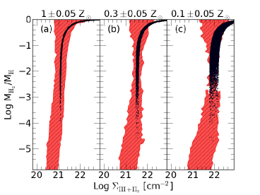
It is important to study where the atomic to molecular transition occurs in our simulations. Figure 4 shows this transition as a function of gas surface density in our N600L100 run at for three different metallicity ranges. In the KMT model, the value of is solely determined by the surface density of gas and metallicity (Equations 6, 11 & 12), therefore the simulation data (black dots) in all three panels is restricted to a relatively thin band determined by the range of metallicity chosen.
Christensen et al. (2012) examined this transition for three isolated Milky Way-like simulations at different metallicities to test their fully time-dependent, non-equilibrium calculation. Their raw simulation output can be seen as the red contour in Figure 4. The transition in our simulations is in good agreement with theirs, corroborating the comparison work of Krumholz & Gnedin (2011). However, our data deviates to higher column densities at high molecular fractions due to the per-particle overestimation of the column density calculated by the Sobolev-like approximation, as discussed in Section 2.2. This deviation should not pose a problem since particles in these high column density regions are already primarily molecular.
3. Results on galaxy populations
3.1. Dark matter halo content
Dark matter (DM) particles were grouped using a simplified version of the parallel friends-of-friends group finder SUBFIND (Springel et al., 2001). The code groups the particles into DM halos if they lie within a specified linking length. We adopt a standard value of for the linking length parameter, which is a fraction of the initial mean inter-particle separation. Each halo must also have a minimum of particles to be considered a halo.
The DM halo mass functions were found to be in agreement between the and Fiducial runs. This is an expected result, because both sets of simulations were started from identical ICs. Both results are in good agreement with the Sheth & Tormen (1999) mass function. This paper focuses on baryonic properties, and it is useful to examine and compare the contents of these halos between the Fiducial and runs. The contents of each halo are calculated by the summation of particle properties located within (Mo & White, 2002) of each halo’s center of mass.
3.1.1 Baryon fraction
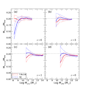
Figure 5 presents the baryon mass fraction over halo mass ()/) as a function of at & 0. Here the cosmic mean () is illustrated by the horizontal black dashed line. Panel (a) shows the composite data from the N400L10, N400L34, & N600L100 runs at ; Panel (b) is composite data from the N400L34 & N600L100 runs at ; Panels (c) & (d) are composed of data from the N600L100 simulation only at and 0, respectively. Solid lines represent the median value within each bin, and the hatched regions represent a 1 spread in the data. The cutoff of the data at lower mass end is determined by the halo mass limit of the halo grouping.
At (panel [a]), the of the two SF models agree with each other well and with the cosmic mean for halos above . Halos below this mass in the run have lower than in the Fiducial run by %. This is presumably due to the different UVB model between the two runs; in the run the UVB is turned on much earlier, and the gas in low-mass halos are photo-evaporated.
This large difference in is nonexistent in low mass halos at as shown in Panel (b). The median values within the run are now generally higher than those in the Fiducial run. As we will see in later sections, this is likely due to higher SFRs and hence stronger SN feedback in the Fiducial run, and this trend continues to . The scatter in at is greater for the model, but it encompasses that of Fiducial run. Both begin to drop slightly below the cosmic mean at around .
By , in the most massive halos settle to a value that is lower than the cosmic mean by %. Again in Panel (c), we see in massive halos with is in agreement between the two models. At lower , the Fiducial run still shows a lower baryon fraction. Finally at , we see that, for the halos with , the mean has decreased slightly since . This means that the halos on average have acquired more dark matter than baryons (either through mergers or accretion), and/or at the same time lose the gas from galaxies due to SN feedback. The scatter of for lower mass halos is generally greater than for the massive halos, and this is a known resolution effect (e.g., O’Shea et al., 2005).
3.1.2 Stellar-to-halo mass ratio (SHMR)
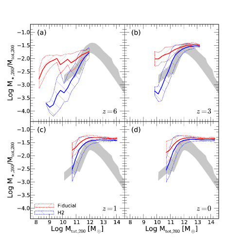
The ratio of stellar-to-halo mass as a function of total halo mass (DM+gas+stars within ) provides a useful insight on the efficiency of star formation in different halos, and it has collected significant attention in the recent years (Conroy et al., 2007; Baldry et al., 2008; Behroozi et al., 2010; Moster et al., 2010; Foucaud et al., 2010; Evoli et al., 2011; Leauthaud et al., 2012; Papastergis et al., 2012). All of these work find a prominent peak in this relation at , suggesting that there is a characteristic halo mass that galaxy formation is most efficient. This mass-scale roughly corresponds to the characteristic stellar mass of GSMF, i.e., the knee of Schechter function, where most of the stellar mass has formed globally. To further surprise, Behroozi et al. (2013, hereafter B12) found that, using observational data and semi-analytic modeling, SHMR is almost time-independent between to . This is interesting, because SHMR should reflect all the cumulative effects of past star formation and feedback, and a non-evolving SHMR suggests tight self-regulation and a subtle balance between star formation and feedback. It is a significant challenge for any cosmological hydrodynamic simulation to reproduce this relation across a wide range of halo mass and cosmic time.
Note that we are specifically using , and not for this comparison. This is because Munshi et al. (2013) pointed out that, in order to accurately compare simulations to semi-analytic model results (such as abundance matching technique), one must observe the simulations in a similar manner. They refer to the work by Sawala et al. (2013), who showed that in -body simulations can be greater than those in -body+hydro simulations by up to , because various baryonic processes (gas pressure, reionisation, supernova feedback, stripping, and truncated accretion) can remove baryons from the halo, decreasing the total mass systematically. Additionally, Graham et al. (2005) found that the stellar mass component of observed galaxies could be systematically underestimated by in some cases; for example, additional flux of 0.22 mag lies beyond the SDSS Petrosian aperture for a galaxy that has an profile. Here, we consider that it would be more natural to examine SHMR as a function of rather than correcting our results by a certain number.
In Figure 6, we show the SHMR in our simulations by calculating the total stellar mass contained within of each halo’s center-of-mass (). If we assume that the B12 data extends out to , we see in Figure 6a that our run does a good job at reproducing the B12 data at , much better than the Fiducial model. We have verified that the different UVB models do not impact this result. The comparison of the models in Figure 6 clearly suggests that the suppression of star formation in low-mass halos is favorably achieved by the model. Note that this SF suppression is not due to the SN feedback, but rather due to the metallicity dependence of the new -based SF model. This could become a critical point to distinguish between the -based and turbulence-based SF models in the future.
At (Figure 6b) the SHMR increases slightly for both simulations. Our simulations are in agreement with the B12 data at . However, we continue to overestimate SHMR at down to , which could be due to lack of AGN feedback in our current simulations. It is widely believed that both thermal and momentum feedback from supermassive black holes suppresses the star formation in massive halos, making them ‘red & dead’ (e.g., Di Matteo et al., 2005; Springel et al., 2005; Nagamine et al., 2005; Ostriker et al., 2010; Choi et al., 2012). There is little evolution between & 0 in our simulations (Figure 6c,d), and our results are higher than B12 data even for low-mass halos at .
3.2. Quantities related to star formation
3.2.1 Cosmic star formation history
With the model producing less stars in lower mass halos, we expect the cosmic SFRD to be lower as well. When comparing simulations to observational estimates of SFRD, we have to be careful about which IMF is being used. The Fiducial and runs use different IMFs. In order to fairly compare the two, we must make corrections to either the simulation data or the observations. Because SFR is a raw output of our simulation, we prefer to take the latter route and correct the observational data to the same IMF as in simulation. A simple factor allows for this conversion:
| (17) |
where represent an arbitrary IMF. To convert from Salpeter to Chabrier, we take (e.g., Nagamine et al., 2006; Raue & Meyer, 2012), and from Salpeter to Kroupa we take (Horiuchi et al., 2009). This is because, for a given amount of observed rest-frame UV flux, the required SFR would be lower for an IMF that is weighted more towards higher masses. After correcting our IMFs, we find that both simulations roughly agree with the observed data.
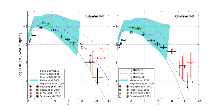
Figure 7 shows the cosmic SFRD history as a function of redshift. As expected, the runs show significantly lower SFRD at most redshifts relative to the corresponding Fiducial runs. The runs do not start forming stars until , which is a consequence of our model. In the run, in order for gas to be eligible for SF, it must first contain , which requires non-zero metal content. As discussed in Section 2.2.4, we introduce the metal floor by hand at , after which stars are able to form. Until the metal floor is introduced, the gas continues to condense to higher densities.
The slopes of the SFRDs at high- are slightly steeper than the Fiducial runs, because the run starts SF a little later than the Fiducial run, and has more abundant high-density gas available for SF. It tries to catch up to the Fiducial run after the metal floor is introduced. For the same reason, the peak of the SFRD of the N600L100 run is slightly shifted towards lower redshift compared to the Fiducial run. With a lower SFRD in the runs, there is more gas available for SF at later times.
Note that Figure 7 is only showing the results of different simulations as separate lines, and it does not show the expected total SFRD. To really obtain the total SFRD, we must carefully examine the contribution from each galaxy mass ranges to SFRD, and sum up the contribution from each simulation. This was done by Choi & Nagamine (2010) for the Fiducial runs, and we will present such analyses separately (Jaacks et al., 2013). Here, we simply note that the expected total SFRD would be even higher than the red dot-dashed line of N400L10 run, and it would go right through the data range shown by the cyan and magenta shaded regions.
3.2.2 In which halos do galaxies sit?
So far, we have not considered the grouping of galaxies themselves (i.e., star and gas particles). To examine individual galaxies in our simulations, we group gas and star particles based on the baryonic density field rather than the dark matter. This allows us to identify galaxies directly, and then calculate properties such as their SFRs, stellar masses (, which we distinguish from ), gas masses (, which we distinguish from ) and metallicities. A more detailed description of this galaxy group finding process can be found in Nagamine et al. (2004c).
Together with the friends-of-friends halo finding, we are interested in how the grouped galaxies relate to the DM halos. To find out the matching between the two sets, we search for the nearest DM halo from the center-of-mass of each galaxy. We limit our galaxy sample to those with minimum 10 star particles, and those that reside in halos with at least 100 DM particles. Note that the DM structure between the Fiducial and runs are nearly identical, because they both use identical ICs.
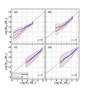
We can then make a scatter plot of corresponding and of each halo as shown in Figure 8. In Panel (a) we see that the low mass galaxies () at in the two runs reside in different halos with different masses; the median result of the two runs lie almost an order of magnitude apart, with the Fiducial run galaxies residing in lower mass halos on average. This is because the SF requires a higher threshold density in the run and the gas requires a deeper potential-well of massive halos in order to form the same amount of stars as in the Fiducial run. The results of the two runs converge at higher masses (), suggesting that those halos contain similar galaxies in the two runs. For higher mass halos with , there seems to be little difference in the SF between the two runs.
This relation does not evolve significantly as time proceeds. For comparison, the dashed lines in Figure 8 represent the same scaling of . The figure shows that the halos grow in mass with time, and the median lines slide up to top-right direction along the dashed line.
3.2.3 Gas mass fraction of simulated galaxies
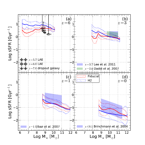
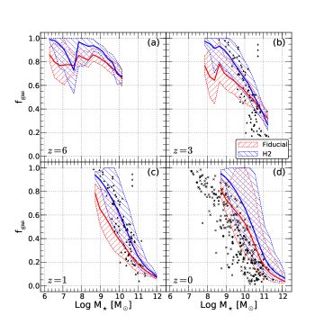
Figure 9 shows the median gas fraction () of simulated galaxies as a function of galaxy stellar mass. In general, in the run is higher than that in the Fiducial run, but the 1 regions overlap with each other. The non-smoothness in the median lines in Panels (a) & (b) are simply due to the procedure of combining data from multiple simulations of different resolutions.
We find that the median lines do not evolve very much over time. At , declines steeply with ; from values close to unity at to at . This suggests that the massive galaxies with in our simulations have converted most of their baryons into stars, and not much gas is left in them, coinciding with the downturn of the SFRD at these epochs (Figure 7).
Black triangles in Panels (b) & (c) are from a sample of galaxies at (Erb et al., 2006). Simulated galaxies from the run tend to agree better with the observed data at . In Panel (d) we show observational data of nearby galaxies from McGaugh (2005, stars), Leroy et al. (2008, filled circles), and West et al. (2009, 2010, crosses). Neither the or Fiducial models agree well with observations at . This may in part be due to the limited mass resolution of the N600L100 run; a higher resolution run would resolve lower mass galaxies, possibly shifting the distribution to the left in better agreement with observations, if we were to make a composite plot from different runs. Another possible cause for this discrepancy is that too much unenriched gas has fallen into these massive galaxies between and , pushing to higher values.
3.2.4 Specific star formation rates of galaxies
Figure 10 shows the redshift evolution of the specific star formation rates (i.e., SFR per unit stellar mass, ) in our simulations. This plot shows the instantaneous efficiency of SF, whereas the SHMR reflects all past history of SF and feedback. Panel (a) shows that the low mass galaxies in the run at have higher sSFRs than those in the Fiducial runs, mirroring the steeper slope of the SFRD (Figure 7) for the run. Our simulation data is higher than the observational data of Lyman- emitters at & 6.6 (Ono et al., 2010) and -dropout galaxies at (Labbé et al., 2010b), but within their error bars.
The run in Panel (b) () again show a slightly higher sSFR than the Fiducial run for lower mass galaxies with . At higher masses, the two runs agree very well, as well as with the observed data at & 2.0, indicated by the shaded region (Daddi et al., 2007; Lee et al., 2011). Panel (c) () also shows similarly good agreement between the two runs and the observational data range (Elbaz et al., 2007).
Panel (d) () shows that the sSFR of both runs continue to decrease with time, but the run decreases at a faster rate. Therefore the Fiducial run has a higher sSFR than the model at . Both models agree with the observational data (Brinchmann et al., 2004) with a slightly decreasing sSFRD as a function of .
3.2.5 Redshift evolution of the sSFR
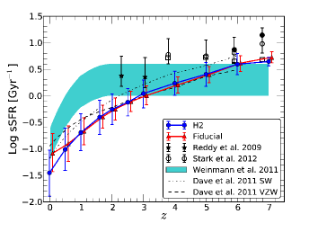
Observations indicate that galaxies of similar mass () have relatively constant sSFRs on the order of in the redshift range of (e.g., Stark et al., 2009; González et al., 2010; Labbé et al., 2010b, a). This sSFR ‘plateau’ is difficult to produce with current models of galaxy formation (e.g., Bouché et al., 2010; Weinmann et al., 2011). Figure 11 shows the sSFR as a function of redshift for simulated galaxies with . We find that the sSFR for these galaxies decline gradually rather than a steep drop off around as observations suggest. The run however, produces a slightly steeper drop off at than the Fiducial run, but the normalization is still lower than the compilation of observed data points by Weinmann et al. (2011). Neither model produces the observed plateau in the redshift range of .
For comparison, simulation data from two different wind models of Davé et al. (2011, dashed & dot dashed lines) are included, and they show similar trends to our simulation data. Our results are also very similar to the results of the semi-analytic model of Neistein & Weinmann (2010); Weinmann et al. (2011) without the plateau at . The general agreement between multiple different simulations and semi-analytic models of galaxy formation suggest that the CDM model predicts a general decline in the sSFR of galaxies of a given mass, contrary to observations. However, we note that none of these simulations included the effect of AGN feedback. Krumholz & Dekel (2012) argued that taking the metallicity-dependence of formation would help to reconcile the discrepancy, however, even with our new -based SF model, our simulations do not produce the plateau of sSFR at .
3.3. Galaxy stellar mass function (GSMF)
In the previous sections, we have seen that SF is less efficient in the run, which should also be reflected in the GSMF. Recall that for a given at high-, the galaxies reside in more massive halos in the runs (Figure 8). Since the higher mass halos are less abundant in a CDM universe, this will reduce the number of low-mass galaxies and shifts the galaxy population to higher mass DM halos.
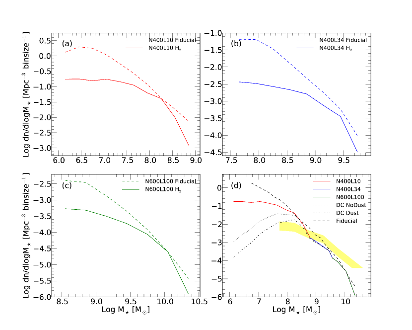
Figure 12 shows the GSMF for our three primary runs (N400L10, N400L34, N600L100) at . In Panels (a-c) we directly compare the run to the corresponding Fiducial run for each simulation, and find that the run produces far fewer low-mass galaxies as expected. Note the different y-axis ranges in Panels (a-c). Our result is in general agreement with the findings of Kuhlen et al. (2012); they also found a decrease in their GSMF at at .
Figure 12d shows the comparison of the composite GSMF from the two runs, following the method of Jaacks et al. (2012a); we connect the GSMF from runs with different box sizes at the resolution limit of each run. This method allows us to cover a wider range of utilizing many simulations, and present the results collectively. The observational estimate from González et al. (2010, yellow shade) at is also shown. At the high-mass end of , the two composite GSMFs from and Fiducial runs agree well. The slight kink in the composite GSMF at for the run is due to the resolution gap between the simulations; we have verified that an intermediate resolution run (N500L34, ) fills in this gap. Due to the heavy computational load, we did not complete the corresponding Fiducial run for N500L34, therefore this run is not used for other comparisons in this paper. At the low-mass end of , the run has a significantly lower number density of galaxies than the Fiducial run. This illustrates that the model has a greater impact on the number density of low-mass galaxies.
3.3.1 On the over prediction of GSMF at high-
One of the primary motivations for implementing the -based SF model was to see if it can remedy the overprediction of GSMF at low-mass end due to its natural dependence on metallicity as we described in Section 1. In the earlier sections, we saw that indeed the -based SF model reduces the number of low-mass galaxies. However, even with the new model, we are still over-predicting the number of low-mass objects at compared to the observational estimate of González et al. (2010) at (Panel [d]). Therefore the model alone does not seem to be able to solve this generic problem of CDM model. Our simulations also seem to under-predict the number of massive galaxies with when compared to the González et al. (2010) observational data at . Jaacks et al. (2012a) argued that this difference likely originates from the different slope in the SFR relation, where the observational estimate was derived by using a crude relation from and applied to assuming that it is unchanged. In our simulations, the SFR relation has a different slope, and this results in a different slope in the GSMF.
Figure 12d also contains the results of applying the duty cycle (DC) corrections (Jaacks et al., 2012b) to our composite GSMF both with (dot-dashed line) and without (dotted line) accounting for dust extinction. Jaacks et al. (2012b) defined the DC as the fraction of time that a galaxy exceeds the current HST magnitude limit within a certain , and characterized it with a sigmoid function as a function of . According to their result, DC for makes a relatively sharp transition from nearly zero at , crosses 0.5 at , and to almost unity at . Using this relation, we can apply a correction for the observability of low-mass galaxies, and see the impact of SF duty cycle on the observed GSMF. Similarly to the results of Jaacks et al. (2012b), our GSMF becomes closer to the observational estimate after the DC correction. This comparison demonstrates that the -SF model alleviates some of the tension between observation and simulation without having to invoke stronger stellar feedback prescriptions.
3.3.2 GSMF at and 0
Figure 13 shows the GSMF at (Panel a) & (Panel b). Panel (a) is composed of data from the N400L34 & N600L100 runs, and Panel (b) of N600L100 data. Dashed lines represent the Fiducial run, while solid lines represent the run. The shaded regions at represent observational estimates of the GSMF at (yellow) and (cyan) from Marchesini et al. (2009), following Choi & Nagamine (2010). Both sets of simulations are in agreement with each other and with observations at , which corresponds to (Figure 8b). A substantial difference between the two SF models is again seen in galaxies with , but this is below the current observable flux limit.
We may try to understand the discrepancies in the GSMF in relation to the SHMR. The difficulty is that the SHMR is not per unit volume, hence there is no obvious direct link between SHMR and GSMF. Suppose in low-mass halos is increased uniformly, then the normalization of SHMR shifts upwards. At the same time, those galaxies would move from the low-mass bin to higher mass bins, and the GSMF would be weighted more towards higher mass side. For example, Figure 6b suggests that we are producing roughly correct amount of stars in halos with at , and the agreement in the GSMF is not so bad either as shown in Figure 13a. Such a comparison provides a consistency check between SHMR and GSMF.
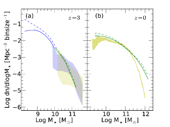
The shaded region at (Panel [b]) is the observational estimate from Cole et al. (2001). Our simulations agree well with the observation near the knee of GSMF (), but over-predicts at both low and high mass end. This over-estimation at is reflected in the overestimation of the SHMR at (Figure 6d), which could be due to a lack of AGN feedback in our current simulations. At the low-mass end (), both models over-predict the GSMF, but the run to a lesser degree.
It is clear that simultaneously matching the SHMR and GSMF is not an easy task. We expect the inclusion of AGN feedback will assist in improving the high-mass end of our simulations at low redshift. The new -based SF model seems to have improved the relations in regards to the low-mass end, but does not fully reconcile the differences. Further improvements to our SN feedback prescriptions (e.g., momentum feedback by winds) may be required to achieve better agreement with observations.
3.4. Kennicutt-Schmidt (KS) relationship
Ideally we would like to reproduce the empirical Kennicutt-Schmidt relationship naturally in simulations; previously the KS relation was imposed in our SF prescription (Choi & Nagamine, 2010) and in many others’, therefore the results matched the observation well by construction. The new -based SF model provides two main benefits: it is not ‘tweaked’ to match the KS relation, and it is more physically realized in that stars are formed out of cold molecular gas on a depletion time-scale which is equal to about 1% of the free-fall time (i.e., with 1% efficiency per free-fall time).
To examine the KS relation, we calculate the column density of Hi, , and SFRs along the z-axis of each halo in our simulation on a uniform grid with a cell size of . A detailed description of this process can be found in Nagamine et al. (2004a). In Section 2.2, we stated that the model was accurate for , yet we set our metal floor below that at . The model fails at low metallicities by over-predicting the amount of mass. This is due to time-dependent effects being neglected within the analytical KMT model (Krumholz & Gnedin, 2011). However, the over-predicted value may be an accurate estimate of how much cold material is present to form stars (Krumholz, 2012). Therefore we simply assume that the value calculated by Equation (6) for any gas particle with is actually representative of the amount of cold Hi gas, which is available for star formation.
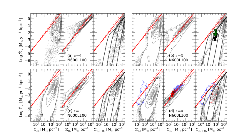
Figure 14(a-d) shows the KS relation for the N600L100 simulation at , & 0. Each point in this figure represents one pixel on the projected x-y plane, and the contour is used to represent all the columns from all halos in the simulation box. For each redshift, the panel is broken down into three sub-panels: the first being the KS relation for Hi gas only, second is for gas only, and lastly for Hi +. We will refer to these panels as KS-HI, KS-H2, and KS-HIH2, respectively. Each panel includes the KS relation given by Equation (3) as a solid red line, with the dashed lines representing the range of slope .
In KS-HI panel at , we also overplot the observational data from seven nearby spiral galaxies as a blue hatched region (Bigiel et al., 2008, hereafter B08). In KS-H2 panel (), we overplot the low surface density observations from the Small Magellanic Cloud (SMC) as red triangles (Bolatto et al., 2011, hereafter known as B11). Lastly in KS-HIH2 panel (), we again plot B08 data as a blue hatched region, and B11 data from the SMC as a red hatched region.
There are two major processes driving the evolution of these plots. The first is gas depletion: as time passes the cold molecular gas used to form stars is depleted, and become less available at late times. This is most obvious in the decrease of between , corresponding to the downturn of the SFRD at in Figure 7. The second is metal enrichment: the longer a simulation runs, the more enriched the gas becomes via SF. This process expands the distribution of points to the left-hand-side of the plot, because higher metal content allows stars to form at lower surface densities, as shown in Figure 1. The distribution of points broadens from to , indicating greater range of metallicities present in the simulations.
The KS-HIH2 panels include theoretical results from the KMT model (Krumholz et al., 2009) to show the same effect. The column densities calculated for each pixel represent the smoothed value on a relatively large projected scale of ; if we use this value, the model will underpredict , since it does not account for clumping of the gas on scales below our simulation’s spatial resolution limit of , as well as the path-length along the column. To account for this effect, the KMT model multiplies the calculated gas column density by a clumping factor “” (), which increases the surface densities to be compared with observations. In order to compare the KMT model result with our simulation, the theory lines are shifted to lower ‘computed’ surface densities (i.e., ), which brings a good agreement between the KMT model results and our simulations. In Figure 14, we adopted .
For the KS-HI panel at , we find disagreement between simulation and the B08 data (blue hatched region). This is a metallicity effect; our simulations do not contain enough high-metallicity columns, and the low metallicity columns will form stars at higher surface densities in the KMT model.
In the KS-H2 panel at , our simulation is in good agreement with the observations. The starts high at , and eases its way to the lower left due to the two processes described above. By , the observations lie in the center of our simulation data showing a very good agreement even for low surface densities. It should be noted that we are directly measuring the amount of in our simulation, whereas the observers infer this value from the CO luminosity.
In the KS-HIH2 panel at , we again find a disagreement between simulation and the B08 data (blue hatched region); the bulk of our data is found at slightly higher surface densities compared to these observations. The data in these panels is dominated by Hi, resulting in similar trends to the KS-HI panel.
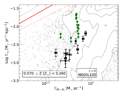
In the KS-HIH2 panel at (Panel [b]), we also overlay the upper limits from damped Lyman-alpha absorbers (DLAs) as green circles and outskirts of Lyman-break galaxies (LBGs) as black squares (Wolfe & Chen, 2006; Rafelski et al., 2011). LBGs are considered to be star-forming galaxies with moderate median mass of , therefore are expected to have been enriched to some level. Rafelski et al. (2011) find the LBGs in their sample have . Figure 15 shows the KS plot for only star-forming columns in our N600L100 simulation with at . The observed data points are close to the edge of the simulation contour, but there are many columns that agree with the observational data. Note that it is certainly easier to observe the SFR closer to the upper edge of the contour rather than the bottom side of it due to the surface brightness dimming.
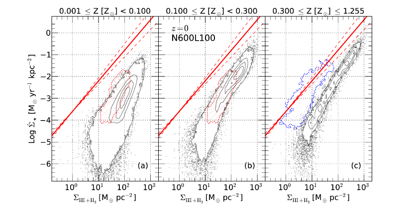
Figure 16 further illustrates the metallicity effect by separating the KS-HIH2 panel from Figure 14d into three different metallicity ranges for the N600L100 run at . We find that the columns with the lowest metallicity (Panel [a]) are forming stars at the highest gas surface densities for a given as expected. Panel (b) brackets , which is roughly equal to the metallicity of the SMC (Bolatto et al., 2011). Columns in our simulation in this metallicity range agree very well with the observed data (red contour). In Panel (c) we show columns of higher metallicity , which is similar to the range of B08 sample () (Walter et al., 2008). As discussed previously, our data does not agree very well with observations in this range. There are some points overlapping with the observed data, but the majority lie at higher column densities than the observed range. This discrepancy is presumably caused by different metallicities: the highest metal column at in the N600L100 run is , yet the median column metallicity at is . This suggests that our N600L100 run does not contain enough high metallicity columns to match these observations. If the simulation had more high metallicity columns, then the SF would occur more at lower gas surface density, and there would be more points overlapping with the B08 data. This discrepancy could be related to our SN feedback and galactic wind models since the metal recycling process is tightly connected with them.
3.5. Hi & H2 column density distribution functions
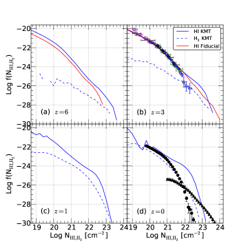
One of the best ways to investigate the distribution of Hi gas in the Universe statistically is to examine the Hi column density distribution function (e.g., Nagamine et al., 2004b, a; Wolfe et al., 2005; Zwaan & Prochaska, 2006; Prochaska & Wolfe, 2009; Noterdaeme et al., 2009; Pontzen et al., 2010; Altay et al., 2011; Yajima et al., 2012; Rahmati et al., 2013; Erkal et al., 2012; Noterdaeme et al., 2012). Using the Fiducial runs, Nagamine et al. (2010) found that a simple self-shielding model with a threshold density ( cm-3) for UVB penetration can reproduce the observed quite well at for . Yajima et al. (2012) later showed the validity of value using full radiative transfer calculations. However, Nagamine et al. (2010) also found that the Fiducial run over-predicts at , and argued that this might be due to the neglect of within the Pressure SF model (Section 2.1.2), because then part of Hi would be converted into and would decrease at high values.
Figure 17 compares the column density distributions of both Hi and in the and Fiducial runs at . Panels (a) & (b) are composed of N144L10 data, while Panels (c) & (d) are composed of N600L100 data. The Fiducial run is omitted from panels (c) & (d), because the N600L100 Fiducial run did not use the OTUV threshold which is necessary to bring the column density distribution into agreement with observations at (Nagamine et al., 2010).
In Panel (a) we see that the run consistently has higher amplitude of than the Fiducial run due to less efficient star formation. At (b) however, we find that the run has a higher than that of Fiducial run at . This is because the star formation is less efficient in the new run, therefore more Hi gas is left over in high density regions. In the run the varying SF threshold density was higher than the constant adopted in the Fiducial run (Figure 2), and it was also clear from Figure 3 that the gas particles are reaching higher densities in the run before being heated by SN feedback than in the Fiducial run. The results at the lower do not change between the two runs at this redshift. Panels (c) & (d) continue to show the redshift evolution of this relationship in our simulations. At , we find that our simulations over-predict at , over-predict the at , and under-predict at .
Therefore the current simulations suggest that it is difficult to explain the sharp turn-down of observed at by the atomic-to-molecular transition, in agreement with the conclusions of Erkal et al. (2012). Additionally, Erkal et al. (2012) showed that their simulations could be brought into agreement with observations if a region of 3 kpc radius around the center of all galaxies was removed. This could be another opportunity for AGN feedback to play an important role: if feedback from super massive black holes can prevent the formation of high columns, then our simulations may come into better agreement with observations at . Obviously more refinement of feedback models are needed to bring the simulations into agreement with the observations of and .
3.6. Resolution studies
The new -based SF model has an implicit resolution dependence. With higher resolution, the simulation resolves higher (column) densities (Eq. 9), which yield lower values (Eq. 11) for a given metallicity. Figure 1 illustrates that lower values lead to higher (Eq. 6), which increases the SFR (Eq. 14).
To examine the resolution effect, Figure 18 shows the KS relation for the N600L10, N400L10, N400L34, & N600L100 runs at . These panels are ordered by resolution: Panel (a) shows the highest resolution, and Panel (d) shows our lowest resolution simulation. In Panels (a) & (b), we can examine the resolution effect on the KS plot when keeping the box size constant. In general the gas surface densities where SF takes place do not change very much, but with higher resolution, the points cover a wider range of . This is an expected result from a higher resolution simulation; the additional resolution allows the gas to collapse to higher densities, yielding additional shielding which eases the transition to .
While Panels (a) & (b) are both from simulations with a box size of comoving Mpc, Panels (c) & (d) are from simulation boxes of and , respectively. Increasing the box size of a simulation usually comes with a price of decreasing the resolution, and it results in more higher mass halos and fewer low-mass halos (e.g., Thompson & Nagamine, 2012). Note that the simulations shown in Panels (c) & (d) are of lower resolution than those in Panels (a) & (b). When comparing the L10 boxes with the L34 & L100 boxes, we are actually examining the resolution and box size effects simultaneously. Comparing all the panels in Figure 18 suggests that our KS results are not significantly affected by these resolution effects. The only visible effect we see in the figure is that the lower resolution results in a thinner contour distribution
3.6.1 Probability Distribution Function (PDF) of density
Physical number densities of observed molecular clouds are on the order of a few hundred cm-3, in rough agreement with the highest densities achieved in our current cosmological simulations. Figure 19 shows the mass-weighted PDF of number density at the highest densities in our simulations at . As expected, we can see that the peak of the highest density region shifts to higher densities as the resolution increases; the lowest resolution production run (N600L100) has a peak at cm-3, and our highest resolution production run (N400L10) has a peak at cm-3. However, the N400L10 run has a slightly different shape from the other runs, and the higher resolution N600L10 run has a peak at a slightly lower value of cm-3. The exact reason for this different PDF shape is unclear, but presumably it was affected by some SF events.
Earlier, Jaacks et al. (2012a) showed that the Fiducial runs do not satisfy the Bate & Burkert (1997) mass resolution criteria, even though gas particles in our N400L10 have particle masses lower than the typical Jeans mass at by a factor of . This prevents us from explicitly resolving the collapse of star forming molecular clouds directly, and it is one of the primary reasons for employing a sub-grid model for SF using the KMT model. Given that the highest densities reached in our simulations is approximately equivalent to those of observed giant molecular clouds, we consider that the KMT is suitable to use as a sub-grid model in our simulation to estimate the mass for star formation. In fact, the KMT model is well suited to predict the galactic-scale trends in atomic and molecular content rather than the structure of individual photo-dissociation regions (Krumholz et al., 2008; Kuhlen et al., 2012).
4. Summary
We have implemented a new -based SF model in our cosmological SPH code GADGET-3 . Previous SF models did not consider the formation of , and imposed the KS relation in their SF prescriptions. The analytic KMT model has provided a computationally inexpensive way to estimate the mass fraction in cosmological hydrodynamic simulations, which allows us to modify our SF prescription to compute the SFR based on density rather than total gas density. The model brings a natural dependence of star formation on metallicity (in addition to the previous dependence through metal line cooling).
We performed a series of cosmological simulations with different box sizes and resolutions, and examined how this new -based SF model affected the results such as stellar-to-halo mass ratio, cosmic SFRD, galaxy specific star formation rates, galaxy stellar mass function, Kennicutt-Schmidt relationship, and Hi & column density distributions.We find that this new -based SF model provides many advantages over previous models, and we summarize our primary conclusions below.
-
•
In the new -based model, each gas particle has different SF threshold densities based on its metallicity (Figure 2). We have shown that the new SF threshold densities (i.e., metallicity-dependent density required for formation) are higher than the constant threshold density used in the Fiducial run, which results in overall decrease of SFRD (Figure 7) in the new model. Decrease of star formation leads to weaker feedback effects subsequently. The need for sufficient shielding from radiation field for formation results in lower SFR, causing a gas reservoir to build up. Consequently, SF starts later than in the Fiducial run, and the peak of SFRD has slightly shifted to a lower redshift. But both runs are still compatible with the observed range of SFRD in the Lilly-Madau diagram.
-
•
The run is able to successfully reproduce the SHMR at & 6 for lower mass halos with (Figure 6). The Fiducial run with previous SF model significantly overpredicts SHMR at the same mass range, therefore the run provides a significant improvement on this aspect. Since the SN feedback model was kept the same in the two runs, this improvement was purely driven by the change in the SF model, rather than the feedback.
Both runs overpredict the SHMR in halos at , which might be due to lack of AGN feedback in our current simulations. This is connected with the over-prediction of GSMF at the high-mass end in our simulations.
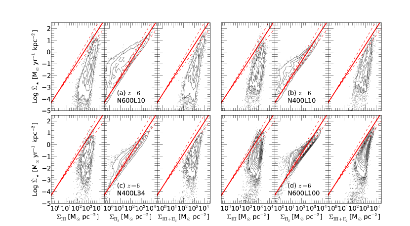
Figure 18.— Similarly to Figure 14, we plot the KS relation for the N600L10, N400L10, N400L34, & N600L100 simulations at to examine the resolution and box size effects. See text for detailed discussions. -
•
The sSFRs of galaxies in the and Fiducial runs are in rough agreement with observations (Figure 10), and they decrease systematically with decreasing redshift. At , the run has a higher sSFR for galaxies with , but this is due to the fact that the galaxies with same reside in higher mass halos in the runs than in the Fiducial run (Figure 8). At later times, this difference becomes much smaller and the two models are in rough agreement with one another.
However, the median sSFR of simulated galaxies with does not behave consistently with the observations as a function of redshift (Figure 11). Both our Fiducial and runs predict gradually declining sSFR with decreasing redshift, similarly to other previous models (Bouché et al., 2010; Davé et al., 2011; Weinmann et al., 2011). Krumholz & Dekel (2012) argued that taking the metallicity-dependence of formation would help to reconcile the discrepancy, however, even with our new -based SF model, our simulations do not produce the plateau of sSFR at . The general agreement between multiple different simulations and semi-analytic models of galaxy formation suggest that the CDM model predicts a general decline in the sSFR of galaxies of a given mass, contrary to observations. However, we note that none of these simulations included the effect of AGN feedback.
-
•
We find that the -based SF model produces significantly fewer galaxies at compared to the Fiducial run at (Figure 12d). Even after this reduction, the faint-end slope of GSMF in the run is still steeper than what has been observationally estimated at . Employing duty cycle corrections following Jaacks et al. (2012b) brings the GSMF closer to observations.
At we find that our simulations are in good agreement with observed GSMFs at , consistent with our previous finding in Choi & Nagamine (2010). At the lower masses of , again the model produces fewer number of low-mass galaxies relative to the Fiducial run. At the moment, the flux limit of GSMF data is even with the deepest HST imaging, and there is no good data below this limit. Galaxies with correspond to halos with , and in this regime the new run agrees with the observational estimate of SHMR much better than the Fiducial run. For this reason, we expect that the run would match the observations of GSMF better in the future at .
Finally at , we find that our simulations over-predict the GSMF at both low and high-mass end. The deviation at the low-mass end seems smaller than at the high-mass end, however, since this is a log-log plot, the actual deviation is greater at the low-mass end. Further improvement in our feedback prescriptions (e.g., momentum-driven feedback by SN and AGN) may be needed to reconcile these differences.
-
•
We find that the new -based SF model naturally produces the empirical Kennicutt-Schmidt relationship without the need for ‘tweaking’ the parameters of the SF model. The most significant discrepancy between the run and observation can be seen against the nearby spiral galaxy data of Bigiel et al. (2008). It seems that the run does not contain enough high-metallicity columns to match observations of nearby spiral galaxies. These discrepancies indicate that our current simulations might have too much low-metallicity gas in massive galaxies at , which is also indicated by Figure 9d. However the run is able to match the observations of DLAs and LBGs at , as well as the observations of the low-metallicity SMC by .
-
•
As for the hydrogen column density distribution function, we find that the new model did not improve the agreement with observation at at , and we still over-predict similarly to the previous simulations. Erkal et al. (2012) also concluded that the atomic-to-molecular transition alone could not account for the downturn in at . At , our simulations do not agree with the observational data of Zwaan & Prochaska (2006), and further refinement of star formation and feedback models are needed.
Finally, it is important to point out that SN feedback and subsequent metal enrichment is tightly coupled with SF within our simulations. We must be mindful of this when comparing to observations, as changing the SF prescription could inherently change the metal enrichment process. While the new -SF model may alleviate some of the discrepancies between simulation and observations, we recognize that the problem is not completely solved. Further improvements to our feedback prescription may be required in order to reach better agreement with observations.
As for our future plan, we intend to improve our simulations on a few fronts, given the problems that we observed in this paper. Since the calculated in the KMT model depends on gas metallicity, we need to account for the metal diffusion in the ISM more accurately (e.g. Shen et al., 2010). Our current SPH code does not allow for particles to share their metal content with one another, and we plan to implement and explore the effects of metal diffusion in the future. Finally, as a comparison to the -SF model, we also plan to develop a turbulence-based SF model and explore the differences between the two approaches to star formation.
Acknowledgements
We are grateful for the helpful and insightful discussions with Mark Krumholz and Brant Robertson. We thank Volker Springel for providing us with the original version of GADGET-3. This work is supported in part by the National Science Foundation (NSF) grant AST-0807491, National Aeronautics and Space Administration (NASA) under Grant/Cooperative Agreement No. NNX08AE57A issued by the Nevada NASA EPSCoR program, and the President’s Infrastructure Award from UNLV. Support for Program number HST-AR-12143.01-A was provided by NASA through a grant from the Space Telescope Science Institute, which is operated by the Association of Universities for Research in Astronomy, Incorporated, under NASA contract NAS5-26555. This research is also supported by the NSF through the TeraGrid resources provided by the Texas Advanced Computing Center (TACC) and the National Institute for Computational Sciences (NICS). KN is grateful to the hospitality and the partial support from the Kavli Institute for Physics and Mathematics of the Universe (IPMU), University of Tokyo, the Aspen Center for Physics, and the NSF grant No. 1066293.
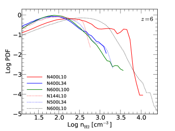
References
- Altay et al. (2011) Altay, G., Theuns, T., Schaye, J., Crighton, N. H. M., & Dalla Vecchia, C. 2011, ApJ, 737, L37
- Baldry et al. (2008) Baldry, I. K., Glazebrook, K., & Driver, S. P. 2008, MNRAS, 388, 945
- Bate & Burkert (1997) Bate, M. R. & Burkert, A. 1997, MNRAS, 288, 1060
- Behroozi et al. (2010) Behroozi, P. S., Conroy, C., & Wechsler, R. H. 2010, ApJ, 717, 379
- Behroozi et al. (2013) Behroozi, P. S., Wechsler, R. H., & Conroy, C. 2013, ApJ, 762, L31
- Bigiel et al. (2008) Bigiel, F., Leroy, A., Walter, F., Brinks, E., de Blok, W. J. G., Madore, B., & Thornley, M. D. 2008, AJ, 136, 2846
- Bolatto et al. (2011) Bolatto, A. D., Leroy, A. K., Jameson, K., Ostriker, E., Gordon, K., Lawton, B., Stanimirović, S., Israel, F. P., et al. 2011, ApJ, 741, 12
- Bouché et al. (2010) Bouché, N., Dekel, A., Genzel, R., Genel, S., Cresci, G., Förster Schreiber, N. M., Shapiro, K. L., Davies, R. I., et al. 2010, ApJ, 718, 1001
- Bouwens et al. (2012) Bouwens, R., Bradley, L., Zitrin, A., Coe, D., Franx, M., Zheng, W., Smit, R., Host, O., et al. 2012, ArXiv e-prints (arXiv:1211.2230)
- Bouwens et al. (2011) Bouwens, R. J., Illingworth, G. D., Oesch, P. A., Labbé, I., Trenti, M., van Dokkum, P., Franx, M., Stiavelli, M., et al. 2011, ApJ, 737, 90
- Brinchmann et al. (2004) Brinchmann, J., Charlot, S., White, S. D. M., Tremonti, C., Kauffmann, G., Heckman, T., & Brinkmann, J. 2004, MNRAS, 351, 1151
- Bryan & Norman (1997) Bryan, G. L. & Norman, M. L. 1997, ArXiv Astrophysics e-prints (arXiv:1111.2827)
- Cen & Ostriker (1992) Cen, R. & Ostriker, J. P. 1992, ApJ, 399, L113
- Chabrier (2003) Chabrier, G. 2003, PASP, 115, 763
- Choi et al. (2012) Choi, E., Ostriker, J. P., Naab, T., & Johansson, P. H. 2012, ApJ, 754, 125
- Choi & Nagamine (2009) Choi, J.-H. & Nagamine, K. 2009, MNRAS, 393, 1595
- Choi & Nagamine (2010) —. 2010, MNRAS, 407, 1464
- Choi & Nagamine (2011) —. 2011, MNRAS, 410, 2579
- Christensen et al. (2012) Christensen, C., Quinn, T., Governato, F., Stilp, A., Shen, S., & Wadsley, J. 2012, MNRAS, 425, 3058
- Coe et al. (2013) Coe, D., Zitrin, A., Carrasco, M., Shu, X., Zheng, W., Postman, M., Bradley, L., Koekemoer, A., et al. 2013, ApJ, 762, 32
- Cole et al. (2001) Cole, S., Norberg, P., Baugh, C. M., Frenk, C. S., Bland-Hawthorn, J., Bridges, T., Cannon, R., Colless, M., et al. 2001, MNRAS, 326, 255
- Conroy et al. (2007) Conroy, C., Wechsler, R. H., & Kravtsov, A. V. 2007, ApJ, 668, 826
- Daddi et al. (2007) Daddi, E., Dickinson, M., Morrison, G., Chary, R., Cimatti, A., Elbaz, D., Frayer, D., Renzini, A., Pope, A., Alexander, D. M., Bauer, F. E., Giavalisco, M., Huynh, M., Kurk, J., & Mignoli, M. 2007, ApJ, 670, 156
- Davé et al. (2011) Davé, R., Oppenheimer, B. D., & Finlator, K. 2011, MNRAS, 415, 11
- Di Matteo et al. (2005) Di Matteo, T., Springel, V., & Hernquist, L. 2005, Nature, 433, 604
- Draine (1978) Draine, B. T. 1978, ApJS, 36, 595
- Elbaz et al. (2007) Elbaz, D., Daddi, E., Le Borgne, D., Dickinson, M., Alexander, D. M., Chary, R.-R., Starck, J.-L., Brandt, W. N., et al. 2007, A&A, 468, 33
- Erb et al. (2006) Erb, D. K., Steidel, C. C., Shapley, A. E., Pettini, M., Reddy, N. A., & Adelberger, K. L. 2006, ApJ, 646, 107
- Erkal et al. (2012) Erkal, D., Gnedin, N. Y., & Kravtsov, A. V. 2012, ApJ, 761, 54
- Evoli et al. (2011) Evoli, C., Salucci, P., Lapi, A., & Danese, L. 2011, ApJ, 743, 45
- Faucher-Giguère et al. (2009) Faucher-Giguère, C.-A., Lidz, A., Zaldarriaga, M., & Hernquist, L. 2009, ApJ, 703, 1416
- Feldmann et al. (2011) Feldmann, R., Gnedin, N. Y., & Kravtsov, A. V. 2011, ApJ, 732, 115
- Finlator et al. (2011) Finlator, K., Oppenheimer, B. D., & Davé, R. 2011, MNRAS, 410, 1703
- Foucaud et al. (2010) Foucaud, S., Conselice, C. J., Hartley, W. G., Lane, K. P., Bamford, S. P., Almaini, O., & Bundy, K. 2010, MNRAS, 406, 147
- Fu et al. (2010) Fu, J., Guo, Q., Kauffmann, G., & Krumholz, M. R. 2010, MNRAS, 409, 515
- Glover & Clark (2012) Glover, S. C. O. & Clark, P. C. 2012, MNRAS, 426, 377
- Gnedin et al. (2009) Gnedin, N. Y., Tassis, K., & Kravtsov, A. V. 2009, ApJ, 697, 55
- González et al. (2010) González, V., Labbé, I., Bouwens, R. J., Illingworth, G., Franx, M., Kriek, M., & Brammer, G. B. 2010, ApJ, 713, 115
- Graham et al. (2005) Graham, A. W., Driver, S. P., Petrosian, V., Conselice, C. J., Bershady, M. A., Crawford, S. M., & Goto, T. 2005, AJ, 130, 1535
- Haardt & Madau (1996) Haardt, F. & Madau, P. 1996, ApJ, 461, 20
- Hennebelle & Chabrier (2011) Hennebelle, P. & Chabrier, G. 2011, ApJ, 743, L29
- Horiuchi et al. (2009) Horiuchi, S., Beacom, J. F., & Dwek, E. 2009, Phys. Rev. D, 79, 083013
- Jaacks et al. (2012a) Jaacks, J., Choi, J.-H., Nagamine, K., Thompson, R., & Varghese, S. 2012a, MNRAS, 420, 1606
- Jaacks et al. (2012b) Jaacks, J., Nagamine, K., & Choi, J. H. 2012b, MNRAS, 427, 403
- Jaacks et al. (2013) Jaacks, J., Thompson, R., & Nagamine, K. 2013, ApJ, 766, 94
- Katz (1992) Katz, N. 1992, ApJ, 391, 502
- Kennicutt (1998) Kennicutt, Jr., R. C. 1998, ApJ, 498, 541
- Kennicutt et al. (2007) Kennicutt, Jr., R. C., Calzetti, D., Walter, F., Helou, G., Hollenbach, D. J., Armus, L., Bendo, G., Dale, D. A., et al. 2007, ApJ, 671, 333
- Kistler et al. (2009) Kistler, M. D., Yüksel, H., Beacom, J. F., Hopkins, A. M., & Wyithe, J. S. B. 2009, ApJ, 705, L104
- Komatsu et al. (2011) Komatsu, E., Smith, K. M., Dunkley, J., Bennett, C. L., Gold, B., Hinshaw, G., Jarosik, N., Larson, D., et al. 2011, ApJS, 192, 18
- Kritsuk & Norman (2011) Kritsuk, A. G. & Norman, M. L. 2011, ArXiv e-prints (arXiv:1111.2827)
- Krumholz (2012) Krumholz, M. R. 2012, ApJ, 759, 9
- Krumholz & Dekel (2012) Krumholz, M. R. & Dekel, A. 2012, ApJ, 753, 16
- Krumholz et al. (2012) Krumholz, M. R., Dekel, A., & McKee, C. F. 2012, ApJ, 745, 69
- Krumholz & Gnedin (2011) Krumholz, M. R. & Gnedin, N. Y. 2011, ApJ, 729, 36
- Krumholz & McKee (2005) Krumholz, M. R. & McKee, C. F. 2005, ApJ, 630, 250
- Krumholz et al. (2008) Krumholz, M. R., McKee, C. F., & Tumlinson, J. 2008, ApJ, 689, 865
- Krumholz et al. (2009) —. 2009, ApJ, 693, 216
- Krumholz & Tan (2007) Krumholz, M. R. & Tan, J. C. 2007, ApJ, 654, 304
- Kuhlen et al. (2012) Kuhlen, M., Krumholz, M. R., Madau, P., Smith, B. D., & Wise, J. 2012, ApJ, 749, 36
- Kuhlen et al. (2013) Kuhlen, M., Madau, P., & Krumholz, M. R. 2013, ApJ, 776, 34
- Labbé et al. (2010a) Labbé, I., González, V., Bouwens, R. J., Illingworth, G. D., Franx, M., Trenti, M., Oesch, P. A., van Dokkum, P. G., et al. 2010a, ApJ, 716, L103
- Labbé et al. (2010b) Labbé, I., González, V., Bouwens, R. J., Illingworth, G. D., Oesch, P. A., van Dokkum, P. G., Carollo, C. M., Franx, M., et al. 2010b, ApJ, 708, L26
- Lada et al. (2010) Lada, C. J., Lombardi, M., & Alves, J. F. 2010, ApJ, 724, 687
- Leauthaud et al. (2012) Leauthaud, A., Tinker, J., Bundy, K., Behroozi, P. S., Massey, R., Rhodes, J., George, M. R., Kneib, J.-P., et al. 2012, ApJ, 744, 159
- Lee et al. (2011) Lee, K.-S., Dey, A., Reddy, N., Brown, M. J. I., Gonzalez, A. H., Jannuzi, B. T., Cooper, M. C., Fan, X., et al. 2011, ApJ, 733, 99
- Leroy et al. (2008) Leroy, A. K., Walter, F., Brinks, E., Bigiel, F., de Blok, W. J. G., Madore, B., & Thornley, M. D. 2008, AJ, 136, 2782
- Lo Faro et al. (2009) Lo Faro, B., Monaco, P., Vanzella, E., Fontanot, F., Silva, L., & Cristiani, S. 2009, MNRAS, 399, 827
- Mac Low & Glover (2012) Mac Low, M.-M. & Glover, S. C. O. 2012, ApJ, 746, 135
- Marchesini et al. (2009) Marchesini, D., van Dokkum, P. G., Förster Schreiber, N. M., Franx, M., Labbé, I., & Wuyts, S. 2009, ApJ, 701, 1765
- McGaugh (2005) McGaugh, S. S. 2005, ApJ, 632, 859
- McKee & Krumholz (2010) McKee, C. F. & Krumholz, M. R. 2010, ApJ, 709, 308
- McKee & Ostriker (2007) McKee, C. F. & Ostriker, E. C. 2007, ARA&A, 45, 565
- Mo & White (2002) Mo, H. J. & White, S. D. M. 2002, MNRAS, 336, 112
- Moster et al. (2010) Moster, B. P., Somerville, R. S., Maulbetsch, C., van den Bosch, F. C., Macciò, A. V., Naab, T., & Oser, L. 2010, ApJ, 710, 903
- Munshi et al. (2013) Munshi, F., Governato, F., Brooks, A. M., Christensen, C., Shen, S., Loebman, S., Moster, B., Quinn, T., & Wadsley, J. 2013, ApJ, 766, 56
- Nagamine et al. (2005) Nagamine, K., Cen, R., Hernquist, L., Ostriker, J. P., & Springel, V. 2005, ApJ, 627, 608
- Nagamine et al. (2010) Nagamine, K., Choi, J.-H., & Yajima, H. 2010, ApJ, 725, L219
- Nagamine et al. (2006) Nagamine, K., Ostriker, J. P., Fukugita, M., & Cen, R. 2006, ApJ, 653, 881
- Nagamine et al. (2004a) Nagamine, K., Springel, V., & Hernquist, L. 2004a, MNRAS, 348, 421
- Nagamine et al. (2004b) —. 2004b, MNRAS, 348, 435
- Nagamine et al. (2004c) Nagamine, K., Springel, V., Hernquist, L., & Machacek, M. 2004c, MNRAS, 350, 385
- Neistein & Weinmann (2010) Neistein, E. & Weinmann, S. M. 2010, MNRAS, 405, 2717
- Night et al. (2006) Night, C., Nagamine, K., Springel, V., & Hernquist, L. 2006, MNRAS, 366, 705
- Noterdaeme et al. (2012) Noterdaeme, P., Petitjean, P., Carithers, W. C., Pâris, I., Font-Ribera, A., Bailey, S., Aubourg, E., Bizyaev, D., et al. 2012, A&A, 547, L1
- Noterdaeme et al. (2009) Noterdaeme, P., Petitjean, P., Ledoux, C., & Srianand, R. 2009, A&A, 505, 1087
- O’Meara et al. (2007) O’Meara, J. M., Prochaska, J. X., Burles, S., Prochter, G., Bernstein, R. A., & Burgess, K. M. 2007, ApJ, 656, 666
- Ono et al. (2010) Ono, Y., Ouchi, M., Shimasaku, K., Dunlop, J., Farrah, D., McLure, R., & Okamura, S. 2010, ApJ, 724, 1524
- O’Shea et al. (2004) O’Shea, B. W., Bryan, G., Bordner, J., Norman, M. L., Abel, T., Harkness, R., & Kritsuk, A. 2004, ArXiv Astrophysics e-prints (arXiv:astro-ph/0403044)
- O’Shea et al. (2005) O’Shea, B. W., Nagamine, K., Springel, V., Hernquist, L., & Norman, M. L. 2005, ApJS, 160, 1
- Ostriker et al. (2010) Ostriker, J. P., Choi, E., Ciotti, L., Novak, G. S., & Proga, D. 2010, ApJ, 722, 642
- Padoan & Nordlund (2011) Padoan, P. & Nordlund, Å. 2011, ApJ, 730, 40
- Papastergis et al. (2012) Papastergis, E., Cattaneo, A., Huang, S., Giovanelli, R., & Haynes, M. P. 2012, ApJ, 759, 138
- Peeples & Shankar (2011) Peeples, M. S. & Shankar, F. 2011, MNRAS, 417, 2962
- Penprase et al. (2010) Penprase, B. E., Prochaska, J. X., Sargent, W. L. W., Toro-Martinez, I., & Beeler, D. J. 2010, ApJ, 721, 1
- Péroux et al. (2005) Péroux, C., Dessauges-Zavadsky, M., D’Odorico, S., Sun Kim, T., & McMahon, R. G. 2005, MNRAS, 363, 479
- Pontzen et al. (2010) Pontzen, A., Deason, A., Governato, F., Pettini, M., Wadsley, J., Quinn, T., Brooks, A., Bellovary, J., & Fynbo, J. P. U. 2010, MNRAS, 402, 1523
- Postman et al. (2012) Postman, M., Coe, D., Benítez, N., Bradley, L., Broadhurst, T., Donahue, M., Ford, H., Graur, O., et al. 2012, ApJS, 199, 25
- Prochaska & Wolfe (2009) Prochaska, J. X. & Wolfe, A. M. 2009, ApJ, 696, 1543
- Rafelski et al. (2011) Rafelski, M., Wolfe, A. M., & Chen, H.-W. 2011, ApJ, 736, 48
- Rahmati et al. (2013) Rahmati, A., Pawlik, A. H., Raicevic, M., & Schaye, J. 2013, MNRAS, 430, 2427
- Raue & Meyer (2012) Raue, M. & Meyer, M. 2012, MNRAS, 426, 1097
- Reddy & Steidel (2009) Reddy, N. A. & Steidel, C. C. 2009, ApJ, 692, 778
- Renaud et al. (2012) Renaud, F., Kraljic, K., & Bournaud, F. 2012, ApJ, 760, L16
- Rodríguez & Delgado-Inglada (2011) Rodríguez, M. & Delgado-Inglada, G. 2011, ApJ, 733, L50
- Salpeter (1955) Salpeter, E. E. 1955, ApJ, 121, 161
- Salvaterra et al. (2011) Salvaterra, R., Ferrara, A., & Dayal, P. 2011, MNRAS, 414, 847
- Sawala et al. (2013) Sawala, T., Frenk, C. S., Crain, R. A., Jenkins, A., Schaye, J., Theuns, T., & Zavala, J. 2013, MNRAS, 431, 1366
- Schaye & Dalla Vecchia (2008) Schaye, J. & Dalla Vecchia, C. 2008, MNRAS, 383, 1210
- Schiminovich et al. (2005) Schiminovich, D., Ilbert, O., Arnouts, S., Milliard, B., Tresse, L., Le Fèvre, O., Treyer, M., Wyder, T. K., et al. 2005, ApJ, 619, L47
- Schmidt (1959) Schmidt, M. 1959, ApJ, 129, 243
- Shen et al. (2010) Shen, S., Wadsley, J., & Stinson, G. 2010, MNRAS, 407, 1581
- Sheth & Tormen (1999) Sheth, R. K. & Tormen, G. 1999, MNRAS, 308, 119
- Springel (2005) Springel, V. 2005, MNRAS, 364, 1105
- Springel et al. (2005) Springel, V., Di Matteo, T., & Hernquist, L. 2005, ApJ, 620, L79
- Springel & Hernquist (2003) Springel, V. & Hernquist, L. 2003, MNRAS, 339, 289
- Springel et al. (2001) Springel, V., White, S. D. M., Tormen, G., & Kauffmann, G. 2001, MNRAS, 328, 726
- Stark et al. (2009) Stark, D. P., Ellis, R. S., Bunker, A., Bundy, K., Targett, T., Benson, A., & Lacy, M. 2009, ApJ, 697, 1493
- Stark et al. (2013) Stark, D. P., Schenker, M. A., Ellis, R., Robertson, B., McLure, R., & Dunlop, J. 2013, ApJ, 763, 129
- The Enzo Collaboration et al. (2013) The Enzo Collaboration, Bryan, G. L., Norman, M. L., O’Shea, B. W., Abel, T., Wise, J. H., Turk, M. J., Reynolds, D. R., Collins, et al. 2013, ArXiv e-prints (arXiv:1307.2265)
- Thompson & Nagamine (2012) Thompson, R. & Nagamine, K. 2012, MNRAS, 419, 3560
- Trenti et al. (2010) Trenti, M., Stiavelli, M., Bouwens, R. J., Oesch, P., Shull, J. M., Illingworth, G. D., Bradley, L. D., & Carollo, C. M. 2010, ApJ, 714, L202
- Wadsley et al. (2004) Wadsley, J. W., Stadel, J., & Quinn, T. 2004, New A, 9, 137
- Walter et al. (2008) Walter, F., Brinks, E., de Blok, W. J. G., Bigiel, F., Kennicutt, Jr., R. C., Thornley, M. D., & Leroy, A. 2008, AJ, 136, 2563
- Weinmann et al. (2011) Weinmann, S. M., Neistein, E., & Dekel, A. 2011, MNRAS, 417, 2737
- West et al. (2009) West, A. A., Garcia-Appadoo, D. A., Dalcanton, J. J., Disney, M. J., Rockosi, C. M., & Ivezić, Ž. 2009, AJ, 138, 796
- West et al. (2010) West, A. A., Garcia-Appadoo, D. A., Dalcanton, J. J., Disney, M. J., Rockosi, C. M., Ivezić, Ž., Bentz, M. C., & Brinkmann, J. 2010, AJ, 139, 315
- Wise et al. (2012) Wise, J. H., Turk, M. J., Norman, M. L., & Abel, T. 2012, ApJ, 745, 50
- Wolfe & Chen (2006) Wolfe, A. M. & Chen, H.-W. 2006, ApJ, 652, 981
- Wolfe et al. (2005) Wolfe, A. M., Gawiser, E., & Prochaska, J. X. 2005, ARA&A, 43, 861
- Wolfire et al. (2008) Wolfire, M. G., Tielens, A. G. G. M., Hollenbach, D., & Kaufman, M. J. 2008, ApJ, 680, 384
- Wong & Blitz (2002) Wong, T. & Blitz, L. 2002, ApJ, 569, 157
- Yajima et al. (2012) Yajima, H., Choi, J.-H., & Nagamine, K. 2012, MNRAS, 427, 2889
- Zwaan & Prochaska (2006) Zwaan, M. A. & Prochaska, J. X. 2006, ApJ, 643, 675