Artificial Neural Network based gamma-hadron segregation methodology for TACTIC telescope.

Abstract

The sensitivity of a Cherenkov imaging telescope is strongly dependent on the rejection of the cosmic-ray background events. The methods which have been used to achieve the segregation between the gamma-rays from the source and the background cosmic-rays, include methods like Supercuts/Dynamic Supercuts, Maximum likelihood classifier, Kernel methods, Fractals, Wavelets and random forest. While the segregation potential of the neural network classifier has been investigated in the past with modest results, the main purpose of this paper is to study the gamma / hadron segregation potential of various ANN algorithms, some of which are supposed to be more powerful in terms of better convergence and lower error compared to the commonly used Backpropagation algorithm. The results obtained suggest that Levenberg-Marquardt method outperforms all other methods in the ANN domain. Applying this ANN algorithm to $\sim$ 101.44 h of Crab Nebula data collected by the TACTIC telescope, during Nov. 10, 2005 - Jan. 30, 2006, yields an excess of $\sim$ (1141$\pm$106) with a statistical significance of $\sim$ 11.07$\sigma$, as against an excess of $\sim$ (928$\pm$100) with a statistical significance of $\sim$ 9.40$\sigma$ obtained with Dynamic Supercuts selection methodology. The main advantage accruing from the ANN methodology is that it is more effective at higher energies and this has allowed us to re-determine the Crab Nebula energy spectrum in the energy range $\sim$ 1-24 TeV.

, , , , , , , , , , .

1 Introduction

Gamma-ray photons in the TeV energy range ( 0.1-50 TeV ), to which we shall confine our attention here, are expected to come from a wide variety of cosmic objects within and outside our galaxy. Studying this radiation in detail can yield valuable and quite often, unique information about the unusual astrophysical environment characterizing these sources, as also on the intervening intergalactic space [1-3]. While this promise of the cosmic TeV $\gamma$-ray probe has been appreciated for quite long, it was the landmark development of the imaging technique and the principle of stereoscopic imaging, proposed by Whipple [4] and the HEGRA [5] groups, respectively, that revolutionized the field of ground-based very high-energy (VHE) $\gamma$-ray astronomy.

The success of VHE $\gamma$-ray astronomy, however depends critically on the efficiency of $\gamma$/hadron classification methods employed. Thus, in order to improve the sensitivity of ground based telescopes, the main challenge is to improve the existing $\gamma$/hadron segregation methods to efficiently reduce the background cosmic ray contamination and at the same time also retain higher number of $\gamma$-ray events. Detailed Monte-Carlo simulations, pioneered by Hillas [6], show that the differences between Cherenkov light emission from air showers initiated by $\gamma$-rays and protons (and other cosmic-ray nuclei) are quite pronounced, with the proton image being broader and longer as compared to the $\gamma$-ray image. This led to the development and successful usage of several image parameters in tandem, a technique referred to as the Supercuts/Dynamic Supercuts method. Although the efficiency of this $\gamma$/hadron event classification methodology, has been confirmed by the detection of several $\gamma$-ray sources by various independent groups including us, there is a need to search for still more sensitive/efficient algorithms for $\gamma$/hadron segregation. The conventionally used Supercuts/Dynamic Supercuts method, though using several image parameters simultaneously, with some of them also being energy dependent, is still a one dimensional technique, in the sense that the parameters it uses for classification are treated separately and the possible correlations among the parameters are ignored.

The multivariate analysis methods, proposed by various groups, for discriminating between $\gamma$-rays and hadrons are the following: Multidimensional Analysis based on Bayes Decision Rules [7], Mahalonobis Distance [8], Maximum Likelihood [9], Singular Value Decomposition [10], Fractals and Wavelets [11,12] and Neural Networks [13,14]. The comparative performance of different multivariate classification methods like Regression ( or Classification) trees, kernel methods, support vector machines, composite probabilities, linear discriminant analysis and Artificial Neural Networks (ANN) has also been studied by using Monte Carlo simulated data for the MAGIC telescope. A detailed compilation of this study is reported in [15]. The results published in the above work indicate that while as the performance of Classification Trees, Kernel and Nearest-Neighbour methods are very close to each other, the different ANN method employed (feed-forward, random search and multilayer perceptron) yield results over a wide range. The feed-forward method gives a significance of $\sim$ 8.75 $\sigma$, whileas multilayer perceptron gives a somewhat poorer significance of $\sim$ 7.22$\sigma$ [15]. The discrimination methods like Linear Discriminant Analysis and Support Vector Machines are found to be inferior compared to others [15]. The authors of the above work claim that the Random Forest method outperforms the classical methodologies.

Details regarding implementation of the Random Forest method for the MAGIC telescope and some of the other recent $\gamma$/ hadron separation methods developed by the H.E.S.S and VERITAS collaboration can be found in [16-20]

The paper is organized in the following manner. Section 2 will cover a summary of some applications where ANN has been used. Salient design features of the TACTIC telescope and generation of simulated data bases will be presented in sections 3 and 4, respectively. Section 5 covers the definition and statistical analysis of various image parameters. A short introduction to ANN methodology and a brief description of the ANN algorithms used in the present work have been presented in section 6 so that the manuscript can be followed by researchers who are not experts in the field of neural networks. Application of the ANN based $\gamma$/hadron methodology to TACTIC telescope will be presented in sections 7 and 8. These two sections cover the details about training, testing, validation and comparison of various ANN algorithms used in the present work. Application of the ANN methodology to the Crab Nebula and Mrk 421 data collected with the TACTIC telescope is presented in sections 9. A comparison between the Dynamic Supercuts and ANN analysis methods is described in section 10 and in section 11 we present our conclusions.

2 Brief description of some applications where ANN have been used

Research activity in the last decade or so has established that ANN based algorithms are promising alternatives to many conventional classification methods. The advantages of ANN over the conventionally used methods are mainly the following: Firstly, ANN are data driven, self- adaptive methods, since they adjust themselves to given data without any explicit specification of the functional form for the underlying model. Secondly, they are universal function approximators as they can approximate any function with an arbitrary accuracy [21]. Third and most important, ANN are able to estimate the posterior probability which provides the basis of establishing classification rule and performing statistical analysis [22,23] . These statistical methods, though important for classification are merely based on bayesian decision theory in which posterior probability plays a central role. The fact that ANN can provide an estimate of posterior probability implicitly establishes the strong connection between the ANN and statistical methods. A direct comparison between the two, however, is not possible as ANN are non-linear and model free methods, while as statistical methods are mostly linear and model based.

Artificial neural networks have been applied quite extensively to particle physics experiments including separating gluon from Quark jet [24] and identification of the decays of the Z^∘ boson into $b\bar{b}$ pairs [25]. Application of feed-forward ANN classifier, employed by the DELPHI collaboration, for separating hadronic decays of the Z^∘ into c and b quark pairs has resulted in an improved determination with respect to the standard analysis [26]. Superior performance of the Neural Network approach, compared to other multivariate analysis methods including discriminant analysis and classification trees, has been reported by LEP/SLC [27], for tagging of Z^∘ $\longrightarrow$ $b\bar{b}$ events. Details related to application of ANN to general astronomical applications can be found in [28].

Several $\gamma$-ray astronomy groups have already explored the feasibility of using ANN for $\gamma$/ hadron separation work. While nobody has so far worked with primary ANN ( i.e using Cherenkov images itself as inputs to ANN), the results reported are mainly from the use of secondary ANN where various image parameters are used as inputs to the ANN. In an attempt to examine the potential of ANN for improving the efficiency of the imaging technique, $\gamma$-ray and proton acceptance of $\sim$ 40 $\%$ and $\sim$ 0.7 $\%$, respectively was achieved by Vaze [29] by using 8 image parameters as inputs to the ANN. A detailed study of applying ANN to imaging telescope data was attempted by Reynolds and Fegan [14] and results of their study indicate that the ANN method although being superior to other methods like maximum likelihood and singular value decomposition does not yield better results than the Supercuts Method. The work reported by Chilingarian in [13] by using 8 image parameters as inputs to the ANN, on the other hand, indicates a slightly better performance of the ANN method as compared to the Supercuts procedure. Using a network configuration of 4:5:1 on the Whipple 1988-89 Crab Nebula data, the author has reported only marginal enhancement in the statistical significance ( viz., $\sim$35.80$\sigma$ as against $\sim$34.30$\sigma$ obtained with the Supercuts method), but there is a significant increase in the number $\gamma$-rays retained by the ANN ( viz., $\sim$3420 as against $\sim$2686 obtained with the Supercuts method). Application of Fourier transform to Cherenkov images and then using the resulting spatial frequency components as inputs to a Kohonen unsupervised neural network for classification has been reported by Lang [30]. The performance of Multifractal and Wavelet parameters was examined by the HEGRA collaboration in [31] by using a data sample from the Mkn 501 observation. The authors of the above work report that combining Hillas and multifractal parameters using a neural network yields a slight improvement in performance as compared to the Hillas parameters used alone.

There are also many other assorted [32,33] and non-imaging applications including data collected by extensive air shower arrays where ANN have been applied. Bussino and Mari [34] employed a backpropagation based ANN model for separating electromagnetic and hadronic showers detected by an air shower array. They achieved a $\sim$ 75 $\%$ identification for $\gamma$-rays and $\sim$ 74$\%$ identification for protons. Maneva et al [35] used a ANN algorithm for the CELESTE data. Dumora et al [36] have also reported promising results for CELESTE data where ANN method was used for discriminating the $\gamma$ /hadron Cherenkov events for the wavefront sampling telescope. The standard Sttutgart Neural Network Simulator (SNNS) package has also been used for $\gamma$/hadron segregation for the data obtained from AGRO-YBJ experiment [37]. Application of backpropagation based ANN method for separating $\gamma$/hadron events recorded by the HEGRA air shower array has been studied by Westerhoff et al [38].

Keeping in view the encouraging results reported in the above cited literature, in particular the results published in [13, 15], we studied the $\gamma$/ hadron segregation potential of various ANN algorithms, by applying them to the Monte Carlo simulated data. The idea of applying ANN for determining the energy of the $\gamma$-rays, from a point source, has already been used by us [39] for determining the energy spectra of the Crab Nebula, Mrk421 and Mrk501, as measured by the TACTIC telescope.

3 TACTIC Telescope

The TACTIC (TeV Atmospheric Cherenkov Telescope with Imaging Camera) $\gamma$-ray telescope has been in operation at Mt. Abu ( $24.6^{o}N$, $72.7^{o}E$, 1300m asl), a hill resort in Western India, for the last several years for the study of TeV gamma ray emissions from celestial sources. The telescope deploys a 349-pixel imaging camera, with a uniform pixel size of $\sim$ $0.31^{o}$ and a $\sim$ $5.9^{o}$$\times$$5.9^{o}$ field-of-view, to record atmospheric Cherenkov events produced by an incoming cosmic-ray particle or a $\gamma$-ray photon. The TACTIC light-collector uses 34 front-face aluminum-coated, glass spherical mirrors of 60 cm diameter each with a focal length $\sim$ 400cm. The point-spread function has a HWHM of $\sim$ 0.185⁰ ($\equiv$12.5mm) and D₉₀ $\sim$ 0.34⁰ ($\equiv$22.8mm). Here, D₉₀ is defined as the diameter of a circle, concentric with the centroid of the image, within which 90$\%$ of reflected rays lie. The innermost 121 pixels (11 $\times$ 11 matrix) are used for generating the event trigger, based on a predecided trigger criterion which is either Nearest Neighbour Pairs (NNP) or Nearest Neighbour Non-collinear Triplets. Apart from generating the prompt trigger with a coincidence gate width of $\sim$18ns, the trigger generator has a provision for producing a chance coincidence output based on ¹²$C_{2}$ combinations from various groups of closely spaced 12 channels.

The data acquisition and control system of the telescope [40] is designed around a network of PCs running the QNX (version 4.25) real-time operating system. The triggered events are digitized by CAMAC based 12-bit Charge to Digital Converters (CDC) which have a full scale range of 600 pC. The relative gain of the photomultiplier tubes is monitored regularly once in 15 minutes by flashing a blue LED, placed at a distance of $\sim 1.5m$ from the camera. The data acquisition and control of the TACTIC is handled by a network of PCs. While one PC is used to monitor the scaler rates and control the high voltage of the photomultipliers (PMT), the other PC handles the data acquisition of the atmospheric Cherenkov events and LED calibration data. These two front-end PCs, referred to as the rate stabilization and the data acquisition nodes respectively, along with a master node form the multinode Data Acquisition and Control network of the TACTIC Imaging telescope. The telescope has a pointing and tracking accuracy of better than $\pm$3 arc-minutes. The tracking accuracy is checked on a regular basis with so called ”point runs”, where an optical star having its declination close to that of the candidate $\gamma$-ray source is tracked continuously for about 5 hours. The point run calibration data (corrected zenith and azimuth angle of the telescope when the star image is centered) are then incorporated in the telescope drive system software or analysis software so that appropriate corrections can be applied either directly in real time or in an offline manner during data analysis.

The telescope records a cosmic-ray event rate of $\sim$ 2.0 Hz at a typical zenith angle of $15^{o}$ and is operating at a $\gamma$-ray threshold energy of $\sim$ 1.2 TeV. The telescope has a 5$\sigma$ sensitivity of detecting the Crab Nebula in 25 hours of observation time and has so far detected $\gamma$-ray emission from the Crab Nebula, Mrk 421 and Mrk 501. Details of the instrumentation aspects of the telescope, results obtained on various candidate $\gamma$-ray sources, including the energy spectra obtained from Crab Nebula, Mrk 421 and Mrk 501, are discussed in [41-47].

4 Simulation methodology and data-base generation

We have used the CORSIKA (version 5.6211) air shower simulation code [48], with the Cherenkov option, for generating the simulated data-base for $\gamma$-ray and hadron showers. This data-base is valid for Mt. Abu observatory altitude of 1300m with appropriate values of 35.86 $\mu$T and 26.6 $\mu$T, respectively for the horizontal and the vertical components of the terrestrial magnetic field. The first part of simulation work comprised generating the air showers induced by different primaries and recording the relevant raw Cherenkov data. Folding in the light collector characteristics and PMT detector response was performed in the second part. We have generated a simulated data-base of $\sim$ 39000 $\gamma$-ray showers in the energy range 0.2-27 TeV with an impact parameter up to 250 m. These showers are generated at 5 different zenith angles ($\theta$ = 5⁰, 15⁰, 25⁰, 35⁰ and 45⁰). Similarly a data-base of about $\sim$ 40000 proton initiated showers, in the energy range 0.4-54 TeV, within the field of view of $\sim$ $6.6^{0}\times 6.6^{0}$ around the pointing direction of the telescope, has also been generated by us. It is important to mention here that the number of gamma-ray showers as well as the number of proton showers have not been generated according to a power law distribution. However, appropriate $\gamma$-ray and proton spectra, with differential spectral indices of $\sim$ -2.6 and $\sim$ -2.7, respectively have been used while preparing the relevant data files used in the present work. Wavelength dependence of atmospheric absorption, spectral response of the PMT’s, reflection coefficient of mirror facets and light cones used in the imaging camera have also been taken into account while generating the data. The obscuration encountered due to the telescope mechanical structure by the incident and reflected photons, during their propagation, is also considered. The Cherenkov photon data-base, consisting of the number of photoelectrons registered by each pixel is then subjected to noise injection, trigger condition check and image cleaning. The resulting two dimensional ’clean’ Cherenkov image of each triggered event is then used to determine the image parameters for shower characterization. Details of simulation aspects of the telescope and some of the results obtained like effective collection area, differential and integral trigger rates are discussed in [49].

5 Definition and statistical analysis of Cherenkov image parameters

5.1 Definition of Cherenkov image parameters

A Cherenkov imaging telescope records the arrival direction of the individual Cherenkov photons and the appearance of the recorded image depends upon a number of factors like the nature and the energy of the incident particle, the arrival direction and the impact point of the particle trajectory on the ground. The principle of detecting $\gamma$-rays through the imaging technique is depicted in Fig.1a and Fig. 1b. Segregating the very high-energy $\gamma$-ray events from their cosmic-ray counterpart is achieved by exploiting the subtle differences that exist in the two dimensional Cherenkov image characteristics (shape, size and orientation) of the two event species. Gamma-ray events give rise to shower images which are preferentially oriented towards the source position in the image plane. Apart from being narrow and compact in shape, these images have a cometary shape with their light distribution skewed towards their source position in the image plane and become more elongated as the impact parameter increases. On the other hand, hadronic events give rise to images that are, on average, broader and longer and are randomly oriented within the field of view of the camera.

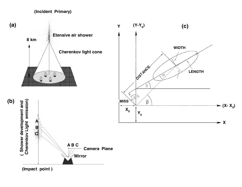
Figure 1: (a) The principle of detecting gamma-rays through the imaging technique (b) Formation of Cherenkov image in the focal plane. (c) Definition of Hillas parameters characterizing each image and used for rejecting the cosmic-ray background. The ellipse represents the approximate outline of the shower image in the focal plane of the telescope.

For each image, which is essentially elliptical in shape, Hillas parameters [6, 50] are calculated to characterize its shape and orientation. The parameters, as depicted in Fig.1c, are obtained using moment analysis and are defined as : LENGTH– The rms spread of light along the major axis of the image (a measure of the vertical development of the shower); WIDTH – The rms spread of light along the minor axis of the image (a measure of the lateral development of the shower); DISTANCE– The distance from the centroid of the image to the centre of the field of view; ($\alpha$)–The angle between the major axis of the image and a line joining the centroid of the image to the position of the source in the focal plane; SIZE – Sum of all the signals recorded in the clean Cherenkov image; FRAC2– The degree of light concentration as determined from the ratio of the two largest PMT signals to sum of all signals ( also referred to as Conc.). In the pioneering work of the Whipple Observatory [4], only one parameter (AZWIDTH) was used in selecting $\gamma$-ray events. Later, the technique was refined to Supercuts / Dynamic Supercuts procedure where cuts based on the WIDTH and LENGTH of the image as well as its orientation are used for segregating the gamma rays from the background cosmic-rays [50]

5.2 Statistical analysis of various parameters for selecting the optimal features

The success of any classification technique depends on the proper selection of the variables which are to be used for the event segregation and the agreement between the expected and the actual distributions of these variables. Fig.2 shows the distributions of the image parameters LENGTH, WIDTH, DISTANCE and $\alpha$ for simulated protons and for the actual Cherenkov events recorded by the telescope.

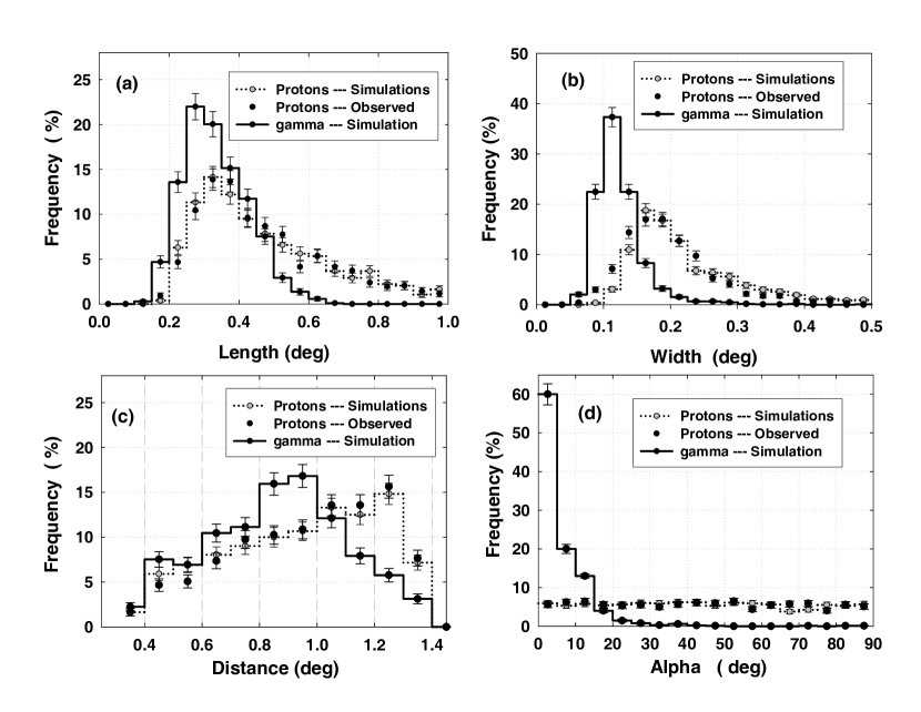
Figure 2: Comparison of image parameter distributions (a) LENGTH, (b) WIDTH, (c) DISTANCE and (d) ($\alpha$) from real and the Monte Carlo simulated data for proton events. The simulated image parameter distribution of $\gamma$-rays has also been shown in the figure for comparison.

The data plotted here has been first subjected to pre-filtering cuts with $SIZE\geq$ 50 photoelectrons (pe) and (0.4${}^{0}\leq DISTANCE\leq 1.4^{0}$) in order to ensure that the events recorded are robust and well contained in the camera. The simulated image parameter distribution of $\gamma$-rays has also been shown in the figure for comparison. The observed image parameter distributions are found to closely match the distributions obtained from simulations for proton-initiated showers, thus suggesting that the response of the telescope is reasonably close to that predicted by simulations. For converting the event SIZE, recorded in charge to digital counts, to corresponding number of photoelectrons, we have used a conversion factor of 1pe $\cong$6.5 counts [42]. In order to understand and improve upon the existing $\gamma$/hadron segregation methods it is important to estimate the discriminating capability of each of the Cherenkov image parameters and their correlations[7]. The image parameters considered for this correlation study are : SIZE, LENGTH, WIDTH, DISTANCE, FRAC2 and $\alpha$.

In order to select image parameters which are best suited for $\gamma$/ hadron separation we have applied the following tests: Student’s t-test, Welch’s t-test, Mann Whitney U-test ( also known as Wilcoxon rank-sum test) and the Kolmogorov - Smirnov test (K S test) [51]. The Student’s t-test and Welch’s t-test belong to the category of parametric tests which assume that the data are sampled from populations that follow a Gaussian distribution. While as, the Students unpaired t- test assumes that the two populations have the same variances, the Welch’s t-test is a modification of the t- test which does not assume equal variances. Tests that do not make any assumptions about the population distribution are referred to as nonparametric tests. Mann Whitney U-test and Kolmogorov - Smirnov test belong to this category of tests. While the nonparametric tests are appealing because they make fewer assumptions about the distribution of the data, they are less powerful than the parametric tests. This means that the corresponding probability values tend to be higher, making it harder to detect real differences as being statistically significant. When large data samples are considered, the difference in power is minor. Furthermore, it is worth mentioning here that the parametric tests are robust to deviations from Gaussian distributions, so long as the samples are large.

In order to apply the above mentioned tests to simulated data of $\gamma$-ray and proton initiated showers we have used $\sim$ 6000 events each, at a zenith angle of 25⁰ and the results of these one-dimensional tests are summarized in Table 1.

Table 1: Statistic values of various parametric and non-parametric statistical tests. Larger value of the statistic indicate that corresponding probability of rejecting the null hypothesis, that the $\gamma$-ray data sample and the proton-data sample come from the same population, is low.

	$Student^{\prime}s$	$Welch^{\prime}s$	$Mann-Whitney$	$KS$
	$t-test$	$t-test$	$U-test$	$D-test$
	$t$	$t$	$z$	$D$
$SIZE$	$1.95$	$1.94$	$8.66$	$0.09$
$LENGTH$	$138.80$	$138.75$	$90.20$	$0.85$
$WIDTH$	$120.96$	$120.28$	$84.75$	$0.76$
$DISTANCE$	$19.65$	$19.64$	$17.18$	$0.18$
$FRAC2$	$200.84$	$200.94$	$92.69$	$0.90$
$ALPHA$	$112.57$	$112.53$	$82.89$	$0.76$

Since the P-values (i.e the probability of rejecting the null hypothesis that the $\gamma$-ray data sample and the proton-data sample come from the same population) are usually very small we have instead used the value of the corresponding statistic for rejecting or accepting the null hypothesis. In other words t-statistic values are given in the Table. 1 for expressing the results of Student’s t-test and Welch’s t-test. Similarly, for Mann Whitney U test the z-statistic values are given in the table (where $z=(U-m_{U})/\sigma_{U}$ with $m_{U}$ and $\sigma_{U}$ as the mean and the standard deviation of U). For the Kolmogorov Smirnov test we have calculated D-statistic (i.e maximum vertical distance between the two cumulative frequency distributions). On examining Table 1 it is evident that four image parameters (viz., LENGTH, WIDTH, FRAC2 and $\alpha$) have a significant potential of providing efficient $\gamma$/ hadron separation. Larger the value of the corresponding statistic, lower is corresponding probability of rejecting the null hypothesis that the $\gamma$-ray data sample and the proton-data sample come from the same population.

In order to estimate the statistical relationship between two image parameters for $\gamma$-ray data sample and the proton-data samples separately we have also calculated the Pearson product-moment correlation coefficient. Following the standard procedure, it is obtained by dividing the covariance of the two variables by the product of their standard deviations. The closer the coefficient is to either -1 or 1, the stronger the correlation between the variables. The results of this study, obtained separately for $\gamma$-ray and proton-data samples, are presented in Tables 2 and 3, respectively.

Table 2: Correlation matrix for simulated $\gamma$-ray data sample at a zenith angle of 25⁰. The values listed below for each correlation coefficient (numbers within parentheses) are the corresponding z-statistic values obtained using Fisher transformation.

Notations used are SIZ=SIZE, LEN=LENGTH, WID=WIDTH, DIS=DISTANCE, FR2=FRAC2. $SIZ$ $LEN$ $WID$ $DIS$ $FR2$ $\alpha$ $SIZ$ $1.000$ $0.394$ $0.474$ $0.072$ $-0.441$ $-0.037$ $(---)$ $(33.206)$ $(41.692)$ $(5.603)$ $(38.051)$ $(2.881)$ $LEN$ $0.394$ $1.000$ $0.615$ $0.038$ $-0.709$ $0.196$ $(33.206)$ $(---)$ $(60.452)$ $(2.908)$ $(78.069)$ $(15.466)$ $WID$ $0.474$ $0.615$ $1.000$ $-0.396$ $-0.569$ $0.456$ $(41.692)$ $(60.452)$ $(---)$ $(33.360)$ $(53.680)$ $(39.649)$ $DIS$ $0.072$ $0.038$ $-0.396$ $1.000$ $-0.034$ $-0.366$ $(5.603)$ $(2.908)$ $(-33.360)$ $(---)$ $(-2.615)$ $(30.491)$ $FR2$ $-0.441$ $-0.709$ $-0.569$ $-0.034$ $1.000$ $-0.064$ $(38.051)$ $(78.069)$ $(53.680)$ $(-2.61)$ $(---)$ $(4.927)$ $\alpha$ $-0.037$ $0.196$ $0.456$ $-0.366$ $-0.064$ $1.000$ $(2.881)$ $(15.466)$ $(39.649)$ $(30.491)$ $(4.927)$ $(---)$

Table 3: Correlation matrix for simulated proton data sample at a zenith angle of 25⁰. The values listed below for each correlation coefficient (numbers within parentheses) are the corresponding z-statistic values (obtained using Fisher transformation).

	$SIZ$	$LEN$	$WID$	$DIS$	$FR2$	$\alpha$
$SIZ$	$1.000$	$0.036$	$0.273$	$-0.301$	$-0.083$	$-0.008$
	$(--)$	$(2.757)$	$(21.950)$	$(2.332)$	$(6.472)$	$(0.624)$
$LEN$	$0.036$	$1.000$	$0.360$	$-0.023$	$-0.618$	$0.086$
	$(2.757)$	$(--)$	$(29.916)$	$(1.792)$	$(60.947)$	$(6.691)$
$WID$	$0.273$	$0.360$	$1.000$	$-0.036$	$-0.510$	$0.005$
	$(21.950)$	$(29.916)$	$(--)$	$(2.806)$	$(46.998)$	$(0.368)$
$DIS$	$-0.301$	$-0.023$	$-0.036$	$1.000$	$-0.006$	$0.012$
	$(2.332)$	$(1.792)$	$(2.806)$	$(--)$	$(0.481)$	$(0.958)$
$FR2$	$-0.083$	$-0.618$	$-0.510$	$-0.006$	$1.000$	$-0.028$
	$(6.472)$	$(60.947)$	$(45.998)$	$(0.481)$	$(--)$	$(2.154)$
$\alpha$	$-0.008$	$0.086$	$0.005$	$0.012$	$-0.028$	$1.000$
	$(0.624)$	$(6.691)$	$(0.368)$	$(0.958)$	$(2.154)$	$(--)$

The values of the t-statistic corresponding to each correlation coefficient are also given in these Tables (numbers within parentheses). These values can be used for assessing the significance of the correlation. Larger value of the z-statistic indicates that the corresponding probability of rejecting the null hypothesis that the observed value comes from a population in which correlation coefficient $\sim$ 0, is low. If the correlation coefficient is $\rho$ the Fisher transformation can be defined as:

$$z=\frac{1}{2}ln\left(\frac{1+\rho}{1-\rho}\right)$$ (1)

The Fisher $\rho$-to-z transformation [52] has also been applied to assess the significance of the difference between two correlation coefficients ( say $\rho_{1}$ and $\rho_{2}$) found in two independent samples. The relevant expression to calculate this is given by :

$$z_{12}=\left(\frac{|\rho_{1}-\rho_{2}|}{\sqrt{\frac{1}{n_{1}-3}+\frac{1}{n_{2}-3}}}\right)$$ (2)

where $\rho_{1}$ and $\rho_{2}$ are the two correlation coefficients, $n_{1}$ and $n_{2}$ are respectively the number of data points used while calculating $\rho_{1}$ and $\rho_{2}$. Table 4 gives the values for the Fisher matrix of various image parameters for the simulated $\gamma$/proton sample.

Table 4: Fisher Matrix for the simulated $\gamma$/hadron data sample at a zenith angle of 25⁰. The matrix can be used to assess the significance of the difference between two correlation coefficients.

	$SIZ$	$LEN$	$WID$	$DIS$	$FR2$	$\alpha$
$SIZ$	$--$	$20.83$	$12.87$	$5.6$	$21.30$	$1.59$
$LEN$	$20.83$	$--$	$18.65$	$3.32$	$8.95$	$6.16$
$WID$	$12.87$	$18.65$	$--$	$20.97$	$4.56$	$26.70$
$DIS$	$5.60$	$3.32$	$20.97$	$--$	$1.51$	$21.68$
$FR2$	$21.30$	$8.95$	$4.56$	$1.51$	$--$	$1.96$
$\alpha$	$1.59$	$6.16$	$26.7$	$21.68$	$1.96$	$--$

On examining Tables 2, 3 and 4, one can select the image parameters for achieving optimum $\gamma$/hadron segregation. This can be done on the basis of identifying parameters for which the difference between their correlation coefficients is maximum. As seen in Table 4, WIDTH-$\alpha$ pair yields the largest Fisher test value. Furthermore, it is also encouraging to find that the other well known characteristics of Cherenkov image parameters are in good agreement with our results. For example, dependence of the image shape parameters (i.e LENGTH and WIDTH) on SIZE for $\gamma$-rays. Both these parameters yield positive correlation coefficient of $\sim$0.394 and $\sim$0.474 as shown in Table 2. Since SIZE parameter of an image provides an approximate estimate of the $\gamma$-ray primary energy both these parameters are expected to be correlated with the event SIZE. The modification of the Supercuts procedure to Dynamic (or extended) Supercuts follows the same principle. Negative correlation between DISTANCE and $\alpha$ for $\gamma$-rays coming from a point source is also seen in Table 2 in accordance with the expected relationship between these image parameters. Thus, on the basis of results presented in Tables 2, 3 and 4, one can confidently say that there is a sufficient scope for utilizing the differences in the correlation between various image parameters for developing alternate $\gamma$/hadron segregation methodologies.

Keeping in view the fact that, for proton initiated showers (as also in general for other cosmic-ray primaries), the image parameter $\alpha$ is expected to be independent of other image parameters because of the isotropic nature of the cosmic-rays we will not use it in the ANN-based $\gamma$/hadron segregation methodology. Justification for following this approach is also evident in Table 3, where for the proton data sample, one finds negligible correlation between $\alpha$ and other image parameters. Thus, for extracting the $\gamma$-ray signal from the cosmic-ray background, we will use the frequency distribution of the $\alpha$ parameter for the ANN selected events. The distribution is expected to be flat for cosmic-rays and should reveal a peak at smaller $\alpha$ values for $\gamma$-rays coming from a point source. In all, we will use the following six image parameters in the ANN-based $\gamma$/hadron segregation methodology : Zenith angle ($\theta$), SIZE, LENGTH, WIDTH, DISTANCE and FRAC2. Use of $\theta$ angle as an additional variable can be justified by keeping in view the fact that as $\theta$ angle increases, the line of sight distance to the shower maximum also increases, making all projected dimensions of the shower (i.e, LENGTH and WIDTH) smaller. The shape parameters LENGTH and WIDTH are expected to approximately scale as $\propto$ $cos(\theta)$.

6 ANN methodology and a brief description of algorithms used

A neural network is a parallel distributed information processing structure consisting of processing elements (which can process a local memory and carry out localized information processing operations) interconnected together with unidirectional signal channels called connections. Each processing element has a single output connection which branches into many collateral connections as desired. All of the processing that goes on within each processing element must be completely local , i.,e it must depend upon only the current values of the input signals arriving at the processing element via impinging connections and upon the values stored in local memory of the processing elements . ANNs like humans, learn by example, and can be configured for a specific problem through a learning process that involves adjustments of the synaptic connections, called weights which exist between neurons. A network is composed of a number of interconnected units, each unit having an input/output characteristics. The output of any unit is determined by its I/O characteristics, its interconnection to other units and external inputs. The feed-forward ANN is the simplest configuration and is constructed using layers where all nodes in a given layer are connected to all nodes in a subsequent layer. The network requires at least two layers, an input layer and an output layer. In addition to this, the network can include any number of hidden layers with any number of hidden nodes in each layer. The signal from the input vector propagates through the network layer by layer till the output layer is reached. The output vector represents the predicted output of the ANN and has a node for each variable that is being predicted.

Depending upon the architecture in which the individual neurons are connected and the error minimization scheme adopted, there can be several possible ANN configurations. While algorithms like Standard backpropagation (along with its varients like the backprop-momentum, Vanilla backprop, Quickprop) and the Resilient backpropation come under the category of Local search algorithms, Conjugate Gradient methods, Levenberg-Marquardt algorithm and One Step Secant belong to the category of Global search algorithm. Hybrid algorithm category constitutes models like Higher Order Neuron and Neuro Fuzzy systems. The Standard Backpropagation network [53], is the most thoroughly investigated ANN algorithm till date. Backpropagation using gradient descent however converges very slowly. The success of this algorithm in solving large-scale problems, although depends critically on user-specified learning rate and momentum parameters, there are however no standard guidelines for choosing these parameters. The Resilient backpropagation(RProp) algorithm was proposed by Reidmiller [54], to expedite the learning of a backpropagation algorithm. Unlike the standard Backpropagation algorithm, RProp uses only partial derivative signs to adjust weight coefficients. In the above backprop based gradient descent algorithms, it is difficult to obtain a unique set of optimal parameters, due to the existence of multiple local minima. The presence of these local minima, hampers the search for global minimum because these algorithms frequently get trapped in local minima regions and hence, incorrectly identify a local minimum as the global minimum.

The conjugate scale gradient algorithms [55] initially use the gradient to compute a search direction and then a line search algorithm is used, to find the optimal step size along a line in the search direction. The Levenberg algorithm involves the use of ”blending method” between the steepest descent method employed by the backpropagation/resilient algorithm and the quadratic rule employed in conjugate algorithms. The original Levenberg algorithm was improved further by Marquardt, resulting in the Lavenberg-Marquardt algorithm [56] by incorporating the information about the local curvature, hence forcing to move further in the direction, in which the gradient is smaller in order to get around the classic ”error valley”. More so, gradient descent based algorithms like backpropagation despite being popular among researchers are not known to be efficient algorithms due to the fact that the gradient vanishes at the solution. Hessian-based algorithms like the Lavenberg-Marquardt, on the contrary, allow the network to learn more subtle features of a complicated mapping. The training process converges as the solution is approached, because the Hessian does not vanish at the solution. The Lavenberg-Marquardt algorithm is basically a Hessian-based algorithm for nonlinear least square optimization [57]. One Step Secant method is an approximation of the Gauss-Newton method for error minimization. The advantage of this method is the smaller memory requirement and lesser computation time, since unlike other algorithms it does not store the complete Hessian matrix, instead at each training iteration it assumes that the previous Hessian was the identity matrix. This has an added advantage that the new search direction can be found without having to compute the matrix inverse [58]. Higher Order Neuron model [59] is the one which includes the quadratic and higher order basis functions in addition to the linear basis functions to reduce the learning complexity.

Neuro-fuzzy systems are models where ANN models are combined with Fuzzy systems to use the best features of both models. While as ANN’s are known to be powerful in reaching a solution, Fuzzy systems have an advantage in comparison to ANN for explaining the decision rules better [60]. Apart from employing these methods we felt that the study would be incomplete without the use of the comparatively lesser used ”backprop - momentum” (backpropagation with momentum term added to the learning rule). The momentum term allows network to respond to local gradient and other trends in the error surface. Without the momentum term network may get stuck in some shallow within the local minima.

It is however important to mention here that for real world problems, the above definitions serve only as a guideline and the actual performance of the ANN models on real world problems does not necessarily follow the above theoretical predictions. Therefore, these varied algorithms under the ANN domain can not be used as off the shelf algorithms until sufficient expertise in the field is obtained. There are several other issues involved in designing and training a multilayer neural network. These are : (a) Selecting appropriate number of hidden layers in the network; (b) Selecting the number of neurons to be used in each hidden layer; (c) Finding a globally optimal solution that avoids local minima; (d) Converging to an optimal solution in a reasonable period of time; (e) Overtraining of the network and (f) Validating the neural network to test for overfitting.

While as, a lot of emphasis has been put lately on the use of Random Forest (RF) technique as an efficient tool for $\gamma$-hadron segregation, we believe that a properly selected and well trained neural net algorithm is equally as efficient for this purpose. The results obtained by [15] in their study obtained a Quality factor (QF) of $\sim$ 2.8 and $\sim$ 3.0 for Random Forest and ANN methods respectively when applied to the MAGIC data. The maximum significance also turns out to be comparable at $\sim$ 8.74$\sigma$ and $\sim$ 8.75$\sigma$ for RF and ANN respectively. In another study conducted by Boinee et al. [61] on the MAGIC Cherenkov telescope experiment, detailed comparison of RF, ANN, Support Vector Machines and Classification Trees have been presented. While as, the optimized RF technique resulted in a classification accuracy of $\sim$ 81.24 $\%$, the classification accuracy for ANN turned out to be $\sim$81.75$\%$ with a mean error rate of $\sim$0.276 and $\sim$ 0.256 for the Random Forest and ANN techniques respectively, thereby suggesting that the two techniques are at best comparable. The results obtained from other methods turn out to be quite inferior compared to the ANN and Random Forest, suggesting that both the methods are equally suitable.

7 Gamma/hadron separation using ANN

7.1 Preparation of Training, testing and validation data

Training the ANN means iteratively minimizing the error between the desired output and the ANN generated value, with respect to the network weights. Clearly, in order for the network to yield appropriate outputs for given inputs, the weights must be set to suitable values. This is done by ’training’ the network on a set of input vectors, for which the ideal outputs (targets) are already known. For training the ANN we have used $\sim$13750 $\gamma$-ray simulated events following a power law distribution with a differential spectral index of $\sim$-2.6. This data-base was obtained by combining together $\sim$2750 events each at 5 different zenith angles ($\theta$ = 5⁰, 15⁰, 25⁰, 35⁰ and 45⁰). The cosmic ray data of $\sim$11290 events, used for training the ANN, is the actual experimental data recorded by the TACTIC telescope and was prepared in the following manner. Around one-third of the data used ($\sim$ 3163 events) were recorded in the Crab Nebula off source direction. From the Crab Nebula on-source data base, collected between Nov.10, 2005 - Jan. 30, 2006, we used another ($\sim$ 3163 events) for which $\alpha\geq 27^{\circ}$ and are hence certainly cosmic-ray events. The remaining one-third portion of the data was taken from $\sim$30h of Mrk 421 off-source observations and this data was collected during the same observing season. The zenith angle of the off-source observation was restricted to $\leq 45^{\circ}$. The reason for generating the training data in this manner was to ensure that all possible systematic influences on the training of the network such as variable sky brightness in different directions are also included during the training procedure. Using the experimental data-base for the protons is a useful way of training, since it helps ANN to recognize the latent patterns, if any, in a better way which can otherwise be difficult to replicate in simulations e.g, in situations when the sky brightness is higher than what has been assumed in simulations. The importance of using real background hadronic events instead of simulated events has also been demonstrated in [14].

The test data set consists of an independently generated sample of about 44831 events (mixture of $\sim$ 24603 simulated $\gamma$-ray and $\sim$ 20228 actual cosmic-ray events), which has not been used while training the ANN. This data set has exactly the same format as the training data set and is generated in the same manner as the training data. A validation data sample of $\sim$ 29798 events ( mixture of 16424 simulated $\gamma$-ray and 13374 actual cosmic-ray events) is used for verifying that the network retains its ability to generalize and is not ”over-trained”.

7.2 ANN training and optimizing the number of hidden layer nodes

The network used in this work comprises 6 nodes in the input layer with one each node for Zenith angle ($\theta$), SIZE, LENGTH, WIDTH, DISTANCE and FRAC2 and one neuron in the output layer whose value decides to which class the output is to be categorized. This value is designated as 0.1 or 0.9 depending upon whether the event in question is a gamma-ray or a cosmic-ray event respectively. In order to determine the optimum number of neurons in the hidden layer we evaluate the Mean Square Error (MSE) generated by the network. The MSE for the network is defined as:

$$MSE=\frac{1}{2}{\frac{1}{PI}\sum\limits_{p=1}^{P}\sum\limits_{i=1}^{I}\left(\frac{D_{pi}-O_{pi}}{D_{pi}}\right)^{2}}$$ (3)

where $D_{pi}$ and $O_{pi}$ are the desired and the observed values and P is the number of training patterns and I is the number of outputs, which happens to be 1 in our case. Thus MSE defined above, is the sum of the squared differences between the desired output and the actual output of the output neurons averaged over all the training exemplars [62]. The ANN algorithms used in the present work are the following: Backpropagation, Resilient Backpropagation, Backprop-momentum, Conjugate Gradient, One step secant, Higher Order Neurons, Levenberg Marquardt and the Neuro fuzzy.

With regard to choosing the number of nodes in the hidden layer, it is well known that, while using too few nodes will starve the network of the resources that it needs to solve a particular problem; choosing too many nodes has the risk of potential overfitting where the network tends to remember the training cases instead of generalizing the patterns. In order to find the optimum number of nodes in the hidden layer we employed a two step procedure. In the first step we varied the number of nodes in the hidden layer from 5 to 60 (in steps of 5 up to 40 and in steps of 10 thereafter) and noted down the MSE for each of the configurations. In the second step, we deliberately used significantly higher number of nodes in the hidden layer (equal to 90) and then applied the Singular Value Decomposition (SVD) method for identifying the redundant nodes [32, 63-65]. It is worth mentioning here that determining the optimum number of neurons in the hidden layer by sequentially increasing the number of nodes from 60 onwards involves massive computational effort, hence the need of applying the SVD method is justified.

In the SVD method, the weight matrix (denoted by F in the present work) was generated by finding the output of each of the 90 nodes before subjecting them to the nonlinear transformation (i.e output of the hidden node). With a total of 25040 training patterns and one hidden layer with 90 nodes, the matrix F has thus 25040 rows and 90 columns. The SVD of the matrix F is given by F=U S V ^T, where U and V are the orthogonal matrices and S is a diagonal matrix with 25040 rows and 90 columns. The matrix S contains the singular values of F on its diagonal. The dominance of the significant singular values of F ( say g out of a total p singular values) is found out by using the so called percentage of energy explained ($P_{ex}$) and is defined as :

$$P_{ex}=\frac{\sum_{i=1}^{g}{S_{i}}^{2}}{\sum_{i=1}^{p}{S_{i}}^{2}}\times 100$$ (4)

where $S_{1},S_{2},S_{3}-----S_{p}$ are the singular values of F arranged in their descending order [66]. The results of this study are shown in Fig 3. where $P_{ex}$ is plotted as a function of number of nodes in the hidden layer for a representative example of 4 ANN algorithms. Consolidated results concerning the performance of the various algorithms with regard to their corresponding MSE values for the training, test and validation data samples are given in Table 5.

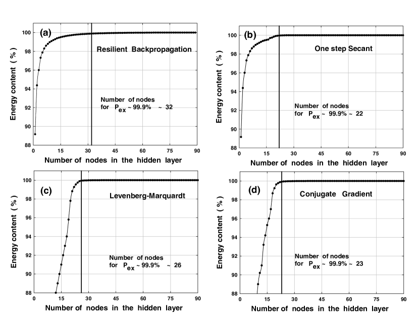
Figure 3: Percentage of energy explained ($P_{ex}$) as a function of number of nodes in the hidden layer for some representative algorithms : (a) Resilient backpropation (b) One Step Secant (c) Levenberg-Marquardt algorithm and (d) Conjugate Gradient. The optimum number of nodes for $P_{ex}$ $\sim$ 99.9 $\%$ is also marked in the figures by full vertical lines.

The results presented in this table shown separately for 35 and 90 nodes in the hidden layer, can be used for checking whether the ANN algorithm is ”over-trained” or not. When the network is over-trained, the MSE for the test and validation data samples are expected to be significantly higher than the corresponding value of MSE achieved during training.

Table 5: MSE values of various ANN algorithms for the training, test and validation data samples. The two values presented in the table correspond to 35 and 90 nodes in the hidden layer.

$Algorithm$	$Train\ 35/90$	$Test\ 35/90$	$Valid\ 35/90$
$Backpropagation$	$0.103/0.102$	$0.103/0.103$	$0.103/0.103$
$BackpropMomentum$	$0.156/0.158$	$0.157/0.159$	$0.156/0.158$
$ResilientBackprop$	$0.035/0.033$	$0.036/0.035$	$0.036/0.034$
$ScaleConjugate$	$0.047/0.040$	$0.046/0.041$	$0.047/0.041$
$OneStepSecant$	$0.053/0.050$	$0.053/0.051$	$0.053/0.051$
$LavenbergMarquardt$	$0.017/0.015$	$0.017/0.030$	$0.017/0.031$
$HigherOrder$	$0.039/0.033$	$0.040/0.033$	$0.040/0.034$
$NeuroFuzzy$	$0.062/0.062$	$0.062/0.063$	$0.062/0.062$

The optimum number of nodes for $P_{ex}$ $\sim$ 99.9 $\%$ is also marked in the figures by full vertical lines. For $P_{ex}$ $\sim$ 99.9 $\%$, one can easily find from the this figure that the optimum number of nodes needed for obtaining the desired results varies between $\sim$22 to $\sim$ 32. Except for the Backpropagation-Momentum algorithm which requires only $\sim$5 nodes, the remaining algorithms are also found to yield optimum performance with $\sim$20 to $\sim$30 nodes in the hidden layer. The reason for Backprop momentum requiring too few nodes can be understood from the manner in which the algorithm is trained. In this algorithm, momentum term is added to the Backprop to enhance the training time with a slight compromise on the performance of the network. This effect is seen in our case also where we see the Backprop Momentum algorithm yielding the worst MSE value compared to all other algorithms.

On examining Fig.3 and Table 5 one can arrive at the following conclusions : (i) None of the ANN algorithms used in this work are under trained or over trained if about 35 nodes are used in the hidden layer. (ii) Increasing the number of nodes beyond 35 results in only a marginal reduction in the MSE. (iii) The MSE value yielded by the Levenberg-Marquardt method with 35 nodes is found out to be the lowest compared to all other ANN algorithms. (iv) Increasing the number of nodes from 35 to 90 leads to the problem of overfitting in the Levenberg-Marquardt method. (v) For the remaining algorithms no overfitting problem is seen when 90 nodes are used in the hidden layer. The overfitting of the Levenberg-Marquardt (with 90 nodes in the hidden layer) is most probably related to the way in which the training is performed in this algorithm, more specifically how the algorithm accounts for error as well as the gradient information based on blending between the gradient descent method and the Gauss Newton rule. The Levenberg-Marquardt trains in such a way that large steps are taken in the direction of low curvature to skip past the plateaus quickly, and smaller steps are taken in the direction of high curvature to slowly converge to the global minima. Thus every narrow valley or plateau, even if as a result of noise in the data, is important for this method. Hence, when larger number of nodes are presented ( i.e, 637 weights for the 90 nodes versus 252 weights for the 35 nodes in the hidden layer), the algorithm becomes sensitive even to the noise values present in the data, which with lesser number of nodes could have been ignored. The source of noise in our training/test data-base is as result of inherent fluctuations in the shower development process. On the basis of the above argument one can thus safely use 35 nodes in the hidden layer for all the algorithms.

It is worth mentioning here that the modification of the ANN structure by analyzing how much each node contributes to the actual output of the neural network and dropping the nodes which do not significantly affect the output is also referred to as pruning. The basic principle of pruning relies on the fact that if two hidden nodes give the same outputs for every input vector, then the performance of the neural network will not be affected by removing one of the nodes in the hidden layer. In the SVD approach, redundant hidden nodes cause singularities in the weight matrix which can be identified through inspection of its singular values. A non-zero number of small singular values indicates redundancy in the initial choice for the number of hidden layer nodes and the approach can be safely used for eliminating these nodes to attain the pruned network model.

A plot of the mean square error as a function of the number of nodes in the hidden layer for the most popular standard backpropagation network and the Lavenberg-Marquardt algorithm with Sigmoid transfer function is shown in Fig.4a.

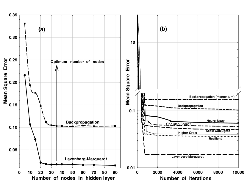
Figure 4: (a) Mean square error as a function of number of nodes in the hidden layer for the Backpropagation and the Lavenberg-Marquardt algorithms. (b) Mean square error for various ANN algorithms as a function of number of iterations with 35 nodes in the hidden layer.

While the MSE at the end of the training, for 35 nodes in the hidden layer, is $\sim$0.1032 for the backpropagation network, the corresponding vaule for the Lavenberg-Marguardt algorithm is found to be $\sim$0.0171. Although the MSE yielded by the Lavenberg-Marguardt algorithm is found to be lower than the MSE values of other training algorithms, including the backpropagation algorithm, the reason for showing the MSE for the backpropagation algorithm is mainly because it has been considered as a ”work-horse” in the field of neural computation.

The variation of the MSE as a function of number of iterations for all ANN algorithms used, is shown in Fig.4b. The number of neurons in the hidden layer was thus fixed at 35 nodes for all these algorithms. In all above algorithms, the training is continued till the MSE error reaches a plateau and does not decrease any further. About 10,000 iterations were generally found to be sufficient to train the ANN on various algorithms. This superior convergence of Lavenberg-Marquardt algorithm over the conventionally used backpropagation algorithm and/or resilient backprop is not totally unexpected and has been demonstrated by us on standard benchmark and regression problems [60].

It is worth mentioning here that for studying the performance of the various ANN algorithms we have used BIKAS (BARC-IIT Kanpur ANN Simulator) ANN package [67] and MATLAB [68,69] neural net packages. While as, MATLAB has been used for backpropagation, resilient backpropagation, Scale Conjugate, backprop-momentum, Lavenberg-Marquardt, and One Step Secant algorithms, the BIKAS package has been used for Higher Order Network and Neuro-Fuzzy models.

7.3 Testing and validation of Lavenberg-Marquardt ANN algorithm

Since MSE error returned by the Lavenberg-Marquardt algorithm is lower than the MSE error values of other methods including the backpropagation method, we have used only this algorithm on the test data set for a more descriptive analysis. When the test data-base is presented to the network, instead of yielding the desired output as 0.1 or 0.9, the ANN outputs a range of values between 0.1 to 0.9. The broad distributions around 0.1 and 0.9, returned after testing the prior trained ANN algorithm, instead of the desired 0.1 or 0.9, is on account of the inherent shower to shower fluctuations on an event to event basis even though train and test data is generated in a similar manner. The response of the network (i.e., frequency distribution of the selected events) for the test data sample comprising simulated $\gamma$-rays and actual background as a function of the ANN output is shown in Fig.5a.

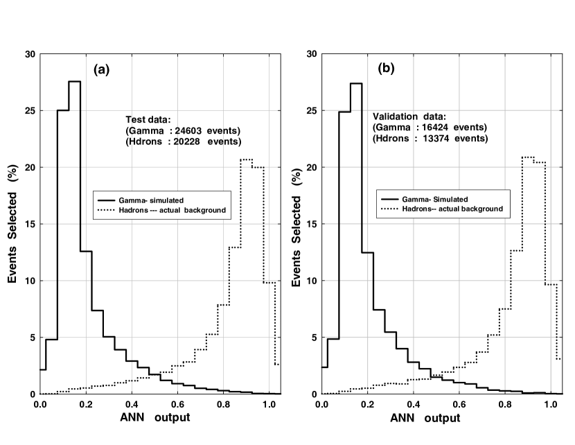
Figure 5: (a) ANN output of Lavenberg-Marquardt algorithm in response to simulated $\gamma$-rays and actual background events of the test data sample comprising a total 44831 events. (b) Same as (a) except for an independant validation data sample comprising a total 29798 events. No cut on $\alpha$ has been applied to the data presented in these figures.

The results obtained for the validation data sample are shown in Fig. 5b. Excellent matching of the results obtained for the test and validation data clearly demonstrates that ANN has indeed ”learned” and simply not remembered the classification. It is important to mention here that no cut on $\alpha$ has been applied to the data presented in these figures.

8 Determination of optimum ANN cut value

For determining the ANN output cutoff value ($\eta_{cut}$), which will optimize the separation of the two event classes (i.e $\gamma$-ray and cosmic-rays), one can maximize either Quality Factor ($QF$) or more adequately, statistical significance ($N_{\sigma}$). Following their standard definitions [15], these are given by :

$$QF=\frac{N_{\gamma}/N_{\gamma 0}}{\sqrt{N_{p}/N_{p0}}}=\frac{f_{\gamma}}{\sqrt{f_{p}}}\\$$ (5)

$$N_{\sigma}=\frac{N_{\gamma}}{\sqrt{N_{\gamma}+2N_{p}}}$$ (6)

where $N_{\gamma}$ and $N_{p}$ are the number of $\gamma$-rays and hadrons, respectively, after classification; $N_{\gamma 0}$ and $N_{p0}$ are the number of $\gamma$-rays and hadrons, respectively, before classifier and $f_{\gamma}$ and $f_{p}$ are the corresponding acceptances for $\gamma$-rays and hadrons. Although many groups have used QF for optimizing the performance of their classification methods [14] , we have optimized the performance of the ANN on the basis of maximizing $N_{\sigma}$. The reason for this is the fact that a high value of $QF$ can also result from tight cut which can reduce the $\gamma$-ray retention capability of the classification method. Furthermore, maximization of $N_{\sigma}$ also ensures that classification procedure in not biased unfavorably towards higher energies. Optimization on the basis of maximizing $N_{\sigma}$ has also been followed by other groups [13,15].

It is worth mentioning here that definition of statistical significance ($N_{\sigma}$) given above can be only used when $N_{\gamma}$ is known beforehand which is possible only when one is dealing with simulated data. Since, in case of actual data collected with Cherenkov imaging telescopes, $N_{\gamma}$ can also be calculated statistically by subtracting the expected number of background events ( e.g $27^{\circ}\leq\alpha\leq 81^{\circ}$ used by us in [39] and in this work) from the $\gamma$-ray domain events (e.g $\alpha\leq 18^{\circ}$ in our case) the definition of statistical significance given above needs to be modified. While we have used the above expression of $N_{\sigma}$ for estimating $\eta_{cut}$, the significance of the $\gamma$-ray events found in the actual Crab Nebula data has been calculated by following a more rigorous method of using maximum likelihood ratio of Li and Ma [70].

The value of $\eta_{cut}$ defines the decision boundary between the two event species and in order to determine its optimum value we used a data sample of about 12953 events (mixture of 8865 simulated $\gamma$-ray and 4088 actual cosmic-ray events). The zenith angle range of these events was again chosen to be in the range (0-45)^∘. Since the value of $N_{\sigma}$ depends critically on the number of $\gamma$-rays present in the data we have considered only $N_{\gamma 0}$$\sim$177 ( i.e $\sim$2$\%$ of the total $\gamma$-rays present in the data sample) for determining the optimum value of $\eta_{cut}$. The event is classified as a $\gamma$-ray like event only if the corresponding ANN output ($\eta$) is $\leq$ $\eta_{cut}$ and $\alpha\leq 18^{\circ}$. The calculation was performed by varying $\eta_{cut}$ from 0.05 to 1.0 in steps of 0.05 and recording $N_{\sigma}$ at each value of $\eta_{cut}$. The results of this study are given in Fig.6 which shows variation of $N_{\sigma}$ as a function of $\eta_{cut}$ for the Levenberg-Marquardt based ANN algorithm.

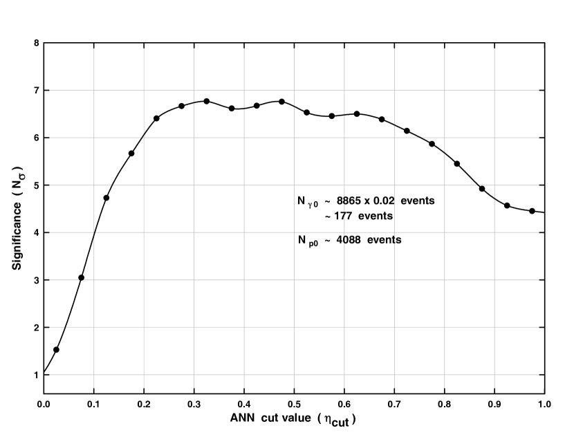
Figure 6: Variation of statistical significance ($N_{\sigma}$) as a function of ANN cut value ( $\eta_{cut}$) for the Levenberg-Marquardt algorithm.

On examining this figure one can see that maximum value of $N_{\sigma}$ $\sim$ 6.8$\sigma$ is obtained at $\eta_{cut}$ $\sim$0.475. The above data has also been used for evaluating the performance of other ANN algorithms and finding their optimum $\eta_{cut}$ values. The results of this study are summarized in Table 6 where, in addition to $N_{\sigma}$ values yielded by different algorithms, we also give the corresponding $\eta_{cut}$ range within which $N_{\sigma}$ stays constant. The lower value of $\eta_{cut}$ defines the tight cut and higher value designates the loose cut.

Table 6: Maximum value of the statistical significance $N_{\sigma}$ yielded by various ANN algorithms along with corresponding $\eta_{cut}$ range with in which $N_{\sigma}$ stays constant. The lower value of $\eta_{cut}$ defines the tight cut and higher value defines the loose cut.

$Algorithm$	$\eta_{cut}$	$N_{\sigma}$
$Backpropagation$	$0.40-0.67$	$5.21$
$Backpropagation\ monemtum$	$0.30-0.57$	$5.33$
$Resilient\ Backprop$	$0.42-0.67$	$5.25$
$Scale\ Conjugate$	$0.40-0.67$	$4.80$
$One\ Step\ Secant$	$0.42-0.67$	$5.25$
$Lavenberg\ Marquardt$	$0.30-0.62$	$6.80$
$Higher\ Order$	$0.40-0.70$	$4.80$
$Neuro\ Fuzzy$	$0.40-0.67$	$4.47$
$Dynamic\ Super\ cut$	$---$	$6.09$

The value of $N_{\sigma}$ achieved with Dynamic Supercuts is also shown in the table for comparison. It is quite evident from the table that out of 8 different ANN algorithms studied here, Levenberg-Marquardt algorithm yields the best results. The value of $N_{\sigma}$ for other algorithms is found to vary from $\sim$ 4.5$\sigma$ ( Higher order network) to $\sim$ 5.3$\sigma$ (backprop-momentum). Because of the superior performance of the Levenberg-Marquardt algorithm, we will only use this algorithm for analyzing the actual Crab Nebula data.

Referring back to Fig.6, since the change in $N_{\sigma}$ is insignificant when $\eta_{cut}$ is varied from $\sim$0.3 to $\sim$0.5, we will use a value of $\eta_{cut}$ $\sim$0.5 for analyzing the actual Crab Nebula data. Admittedly, using $\eta_{cut}$ $\sim$0.5 also increases the cosmic ray background. The reason for choosing the higher $\eta_{cut}$ value is to ensure that we retain maximum number of $\gamma$-rays from the source. For sources which are weaker than the Crab Nebula one can use $\eta_{cut}$ $\sim$0.3 so that contamination from more background can be reduced. Since our main preference is to observe relatively stronger sources such as blazars using $\eta_{cut}$ $\sim$0.5 is an obvious choice if we want to measure their energy spectra beyond energies of $\sim$10TeV. Following this approach of choosing the tight cuts for detecting weaker/new sources and loose cuts for obtaining the energy spectrum, is a well known procedure which is adopted by almost all the groups who work on Cherenkov imaging telescopes.

9 Application of the ANN methodology to the Crab Nebula data collected with the TACTIC telescope

In order to study the $\gamma$/hadron segregation potential of the ANN methodology, we have applied this selection method to the Crab Nebula data collected with the TACTIC telescope. For this purpose we reanalyzed the Crab Nebula data for $\sim$101.44 h collected during Nov. 10, 2005 - Jan. 30, 2006. The zenith angle during the observations was $\leq$45^∘ and the data was collected with inner 225 pixels ($\sim$ 4.5^∘ $\times$ 4.5^∘) of the full imaging camera with the innermost 121 pixels ($\sim$ 3.4^∘ $\times$ 3.4^∘) participating in the trigger. The standard two-level image ’cleaning’ procedure with picture and boundary thresholds of 6.5$\sigma$ and 3.0$\sigma$, respectively was employed to obtain the clean Cherenkov images. Details of this analysis procedure and the data collecting methodology for this period can be found in [42]. The purpose of this image cleaning procedure is to take care of the fluctuations in the image which arise due to electronic noise and night sky background variations. These clean Cherenkov images were then characterized by calculating their standard image parameters like LENGTH, WIDTH, DISTANCE, $\alpha$, SIZE and FRAC2. Before investigating the $\gamma$/hadron segregation potential using ANN methodology, we will first apply the standard Dynamic Supercuts procedure [8] to the data for extracting the $\gamma$-ray signal from the background cosmic-ray events.

The cut values used for the analysis are the following : $0.11^{\circ}\leq LENGTH\leq(0.260+0.0265\times\ln S)^{\circ}$, $0.06^{\circ}\leq WIDTH\leq(0.110+0.0120\times\ln S)^{\circ}$, $0.52^{\circ}\leq DISTANCE\leq 1.27^{\circ}cos^{0.88}\theta$, $SIZE\geq 450d.c$ ( where 6.5 digital counts$\equiv$1.0 pe ), $\alpha\leq 18^{\circ}$ and $FRAC2\geq 0.35$. It is important to emphasize here that the Dynamic Supercuts $\gamma$-ray selection criteria used in the present analysis are the same which we had used in our previous work [39] for developing an ANN-based energy reconstruction procedure for the TACTIC telescope. Since the present work uses the same data-base as well as the same energy reconstruction procedure, we will consider the previous work [39] as some sort of benchmark for the present study. Admittedly, there may be a scope for optimizing the previously used Dynamic Supercuts further (e.g by using cuts which depend on both energy and zenith angle), but the results of this study will be presented elsewhere.

A well established procedure to extract the $\gamma$-ray signal from the cosmic-ray background using a single imaging telescope is to plot the frequency distribution of $\alpha$ parameter which is expected to be flat for the isotropic background of cosmic events [8]. For $\gamma$-rays, coming from a point source, the distribution is expected to show a peak at smaller $\alpha$ values. Defining $\alpha\leq 18^{\circ}$ as the $\gamma$-ray domain and $27^{\circ}\leq\alpha\leq 81^{\circ}$ as the background region, the number of $\gamma$-ray events is then calculated by subtracting the expected number of background events (calculated on the basis of background region) from the $\gamma$-ray domain events. The number of $\gamma$-ray events obtained after applying the above cuts are found to be $\sim$(928$\pm$100) with a statistical significance of $\sim$9.40$\sigma$. The significance of the excess events has been calculated by using the maximum likelihood ratio method of Li $\&$ Ma [70]. The $\alpha$-distribution is given in Fig. 7a and the corresponding differential energy spectrum of the Crab Nebula shown in Fig. 7b, has been computed using the following formula:

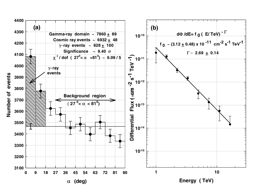
Figure 7: (a) Crab Nebula $\alpha$-plot for $\sim$101.44 h of data using Dynamic Supercuts $\gamma$-ray selection criteria. (b) The corresponding differential energy spectrum of the Crab Nebula as measured by the TACTIC telescope.

$$\frac{d\Phi}{dE}(E_{i})=\frac{\Delta N_{i}}{\Delta E_{i}\sum\limits_{j=1}^{5}A_{i,j}\eta_{i,j}T_{j}}$$ (7)

where $\Delta N_{i}$ and $d\Phi(E_{i})/dE$ are the number of events and the differential flux at energy $E_{i}$, measured in the ith energy bin $\Delta E_{i}$ and over the zenith angle range of 0^∘-45^∘, respectively. $T_{j}$ is the observation time in the jth zenith angle bin with corresponding energy-dependent effective area ($A_{i,j}$) and $\gamma$-ray acceptance ($\eta_{i,j}$). The 5 zenith angle bins (j=1-5) used are 0^∘-10^∘, 10^∘-20^∘, 20^∘-30^∘, 30^∘-40^∘ and 40^∘-50^∘ with effective collection area and $\gamma$-ray acceptance values available at 5^∘, 15^∘, 25^∘, 35^∘ and 45^∘. The number of $\gamma$-ray events ($\Delta N_{i}$) in a particular energy bin is calculated by subtracting the expected number of background events, from the $\gamma$-ray domain events. The $\gamma$-ray differential spectrum, shown in Fig. 7b, has been obtained after using appropriate values of effective collection area and $\gamma$-ray acceptance efficiency (along with their energy and zenith angle dependence). A power law fit $(d\Phi/dE=f_{0}E^{-\Gamma})$ with $f_{0}\sim(3.12\pm 0.48)\times 10^{-11}cm^{-2}s^{-1}TeV^{-1}$ and $\Gamma\sim 2.69\pm 0.14$ is also shown in Fig 7b. The fit has a $\chi^{2}/dof\sim 3.64/6$ with a corresponding probability of $\sim$0.72. Details of the energy reconstruction procedure can be seen in [39] which uses 3:30:1 ANN configuration with SIZE, DISTANCE and Zenith angle as the inputs to the neural net.

While applying the already trained Lavenberg-Marquardt based ANN network, with 6:35:1 configuration, for extracting the $\gamma$-ray signal from the data, the number of $\gamma$-ray events are found out to be $\sim$(1141$\pm$106) with a statistical significance of $\sim$11.07$\sigma$. A value of $\eta_{cut}$ $\sim$0.50 has been used for selecting $\gamma$-ray events and only those events are allowed to go for classification with ANN, which satisfy the prefiltering cuts (SIZE $\geq$ 50pe and $0.4^{\circ}$ $\leq$ DISTANCE $\leq$ $1.35^{\circ}$). The $\alpha$-distribution of the ANN selected events is given in Fig.8a, while as the corresponding differential energy spectrum is shown in Fig.8b.

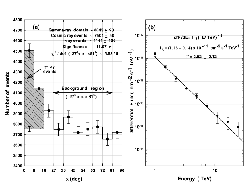
Figure 8: (a) Crab Nebula $\alpha$-plot for $\sim$101.44 h of data using Lavenberg-Marquardt based ANN network $\gamma$-ray selection criteria. (b) The corresponding differential energy spectrum of the Crab Nebula when ANN network is used for selecting $\gamma$-ray like events.

A power law fit $(d\Phi/dE=f_{0}E^{-\Gamma})$ with $f_{0}\sim(1.16\pm 0.14)\times 10^{-11}cm^{-2}s^{-1}TeV^{-1}$ and $\gamma\sim 2.52\pm 0.12$ is also shown in Fig 8b. The fit has a $\chi^{2}/dof\sim 4.58/7$ with a corresponding probability of $\sim$0.71. Reasonably good matching of the Crab Nebula spectrum with that obtained by the Whipple and HEGRA groups [71,72] reassures that the procedure followed by us for selecting $\gamma$-ray like events as well as obtaining the energy spectrum of a source, is quite reliable.

On comparing the results of Dynamic Supercuts $\gamma$-ray selection procedure (Fig.7) with the Lavenberg-Marquardt based ANN network (Fig.8) it is evident that the performance of the later is somewhat superior, both with regard to improving the statistical significance of the $\gamma$-ray signal as well as in selecting more number of $\gamma$-rays. Although the improvement (i.e gain of $\sim$213 gamma-ray like events along with signal enhancement from 9.4$\sigma$ to 11.07$\sigma$) looks to be only modest, the main advantage accruing from the ANN methodology is that it is more efficient at higher energies which has allowed us to extend the Crab Nebula energy spectrum up to an energy of $\sim$24TeV. At $\gamma$-ray energies above $\sim$9 TeV, the Lavenberg-Marquardt based ANN network selects $\sim$(85$\pm$28) events as against $\sim$(24$\pm$9) events selected by the Dynamic Supercuts procedure.

When a value of $\eta_{cut}$ $\sim$0.30 is used, the number of $\gamma$-ray events are found out to be $\sim$(680$\pm$67) with a statistical significance of $\sim$10.49$\sigma$ and this is in perfect agreement with the discussion presented in Section 8. Although the use of tight cut (i.e $\eta_{cut}$ $\sim$0.3) yields almost same statistical significance (ignoring slight degradation) as compared to $\eta_{cut}$ $\sim$0.5 cut case, the number of $\gamma$-rays retained are significantly less and it is just for this reason that we preferred to use a somewhat loose cut $\eta_{cut}$ $\sim$0.5.

The performance of the Lavenberg-Marquardt based ANN network was further validated by applying it $\sim$ 201.72 hours of on-source data collected on Mrk 421 with the TACTIC telescope during Dec. 07, 2005 to Apr. 30, 2006. The total data used here also includes observations from Dec. 27, 2005 to Feb. 07, 2006 when the source was found to be in a high state by the TACTIC telescope as compared to the rest of the observation period [42]. When already trained ANN is used for extracting the $\gamma$-ray signal from the data, the number of $\gamma$-ray events are found out to be $\sim$(1493$\pm$121) with a statistical significance of $\sim$12.60$\sigma$. On comparing these results with that obtained by using Dynamic Supercuts [42] which yields, $\sim$(1236$\pm$110) $\gamma$-ray events with a statistical significance of $\sim$11.49$\sigma$, it is reassuring to find that the ANN method is indeed more efficient than the Dynamic Supercuts method. Furthermore, as expected, no signature of a $\gamma$-ray signal is seen when the ANN method is applied to $\sim$ 29.65 hours of off-source data. The results obtained with the ANN method ( $\sim$ 60$\pm$42 with a statistical significance of $\sim$1.46$\sigma$) compare well with the results reported by us earlier using Dynamic Supercuts [42]( $\sim$ 28$\pm$20 with a statistical significance of $\sim$0.71$\sigma$). Detailed results of the reanalysis using the ANN including the energy spectrum Mrk-421 will be presented elsewhere.

Successful detection of $\gamma$-rays from Mrk-421 thus clearly demonstrates the capability of the properly trained ANN to extract a $\gamma$-ray from a source other than the Crab Nebula. It also indicates that the generalization capability of the ANN can be enhanced if it is trained with the experimental data collected from different directions having somewhat variable sky brightness.

10 Comparison of Dynamic Supercuts and ANN analysis methods

A detailed study for comparing the performance of Dynamic Supercuts and ANN analysis methods has also been conducted by us so that the overall $\gamma$-retention capability of the Dynamic Supercuts and ANN analysis methods can be compared. One of the ways to study this is to use the Monte Carlo simulated data for $\gamma$-rays and plot the dependence of effective collection areas as a function of primary energy for the two $\gamma$-ray selection methodologies. The results of this study are shown in Fig.9 where effective collection areas for the two $\gamma$-ray selection methodologies is plotted as a function of energy for two representative zenith angle values of 15^∘ and 35^∘.

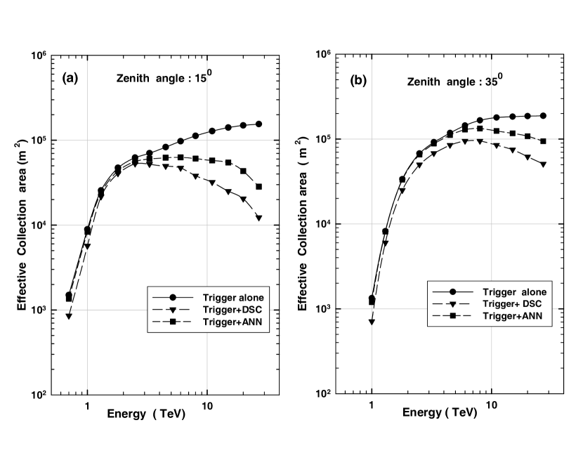
Figure 9: Effective collection area as a function of the primary $\gamma$-ray energy for simulated $\gamma$-ray at showers zenith angles of (a) 15^∘ and (b)35^∘. While top most curve (labeled as Trigger alone) gives the effective area when no cuts are applied to the data, the remaining 2 curves (labeled as Trigger+ DSC and Trigger+ANN) represent when Dynamic Supercuts and ANN analysis methods, respectively are applied to the data

.

Apart from showing the effective areas ( i.e $A_{\gamma}(E)f_{\gamma}(E)$) for the two $\gamma$-ray selection methodologies, the corresponding effective area when no cuts are applied to the data ( i.e $A_{\gamma}(E)$) is also shown for comparison. The results displayed in the figure clearly indicate that the efficiency of Dynamic Supercuts is biased towards lower energies ( particularly at lower zenith angles). On the other hand, it is the superior performance of Lavenberg-Marquardt based ANN network ( i.e more collection area at higher energies) which has enabled us to retain relatively higher number of events at energies above $\sim$9 TeV in the actual data as compared to the Dynamic Supercuts procedure.

The above conclusion has been further validated by obtaining scatter plots of various image parameters and the results of this study are shown in Fig.10. This figure displays scatter plots of LENGTH, WIDTH, DISTANCE and FRAC2 as a function SIZE for $\sim$8358 events which have been characterized as $\gamma$-ray like by the ANN algorithm and have $\alpha\leq 18^{\circ}$.

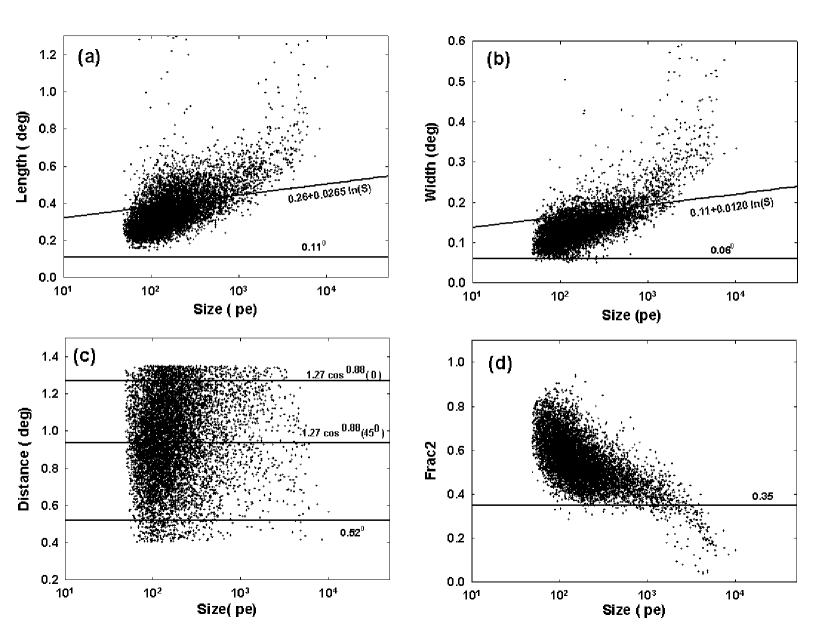
Figure 10: Scatter plots of (a) LENGTH (b) WIDTH (c) DISTANCE and (d) FRAC2 as a function of SIZE which have been characterized as $\gamma$-ray like by the ANN and have $\alpha\leq 18^{\circ}$. The Dynamic Supercuts boundaries are also shown in the figure as full lines.

For comparison, the Dynamic Supercuts boundaries are also shown in the figure as full lines. It is quite evident from the figure that the ANN method in not just selecting the same population of events as the Dynamic Supercuts but the ANN is also sensitive to selecting events which lie outside the strict Dynamic Supercuts boundaries. An alternative way to assess the residual population of events selected by ANN is to perform a logical NOT selection between the ANN and the Dynamic Supercuts methods. On performing this selection the number of $\gamma$-ray events are found out to be $\sim$(453$\pm$74) with a statistical significance of $\sim$6.27$\sigma$ which again suggests that the ANN method is more useful than the Dynamic Supercuts methods while determining the energy spectrum of $\gamma$-ray source. On performing a logical AND selection between the ANN and the Dynamic Supercuts methods the number of $\gamma$-ray events yielded are $\sim$(655$\pm$71) corresponding to a statistical significance of $\sim$9.50$\sigma$.

In order to understand the performance of ANN for $\gamma$-rays at higher energies (i.e, the events which eventually contribute to the last 3 energy bins of Fig.8) Fig.11 displays the scatter plot of $\sim$606 events which have been characterized as $\gamma$-ray like by the ANN and which have their $\alpha\leq 18^{\circ}$.

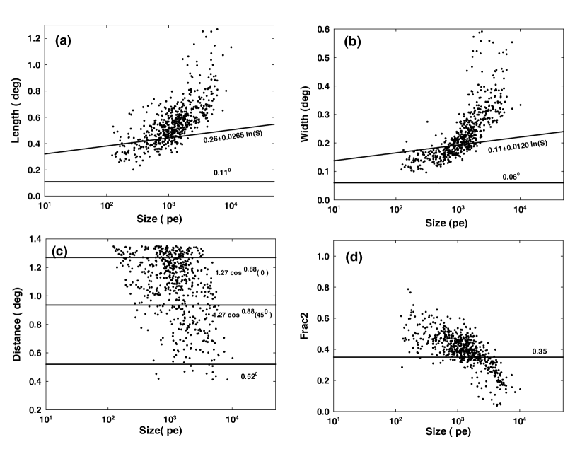
Figure 11: Scatter plots of (a) LENGTH (b) WIDTH (c) DISTANCE and (d) FRAC2 as a function of SIZE which have been characterized as $\gamma$-ray like by the ANN. Apart from having $\alpha\leq 18^{\circ}$ these events also have energy above $\sim$9 TeV. The Dynamic Supercuts boundaries are also shown in the figure as full lines.

In other words the data presented in this figure represents a subsample of the data used in Fig.10 with an additional condition that the $\gamma$-ray like events should have energies above $\sim$9 TeV. The capability of the ANN in selecting events which lie outside the strict Dynamic Supercuts boundaries is again evident from the figure. For example, presence of relatively large number of event outside the LENGTH cut boundary (Fig.11a) clearly demonstrates that the efficiency of Dynamic Supercuts in retaining $\gamma$-rays is biased towards lower energies. It is important to point here that there are background cosmic-ray events also present in Fig.10 and Fig.11 which are classified as $\gamma$-ray like events by the event selection methodology. Since subtraction of the background events (estimated from $27^{\circ}\leq\alpha\leq 81^{\circ}$ region), from the $\gamma$-ray domain (defined as $\alpha\leq 18^{\circ}$), will cancel out these events (in statistical sense) and it does not matter how the energy estimate for background event was obtained.

Since differences in the observed energy spectrum of several active galactic nuclei, especially at higher energies, can be used to study absorption effects at the source or in the intergalactic medium due to interaction of $\gamma$-rays with the extragalactic background photons [73, 74], unarguably, efficient retention of high energy $\gamma$-ray events is always preferable. Superior performance of the ANN at higher energies can thus play an important role in the understanding the absorption effects at the source or in the intergalactic medium.

It is worth mentioning here that once satisfactory training of the ANN is achieved, the corresponding ANN generated weight-file can be easily used by an appropriate subroutine of the main data analysis program for selecting $\gamma$-ray like events. Use of a dedicated ANN software package is thus necessary only during the training of the ANN and is not needed there after. Also, compared to the conventional $\gamma$/hadron separation methods, the ANN-based procedure also offers advantages like applicability over a wider zenith angle range and implementation ease.

11 Conclusions

Atmospheric Cherenkov imaging telescopes, especially Monoscopic systems, have to cope up with a deluge of cosmic-ray background events and the capability to suppress these against the genuine $\gamma$-rays is one of the main challenges which limits the sensitivity of these telescopes. The main purpose of this paper is to study the $\gamma$ / hadron segregation potential of various ANN algorithms for the TACTIC telescope, by applying them to the Monte Carlo simulated and the observation data on the Crab Nebula. The results of our study indicate that the performance of Levenberg-Marquardt based ANN algorithm is somewhat superior to the Dynamic Supercuts procedure especially beyond $\gamma$-ray energies of $\geq$ 9 TeV. Since for real world problems it is not an easy task to identify the most suitable ANN algorithm by just having a look at the problem, our results suggest that while investigating the comparative performance of other ANN algorithm, the Levenberg-Marquardt algorithm deserves a serious consideration. The main advantage of using the ANN methodology for $\gamma$/ hadron segregation work is that it is more efficient in retaining higher energy $\gamma$-ray events and this has allowed us to extend the TACTIC observed energy spectrum of the Crab Nebula up to an energy of $\sim$24TeV. Reasonably good matching of the Crab Nebula spectrum as measured by the TACTIC telescope with that obtained by the other groups reassures that the ANN-based $\gamma$/hadron segregation method and also the procedure for obtaining the energy spectrum of a $\gamma$-ray source are quite reliable.

12 Acknowledgements

The authors would like to convey their gratitude to all the concerned colleagues of the Astrophysical Sciences Division for their contributions towards the instrumentation, observation and analysis aspects of the TACTIC telescope. The authors would also like to thank the anonymous referees for their valuable comments which have helped us to improve the quality of the paper.

References

- [1] J. Holder 2012 [astro-ph.HE/1204.1267v1]
- [2] F. Aharonian et al., Rep. Prog. Phys., 71 (2008) 096901.
- [3] P.M. Chadwick et al., J.Phys. G : Nucl. Part. Phys., 35 (2008) 033201.
- [4] T.C. Weekes et al., Astrophys. J, 342 (1989) 379
- [5] A. Daum et al., Astropart. Phys., 8 (1997) 1.
- [6] A.M. Hillas, Proc. 19th ICRC , La Jolla, 3 (1985) 445.
- [7] F.A.Aharonian et al., Nucl. Instr. and Meth. A, 302 (1991) 522.
- [8] G.Mohanty et al., Astropart. Phys., 9 (1998) 15.
- [9] P.T.Reynolds et al., J.Phys. G : Nucl. Part. Phys., 19 (1993) 1217.
- [10] S.Danaher et al., Astropart. Phys., 1 (1993) 357.
- [11] A. Haungs et al., Astropart. Phys 12 (1999) 145
- [12] A.K.Razdan et al., Astropart. Phys 17 (2002) 497
- [13] A.Chilingarian, Pattern Recognition Letters 16 (1995) 33
- [14] P.T.Reynolds and D.J.Fegan, Astropart. Phys., 3 (1995)137.
- [15] R.K. Bock et al., Nucl. Instrum. Meth. A516 (2004) 511.
- [16] J.Albert et al., Nucl. Instrum. Meth. A 588 (2008) 424
- [17] M.de.Naurois and L. Rolland, Astropart. Phys., 32 (2009) 231
- [18] F. Dubois et al., Astropart. Phys., 32 (2009)73
- [19] S. Ohm et al., Astropart. Phys., 31 (2009)383
- [20] H.Krawczynski et al., Astropart. Phys., 25 (2006)380.
- [21] K.Hornik et al., Neural Networks , 2, (1989) 359.
- [22] H.Gish, Proc. IEEE Int. Conf. Acoustic Speech Signal Processing, (1990) 1361
- [23] M.D.Richard and L Lippmann, Neural Computation, 3 (1991) 461
- [24] L. Lonnblad et al., Phys. Rev. Lett. 65 (1990) 1321.
- [25] C. Bortolotto et al., Nucl. Instr. and Meth. A. 306( 1991) 459
- [26] P. Abreu et al., Phys. Lett. B 295 (1992) 383
- [27] B. Brandl et al., Nucl. Instr. and Meth. A. 324( 1993) 307
- [28] R. Tagliaferri et al., Neural Networks 16 (2003) 297
- [29] R.A.Vaze et al., Phy. Rev. D., 45(1992)356.
- [30] M.J.Lang, J.Phys. G : Nucl. Part. Phys., 24 (1998) 2279 .
- [31] B.M.Schafer et al., Nucl. Instrum. Meth. A 465 (2001) 394.
- [32] V.K. Dhar et al., Meas. Sci. Technol. 21 (2010) 015112
- [33] V.K. Dhar et al., Experimental Astronomy 10 (2000) 487
- [34] S.Bussino and S.M.Mari, Astropart. Phys., 15 (2001) 65
- [35] G. M Maneva et al., Nucl. Instrum. Meth. A 502 (2003) 789.
- [36] D.Dumora et al., Nucl. Phys. B ( Proc. Suppl.), 97 (2001) 255.
- [37] De-Mitri et al., Nucl. Instr. and Meth. A. 525( 2004) 132
- [38] S. Westerhoff et al., Astropart. Phys 4 (1995) 119.
- [39] V.K. Dhar et al., Nucl. Instr. and Meth. A, 606 (2009) 795
- [40] K.K. Yadav et al., Nucl. Instr. and Meth. A, 527( 2004) 411.
- [41] R. Koul et al., Nucl. Instr. and Meth. A, 578 (2007) 548.
- [42] K.K. Yadav et al., Astropart. Phys., 27 (2007) 447.
- [43] S.V. Godambe et al., J.Phys. G : Nucl. Part. Phys., 34 (2007) 1683.
- [44] S.V. Godambe et al., J.Phys. G : Nucl. Part. Phys., 35 (2008) 065202.
- [45] K.K. Yadav et al., J.Phys. G : Nucl. Part. Phys., 36 (2009) 085201.
- [46] P.Chandra et al., J.Phys. G : Nucl. Part. Phys., 37 (2010) 125201.
- [47] P.Chandra et al., J.Phys. G : Nucl. Part. Phys., 39 (2012) 045201.
- [48] D. Heck et al., Report FZKA 6019 Forshungszentrum, Karlshrue, (1998).
- [49] M.K. Koul et al., Nucl. Instr. and Meth. A, 646 (2011) 204.
- [50] P.T.Reynolds et al., Astrophys. J. 404(1993) 206.
- [51] R.J.Barlow Guide to use of statistical methods in Physical Sciences, John Wiley and sons 1987
- [52] W.H. Press et al., Numerical Recipies in C, Cambridge University Press India 2007.
- [53] D.E. Rumelhart et al., Nature 323 (1986) 533
- [54] M. Reidmiller, Computer Standards Interfaces, 16 (1994) 265.
- [55] M. F. Moller et al., Neural Networks 6, (1993) 525.
- [56] D. W. Marquardt J Soc. Indust. Appl. Math. 11 (1963) 431
- [57] M.T. Hagan et al., IEEE Trans. Neural Networks, 5 (1994) 6
- [58] R. Battiti, Neural Computation, 4 (1992) 141
- [59] C.L. Giles et al Appl. Opt 26 (1987) 4972
- [60] C.T.Lin et al., Neural-Fuzzy Systems (Prentice Hall, USA, 1996)
- [61] P. Boinee et al., Trans. on Engg. Computing and Tech. 7 (2005) ISSN 1305-5313
- [62] J.M.Zurada, Introduction to Artificial Neural Sustems, Jaico Publishing House, Mumbai, 2006.
- [63] P.P.Kanjilal et al., Electronic Letters 29 (1993) 17.
- [64] D.C.Psichogios et al., IEEE Trans. Neural Networks 5 (1994) 513.
- [65] E.J.Teoh, et al., IEEE Trans. Neural Networks 17 (2006) 1623.
- [66] S. Chakroborty et al., Speech Communications 52 (2010) 693.
- [67] V.K.Dhar et al., Pramana, Jour. of Physics 74, (2010) 307
- [68] http://www.mathworks.in
- [69] S.N.Sivananda Introduction to Neural Networks using MATLAB, McGraw-Hill Companies 2011
- [70] T.P.Li and Y.Q. Ma , Astrophys. J, 272 (1983) 317.
- [71] A.M. Hillas et al., Astrophys. J, 503 (1998) 744
- [72] F.A Aharonian et al., Astrophys. J, 614 (2004) 897
- [73] F.A. Aharonian et al., Nature. 440 (2006) 1018.
- [74] J. Albert et al., Science. 320 (2008) 1752.