Mesoscopic fluctuations of conductance of a helical edge contaminated by magnetic impurities

Abstract

Elastic backscattering of electrons moving along the helical edge is prohibited by time-reversal symmetry (TRS). We demonstrate, however, that an ensemble of magnetic impurities may cause TRS-preserving quasi-elastic backscattering, resulting in interference effects in the conductance. The characteristic energy transferred in a backscattering event is suppressed due to the RKKY interaction of localized spins (the suppression is exponential in the total number of magnetic impurities). We predict the statistics of conductance fluctuations to differ from those in the conventional case of a one-dimensional system with quenched disorder.

The constitutive porperty of a two-dimensional topological insulator is the presence of helical edge states at its bounaries. The electron states propagating in opposite directions along an edge form Kramers doublets and are protected against elastic backsacattering by the time-reversal symmetry (TRS). The fundamental consequence is the universality of the zero-temperature conductance of a topological insulator. Experimental demonstration of such universality is viewed as the confirmation of the existence of topological insulators. The existing experiments clearly distinguish the topological insulators from highly-resistive “conventional” ones molenk2007 . However, the measured conductance approaches the universal value only in very short (less than $1\mu$m long) samples. Conductance of longer samples typically is lower, indicating the presence of electron backscattering.

Mechanisms of the backsacttering are a matter of ongoing debate. Current proposals utilize the Coulomb interaction between the electrons of helical edge kane-mele ; moore ; schmidt or scattering of an electron off a localized magnetic impurity macejko1 ; macejko2 ; tanaka . In all theoretical models considered so far the electron backscattering is either deeply inelastic or, as in the case of a magnetic impurity at temperatures exceeding the Kondo scale, quasi-elastic and incoherent due to the flips of the impurity spin macejko1 ; tanaka . In either case the bacskcattering, while suppressing the value of conductance $G$ at finite temperatures does not lead to mesoscopic fluctuations in $G$, in contrast with the low-temperature electron transport in conventional low-dimensional conductors.

In this work we show that interference effects in the conductance of a helical edge contaminated by an ensemble of magnetic impurities are actually possible. Unlike a single impurity, spins in an ensemble are coupled by a long-range RKKY interaction. The latter prevents individual spins from flipping in the course of electron backscattering. That allows for a coherent superposition of the electron de Broglie waves reflected by different impurities. Remarkably, this picture does not contradict TRS: the electron reflection remains inelastic. However, it is associated with a collective flip of a block of spins. Therefore its amplitude is sensitive to the spatial structure of the electron wave. Large number of spins in the block also ensures a parametrically small (exponential in the number of spins) energy transfer in the scattering event. This energy sets a mild lower limit for the temperature at which the considered quantum-coherent phenomenon can be observed.

Interference in electron reflection manifests itself in mesoscopic fluctuations of conductance $G,$ seen, for example when the chemical potential of electrons is continuously changed by a gate voltage $V_{g}$. In conventional one-dimensional wires such fluctuations are due to the varying interference conditions for the potential scattering of electrons. At sufficiently low temperatures such conductance fluctuations are pronouncedly non-Gaussian. In the regime of weak backscattering they obey the Rayleigh statistics. In contrast, we find that the variations of $G$ with $V_{g}$ caused by an ensemble of magnetic impurities tend to be close to gaussian except for temperature close to the spin-glass crossover.

We consider a topological insulator with a simple helical edge molenk2007 ; kane-mele such that the spin $\mathbf{s}$ of an electron occupying an edge state has a conserved component $s_{z}$ in some fixed direction $\hat{z}.$ A magnetic impurity in a vicinity of the edge will experience two important interactions: a local single-ion anisotropy induced by the bulk spin-orbit coupling and a local exchange coupling to the electrons of the edge. (The direct exchange between the impurity spins is negligible at low impurity density.) We assume the anisotropy to be of easy-axis type with some anisotropy constant $K>0.$ The exchange coupling of the edge-state electrons to the impurity spin will generally be anisotropic and depend on the position of the impurity. The effective low-energy Hamiltonian describing the helical edge with $N$ magnetic impurities is

$${\cal H} ={\cal H}_{0}-\sum_{i=1}^{N}K\left({\mathbf{n}}\cdot{\mathbf{S}^{i}}\right)^{\!2}+\hbar v\sum_{i=1}^{N}\kappa_{ab}^{i}S^{i}_{a}\tau_{b}(x_{i})\,,$$ (1)

$${\cal H}_{0} =\hbar v\int dx\psi^{\dagger}(x)(-i\tau_{z}\nabla)\psi(x)\,.$$ (2)

Here the two-component spinor fields $\psi(x)$ represent the smooth (on the scale provided by the Fermi wave length $2\pi/k_{F}$) envelope of the electron operators, $\boldsymbol{\tau}(x)=\psi^{\dagger}(x)e^{-ik_{F}\tau_{z}x}\boldsymbol{\tau}e^{ik_{F}\tau_{z}x}\psi(x)$ is the electron spin density operator where $\boldsymbol{\tau}$ is the spin vector composed of the three Pauli matrices; $v$ is the electron velocity, $\mathbf{S}^{i}$ is the $i$’th impurity spin. We will see that the interference effects in $G$ appear if the spin anisotropy axis $\mathbf{n}$ is different from $\hat{z}$ and the impurities have spin $S>1.$ We assume the magnetic impurities to be distributed randomly along the sample length $L$ and at random distances from the edge, resulting in random positions $x_{i}$ and coupling constants $\kappa_{ab}^{i}.$ In general, the exchange tensors $\kappa_{ab}^{i}$ and the tensor of single-ion anisotropy should be considered as running coupling constants, depending on the choice of the bandwidth cutoff. The renormalization of the anisotropy is not infrared-divergent. Therefore, assuming that the bare constants $\kappa_{ab}^{i}$ are small, one adds an ultraviolet correction to Eq. (1) of the form

$$\mathcal{H}_{A}=\sum_{i=1}^{N}\delta K_{ab}^{i}S^{i}_{a}S^{i}_{b}$$ (3)

with $|\delta K^{i}|\sim|\kappa^{i}|^{2}\Delta,$ where $\Delta$ is the bandwidth cutoff scale set by the insulator band gap. Renormalization of the tensors $\hat{\kappa}^{i}$ is infrared-divergent, but remains small at energies exceeding the Kondo scale $T_{K}$. The latter is exponentially small in $1/|\kappa^{i}|$ or even a higher power of that parameter, due to the effect of single-ion anisotropy. We note that the itinerant electrons facilitate the RKKY interaction between the impurities, which is of the order of $\hbar v|\kappa^{1}||\kappa^{2}|/x$ for two impurities at distance $x$ from each other. We may ignore the renormalization of $\kappa$ as long as the RKKY exchange is larger than $T_{K}.$

We start the analysis of the model with considering two impurities at distance $x$ from each other. Treating the exchange tensors $\hat{\kappa}^{i}$ as perturbation theory parameters we find the leading-order RKKY interaction

$$\mathcal{H}_{\rm RKKY}=-\frac{\hbar v}{4\pi|x|}S^{1}_{a}\kappa_{ab}^{1}\omega_{bc}(x){P_{cd}}\kappa_{de}^{2}S^{2}_{e}\,.$$ (4)

Here $\omega_{bc}(x)$ is the orthogonal matrix of counterclockwise rotation through angle $2k_{F}x$ about the $z$ axis and ${P_{cd}}=\delta_{cd}-\delta_{cz}\delta_{dz}$ is the matrix of orthogonal projection onto the $xy$ plane. Assuming that $\mathcal{H}_{\rm RKKY},$ Eq. (4), and $\mathcal{H}_{A},$ Eq. (3), are small as compared to the easy-axis anisotropy $K$, we may apply secular perturbation theory to determine the low-energy spectrum of the two-spin system. In the zeroth-order perturbation theory the ground state of the two-spin system is four-fold degenerate with the corresponding eigenspace spanned by four vectors, $|\pm S\rangle_{1}\otimes|\pm S\rangle_{2}$, where $|s\rangle_{i}$ denotes an eigenstate of ${\mathbf{S}}^{i}\cdot{\mathbf{n}}$ with an eigenvalue $s\in\{-S,-S+1,\dots,S-1,S\}$ and the subscript $i=1,2$ labels the Hilbert space attached to the $i$th spin. The secular matrix of perturbation Eq. (4) is conveniently written in terms of operators $\hat{s}_{i}$ acting on the $i$-th spin only:

$$\hat{s}_{i}=|S\rangle^{\phantom{i}}_{i}\langle S|^{\phantom{i}}_{i}-|-S\rangle^{\phantom{i}}_{i}\langle-S|^{\phantom{i}}_{i}\,.$$ (5)

In this notation, the secular matrix takes form of Ising Hamiltonian,

$${\cal H}_{I}=-\delta E\cos(2k_{F}x)\hat{s}_{1}\hat{s}_{2}\,;$$ (6)

here $\delta E=(\hbar v/4\pi|x|)n_{a}\kappa_{ab}^{1}{P_{bc}}\kappa_{cd}^{2}n_{d}.$ Depending on the sign of $\cos(2k_{F}x)$ the ground state of the Hamiltonian (16) is one of the two doublets, $|S\rangle_{1}\otimes|S\rangle_{2}$, $|-S\rangle_{1}\otimes|-S\rangle_{2}$ or $|S\rangle_{1}\otimes|-S\rangle_{2}$, $|-S\rangle_{1}\otimes|S\rangle_{2}$. The ground-state doublet is separated by energy $\sim|\delta E|$ from the excited level, which is also a doublet. Note that for all $S>1$ the contribution of the perturbation Eq. (3) to the secular matrix is purely diagonal and has no effect on the splitting of the ground level.

In higher-order perturbation theory further splitting of the two doubly degenerate energy levels occurs. The dominant effect here is due to the perturbation (3). Indeed, it has non-vanishing matrix elements for transitions in which the projection of one impurity spin is increased (or decreased) by $1$ or $2,$ for example $(\langle S-2|\!\otimes\!\langle S|)\mathcal{H}_{A}(|S\rangle\!\otimes\!|S\rangle)\neq 0.$ For $S>1$ any such transition takes a vacuum state to a virtual state having the energy of the order $K.$ At least $[S-1/2]$ such consecutive transitions (here the symbol $[\dots]$ stands for the integer part of $S$) are needed in order to flip one impurity spin from $-S$ to $S,$ that is to bring the system from a vacuum state to a state in the excited doublet with energy $|\delta E|.$ Taking such processes into account amounts to introducing an off-diagonal correction to the Hamiltonian (6)

$$\Delta\mathcal{H}=\delta K\left(\frac{\delta K}{K}\right)^{[S-1/2]}\sum_{i=1,2}r_{i}|S\rangle_{i}\langle-S|_{i}\,,$$ (7)

where $r_{i}$ are some complex constants of the order of unity. If $|x|\ll(\hbar v/\Delta)\times(K/\delta K)^{[S-1/2]}$, then each doublet in the spectrum of the Ising Hamiltonian (6) will split with the energy of the splitting

$$\varepsilon\sim\delta K\left(\frac{\delta K}{K}\right)^{2[S-1/2]}\frac{\delta K}{|\delta E|}$$ (8)

small compared to $|\delta E|$.

Consider now the combined dynamics of electrons and spins at energies $E\ll{\rm min}(\hbar v/x,K)$. It is described by the Hamiltonian ${\cal H}_{\rm eff}={\mathcal{H}}_{0}+{\mathcal{H}}_{I}+\Delta{\mathcal{H}}+{\mathcal{U}}$ with

$$\mathcal{U}=\hbar v\sum_{i=1,2}\hat{s}_{i}\psi^{\dagger}(x_{i})(\boldsymbol{\xi}_{i}\cdot\boldsymbol{\tau})\psi(x_{i})\,,$$ (9)

where $\boldsymbol{\xi}_{i}=[P\omega(x_{i})\kappa^{i}]\mathbf{n}$. We retain only the $x$ and $y$ components of $\boldsymbol{\xi}_{i}$ which cause electron backscattering,

$$\boldsymbol{\xi}_{i}=\xi_{i}\cdot(\cos 2k_{F}x_{i},\sin 2k_{F}x_{i},0)\,.$$ (10)

At temperatures $T\gg\varepsilon$ we may neglect the term $\Delta{\cal H}$ in ${\cal H}_{\rm eff}$. In that approximation, variables ${\hat{s}_{i}}$ are constants of motion. For each configuration of ${\hat{s}}_{i}$ we evaluate the backscattering current within the Born approximation in ${\cal U}$. The total backscattering current is the Gibbs average of such contributions. It leads to the correction to the ballistic conductance,

$$\delta G=-\frac{e^{2}}{h}\left[\xi_{1}^{2}+\xi_{2}^{2}+2(\boldsymbol{\xi}_{1}\cdot\boldsymbol{\xi}_{2})\eta\right]\,.$$ (11)

The term $2(\boldsymbol{\xi}_{1}\cdot\boldsymbol{\xi}_{2})\eta$ here comes from the interference between the electron waves reflected by the two local magnetic moments. The factor $(\boldsymbol{\xi}_{1}\cdot\boldsymbol{\xi}_{2})$ experiences the conventional Fabry-Pérot oscillations as a function of the Fermi momentum $k_{F}$ with the period $2\pi/|x|$. The factor $\eta=\tanh[\delta E\cos(2k_{F}x)/T]$ also oscillates with the same period; at low temperatures, $T\ll\delta E$, it rapidly changes between $-1$ and $1$ each time $\cos 2k_{F}x$ changes sign.

At the lowest energy scale, $T\lesssim\varepsilon$, one has to account for $\Delta{\cal H}$. It lifts the degeneracy of the ground state and therefore prevents an electron with energy less than $\varepsilon$ from elastic backscattering within the helical edge. In order to investigate the electron conduction in this low-energy regime, we evaluate the backscattered current in a steady non-equilibrium state induced by the source-drain voltage. The application of the Fermi Golden Rule yields

$$I_{\rm BS}=\frac{ve}{8\pi}\int_{-\infty}^{\infty}dp\left[\xi_{1}^{2}+\xi_{2}^{2}+2\eta(\boldsymbol{\xi}_{1}\cdot\boldsymbol{\xi}_{2})\cos(2px)\right]\\ \times\bigg{\{}f_{++}(p)+f_{+-}(p)-f_{-+}(p)-f_{--}(p)\\ +\big{[}f_{++}(p)f_{-+}(p)-f_{+-}(p)f_{--}(p)\big{]}\tanh\frac{\varepsilon}{2T}\bigg{\}}$$ (12)

where

$$f_{\alpha\beta}(p)=\tanh\left(\frac{\hbar vp}{T}+\alpha\frac{eV+\beta\varepsilon}{2T}\right),\quad\alpha,\beta=\pm.$$ (13)

In the linear regime ($V\to 0$) Eq. (12) predicts a correction to the ideal conductance

$$\delta G=-(\xi_{1}^{2}+\xi_{2}^{2})F\left({\textstyle\frac{\varepsilon}{T},0}\right)-2\eta(\boldsymbol{\xi}_{1}\cdot\boldsymbol{\xi}_{2})F\left({\textstyle\frac{\varepsilon}{T},\frac{Tx}{\hbar v}}\right)$$ (14)

with

$$F(w,z)=\frac{e^{2}}{h}\int_{-\infty}^{\infty}d\lambda\frac{2\cosh^{2}(\lambda)\cos\left({2z\lambda}\right)}{\left[\cosh\left(w\right)+\cosh(2\lambda)\right]^{2}}\,.$$ (15)

The second argument of $F(w,z)$ is small in the entire region $T\ll\delta E/\kappa^{2}$, so we may set $z=0$. The $w\gg 1$ asymptote $F(w,0)\sim e^{-w}$ implies that the backscattering correction is exponentially suppressed at $T\ll\epsilon.$ In the opposite limit $w\to 0$ the function $F(w,0)\to 1$ in agreement with Eq. (11) obtained in the $\Delta{\cal H}=0$ approximation. Hereinafter we assume $T\gg\varepsilon$. footnote

Next, we generalize the above considerations to a system of $N>2$ magnetic impurities statistically uniformly distributed with average density $n=N/L$ along the edge of length $L$. The corresponding effective Hamiltonian which allows one considering scattering of electrons with energies $E\lesssim\hbar vn$ has the form ${\cal H}_{\rm eff}={\mathcal{H}}_{0}+{\mathcal{H}}_{\rm Ising}+\Delta{\mathcal{H}}+{\mathcal{U}}$, where $\Delta{\mathcal{H}}$ and ${\mathcal{U}}$ are defined by Eqs. (7) and (9) (with extension of the summation to $N$), and

$$\mathcal{H}_{\rm Ising}=-\frac{\hbar v}{4\pi}\sum_{i<j}\frac{\xi_{i}\xi_{j}\cos 2k_{F}(x_{i}-x_{j})}{|x_{i}-x_{j}|}\hat{s}_{i}\hat{s}_{j}\,,$$ (16)

with $\xi_{i}$ defined in Eq. (10).

The conductance correction evaluated in the Born approximation is

$$\delta G=-\frac{e^{2}}{h}\sum_{i,j}\xi_{i}\xi_{j}\cos 2k_{F}(x_{i}-x_{j})\langle\hat{s}_{i}\hat{s}_{j}\rangle\,.$$ (17)

Here the spin correlation function is

$$\langle\hat{s}_{i}\hat{s}_{j}\rangle=\frac{{\rm Tr}\exp\left(-{\cal H}_{\rm Ising}/T\right)\hat{s}_{i}\hat{s}_{j}}{{\rm Tr}\exp\left(-{\cal H}_{\rm Ising}/T\right)}\,.$$ (18)

In a given sample and at given temperature the conductance correction $\delta G,$ Eq. (17), depends on the Fermi momentum $k_{F}$ through the oscillatory factors in Eq. (17) and in ${\cal H}_{\rm Ising}$, see Eq. (16). In experiment, this dependence take form of random fluctuations of the conductance as the Fermi energy of electrons at the edge is changed. The statistical properties of such fluctuations are fully encoded in the cumulants

$$G_{m}=\lim_{\lambda\to 0}\frac{d^{m}}{d\lambda^{m}}\ln\overline{\exp(\lambda\cdot\delta G)}$$ (19)

where the overline represents the statistical average. We now demonstrate that the statistical properties of conductance fluctuations at the magnetically contaminated helical edge are drastically different from those in the case of the conventional quenched disorder in a one-dimensional conductor.

First, we recall the structure of conductance fluctuations caused by an ensemble of weak quenched scatterers in a usual one-dimensional conductor. At temperatures such that the coherence length and the thermal length $\hbar v/T$ are both greater than the sample length the conductance is temperature-independent. The electron reflection amplitude is, in the Born approximation, a linear superposition of $N$ random complex numbers, $e^{ik_{F}x_{i}},$ where $x_{i}$ is the position of the $i$th impurity. Consequently, in the large $N$ limit the conductance correction obeys the Rayleigh distribution, which is essentially non-Gaussian. In particular, for the second and third cumulants one has $G_{3}=-2G_{2}^{3/2}.$

In contrast, the fluctuations of conductance of the helical edge, Eq. (17), exhibit strong temperature dependence in the whole range of validity of the model (16). We note that the model possesses an intrinsic temperature scale

$$T_{\rm SG}=\frac{\hbar v\xi^{2}n}{4\pi}$$ (20)

defining a crossover from the high-temperature regime, where spins thermally disordered to the “spin glass” regime where spins develop long-range correlations across the sample. For $T\gg T_{\rm SG}$ the model can be investigated by means of the virial expansion.

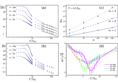
Figure 1: MC data for the statistics of the mesoscopic conductance fluctuations at different temperatures and system sizes. In panel (a) shown is the average conductance $g_{1}$ as a function of temperature. The asymptotes given by Eq. (23) are shown for comparison as solid black lines. Panels (b) shows the second cumulant $g_{2}$ of the conductance distribution. Panel (c) shows the dependence of the first three cumulants at $T=0.5\,T_{\rm SG}$ on the system size. The log-log plot shows a good fit with the $g_{m}\sim N^{m+1}$ scaling. Panel (d) shows the skewness of the distribution of conductance values as a function of temperature.

We assume that the coupling constants $\xi_{i}$ have a Gaussian distribution with the average $\xi$ and introduce the normalized cumulants $g_{m}$ such that

$$G_{m}=\left(\frac{\xi^{2}e^{2}}{h}\right)^{m}\left[g_{m}(\tau,N)-\delta_{m,1}N\right].$$ (21)

The normalized cumulants are functions of the dimensionless temperature $\tau=T/T_{\rm SG}$ and the number of impurities $N=nL.$ At $T\gg T_{\rm SG}$ the spin-spin correlation function in Eq. (17) is given by

$$\langle\hat{s}_{i}\hat{s}_{j}\rangle=\tanh\left(\frac{\hbar v\xi_{i}\xi_{j}\cos 2k_{F}(x_{i}-x_{j})}{4\pi|x_{i}-x_{j}|T}\right).$$ (22)

Substituting Eq. (22) in Eq. (17) and averaging over the uniform distribution of magnetic impurities we find

$$g_{1}(\tau,N)=-\frac{N}{8\pi\tau}\ln\left(\tau N\right)\,.$$ (23)

The logarithm in Eq. (23) is due to the $1/|x_{i}-x_{j}|$ dependence in the large-distance expansion of Eq. (22). The upper cutoff for this dependence is provided by the system size, $N/n,$ while the lower cutoff is defined by the distance $x$ at which the exchange energy $\hbar v\xi^{2}/x$ equals the temperature. For the higher cumulants the virial expansion yields

$$g_{m}(\tau,N)=C_{m}\frac{N}{\tau},\qquad m>1.$$ (24)

Here $C_{m}$ are constants, in particular $C_{2}=0.20304$ and $C_{3}=0.01242.$ Note, that unlike the quenched case the third cumulant is positive. At $NT_{\rm SG}\gg T\gg T_{\rm SG}$ the higher cumulants satisfy $g_{m}^{2}\ll g_{2}^{m}$ therefore the distribution of conductance fluctuations is close to Gaussian.

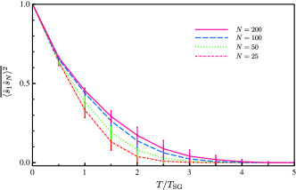
Figure 2: Spin-spin correlation function at the opposite ends of the sample as a function of temperature for various systems sizes. Note that larger system sizes result in stronger correlations at given temperature. This effect is caused by the long-rangedness of the RKKY exchange resulting in the logarithmic renormalization of the spin-spin interaction constant with increasing system size.

With decreasing temperature virial corrections to the spin-spin correlation function (18) become increasingly important. To explore this effect we calculate the first two terms in the virial expansion of the correlator

$$\overline{\langle\hat{s}_{i}\hat{s}_{j}\rangle^{2}}=\frac{1}{2\tau^{2}n^{2}|x_{i}-x_{j}|^{2}}\left(1+\frac{2}{\tau}\ln\tau n|x_{i}-x_{j}|+\dots\right)\,,$$

where $\dots$ stand for the higher-order terms in $1/\tau.$ One can see that no matter how large the temperature $\tau$ is, the virial expansion breaks down at sufficiently large distances. For a given system size $L$ one can define the crossover temperature $\tau_{*}$ such that $1=\tau_{*}^{-1}\ln(nL\tau_{*}).$ Below this temperature equations (23) and (24) are not valid. The crossover temperature $\tau_{*}$ is a monotonically increasing function of the system size. In large systems there exists a parametric window $1<\tau<\tau_{*}$ where the long-range spin-glass correlations are absent, yet the virial expansion is invalid.

In order to investigate $g_{m}(\tau,N)$ at $\tau<\tau_{*}$ we performed Monte Carlo simulations for $N=25,50,100$ and $200.$ For each $N$ we consider $10$ random realizations of quenched impurity positions, assuming $\xi$ to be the same for all impurities. We observe a considerable slowdown of the convergence of Metropolis algorithm for $T<5\,T_{\rm SG}$ caused by the onset of spin glass correlations. To overcome this difficulty we employ parallel tempering, which works efficiently down to $T=0.5\,T_{\rm SG}.$ Numerical results for $g_{1,2}(\tau,N)$ are presented in Fig. 1. In the temperature window $5\lesssim\tau\lesssim 10$ the cumulants experience a sharp increase with decreasing temperature from $g_{m}\sim N$ (see Eq. (24)) to $g_{m}\sim N^{m+1}$ (see Fig. 1 (c) ). For $\tau\lesssim 5$ one can observe the onset of correlations between moments located near the opposite ends of the edge, Fig. 2. Note that at all temperatures the magnitude of the skewness of the conductance distribution is less than the universal value $2\sqrt{2}$ predicted by the Rayleigh distribution. Moreover, at both high and low temperatures away from the “spin glass” transition the skewness is suppressed indicating a symmetric distribution of conductance, quite unlike the quenched case.

To conclude, the purpose of this work is to reconcile the possibility of mesoscopic fluctuations in the conductance of a helical edge with the absence of coherent backscattering in the presence of time-reversal symmetry (no external magnetic field applied). We find that scattering off an ensemble of large-spin ($S>1$) magnetic impurities may open a temperature window in which the conductance fluctuations are appreciable. The existence of such window is provided by a relatively strong effect of single-ion anisotropy which prevents easy flips of the impurity spins. It is further enhanced by the RKKY interaction between the spins. The latter interaction depends on the Fermi momentum of helical edge, bringing ergodicity in the conductance fluctuations as a function of the helical edge chemical potential. We elucidated the signatures of the described mechanism in the distribution function of conductance fluctuations.

This work was supported by Leverhulme Trust at Lancaster University; by the ERC grant No. 279738 – NEDFOQ and by NSF DMR Grant No. 1206612 at Yale University. LG acknowledges illuminating discussions with M. Goldstein and T.L. Schmidt.

References

- (1) M. König, S. Wiedmann, C. Brune, A. Roth, H. Buhmann, L. W. Molenkamp, X.-L. Qi, and S.-C. Zhang, Science, 318, 766 (2007); M. König, H. Buhmann, L. W. Molenkamp, T. Hughes, C. Liu, X. Qi, and S.-C. Zhang, J. Phys. Soc. Jpn, 77, 031007 (2008); M. König, Dissertation ”Spin-related transport phenomena in HgTe-based quantum well structures”, Würzburg, December 2007.
- (2) C. L. Kane and E. J. Mele, Phys. Rev. Lett., 95, 146802 (2005); B. A. Bernevig and S.-C. Zhang, Phys. Rev. Lett., 96, 106802 (2006).
- (3) Thomas L. Schmidt, Stephan Rachel, Felix von Oppen, and Leonid I. Glazman, Phys. Rev. Lett., 108, 156402 (2012).
- (4) C. Xu and J. E. Moore, Phys. Rev. B, 73, 045322 (2006).
- (5) C. Wu, B. A. Bernevig, and S.-C. Zhang, Phys. Rev. Lett., 96, 106401 (2006).
- (6) Natalie Lezmy, Yuval Oreg, and Micha Berkooz, Phys. Rev. B 85, 235304 (2012).
- (7) J. Maciejko, C. Liu, Y. Oreg, X-L. Qi, C. Wu, and S.-C. Zhang, Phys. Rev. Lett. 102, 256803 (2009).
- (8) Y. Tanaka, A. Furusaki, and K. A. Matveev, Phys. Rev. Lett. 106, 236402 (2011).
- (9) Joseph Maciejko, Phys. Rev. B 85, 245108 (2012)
- (10) B. A. Bernevig, T. L. Hughes, and S.-C. Zhang, Science, 314, 1757 (2006).
- (11) Similar to , one may consider the differential conductance at . The differential conductance correction is exponentially small at and oscillates with at a fixed .