On the evaluation of prolate spheroidal wave functions and associated quadrature rules

Abstract

As demonstrated by Slepian et. al. in a sequence of classical papers (see [32], [33], [14], [34], [35]), prolate spheroidal wave functions (PSWFs) provide a natural and efficient tool for computing with bandlimited functions defined on an interval. Recently, PSWFs have been becoming increasingly popular in various areas in which such functions occur - this includes physics (e.g. wave phenomena, fluid dynamics), engineering (signal processing, filter design), etc.

To use PSWFs as a computational tool, one needs fast and accurate numerical algorithms for the evaluation of PSWFs and related quantities, as well as for the construction of corresponding quadrature rules, interpolation formulas, etc. During the last 15 years, substantial progress has been made in the design of such algorithms - see, for example, [37] (see also [3], [33], [14], [34] for some classical results).

The complexity of many of the existing algorithms, however, is at least quadratic in the band limit $c$. For example, the evaluation of the $n$th eigenvalue of the prolate integral operator requires at least $O(c^{2})$ operations (see e.g. [37]); the construction of accurate quadrature rules for the integration (and associated interpolation) of bandlimited functions with band limit $c$ requires $O(c^{3})$ operations (see e.g. [4]). Therefore, while the existing algorithms are satisfactory for moderate values of $c$ (e.g. $c\leq 10^{3}$), they tend to be relatively slow when $c$ is large (e.g. $c\geq 10^{4}$).

In this paper, we describe several numerical algorithms for the evaluation of PSWFs and related quantities, and design a class of PSWF-based quadratures for the integration of bandlimited functions. While the analysis is somewhat involved and will be published separately (currently, it can be found in [25], [26]), the resulting numerical algorithms are quite simple and efficient in practice. For example, the evaluation of the $n$th eigenvalue of the prolate integral operator requires $O(n+c\cdot\log c)$ operations; the construction of accurate quadrature rules for the integration (and associated interpolation) of bandlimited functions with band limit $c$ requires $O(c)$ operations. All algorithms described in this paper produce results essentially to machine precision. Our results are illustrated via several numerical experiments.

Keywords: bandlimited functions, prolate spheroidal wave functions, quadratures, interpolation

Math subject classification: 33E10, 34L15, 35S30, 42C10, 45C05, 54P05, 65D05, 65D15, 65D30, 65D32

1 Introduction

The principal purpose of this paper is to describe several numerical algorithms associated with bandlimited functions. While these algorithms are quite simple and efficient in practice, the analysis is somewhat involved, and will be published separately (currently the proofs and additional details can be found in [25], [26], [27], [28]).

A function $f:\mathbb{R}\to\mathbb{R}$ is said to be bandlimited with band limit $c>0$ if there exists a function $\sigma\in L^{2}\left[-1,1\right]$ such that

$$f(x)=\int_{-1}^{1}\sigma(t)e^{icxt}\;dt.$$ (1)

In other words, the Fourier transform of a bandlimited function is compactly supported. While (1) defines $f$ for all real $x$, one is often interested in bandlimited functions whose argument is confined to an interval, e.g. $-1\leq x\leq 1$. Such functions are encountered in physics (wave phenomena, fluid dynamics), engineering (signal processing), etc. (see e.g. [32], [7], [29]).

About 50 years ago it was observed that the eigenfunctions of the integral operator $F_{c}:L^{2}\left[-1,1\right]\to L^{2}\left[-1,1\right]$, defined via the formula

$$F_{c}\left[\varphi\right]\left(x\right)=\int_{-1}^{1}\varphi(t)e^{icxt}\;dt,$$ (2)

provide a natural tool for dealing with bandlimited functions defined on the interval $\left[-1,1\right]$. Moreover, it was observed (see [33], [14], [34]) that the eigenfunctions of $F_{c}$ are precisely the prolate spheroidal wave functions (PSWFs), well known from the mathematical physics (see, for example, [20], [7]).

Obviously, to use PSWFs as a computational tool, one needs fast and accurate numerical algorithms for the evaluation of PSWFs and related quantities, as well as for the construction of quadratures, interpolation formulas, etc. For the last 15 years, substantial progress has been made in the design of such algorithms - see, for example, [37] (see also [3], [33], [14], [34] for some classical results).

The complexity of many of the existing algorithms, however, is at least quadratic in the band limit $c$. For example, the evaluation of the $n$th eigenvalue of the prolate integral operator requires $O(c^{2}+n^{2})$ operations (see e.g. [37]); also, the construction of accurate quadrature rules for the integration (and associated interpolation) of bandlimited functions with band limit $c$ requires $O(c^{3})$ operations (see e.g. [4]). Therefore, while the existing algorithms are satisfactory for moderate values of $c$ (e.g. $c\leq 10^{3}$), they tend to be relatively slow when $c$ is large (e.g. $c\geq 10^{4}$).

In this paper, we describe several numerical algorithms for the evaluation of PSWFs and related quantities, and design a class of PSWF-based quadratures for the integration of bandlimited functions. While the analysis is somewhat involved and will be published separately (currently, it can be found in [25], [26]), the resulting numerical algorithms are quite simple and efficient in practice. For example, the evaluation of the $n$th eigenvalue of the prolate integral operator requires $O(n+c\log c)$ operations; also, the construction of accurate quadrature rules for the integration of bandlimited functions with band limit $c$ requires $O(c)$ operations. In addition, the evaluation of the $n$th PSWF is done in two steps. First, we carry out a certain precomputation, that requires $O(n+c\log c)$ operations. Then, each subsequent evaluation of this PSWF at a point in $[-1,1]$ requires $O(1)$ operations.

This paper is organized as follows. Section 2 contains a brief overview. Section 3 contains mathematical and numerical preliminaries to be used in the rest of the paper. Section 4 contains the summary of the principal analytical results of the paper. Section 5 contains the description and analysis of the numerical algorithms for the evaluation of the quadrature rules and some related quantities. In Section 6, we report some numerical results. In Section 7, we illustrate the analysis via several numerical experiments.

2 Overview

In this section, we provide an overview of the paper. More specifically, Section 2.1 is dedicated to the numerical evaluation of PSWFs and related quantities. In Section 2.2, we discuss several existing quadrature rules for the integration of bandlimited functions. In Section 2.3, we introduce a new class of PSWFs-based quadrature rules and describe the underlying ideas. In Section 2.4, we outline the analysis (further details can be found in [25], [26]).

2.1 Numerical Evaluation of PSWFs

For any real $c>0$ and integer $n\geq 0$, the corresponding PSWF $\psi_{n}$ can be expanded into an infinite series of Legendre polynomials (see Section 3.2). The coefficients of such expansions decay superalgebraically (see e.g [37]); in particular, relatively few terms of the Legendre series are required to evaluate $\psi_{n}(x)$ to essentially the machine precision, for any $-1\leq x\leq 1$. The use of this observation for the numerical evaluation of PSWFs goes back at least to the classical Bouwkamp algorithm [3] (see also Section 3.2, in particular Theorem 10 and Remark 9, and [37] for more details).

Thus, the evaluation of PSWFs reduces to the evaluation of the corresponding Legendre coefficients. For any integer $n\geq 0$, the Legendre coefficients of all the first $n$ PSWFs $\psi_{0},\psi_{1},\dots,\psi_{n-1}$ can be obtained via the solution of a certain symmetric tridiagonal eigenproblem roughly of order $\max\left\{n,c\right\}$ (see Theorem 10 and Remark 9 in Section 3.2, and also [37] for more details about this algorithm). The corresponding eigenvalues $\chi_{0},\chi_{1},\dots,\chi_{n-1}$ of the prolate differential operator (see Theorem 3 in Section 3.1) are obtained as a by-product of this procedure. On the other hand, additional computations are required to evaluate the corresponding eigenvalues $\lambda_{0},\lambda_{1},\dots,\lambda_{n-1}$ of the integral operator $F_{c}$ (see (2) in Section 1). In practice, it is sometimes desirable to evaluate extremely small $\lambda_{j}$’s (e.g. 1E-50), which presents a numerical challenge (see Section 3.1). To overcome this obstacle, the algorithm of [37] evaluates $\lambda_{0},\lambda_{1},\dots,\lambda_{n-1}$ by computing the ratios $\lambda_{j}/\lambda_{j+1}$, which turns out to be a well-conditioned numerical procedure (see [37] for more details).

Suppose, on the other hand, that one is interested in a single PSWF $\psi_{n}$ only (as opposed to all the first $n$ PSWFs). Obviously, one can use the algorithm of [37]; however, its cost is at least $O(n^{2})$ operations (see Remark 9). Moreover, the cost of evaluating the corresponding eigenvalue $\lambda_{n}$ of the prolate integral operator $F_{c}$ (see (2)) via the algorithm of [37] is at least $O(n^{2})$ operations, with a large proportionality constant.

In this paper, we describe more efficient algorithms for the numerical evaluation of $\psi_{n}$ and associated quantities. In particular, the cost of the evaluation of the Legendre coefficients of $\psi_{n}$ via this algorithm is $O(n+c\log c)$ operations (see Section 5.1). In addition, the cost of the evaluation of the eigenvalue $\lambda_{n}$ is also $O(n+c\log c)$ operations (see Section 5.2). On the other hand, this algorithm has the same accuracy as that of [37]; in other words, all of the quantities are evaluated to essentially the machine precision (see Section 5 for more details). Since $\lambda_{n}$ can be extremely small, the fact that it can be evaluated to high relative accuracy (without computing the preceding $\lambda_{j}$’s) is, perhaps, surprising (the related analysis is somewhat subtle, and will be published separately; see [27], [28] for some preliminary results).

2.2 Quadrature Rules for Bandlimited Functions

One of principal goals of this paper is a class of quadrature rules designed for the integration of bandlimited functions with a specified band limit $c>0$ over the interval $[-1,1]$. Suppose that $n>0$ is an integer; a quadrature rule of order $n$ is a pair $\left(t_{1}^{(n)},\dots,t_{n}^{(n)},W_{1}^{(n)},\dots W_{n}^{(n)}\right)$ of finite sequences of length $n$, where

$$-1<t_{1}^{(n)}<\dots<t_{n}^{(n)}<1$$ (3)

are referred to as ”the quadrature nodes”, and

$$W_{1}^{(n)},\dots,W_{n}^{(n)}$$ (4)

are referred to as ”the quadrature weights”. If $f:[-1,1]\to\mathbb{R}$ is a bandlimited function (see (1) in Section 1), we use the quadrature rule to approximate the integral of $f$ over the interval $[-1,1]$ by a finite sum; more specifically,

$$\int_{-1}^{1}f(t)\;dt\approx\sum_{j=1}^{n}W_{j}^{(n)}f\left(t_{j}^{(n)}\right).$$ (5)

The PSWFs constitute a natural basis for the bandlimited functions with band limit $c>0$ over the interval $[-1,1]$ (see Section 1 above). Therefore, when designing a quadrature rule for the integration of such functions, it is reasonable to require that this quadrature rule integrate several first PSWFs with band limit $c$ to high accuracy. To describe this property in a more precise manner, we introduce the following definition.

Definition 1.

Suppose that $c>0$ is a real number, and that $n>0$ is an integer. Suppose also that a quadrature rule for the integration of bandlimited functions with band limit $c$ over $[-1,1]$ is specified via its $n$ nodes and weights, as in (3), (4). Suppose furthermore that $\varepsilon>0$ is a real number, and that this quadrature rule integrates the first $n$ PSWFs of band limit $c$ to precision $\varepsilon$, in other words,

$$\left|\int_{-1}^{1}\psi_{m}(t)\;dt-\sum_{j=1}^{n}W_{j}^{(n)}\psi_{m}\left(t_{j}^{(n)}\right)\right|\leq\varepsilon,$$ (6)

for every integer $m=0,1,\dots,n-1$, where $\psi_{m}:[-1,1]\to\mathbb{R}$ is the $m$th PSWF corresponding to band limit $c$. We refer to such quadrature rules as ”quadrature rules of order $n$ to precision $\varepsilon$ (corresponding to band limit $c$)”. We omit the reference to $c$ whenever the band limit is clear from the context.

Remark 1.

Obviously, if $\varepsilon$ is the machine precision (e.g. $\varepsilon\approx\mbox{\text{\rm{1D-16}}}$ in double precision calculations), then quadrature rules of order $n$ to precision $\varepsilon$ (in the sense of Definition 1) integrate the first $n$ PSWFs exactly, for all practical purposes.

Remark 2.

In practice, for a quadrature rule of order $n$ to precision $\varepsilon$ to be of any use for the integration of bandlimited functions with band limit $c$, not only $\varepsilon$ should be ”small”, but also $n$ has to be at least equal to $2c/\pi$. See Section 3.1 and [37] for more details.

Quadrature rules for the integration of bandlimited functions have already been discussed in the literature, for example:

Generalized Gaussian Quadrature Rules. Suppose that $n>0$ is an integer, and that $f_{1},f_{2},\dots,f_{2n}$ are $2n$ linearly independent functions defined on an interval. Under very mild conditions on $f_{1},\dots,f_{2n}$, there exists a quadrature rule of order $n$ that integrates these $2n$ functions exactly; moreover, its weights are usually positive. Such quadrature rules are referred to as ”generalized Gaussian quadrature rules”, and their existence was first observed more than 100 years ago (see, for example, [12], [13], [17], [18]). Perhaps surprisingly, numerical algorithms for the design of generalized Gaussian quadrature rules were constructed only recently (see, for example, [4], [16], [38]). These algorithms tend to be rather expensive (they require $O(n^{3})$ operations with a large proportionality constant). Thus, the evaluation of the nodes and weights of a PSWF-based generalized Gaussian quadrature rule for accurate integration of bandlimited functions with band limit $c$ requires $O(c^{3})$ operations (see Remark 2 above, and also [37] for more details).

Remark 3.

We observe that a PSWF-based generalized Gaussian quadrature rule of order $n$ integrates the first $2n$ PSWFs exactly; in other words, (6) holds for every integer $m$ between $0$ and $2n-1$ with $\varepsilon=0$.

Quadrature Rules from [37]. Suppose now that $n>0$ is an integer, and that $\psi_{n}$ is the $n$th PSWF corresponding to band limit $c$. Suppose also that $t_{1},\dots,t_{n}$ are the roots of $\psi_{n}$ in the interval $(-1,1)$ (see Theorem 1 in Section 3.1). Suppose furthermore that $W_{1},\dots,W_{n}$ are real numbers, and that

$$\sum_{i=1}^{n}\psi_{m}(t_{i})\cdot W_{i}=\int_{-1}^{1}\psi_{m}(t)\;dt,$$ (7)

for every $m=0,\dots,n-1$. Obviously, due to (7), the quadrature rule with nodes $t_{1},\dots,t_{n}$ and weights $W_{1},\dots,W_{n}$ integrates the first $n$ PSWFs exactly (i.e. (6) holds for every $m=0,\dots,n-1$ with $\varepsilon=0$). While this quadrature rule is clearly ”sub-optimal” compared to the generalized Gaussian quadrature rule of order $n$ (the latter integrates the first $2n$ PSWFs exactly), it is somewhat less expensive to evaluate. More specifically, the cost of evaluating the roots $t_{1},\dots,t_{n}$ of $\psi_{n}$ in $(-1,1)$ and the weights $W_{1},\dots,W_{n}$, defined via (7), is dominated by the cost of solving the dense $n$ by $n$ linear system (7) for the unknowns $W_{1},\dots,W_{n}$ (see [37] for more details about the numerical aspects of this procedure). Thus, due to Remark 2 above, the cost of evaluating the nodes and weights of this quadrature rule for accurate integration of bandlimited functions with band limit $c$ requires $O(c^{3})$ operations.

Remark 4.

The cost of the evaluation of the quadrature rule, defined via (7), is $O(c^{3})$ operations. The cost of the evaluation of the generalized Gaussian quadrature rule is also $O(c^{3})$ operations, but tends to have a larger proportionality constant.

Remark 5.

The quadrature rule defined via (7) is based on the PSWFs corresponding to band limit $c$. It turns out, however, that this quadrature rule will also integrate bandlimited functions with band limit $2c$ to high accuracy. The reason for this is that the classical Euclid algorithm for polynomial division can be generalized to the PSWFs; the reader is referred to [37] for further details.

In this paper, we describe another class of quadrature rules whose nodes are the $n$ roots of $\psi_{n}$ in $(-1,1)$. However, their weights differ slightly from those defined via (7). In particular, strictly speaking, these quadrature rules do not integrate the first $n$ PSWFs exactly, as opposed to the generalized Gaussian quadrature rules and those defined via (7) above. Nevertheless, for any $\varepsilon>0$, they do integrate the first $n$ PSWFs to precision $\varepsilon$, provided that

$$n>\frac{2c}{\pi}+10+\frac{2}{\pi^{2}}\cdot\left(\log c\right)\cdot\log\frac{1}{\varepsilon}$$ (8)

(see Theorem 15 from Section 4.2 and Conjectures 3, 4 from Section 7 for more precise statements, and Experiment 3 in Section 7.1 for some numerical results).

Thus, provided that $\varepsilon$ is the machine precision and that (8) holds, the quadrature rules of this paper are, for all practical purposes, as accurate as those defined via (7) above. Also, their nodes and weights can be used as starting points for an iterative scheme that computes the generalized Gaussian quadrature rule (see, for example, [4], [16], [38] for more details). Last but not least, the quadrature rules of this paper are much faster to evaluate than those described above: $O(c)$ operations are required (see Sections 5.3, 5.4).

2.3 Intuition Behind Quadrature Weights

In this section, we describe the quadrature rules of this paper, and discuss the intuition behind them.

We start with a classical interpolation problem. Suppose that $t_{1},\dots,t_{n}$ are $n$ distinct points on the interval $(-1,1)$. We need to find the real numbers $W_{1},\dots,W_{n}$ such that

$$\int_{-1}^{1}p(t)\;dt=\sum_{i=1}^{n}W_{i}\cdot p(t_{i}),$$ (9)

for all polynomials $p$ of degree at most $n-1$. In other words, the quadrature rule with nodes $t_{1},\dots,t_{n}$ and weights $W_{1},\dots,W_{n}$ integrates all polynomials of degree up to $n-1$ exactly (see (3), (4), (5)).

To this end, one constructs $n$ polynomials $l_{1},\dots,l_{n}$ of degree $n-1$ with the property

$$\l_{j}(t_{i})=\begin{cases}0&i\neq j,\\ 1&i=j\end{cases}$$ (10)

for every integer $i,j=1,\dots,n$ (see, for example, [11]). It is easy to verify that, for every $j=1,\dots,n$, the polynomial $l_{j}$ is defined via the formula

$$l_{j}(t)=\frac{w_{n}(t)}{w_{n}^{\prime}(t_{j})\cdot(t-t_{j})},$$ (11)

for all real $-1\leq t\leq 1$, where $w_{n}$ is defined via the formula

$$w_{n}(t)=(t-t_{1})\cdot(t-t_{2})\cdot\dots\cdot(t-t_{n}),$$ (12)

for all real $-1\leq t\leq 1$ (in other words, $w_{n}$ is the polynomial of degree $n$ whose roots are precisely $t_{1},\dots,t_{n}$). The weights $W_{1},\dots,W_{n}$ are defined via the formula

$$W_{j}=\int_{-1}^{1}l_{j}(t)\;dt=\frac{1}{w_{n}^{\prime}(t_{j})}\int_{-1}^{1}\frac{w_{n}(t)\;dt}{t-t_{j}},$$ (13)

for every integer $j=1,\dots,n$.

In our case, the basis functions are the PSWFs rather than polynomials. We will consider the quadrature rule $\left(t_{1},\dots,t_{n},W_{1},\dots,W_{n}\right)$, with $t_{1},\dots,t_{n}$ the roots of $\psi_{n}$ on the interval $(-1,1)$, and $W_{1},\dots,W_{n}$ to be determined. If we choose the weights $W_{1},\dots,W_{n}$ such that the resulting quadrature rule integrates the first $n$ PSWFs exactly, this will lead to the linear system (7) from Section 2.2 (and hence to the corresponding quadrature rule). Instead, we define the weights using $\psi_{n}$ in the same way we used $w_{n}$ in (13). More specifically, for every integer $j=1,\dots,n$, we define the function $\varphi_{j}:[-1,1]\to\mathbb{R}$ via the formula

$$\varphi_{j}(t)=\frac{\psi_{n}(t)}{\psi_{n}^{\prime}(t_{j})\cdot(t-t_{j})},$$ (14)

with $\psi_{n}$ the obvious analogue of $w_{n}$ in (11). We observe that, for every integer $i,j=1,\dots,n$,

$$\varphi_{j}(t_{i})=\begin{cases}0&i\neq j,\\ 1&i=j,\end{cases}$$ (15)

analogous to (10). Viewed as a function on the whole real line, each $\varphi_{j}$ is bandlimited with the same band limit $c$ (see, for example, [25], [26], or Theorem 19.3 in [31]). We define the weights $W_{1},\dots,W_{n}$ via the formula

$$W_{j}=\int_{-1}^{1}\varphi_{j}(t)\;dt,$$ (16)

for every $j=1,2,\dots,n$ (note the analogy with (13)). The weights $W_{1},\dots,W_{n}$, defined via (16), are different from the solution of the linear system (7). Nevertheless, the resulting quadrature rule turns out to satisfy (6), provided that $\varepsilon$ is of order $|\lambda_{n}|$ (see Theorem 14 in Section 4.1 for a more precise statement).

The analysis of this issue is somewhat long and involved; the reader is referred to [25], [26] for details and proofs. On the other hand, the underlying ideas are relatively simple: Section 2.4 below contains a short overview of this analysis.

2.4 Overview of the Analysis

The following observation lies at the heart of the analysis: for any band limit $c>0$ and any integer $n>0$, the reciprocal of $\psi_{n}$ can be approximated by a rational function with $n$ poles in $(-1,1)$ up to an error of order $|\lambda_{n}|$, where $\lambda_{n}$ is the $n$th eigenvalue of the integral operator $F_{c}$ (see (2) in Section 1). In other words, the reciprocal of $\psi_{n}$ resembles the reciprocal of a polynomial of order $n$, in the following sense.

If $P$ is a polynomial with $n$ simple roots $z_{1},\dots,z_{n}$ in $(-1,1)$, then the function $z\to\left(P(z)\right)^{-1}$ is meromorphic in the complex plane; moreover,

$$\frac{1}{P(z)}=\sum_{j=1}^{n}\frac{1}{P^{\prime}(z_{j})\cdot(z-z_{j})},$$ (17)

for all complex $z$ different from $z_{1},\dots,z_{n}$ (this is a special case of the well known Cauchy’s integral formula: see, for example, [31]). Similarly, the function $z\to\left(\psi_{n}(z)\right)^{-1}$ is meromorphic; however, it has infinitely many poles, all of which are real and simple (see Remark 6 in Section 3.1), and exactly $n$ of which lie in $(-1,1)$ (see Theorem 1 in Section 3.1). Suppose that the roots of $\psi_{n}$ in $(-1,1)$ are denoted by $t_{1}<\dots<t_{n}$. It turns out that

$$\frac{1}{\psi_{n}(t)}=\sum_{j=1}^{n}\frac{1}{\psi_{n}^{\prime}(t_{j})\cdot(t-t_{j})}+O(|\lambda_{n}|),$$ (18)

for all real $-1\leq t\leq 1$ (note the similarity between (17) and (18)). In other words, (18) means that the reciprocal of $\psi_{n}$ differs from a certain rational function with $n$ poles by a function whose magnitude in the interval $[-1,1]$ is of order $|\lambda_{n}|$. A rigorous version of (18) is provided by Theorem 9 in Section 3.1 (its proof is somewhat involved; see [25], [26] for details). More specifically, according to this theorem,

$$\left|\frac{1}{\psi_{n}(t)}-\sum_{j=1}^{n}\frac{1}{\psi_{n}^{\prime}(t_{j})\cdot(t-t_{j})}\right|\leq|\lambda_{n}|\left(24\cdot\log\left(\frac{1}{|\lambda_{n}|}\right)+130\cdot(\chi_{n})^{1/4}\right),$$ (19)

for all real $-1\leq t\leq 1$, where $\chi_{n}$ is the $n$th eigenvalue of the prolate differential operator (see Theorem 3 in Section 3.1).

The identity (18) is related to the quadrature, discussed in Section 2.3 above, in the following way. Multiplying both sides of (18) by $\psi_{n}(t)$ and using (14), we obtain

$$1=\varphi_{1}(t)+\dots+\varphi_{n}(t)+\psi_{n}(t)\cdot O\left(|\lambda_{n}|\right)$$ (20)

In other words, $\varphi_{1},\dots,\varphi_{n}$ constitute a partition of unity on the interval $[-1,1]$, up to an error of order $|\lambda_{n}|$. We integrate both sides of (20) over $[-1,1]$ and use Theorem 1 in Section 3.1 and (16) in Section 2.3 to obtain

$$W_{1}+\dots+W_{n}=2+O\left(|\lambda_{n}|\right),$$ (21)

where $W_{1},\dots,W_{n}$ are the weights of the quadrature rule (see Section 4.3 for more details).

Suppose now that $m\neq n$ is an integer. We multiply both sides of (20) by $\psi_{m}$ to obtain

$$\psi_{m}(t)=\left(\sum_{j=1}^{n}\psi_{m}(t)\cdot\varphi_{j}(t)\right)+\psi_{m}(t)\cdot\psi_{n}(t)\cdot O\left(|\lambda_{n}|\right).$$ (22)

A detailed analysis of a combination of (19) and (22) leads to the conclusion that, for all integer $0\leq m<n$,

$$\left|\int_{-1}^{1}\psi_{m}(t)\;dt-\sum_{j=1}^{n}\psi_{m}(t_{j})\cdot W_{j}\right|\leq|\lambda_{n}|\cdot\left(24\cdot\log\frac{1}{|\lambda_{n}|}+6\cdot\chi_{n}\right)$$ (23)

(see Theorem 14 in Section 4.1, and also [25], [26] for more details ).

According to (23), the quadrature rule of order $n$ integrates the first $n$ PSWFs to precision of order $|\lambda_{n}|$ (see also (6) in Section 2.2). It remains to establish for what values of $n$ this error is smaller than a predetermined $\varepsilon>0$. Theorem 16 from Section 4.2 provides an answer to this question: namely, if

$$n>\frac{2c}{\pi}+\left(10+\frac{3}{2}\cdot\log(c)+\frac{1}{2}\cdot\log\frac{1}{\varepsilon}\right)\cdot\log\left(\frac{c}{2}\right),$$ (24)

then

$$\left|\int_{-1}^{1}\psi_{m}(t)\;dt-\sum_{j=1}^{n}\psi_{m}(t_{j})\cdot W_{j}\right|\leq\varepsilon,$$ (25)

for all integer $0\leq m<n$.

Numerical experiments seem to indicate that the situation is even better in practice: namely, to achieve the accuracy $\varepsilon$ it suffices to pick the minimal $n$ such that $|\lambda_{n}|<\varepsilon$, which occurs for $n\approx 2c/\pi+2(\log c)\cdot(-\log\varepsilon)/\pi^{2}$ (see Section 7, in particular, Conjectures 3, 4 and Experiment 3 in Section 7.1).

3 Mathematical and Numerical Preliminaries

In this section, we introduce notation and summarize several facts to be used in the rest of the paper.

3.1 Prolate Spheroidal Wave Functions

In this subsection, we summarize several facts about the PSWFs. Unless stated otherwise, all these facts can be found in [37], [30], [15], [33], [14], [21], [22].

Given a real number $c>0$, we define the operator $F_{c}:L^{2}\left[-1,1\right]\to L^{2}\left[-1,1\right]$ via the formula

$$F_{c}\left[\varphi\right](x)=\int_{-1}^{1}\varphi(t)e^{icxt}\;dt.$$ (26)

Obviously, $F_{c}$ is compact. We denote its eigenvalues by $\lambda_{0},\lambda_{1},\dots,\lambda_{n},\dots$ and assume that they are ordered such that $|\lambda_{n}|\geq|\lambda_{n+1}|$ for all natural $n\geq 0$. We denote by $\psi_{n}$ the eigenfunction corresponding to $\lambda_{n}$. In other words,

$$\lambda_{n}\psi_{n}(x)=\int_{-1}^{1}\psi_{n}(t)e^{icxt}\;dt,$$ (27)

for all integer $n\geq 0$ and all real $-1\leq x\leq 1$. We adopt the convention that $\|\psi_{n}\|_{L^{2}\left[-1,1\right]}=1$. The following theorem describes the eigenvalues and eigenfunctions of $F_{c}$.

Theorem 1.

Suppose that $c>0$ is a real number, and that the operator $F_{c}$ is defined via (26) above. Then, the eigenfunctions $\psi_{0},\psi_{1},\dots$ of $F_{c}$ are purely real, are orthonormal and are complete in $L^{2}\left[-1,1\right]$. The even-numbered functions are even, the odd-numbered ones are odd. Each function $\psi_{n}$ has exactly $n$ simple roots in $(-1,1)$. All eigenvalues $\lambda_{n}$ of $F_{c}$ are non-zero and simple; the even-numbered ones are purely real and the odd-numbered ones are purely imaginary; in particular, $\lambda_{n}=i^{n}|\lambda_{n}|$, for every integer $n\geq 0$.

We define the self-adjoint operator $Q_{c}:L^{2}\left[-1,1\right]\to L^{2}\left[-1,1\right]$ via the formula

$$Q_{c}\left[\varphi\right](x)=\frac{1}{\pi}\int_{-1}^{1}\frac{\sin\left(c\left(x-t\right)\right)}{x-t}\;\varphi(t)\;dt.$$ (28)

Clearly,

$$Q_{c}\left[\varphi\right](x)=\chi_{\left[-1,1\right]}(x)\cdot\mathcal{F}^{-1}\left[\chi_{\left[-c,c\right]}(\xi)\cdot\mathcal{F}\left[\varphi\right](\xi)\right](x),$$ (29)

where $\mathcal{F}:L^{2}(\mathbb{R})\to L^{2}(\mathbb{R})$ is the Fourier transform, and $\chi_{\left[-a,a\right]}:\mathbb{R}\to\mathbb{R}$ is the characteristic function of the interval $\left[-a,a\right]$, defined via the formula

$$\chi_{\left[-a,a\right]}(x)=\begin{cases}1&-a\leq x\leq a,\\ 0&\text{otherwise},\end{cases}$$ (30)

for all real $x$. In other words, $Q_{c}$ represents low-passing followed by time-limiting. $Q_{c}$ relates to $F_{c}$, defined via (26), by

$$Q_{c}=\frac{c}{2\pi}\cdot F_{c}^{\ast}\cdot F_{c},$$ (31)

and the eigenvalues $\mu_{n}$ of $Q_{n}$ satisfy the identity

$$\mu_{n}=\frac{c}{2\pi}\cdot|\lambda_{n}|^{2},$$ (32)

for all integer $n\geq 0$. Obviously,

$$\mu_{n}<1,$$ (33)

for all integer $n\geq 0$, due to (29). Moreover, $Q_{c}$ has the same eigenfunctions $\psi_{n}$ as $F_{c}$. In other words,

$$\mu_{n}\psi_{n}(x)=\frac{1}{\pi}\int_{-1}^{1}\frac{\sin\left(c\left(x-t\right)\right)}{x-t}\;\psi_{n}(t)\;dt,$$ (34)

for all integer $n\geq 0$ and all $-1\leq x\leq 1$. Also, $Q_{c}$ is closely related to the operator $P_{c}:L^{2}(\mathbb{R})\to L^{2}(\mathbb{R})$, defined via the formula

$$P_{c}\left[\varphi\right](x)=\frac{1}{\pi}\int_{-\infty}^{\infty}\frac{\sin\left(c\left(x-t\right)\right)}{x-t}\;\varphi(t)\;dt,$$ (35)

which is a widely known orthogonal projection onto the space of functions of band limit $c>0$ on the real line $\mathbb{R}$.

The following theorem can be traced back to [15]:

Theorem 2.

Suppose that $c>0$ and $0<\alpha<1$ are positive real numbers, and that the operator $Q_{c}:L^{2}\left[-1,1\right]\to L^{2}\left[-1,1\right]$ is defined via (28) above. Suppose also that the integer $N(c,\alpha)$ is the number of the eigenvalues $\mu_{n}$ of $Q_{c}$ that are greater than $\alpha$. In other words,

$$N(c,\alpha)=\max\left\{k=1,2,\dots\;:\;\mu_{k-1}>\alpha\right\}.$$ (36)

Then,

$$N(c,\alpha)=\frac{2c}{\pi}+\left(\frac{1}{\pi^{2}}\log\frac{1-\alpha}{\alpha}\right)\log c+O\left(\log c\right).$$ (37)

According to (37), there are about $2c/\pi$ eigenvalues whose absolute value is close to one, order $\log c$ eigenvalues that decay rapidly, and the rest of them are very close to zero.

The eigenfunctions $\psi_{n}$ of $Q_{c}$ turn out to be the PSWFs, well known from classical mathematical physics [20]. The following theorem, proved in a more general form in [34], formalizes this statement.

Theorem 3.

For any $c>0$, there exists a strictly increasing unbounded sequence of positive numbers $\chi_{0}<\chi_{1}<\dots$ such that, for each integer $n\geq 0$, the differential equation

$$(1-x^{2})\cdot\psi^{\prime\prime}(x)-2x\cdot\psi^{\prime}(x)+(\chi_{n}-c^{2}x^{2})\cdot\psi(x)=0$$ (38)

has a solution that is continuous on $\left[-1,1\right]$. Moreover, all such solutions are constant multiples of the eigenfunction $\psi_{n}$ of $F_{c}$, defined via (26) above.

Remark 6.

For all real $c>0$ and all integer $n\geq 0$, (27) defines an analytic continuation of $\psi_{n}$ onto the entire complex plane. All the roots of $\psi_{n}$ are simple, real, and symmetric about the origin. Moreover, $\psi_{n}$ has infinitely many roots in $\left(1,\infty\right)$. In addition, the ODE (38) is satisfied for all complex $x$.

Many properties of the PSWF $\psi_{n}$ depend on whether the eigenvalue $\chi_{n}$ of the ODE (38) is greater than or less than $c^{2}$. In the following theorem from [21], [22], we describe a simple relationship between $c,n$ and $\chi_{n}$.

Theorem 4.

Suppose that $n\geq 2$ is a non-negative integer.

• If $n\leq(2c/\pi)-1$, then $\chi_{n}<c^{2}$.

• If $n\geq(2c/\pi)$, then $\chi_{n}>c^{2}$.

• If $(2c/\pi)-1<n<(2c/\pi)$, then either inequality is possible.

In the following theorem, upper and lower bounds on $\chi_{n}$ in terms of $c$ and $n$ are provided.

Theorem 5.

Suppose that $c>0$ is a real number, and $n\geq 0$ is an integer. Then,

$$n\left(n+1\right)<\chi_{n}<n\left(n+1\right)+c^{2}.$$ (39)

It turns out that, for the purposes of this paper, the inequality (39) is insufficiently sharp. Tighter bounds on $\chi_{n}$ are described in the following theorem (see [21], [22]).

Theorem 6.

Suppose that $n\geq 2$ is an integer, and that $\chi_{n}>c^{2}$. Then,

$$n< \;\frac{2}{\pi}\int_{0}^{1}\sqrt{\frac{\chi_{n}-c^{2}t^{2}}{1-t^{2}}}\;dt<n+3.$$ (40)

In the following theorem from [23], [24], we provide an upper bound on $|\lambda_{n}|$ in terms of $n$ and $c$.

Theorem 7.

Suppose that $c>0$ is a real number, and that

$$c>22.$$ (41)

Suppose also that $\delta>0$ is a real number, and that

$$3<\delta<\frac{\pi c}{16}.$$ (42)

Suppose, in addition, that $n$ is a positive integer, and that

$$n>\frac{2c}{\pi}+\frac{2}{\pi^{2}}\cdot\delta\cdot\log\left(\frac{4e\pi c}{\delta}\right).$$ (43)

Suppose furthermore that the real number $\xi(n,c)$ is defined via the formula

$$\xi(n,c)=7056\cdot c\cdot\exp\left[-\delta\left(1-\frac{\delta}{2\pi c}\right)\right].$$ (44)

Then,

$$|\lambda_{n}|<\xi(n,c).$$ (45)

In the following theorem, we provide a recurrence relation between the derivatives of $\psi_{n}$ of arbitrary order (see Lemma 9.1 in [37]).

Theorem 8.

Suppose that $c>0$ is a real number, and that $n\geq 0$ is an integer. Then,

$$\left(1-t^{2}\right)\psi_{n}^{\prime\prime\prime}(t)-4t\psi_{n}^{\prime\prime}(t)+\left(\chi_{n}-c^{2}t^{2}-2\right)\psi_{n}^{\prime}(t)-2c^{2}t\psi_{n}(t)=0$$ (46)

for all real $t$. Moreover, for all integer $k\geq 2$ and all real $t$,

$$\left(1-t^{2}\right)\psi_{n}^{(k+2)}(t)-2\left(k+1\right)t\psi_{n}^{(k+1)}(t)+\left(\chi_{n}-k\left(k+1\right)-c^{2}t^{2}\right)\psi_{n}^{(k)}(t)$$

$$\quad\quad-c^{2}kt\psi_{n}^{(k-1)}(t)-c^{2}k\left(k-1\right)\psi_{n}^{(k-2)}(t)=0.$$ (47)

The following theorem asserts that, on the interval $[-1,1]$, the difference between the reciprocal of $\psi_{n}$ and a certain rational function with $n$ poles is of order $|\lambda_{n}|$. Its proof can be found in [25], [26].

Theorem 9.

Suppose that $c>30$ is a real number, that $n$ is a positive integer, and that

$$n>\frac{2c}{\pi}+7.$$ (48)

Suppose furthermore that $-1<t_{1}<\dots<t_{n}<1$ are the roots of $\psi_{n}$ in $(-1,1)$, and that the function $\delta:[-1,1]\to\mathbb{R}$ is defined via the formula

$$\delta(t)=\frac{1}{\psi_{n}(t)}-\sum_{k=1}^{n}\frac{1}{\psi_{n}^{\prime}(t_{j})\cdot(t-t_{j})},$$ (49)

for all real $-1\leq t\leq 1$. Then,

$$|\delta(t)|\leq|\lambda_{n}|\cdot\left(24\cdot\log\left(\frac{1}{|\lambda_{n}|}\right)+130\cdot(\chi_{n})^{1/4}\right),$$ (50)

for all real $-1\leq t\leq 1$.

Remark 7.

Suppose that the function $\delta:[-1,1]\to\mathbb{R}$ is defined via (49). If $n$ is even, then $\delta$ is an even function. If $n$ is odd, then $\delta$ is an odd function.

3.2 Legendre Polynomials and PSWFs

In this subsection, we list several well known facts about Legendre polynomials and the relationship between Legendre polynomials and PSWFs. All of these facts can be found, for example, in [9], [37], [1].

The Legendre polynomials $P_{0},P_{1},P_{2},\dots$ are defined via the formulae

$$P_{0}(t)=1,$$

$$P_{1}(t)=t,$$ (51)

and the recurrence relation

$$\left(k+1\right)P_{k+1}(t)=\left(2k+1\right)tP_{k}(t)-kP_{k-1}(t),$$ (52)

for all $k=1,2,\dots$. Even Legendre polynomials are even functions, and odd Legendre polynomials are odd. The Legendre polynomials $\left\{P_{k}\right\}_{k=0}^{\infty}$ constitute a complete orthogonal system in $L^{2}\left[-1,1\right]$. The normalized Legendre polynomials are defined via the formula

$$\overline{P_{k}}(t)=P_{k}(t)\cdot\sqrt{k+1/2},$$ (53)

for all $k=0,1,2,\dots$. The $L^{2}\left[-1,1\right]$-norm of each normalized Legendre polynomial equals to one, i.e.

$$\int_{-1}^{1}\left(\overline{P_{k}}(t)\right)^{2}\;dt=1.$$ (54)

Therefore, the normalized Legendre polynomials constitute an orthonormal basis for $L^{2}\left[-1,1\right]$. In particular, for every real $c>0$ and every integer $n\geq 0$, the prolate spheroidal wave function $\psi_{n}$, corresponding to the band limit $c$, can be expanded into the series

$$\psi_{n}(x)=\sum_{k=0}^{\infty}\beta_{k}^{(n)}\cdot\overline{P_{k}}(x)=\sum_{k=0}^{\infty}\alpha_{k}^{(n)}\cdot P_{k}(x),$$ (55)

for all $-1\leq x\leq 1$, where $\beta_{0}^{(n)},\beta_{1}^{(n)},\dots$ are defined via the formula

$$\beta_{k}^{(n)}=\int_{-1}^{1}\psi_{n}(x)\cdot\overline{P_{k}}(x)\;dx,$$ (56)

and $\alpha_{0}^{(n)},\alpha_{1}^{(n)},\dots$ are defined via the formula

$$\alpha_{k}^{(n)}=\beta_{k}^{(n)}\cdot\sqrt{k+1/2}=\left(k+1/2\right)\cdot\int_{-1}^{1}\psi_{n}(x)\cdot P_{k}(x)\;dx,$$ (57)

for all $k=0,1,2,\dots$. Due to the combination of Theorem 1 in Section 3.1 with (54), (55), (56),

$$\left(\beta^{(n)}_{0}\right)^{2}+\left(\beta^{(n)}_{1}\right)^{2}+\left(\beta^{(n)}_{2}\right)^{2}+\dots=1.$$ (58)

For any integer $n\geq 0$, the sequence $\beta_{0}^{(n)},\beta_{1}^{(n)},\dots$ satisfies the recurrence relation

$$A_{0,0}\cdot\beta_{0}^{(n)}+A_{0,2}\cdot\beta_{2}^{(n)} =\chi_{n}\cdot\beta_{0}^{(n)},$$

$$A_{1,1}\cdot\beta_{1}^{(n)}+A_{1,3}\cdot\beta_{3}^{(n)} =\chi_{n}\cdot\beta_{1}^{(n)},$$

$$A_{k,k-2}\cdot\beta_{k-2}^{(n)}+A_{k,k}\cdot\beta_{k}^{(n)}+A_{k,k+2}\cdot\beta_{k+2}^{(n)} =\chi_{n}\cdot\beta_{k}^{(n)},$$ (59)

for all $k=2,3,\dots$, where $A_{k,k}$, $A_{k+2,k}$, $A_{k,k+2}$ are defined via the formulae

$$A_{k,k}=k(k+1)+\frac{2k(k+1)-1}{(2k+3)(2k-1)}\cdot c^{2},$$

$$A_{k,k+2}=A_{k+2,k}=\frac{(k+2)(k+1)}{(2k+3)\sqrt{(2k+1)(2k+5)}}\cdot c^{2},$$ (60)

for all $k=0,1,2,\dots$. In other words, the infinite vector $\left(\beta_{0}^{(n)},\beta_{1}^{(n)},\dots\right)$ satisfies the identity

$$\left(A-\chi_{n}I\right)\cdot\left(\beta_{0}^{(n)},\beta_{1}^{(n)},\dots\right)^{T}=0,$$ (61)

where $I$ is the infinite identity matrix, and the non-zero entries of the infinite symmetric matrix $A$ are given via (60).

The matrix $A$ naturally splits into two infinite symmetric tridiagonal matrices, $A^{even}$ and $A^{odd}$, the former consisting of the elements of $A$ with even-indexed rows and columns, and the latter consisting of the elements of $A$ with odd-indexed rows and columns. Moreover, for every pair of integers $n,k\geq 0$,

$$\beta^{(n)}_{k}=0,\quad\text{if }k+n\text{ is odd},$$ (62)

due to the combination of Theorem 1 in Section 3.1 and (56). In the following theorem (that appears in [37] in a slightly different form), we summarize certain implications of these observations, that lead to numerical algorithms for the evaluation of PSWFs.

Theorem 10.

Suppose that $c>0$ is a real number, and that the infinite tridiagonal symmetric matrices $A^{even}$ and $A^{odd}$ are defined, respectively, via

$$A^{even}=\begin{pmatrix}A_{0,0}&A_{0,2}&&&\\ A_{2,0}&A_{2,2}&A_{2,4}&&\\ &A_{4,2}&A_{4,4}&A_{4,6}&\\ &&\ddots&\ddots&\ddots\\ \end{pmatrix}$$ (63)

and

$$A^{odd}=\begin{pmatrix}A_{1,1}&A_{1,3}&&&\\ A_{3,1}&A_{3,3}&A_{3,5}&&\\ &A_{5,3}&A_{5,5}&A_{5,7}&\\ &&\ddots&\ddots&\ddots\\ \end{pmatrix},$$ (64)

where the entries $A_{k,j}$ are defined via (60). Suppose also that the infinite vectors $\beta^{(n)}_{even}\in l^{2}$ and $\beta^{(n)}_{odd}\in l^{2}$ are defined, respectively, via the formulae

$$\beta^{(n)}_{even}=\left(\beta^{(n)}_{0},\beta^{(n)}_{2},\dots\right)^{T},\quad\beta^{(n)}_{odd}=\left(\beta^{(n)}_{1},\beta^{(n)}_{3},\dots\right)^{T},$$ (65)

where $\beta^{(n)}_{0},\beta^{(n)}_{1},\dots$ are defined via (56). If $n$ is even, then

$$A^{even}\cdot\beta^{(n)}_{even}=\chi_{n}\cdot\beta^{(n)}_{even}.$$ (66)

If $n$ is odd, then

$$A^{odd}\cdot\beta^{(n)}_{odd}=\chi_{n}\cdot\beta^{(n)}_{odd}.$$ (67)

Remark 8.

We define the infinite vector $\beta^{(n)}\in l^{2}$ to be equal to $\beta^{(n)}_{even}$, if $n$ is even, or to $\beta^{(n)}_{odd}$, if $n$ is odd. In this notation, $\beta^{(0)},\beta^{(2)},\dots$ are the eigenvectors of $A^{even}$, and $\beta^{(1)},\beta^{(3)},\dots$ are the eigenvectors of $A^{odd}$.

Remark 9.

While the matrices $A^{even}$ and $A^{odd}$ are infinite, and their entries do not decay with increasing row or column number, the coordinates of each eigenvector $\beta^{(n)}$ decay superexponentially fast (see e.g. [37] for estimates of this decay). In particular, suppose that we need to evaluate the first $n+1$ eigenvalues $\chi_{0},\dots,\chi_{n}$ and the corresponding eigenvectors $\beta^{(0)},\dots,\beta^{(n)}$ numerically. Then, we can replace the matrices $A^{even},A^{odd}$ in (66), (67), respectively, with their $N\times N$ upper left square submatrices, where $N$ is of order $\max\left\{n,c\right\}$, and solve the resulting symmetric tridiagonal eigenproblem by any standard technique (see, for example, [36], [5]; see also [37] for more details about this numerical algorithm). The CPU cost of this procedure is $O(n^{2})$ operations.

The Legendre functions of the second kind $Q_{0},Q_{1},Q_{2},\dots$ are defined via the formulae

$$Q_{0}(t)=\frac{1}{2}\log\frac{1+t}{1-t},$$

$$Q_{1}(t)=\frac{t}{2}\log\frac{1+t}{1-t}-1,$$ (68)

and the recurrence relation

$$\left(k+1\right)Q_{k+1}(t)=\left(2k+1\right)tQ_{k}(t)-kQ_{k-1}(t),$$ (69)

for all $k=1,2,\dots$. We observe that the recurrence relation (69) is the same as the recurrence relation (52), satisfied by the Legendre polynomials. In addition, for every integer $k=0,1,2,\dots$, the $k$th Legendre polynomial $P_{k}$ and the $k$th Legendre function of the second kind $Q_{k}$ are two independent solutions of the second order differential equation

$$(1-t^{2})\cdot y^{\prime\prime}(t)-2t\cdot y^{\prime}(t)+k(k+1)\cdot y(t)=0.$$ (70)

Remark 10.

Suppose that $-1\leq x\leq 1$ is a real number, and that $n\geq 0$ is an integer. Combining (51), (52), (68), (69) gives a numerical procedure for the evaluation of $P_{0}(x),\dots,P_{n}(x)$ and $Q_{0}(x),\dots,Q_{n}(x)$ to high precision. This procedure is stable, and requires $O(n)$ operations (see, for example, [5] for more details).

3.3 Prüfer Transformations

The classical Prüfer transformation of a second-order ODE is a well known analytical tool for the study of the oscillatory properties of its solutions (see, for example, [19],[6]). Recently, a minor modification of Prüfer transformation was demonstrated to be also a convenient numerical tool (see [8]). In the following theorem, we summarize several properties of this transformation, applied to the prolate ODE (38) (see [8], [21], [22] for details).

Theorem 11.

Suppose that $n\geq 2$ is an integer, and that $\chi_{n}>c^{2}$. Suppose also that the functions $f,v:(-1,1)\to\mathbb{R}$ are defined, respectively, via the formulae

$$f(t)=\sqrt{\frac{\chi_{n}-c^{2}t^{2}}{1-t^{2}}}$$ (71)

and

$$v(t)=\frac{1}{2}\left(\frac{t}{1-t^{2}}+\frac{c^{2}t}{\chi_{n}-c^{2}t^{2}}\right),$$ (72)

for all real $-1<t<1$. Suppose furthermore that $t_{1}$ is the minimal root of $\psi_{n}$ in $(-1,1)$, and that the function $\theta:(-1,1)\to\mathbb{R}$ is the solution of the differential equation

$$\theta^{\prime}(t)=f(t)+v(t)\cdot\sin(2\theta(t))$$ (73)

with the initial condition

$$\theta(t_{1})=\frac{\pi}{2}.$$ (74)

Then, $\theta$ has the following properties:

• $\theta$ extends continuously to the interval $\left[-1,1\right]$, and, moreover,

  $$\theta(-1)=0,$$ (75)

  $$\theta(0)=\frac{\pi n}{2},$$ (76)

  $$\theta(1)=\pi n.$$ (77)

• For any real $-1<t<1$ such that $\psi_{n}(t)\neq 0$,

  $$\theta(t)=\text{atan}\left(-\sqrt{\frac{1-t^{2}}{\chi_{n}-c^{2}t^{2}}}\cdot\frac{\psi_{n}^{\prime}(t)}{\psi_{n}(t)}\right)+m(t)\cdot\pi,$$ (78)

  where $m(t)$ is the number of the roots of $\psi_{n}$ in the interval $(-1,t)$.

• For each integer $i=1,\dots,n$,

  $$\theta(t_{i})=\left(i-\frac{1}{2}\right)\cdot\pi,$$ (79)

  where $t_{1},\dots,t_{n}$ are the roots of $\psi_{n}$ in $(-1,1)$.

• For all real $-1<t<1$,

  $$\theta^{\prime}(t)>0.$$ (80)

  In other words, $\theta$ is monotonically increasing.

The following theorem is closely related to Theorem 11 (see [21], [22] for more details).

Theorem 12.

Suppose that the function $\theta:\left[t_{1},t_{n}\right]\to\mathbb{R}$ that of Theorem 11. Suppose also that the function $s:\left[\pi/2,\pi\cdot(n-1/2)\right]\to\left[t_{1},t_{n}\right]$ is the inverse of $\theta$. Then, $s$ is well defined, monotonically increasing and continuously differentiable. Moreover, for all real $\pi/2<\eta<\pi\cdot(n-1/2)$,

$$s^{\prime}(\eta)=\frac{1}{f\left(s(\eta)\right)+v\left(s(\eta)\right)\cdot\sin(2\eta)},$$ (81)

where the functions $f,v$ are defined, respectively, via (71), (72). In addition, for every integer $i=1,\dots,n$,

$$s\left(\left(i-\frac{1}{2}\right)\cdot\pi\right)=t_{i},$$ (82)

and also

$$s\left(\frac{\pi n}{2}\right)=0.$$ (83)

3.4 Numerical Tools

In this subsection, we summarize several numerical techniques to be used in this paper.

3.4.1 Newton’s Method

Newton’s method solves the equation $f(x)=0$ iteratively given an initial approximation $x_{0}$ to the root $\tilde{x}$. The $n$th iteration is defined by

$$x_{n}=x_{n-1}-\frac{f(x_{n-1})}{f^{\prime}(x_{n-1})}.$$ (84)

The convergence is quadratic provided that $\tilde{x}$ is a simple root and $x_{0}$ is sufficiently close to $\tilde{x}$. More details can be found e.g. in [5].

3.4.2 The Taylor Series Method for the Solution of ODEs

The Taylor series method for the solution of a linear second order differential equation is based on the Taylor formula

$$u(x+h)=\sum_{j=0}^{k}\frac{u^{(j)}(x)}{j!}h^{j}+O(h^{k+1}).$$ (85)

This method evaluates $u(x+h)$ and $u^{\prime}(x+h)$ by using (85) and depends on the ability to compute $u^{(j)}(x)$ for $j=0,\dots,k$. When the latter satisfy a simple recurrence relation such as (47) and hence can be computed in $O(k)$ operations, this method is particularly useful. The reader is referred to [8] for further details.

3.4.3 A Second Order Runge-Kutta Method

A standard second order Runge-Kutta Method (see, for example, [5]) solves the initial value problem

$$y(t_{0})=y_{0},\quad y^{\prime}(t)=f(t,y)$$ (86)

on the interval $t_{0}\leq t\leq t_{0}+L$ via the formulae

$$t_{i+1}=t_{i}+h,$$

$$k_{i+1}=hf\left(t_{i+1},y_{i}+k_{i}\right),$$

$$y_{i+1}=y_{i}+\left(k_{i}+k_{i+1}\right)/2$$ (87)

with $i=0,\dots,n$, where $h$ and $k_{0}$ are defined via the formulae

$$h=\frac{L}{n},\quad k_{0}=f(t_{0},y_{0}).$$ (88)

This procedure requires exactly $n+1$ evaluations of $f$. The global truncation error is $O(h^{2})$.

3.4.4 Shifted Inverse Power Method

Suppose that $n\geq 0$ is an integer, and that $A$ is an $n$ by $n$ real symmetric matrix. Suppose also that $\sigma_{1}<\sigma_{2}<\dots<\sigma_{n}$ are the eigenvalues of $A$. The Shifted Inverse Power Method iteratively finds the eigenvalue $\sigma_{k}$ and the corresponding eigenvector $v_{k}\in\mathbb{R}^{n}$, provided that an approximation $\lambda$ to $\sigma_{k}$ is given, and that

$$|\lambda-\sigma_{k}|<\max\left\{|\lambda-\sigma_{j}|\;:\;j\neq k\right\}.$$ (89)

Each Shifted Inverse Power iteration solves the linear system

$$\left(A-\lambda_{j}I\right)\cdot x=w_{j}$$ (90)

in the unknown $x\in\mathbb{R}^{n}$, where $\lambda_{j}$ and $w_{j}\in\mathbb{R}^{n}$ are the approximations to $\sigma_{k}$ and $v_{k}$, respectively, after $j$ iterations; the number $\lambda_{j}$ is usually referred to as ”shift”. The approximations $\lambda_{j+1}$ and $w_{j+1}\in\mathbb{R}^{n}$ (to $\sigma_{k}$ and $v_{k}$, respectively) are evaluated from $x$ via the formulae

$$w_{j+1}=\frac{x}{\|x\|},\quad\lambda_{j+1}=w_{j+1}^{T}\cdot A\cdot w_{j+1}$$ (91)

(see, for example, [5], [36] for more details).

Remark 11.

For symmetric matrices, the Shifted Inverse Power Method converges cubically in the vicinity of the solution. In particular, if the matrix $A$ is tridiagonal, and the initial approximation $\lambda$ is sufficiently close to $\sigma_{k}$, the Shifted Inverse Power Method evaluates $\sigma_{k}$ and $v_{k}$ essentially to machine precision $\varepsilon$ in $O\left(-\log\log\varepsilon\right)$ iterations, and each iteration requires $O(n)$ operations (see e.g [36], [5]).

3.4.5 Sturm Bisection

In this subsection, we describe a well known algorithm for the evaluation of a single eigenvalue of a real symmetric tridiagonal matrix. This algorithm is based on the following theorem that can be found, for example, in [36], [2].

Theorem 13 (Sturm sequence).

Suppose that $n>0$ is an integer, that

$$C=\begin{pmatrix}a_{1}&b_{2}&0&\cdots&\cdots&0\\ b_{2}&a_{2}&b_{3}&0&\cdots&0\\ \vdots&\ddots&\ddots&\ddots&\ddots&\vdots\\ 0&\cdots&0&b_{n-1}&a_{n-1}&b_{n}\\ 0&\cdots&\cdots&0&b_{n}&a_{n}\end{pmatrix}$$ (92)

is an $n$ by $n$ symmetric tridiagonal matrix, and that none of numbers $b_{2},\dots,b_{n}$ is equal to zero. Suppose also that the polynomials $p_{-1},p_{0},\dots,p_{n}$ are defined via the formulae

$$p_{-1}(x)=0,\quad p_{0}(x)=1$$ (93)

and

$$p_{k}(x)=\left(a_{k}-x\right)p_{k-1}(x)-b^{2}_{k}p_{k-2}(x),$$ (94)

for all real $x$ and every integer $k=2,\dots,n$. Suppose furthermore that $\sigma$ is a real number, and that the integer $A(\sigma)$ is defined as the number of positive elements in the finite sequence

$$p_{0}(\sigma)p_{1}(\sigma),\;p_{1}(\sigma)p_{2}(\sigma),\;\dots,\;p_{n-1}(\sigma)p_{n}(\sigma).$$ (95)

Then, the number of eigenvalues of $C$ that are strictly larger than $\sigma$ is precisely $A(\sigma)$.

Remark 12.

Suppose now that $n>0$ is an integer, and $C$ is an $n\times n$ real symmetric tridiagonal matrix, such as (92). Theorem 13 yields a numerical scheme for the evaluation of the $k$th smallest eigenvalue $\sigma_{k}$ of $C$. This scheme is known in the literature as ”Sturm Bisection”. Provided that two real numbers $x_{0}$ and $y_{0}$ are given such that

$$x_{0}<\sigma_{k}<y_{0},$$ (96)

Sturm Bisection requires

$$O\left(n\cdot\log_{2}\left(\frac{y_{0}-x_{0}}{|\sigma_{k}|}\right)\right)$$ (97)

operations to evaluate $\sigma_{k}$ to machine precision (see, for example, [36], [2] for more details).

4 Analytical Apparatus

The purpose of this section is to provide the analytical apparatus to be used in the rest of the paper. More specifically, we define a PSWF-based quadrature rule and list several of its properties.

The principal result of this section is Theorem 16. The reader is referred to [25], [26] for the detailed analysis of all the tools listed in this section.

Throughout this section, the band limit $c>0$ is assumed to be a positive real number. Also, for any integer $n\geq 0$, we denote by $\psi_{n}$ the $n$th PSWF corresponding to the band limit $c$ (see Section 3.1).

Definition 2.

Suppose that $n>0$ is an integer, and that

$$-1<t_{1}<t_{2}<\dots<t_{n}<1$$ (98)

are the roots of $\psi_{n}$ in the interval $(-1,1)$. For each integer $j=1,\dots,n$, we define the function $\varphi_{j}:[-1,1]\to\mathbb{R}$ via the formula

$$\varphi_{j}(t)=\frac{\psi_{n}(t)}{\psi_{n}^{\prime}(t_{j})\left(t-t_{j}\right)}.$$ (99)

In addition, for each integer $j=1,\dots,n$, we define the real number $W_{j}$ via the formula

$$W_{j}=\int_{-1}^{1}\varphi_{j}(s)\;ds=\frac{1}{\psi_{n}^{\prime}(t_{j})}\int_{-1}^{1}\frac{\psi_{n}(s)\;ds}{s-t_{j}}.$$ (100)

We refer to the pair of finite sequences

$$S_{n}=\left(t_{1},\dots,t_{n},W_{1},\dots,W_{n}\right)$$ (101)

as the ”PSWF-based quadrature rule of order $n$”. The points $t_{1},\dots,t_{n}$ are referred to as the quadrature nodes, and the numbers $W_{1},\dots,W_{n}$ are referred to as the quadrature weights (see (3), (4) in Section 2.2). We use $S_{n}$ to approximate the integral of a bandlimited function $f$ over the interval $\left[-1,1\right]$ by a finite sum; more specifically,

$$\int_{-1}^{1}f(t)\;dt\approx\sum_{j=1}^{n}W_{j}\cdot f(t_{j}).$$ (102)

We refer to the number $\delta_{n}(f)$ defined via the formula

$$\delta_{n}(f)=\left|\int_{-1}^{1}f(t)\;dt-\sum_{j=1}^{n}W_{j}\cdot f(t_{j})\right|$$ (103)

as the ”quadrature error”.

4.1 Quadrature Error and its Relation to $|\lambda_{n}|$

Suppose now that $n$ is a positive integer, and that $f:[-1,1]\to\mathbb{C}$ is an arbitrary bandlimited function (with band limit $c$). Suppose also that $S_{n}$ is the PSWF-based quadrature rule of order $n$ (see (101) in Definition 2). One of the principal goals of this paper is to investigate the quadrature error $\delta_{n}(f)$ defined via (103). The reader is referred to Section 7 for the results of several related numerical experiments.

The following theorem, illustrated in Table 1, provides an upper bound on $\delta_{n}(\psi_{m})$, for any integer $m=0,\dots,n-1$. This theorem is illustrated in Table 3 and in Figure 5 (see Experiment 2 in Section 7.1); see also Conjecture 3 and Remark 37 in Section 7.1.

Theorem 14.

Suppose that $c$ is a positive real number, and that

$$c>30.$$ (104)

Suppose also that $n>0$ and $0\leq m\leq n-1$ are integers, and that

$$n>\frac{2c}{\pi}+5.$$ (105)

Suppose further that $\delta_{n}(\psi_{m})$ is defined via (103). Then,

$$\delta_{n}(\psi_{m})=\left|\int_{-1}^{1}\psi_{m}(s)\;ds-\sum_{j=1}^{n}W_{j}\cdot\psi_{m}(t_{j})\right|\leq|\lambda_{n}|\cdot\left(24\cdot\log\left(\frac{1}{|\lambda_{n}|}\right)+6\cdot\chi_{n}\right),$$ (106)

where $\lambda_{n},\chi_{n}$ are those of (27), (38) in Section 3.1, respectively.

4.2 Quadrature Error and its Relation to $n$ and $c$

In Theorem 14, we established an upper bound on the quadrature error $\delta_{n}(\psi_{m})$ (see (103) and (106) in Theorem 14). However, this bound depends on $\chi_{n}$ and $\lambda_{n}$. In particular, it is not obvious how large $n$ should be to make sure that the quadrature error does not exceed a prescribed $\varepsilon>0$. In this subsection, we eliminate this inconvenience.

The following theorem is illustrated in Table 4 (see Experiment 3 in Section 7.1).

Theorem 15.

Suppose that $c,\varepsilon$ are positive real numbers such that

$$c>30$$ (107)

and

$$0<\log\frac{1}{\varepsilon}<\frac{5\cdot\pi}{4\sqrt{6}}\cdot c-3\cdot\log(c)-\log(6^{5}\cdot 14340).$$ (108)

Suppose also that the real numbers $\alpha,\nu(\alpha)$ are defined via the formulae

$$\alpha=\frac{4\sqrt{6}}{\pi}\cdot\left(\log\frac{1}{\varepsilon}+3\cdot\log(c)+\log(6^{5}\cdot 14340)\right)$$ (109)

and

$$\nu(\alpha)=\frac{2c}{\pi}+\frac{\alpha}{2\pi}\cdot\log\left(\frac{16ec}{\alpha}\right),$$ (110)

respectively. Suppose furthermore that $n>0$ and $0\leq m\leq n-1$ are integers such that

$$n>\nu(\alpha),$$ (111)

and that $\delta_{n}(\psi_{m})$ is defined via (103). Then,

$$\delta_{n}(\psi_{m})=\left|\int_{-1}^{1}\psi_{m}(s)\;ds-\sum_{j=1}^{n}\psi_{m}(t_{j})W_{j}\right|<\varepsilon.$$ (112)

The following theorem is a direct consequence of Theorem 15. This theorem is one of the principal results of the paper. It is illustrated in Table 4 (see Experiment 3 in Section 7.1). See also Conjecture 3 in Section 7.1.

Theorem 16.

Suppose that $c,\varepsilon$ are positive real numbers such that

$$c>60$$ (113)

and

$$0<\varepsilon<1.$$ (114)

Suppose also that $n>0$ and $0\leq m<n$ are integers, and that

$$n>\frac{2c}{\pi}+\left(10+\frac{3}{2}\cdot\log(c)+\frac{1}{2}\cdot\log\frac{1}{\varepsilon}\right)\cdot\log\left(\frac{c}{2}\right).$$ (115)

Suppose furthermore that $\delta_{n}(\psi_{m})$ is defined via (103) in Definition 2. Then,

$$\delta_{n}(\psi_{m})=\left|\int_{-1}^{1}\psi_{m}(s)\;ds-\sum_{j=1}^{n}\psi_{m}(t_{j})W_{j}\right|<\varepsilon.$$ (116)

4.3 Quadrature Weights

In this subsection, we analyze the weights of the quadrature rule $S_{n}$ (see (100), (101) in Section 4). This analysis has two principal purposes. On the one hand, it provides the basis for a fast algorithm for the evaluation of the weights. On the other hand, it provides an explanation of some empirically observed properties of the weights.

The results of this subsection are illustrated in Table 5 and in Figure 6 (see Experiment 4 in Section 7.2).

The following theorem is instrumental for the evaluation of the quadrature weights $W_{1},\dots,W_{n}$ (see (100) in Definition 2).

Theorem 17.

Suppose that $n\geq 0$ is an integer, and that the function $\tilde{\Phi}_{n}:(-1,1)\to\mathbb{R}$ is defined via the formula

$$\tilde{\Phi}_{n}(t)=\sum_{k=0}^{\infty}\alpha_{k}^{(n)}\cdot Q_{k}(t),$$ (117)

where $Q_{k}(t)$ and $\alpha_{k}^{(n)}$ are defined, respectively, via (68), (69) and (57) in Section 3.2 (compare to (55) in Section 3.2). Then, for every integer $j=1,\dots,n$,

$$W_{j}=-\frac{2}{\psi_{n}^{\prime}(t_{j})}\sum_{k=0}^{\infty}\alpha_{k}^{(n)}\cdot Q_{k}(t_{j})=-2\cdot\frac{\tilde{\Phi}_{n}(t_{j})}{\psi_{n}^{\prime}(t_{j})},$$ (118)

where $t_{1},\dots,t_{n}$ and $W_{1},\dots,W_{n}$ are, respectively, the nodes and weights of the quadrature rule $S_{n}$ in Definition 2.

Theorem 17 is illustrated in Table 5. We observe that Theorem 17 describes a connection between the weights $W_{1},\dots,W_{n}$ and the values of $\tilde{\Phi}_{n}$ at $t_{1},\dots,t_{n}$, where the function $\tilde{\Phi}_{n}$ is defined via (117).

The following theorem states that $\tilde{\Phi}_{n}$ satisfies a certain second-order non-homogeneous ODE, closely related to the prolate ODE (38) in Section 3.1. In particular, a recurrence relation between the derivatives of $\tilde{\Phi}_{n}$ of arbitrary order is established (compare to Theorem 8 in Section 3.1).

Theorem 18.

Suppose that $n\geq 0$ is an integer, and that the function $\tilde{\Phi}_{n}:(-1,1)\to\mathbb{R}$ is defined via (117). Suppose also that the real numbers $\alpha_{0}^{(n)},\alpha_{1}^{(n)}$ are defined via (57) in Section 3.2. Then,

$$(1-t^{2})\cdot\tilde{\Phi}_{n}^{\prime\prime}(t)-2t\cdot\tilde{\Phi}_{n}^{\prime}(t)+(\chi_{n}-c^{2}t^{2})\cdot\tilde{\Phi}_{n}(t)=-c^{2}\left(\alpha_{0}^{(n)}t+\alpha_{1}^{(n)}/3\right),$$ (119)

for all real $-1<t<1$. Also,

$$\left(1-t^{2}\right)\cdot\tilde{\Phi}_{n}^{\prime\prime\prime}(t)-4t\cdot\tilde{\Phi}_{n}^{\prime\prime}(t)+\left(\chi_{n}-c^{2}t^{2}-2\right)\cdot\tilde{\Phi}_{n}^{\prime}(t)-2c^{2}t\cdot\tilde{\Phi}_{n}(t)=-c^{2}\alpha_{0}^{(n)},$$ (120)

for all real $-1<t<1$. Finally,

$$\left(1-t^{2}\right)\tilde{\Phi}_{n}^{(k+2)}(t)-2\left(k+1\right)t\tilde{\Phi}_{n}^{(k+1)}(t)+\left(\chi_{n}-k\left(k+1\right)-c^{2}t^{2}\right)\tilde{\Phi}_{n}^{(k)}(t)$$

$$\quad\quad-c^{2}kt\tilde{\Phi}_{n}^{(k-1)}(t)-c^{2}k\left(k-1\right)\tilde{\Phi}_{n}^{(k-2)}(t)=0,$$ (121)

for every integer $k\geq 2$ and all real $-1<t<1$ (compare to (47) in Section 3.1).

In the following theorem, we establish the positivity of the weights of the quadrature rule $S_{n}$ in Definition 2.

Theorem 19.

Suppose that $c$ is a positive real number, and that

$$c>30.$$ (122)

Suppose also that $n$ is a positive integer, and that

$$n>\frac{2c}{\pi}+5\cdot\log(c)\cdot\log\left(\frac{c}{2}\right).$$ (123)

Suppose further that $W_{1},\dots,W_{n}$ are defined via (100). Then, for all integer $j=1,\dots,n$,

$$W_{j}>0.$$ (124)

Remark 13.

Extensive numerical experiments (see e.g. Table 5 and Figure 6) seem to indicate that the assumption (123) is unnecessary. In other words, the weights $W_{1},\dots,W_{n}$ are always positive, even for small values of $n$ (at the present time we do not have the proof of this fact).

Remark 14.

It was observed in [25], [26] that, if $1\leq j,k\leq n$ are integers, then

$$\left(\psi_{n}^{\prime}(t_{j})\right)^{2}\cdot(1-t_{j}^{2})\cdot W_{j}=\left(\psi_{n}^{\prime}(t_{k})\right)^{2}\cdot(1-t_{k}^{2})\cdot W_{k}+O\left(|\lambda_{n}|\right)$$ (125)

(see also Experiment 4 in Section 7.2). We observe that as $c\to 0$ the quadrature rule in Definition 2 converges to the well known Gaussian quadrature rule, whose nodes are the roots $t_{1},\dots,t_{n}$ of the Legendre polynomial $P_{n}$ (see Section 3.2), and whose weights are defined via the formula

$$W_{j}=\frac{2}{\left(P_{n}^{\prime}(t_{j})\right)^{2}\cdot\left(1-t_{j}^{2}\right)},$$ (126)

for every $j=1,\dots,n$ (see e.g. [1], Section 25.4). Thus, (125) is not surprising.

5 Numerical Algorithms

In this section, we describe several numerical algorithms for the evaluation of the PSWFs, certain related quantities, and the quadrature rules defined in Section 4. Throughout this section, the band limit $c>0$ is a real number, and the prolate index $n\geq 0$ is a non-negative integer.

5.1 Evaluation of $\chi_{n}$ and $\psi_{n}(x)$, $\psi_{n}^{\prime}(x)$ for $-1\leq x\leq 1$

The use of the expansion of $\psi_{n}$ into a Legendre series (see (55) in Section 3.2) for the evaluation of $\psi_{n}$ in the interval $[-1,1]$ goes back at least to the classical Bouwkamp algorithm (see [3]). More specifically, the coefficients $\beta_{0}^{(n)},\beta_{1}^{(n)},\dots$ of the Legendre expansion are precomputed first (see (56), (57) in Section 3.2). These coefficients decay superalgebraically; in particular, relatively few terms of the infinite sum (55) are required to evaluate $\psi_{n}$ to essentially machine precision (see Section 3.2, in particular Theorem 10 and Remark 9, and also [37] for more details).

5.1.1 Evaluation of $\chi_{n}$ and $\beta^{(n)}_{0},\beta^{(n)}_{1},\dots$

Suppose now that $n\geq 0$, and one is interested in evaluating the coefficients $\beta^{(m)}_{0},\beta^{(m)}_{1},\dots$ in (55), for every integer $0\leq m\leq n$. This can be achieved by solving two $N\times N$ symmetric tridiagonal eigenproblems, where $N$ is of order $n$ (see Theorem 10 and Remark 9 in Section 3.2, and also [37] for more details about this algorithm). In addition, this algorithm evaluates $\chi_{0},\dots,\chi_{n}$. Once this precomputation is done, for every integer $0\leq m\leq n$ and for every real $-1\leq x\leq 1$ one can evaluate $\psi_{m}(x)$ in $O(n)$ operations, by computing the sum (55) (see, however, Remark 21 below).

Suppose, on the other hand, that we are interested in a single PSWF only (as opposed to all the first $n$ PSWFs). Obviously, we can use the algorithm above; however, its cost is $O(n^{2})$ operations (see Remark 9 in Section 3.2). In the rest of this subsection, we describe a procedure for the evaluation of $\beta_{0}^{(n)},\beta_{1}^{(n)},\dots$ and $\chi_{n}$, whose cost is $O(n+c\log(c))$ operations.

This algorithm is also based on Theorem 10 in Section 3.2. It consists of two principal steps. First, we compute a low-accuracy approximation $\tilde{\chi}_{n}$ of $\chi_{n}$, by means of Sturm Bisection (see Section 3.4.5, (66), (67) and Remark 9 in Section 3.2, and also [2]). Second, we compute $\chi_{n}$ and $\beta^{(n)}$ (see (65) and Remark 8 in Section 3.2) by means of the Shifted Inverse Power Method (see Section 3.4.4, and also [36], [5]). The Shifted Inverse Power Method requires an initial approximation to the eigenvalue; for this purpose we use $\tilde{\chi}_{n}$.

Below is a more detailed description of these two steps.

Step 1 (initial approximation $\tilde{\chi}_{n}$ of $\chi_{n}$).

Suppose that the infinite symmetric tridiagonal matrices $A^{even}$ and $A^{odd}$ are defined, respectively, via (63), (64) in Section 3.2. Suppose also that $A^{(n)}$ is the $N\times N$ upper left square submatrix of $A^{even}$, if $n$ is even, or of $A^{odd}$, if $n$ is odd.
Comment. $N$ is an integer of order $n$ (see Remark 9 in Section 3.2). The choice

$$N=1.1\cdot c+n+1000$$ (127)

is sufficient for all practical purposes.

• use Theorems 4, 5 and 6 in Section 3.1 to choose real numbers $x_{0}<y_{0}$ such that

  $$x_{0}<\chi_{n}<y_{0}.$$ (128)

  Comment. For a more detailed discussion of lower and upper bounds on $\chi_{n}$, see, for example, [21], [22]. See also Remark 16 below.

• use Sturm Bisection (see Section 3.4.5) with initial values $x_{0},y_{0}$ to compute $\tilde{\chi}_{n}$. On each step of Sturm Bisection, the Sturm sequence (see (95) in Theorem 13) is computed based on the matrix $A^{(n)}$ (see above).
  Comment. In principle, Sturm Bisection can be used to evaluate $\chi_{n}$ to machine precision. However, the convergence rate of Sturm Bisection is linear, and each iteration requires order $n$ operations (see Remark 12 in Section 3.4.5). On the other hand, the convergence rate of the Shifted Inverse Power Method is cubic in the vicinity of the solution, while each iteration requires also order $n$ operations (see Remark 11 in Section 3.4.4). Thus, we use Sturm Bisection to compute a low-order approximation $\tilde{\chi_{n}}$ to $\chi_{n}$, and then refine it by the Shifted Inverse Power Method to obtain $\chi_{n}$ to machine precision.

Remark 15.

The use of Sturm Bisection as a tool to compute the eigenvalues of a symmetric tridiagonal matrix goes back at least to [2]; in the context of PSWFs, it appears in [10].

The cost analysis of Step 1 relies on the following observation based on Theorems 3, 4, 5, 6 in Section 3.1.

Observation 1. Suppose that $n\geq 0$ is an integer.

If $0\leq n<2c/\pi$, then

$$\chi_{n+1}-\chi_{n}=O(c).$$ (129)

If $n>2c/\pi$, then

$$\chi_{n+1}-\chi_{n}=O(n).$$ (130)

Remark 16.

Due to Theorems 4, 5 in Section 3.1, the inequality

$$n\cdot(n+1)<\chi_{n}<c^{2}$$ (131)

holds for any real $c>0$ and all integer $0\leq n<2c/\pi$. In this case, Step 1 requires $O(c\cdot\log(c))$ operations, due to the combination of (129), (131) and Remark 12 in Section 3.4.5. On the other hand, if $n>2c/\pi$, then the cost of Step 1 is $O(n)$ operations, due to the combination of Theorems 4, 6, Remark 12 in Section 3.4.5 and (130).

Step 2 (evaluation of $\chi_{n}$ and $\beta^{(n)}$).

Suppose now that $\tilde{\chi}_{n}$ is an approximation to $\chi_{n}$ evaluated in Step 1. Suppose also that the integer $N$ is defined via (127) above (see also Remark 9 in Section 3.2).

• generate a pseudorandom vector $\tilde{\beta}\in\mathbb{R}^{N}$ of unit length.
  Comment. We use $\tilde{\chi}_{n}$ and $\tilde{\beta}$ as initial approximations to the eigenvalue $\chi_{n}$ and the corresponding eigenvector, respectively, for the Shifted Inverse Power Method (see Section 3.4.4).

• conduct Shifted Inverse Power Method iterations until $\chi_{n}$ is evaluated to machine precision. The corresponding eigenvector of unit length is denoted by $\hat{\beta}^{(n)}$.
  Comment. Each Shifted Inverse Power iteration costs $O(N)$ operations, and essentially $O(1)$ iterations are required (see Remark 11 in Section 3.4.4 for more details). In practice, in double precision calculations the number of iterations is usually between three and five.

Remark 17.

Clearly, the cost of Step 2 is $O(n)$ operations (see Remark 9 in Section 3.2 and Remark 11 in Section 3.4.4).

Remark 18.

Suppose that the coordinates of the vector $\beta^{(n)}\in\mathbb{R}^{N}$ are defined via (65) (see also Remark 8 in Section 3.2). Then, $\hat{\beta}^{(n)}$ (evaluated in Step 2 above) approximates $\beta^{(n)}$ to essentially machine precision (this is a well known property of the Inverse Power Method; see Section 3.4.4, and also [36], [5] for more details). In other words,

$$\|\hat{\beta}^{(n)}-\beta^{(n)}\|\leq\varepsilon\cdot\|\beta^{(n)}\|=\varepsilon,$$ (132)

where $\varepsilon$ is the machine accuracy (e.g. $\varepsilon\approx\mbox{\text{\rm{1D-16}}}$ for double precision calculations). In addition, the eigenvalue $\chi_{n}$ is also evaluated to relative accuracy $\varepsilon$.

5.1.2 Evaluation of $\psi_{n}(x)$, $\psi_{n}^{\prime}(x)$ for $-1\leq x\leq 1$, given $\chi_{n}$ and $\beta^{(n)}_{0},\beta^{(n)}_{1},\dots$

Suppose now that $\chi_{n}$ and the coefficients $\beta^{(n)}_{0},\beta^{(n)}_{1},\dots$ defined via (56) have already been evaluated. Suppose also that the integer $N$ is defined via (127) above.

For any real $-1\leq x\leq 1$, we evaluate $\psi_{n}(x)$ via the formula

$$\psi_{n}(x)=\sum_{k=0}^{2N}P_{k}(x)\cdot\alpha^{(n)}_{k}=\sum_{k=0}^{2N}P_{k}(x)\cdot\beta^{(n)}_{k}\cdot\sqrt{k+1/2}$$ (133)

(compare to (55) in Section 3.2). Also, we evaluate $\psi_{n}^{\prime}(x)$ via the formula

$$\psi_{n}^{\prime}(x)=\sum_{k=1}^{2N}P_{k}^{\prime}(x)\cdot\alpha^{(n)}_{k}=\sum_{k=0}^{2N}P_{k}^{\prime}(x)\cdot\beta^{(n)}_{k}\cdot\sqrt{k+1/2}.$$ (134)

Remark 19.

Due to the combination of Remark 9 in Section 3.2 and Remark 18 above, both $\psi_{n}(x)$ and $\psi_{n}^{\prime}(x)$ are evaluated via (133), (134) essentially to machine precision, for any real $-1\leq x\leq 1$ (also see [37] for more details).

Remark 20.

Due to Remarks 16, 17 above, the cost of the evaluation of $\chi_{n}$ and $\beta^{(n)}_{0},\beta^{(n)}_{1},\dots$ via Steps 1,2 is $O\left(n+c\log c\right)$ operations. Once this precomputation has been performed, the cost of each subsequent evaluation of $\psi_{n}(x)$, $\psi_{n}^{\prime}(x)$, for any real $-1\leq x\leq 1$, is $O(n)$ operations, according to (133), (134) and Remark 10 in Section 3.2.

Remark 21.

Once $\chi_{n}$ and $\beta^{(n)}_{0},\beta^{(n)}_{1},\dots$ have been evaluated, one does not have to use (133), (134), to compute $\psi_{n}(x)$, $\psi_{n}^{\prime}(x)$ at an arbitrary point $x$ in $[-1,1]$. Instead, the cost of evaluating, say, $\psi_{n}(x)$ can be brought down from $O(n)$ to $O(1)$ (see Remark 29 in Section 5.3).

5.2 Evaluation of $\lambda_{n}$

Suppose now that $n\geq 0$ is an integer, and that one needs to evaluate the eigenvalue $\lambda_{n}$ of the integral operator $F_{c}$ (see (26) in Section 3.1). Due to the combination of (26) and Theorem 1 in Section 3.1, if $n$ is even, then $\psi_{n}(0)\neq 0$, and

$$\lambda_{n}=\frac{1}{\psi_{n}(0)}\int_{-1}^{1}\psi_{n}(t)\;dt;$$ (135)

for odd $n$,

$$\lambda_{n}=\frac{ic}{\psi_{n}^{\prime}(0)}\int_{-1}^{1}t\cdot\psi_{n}(t)\;dt.$$ (136)

The formulae (135) and (136) provide an obvious way to calculate $\lambda_{n}$ for even and odd $n$, respectively, via numerical integration. In fact, when $|\lambda_{n}|$ is relatively large, such procedure is quite satisfactory. More specifically, if $n<2c/\pi$, then $|\lambda_{n}|\approx\sqrt{2\pi/c}$, and $\lambda_{n}$ can be calculated via (135), (136) to high relative precision (see Theorems 2, 7 in Section 3.1 and Remark 19 in Section 5.1; see also [37] for more details). On the other hand, we observe that $\|\psi_{n}\|_{L^{2}[-1,1]}=1$, due to Theorem 1 in Section 3.1. As a result, when $|\lambda_{n}|$ is small, the formulae (135), (136) are unsuitable for the evaluation of $\lambda_{n}$ via numerical integration, due to catastrophic cancellation. For example, if $|\lambda_{n}|<\varepsilon$, where $\varepsilon$ is the machine precision, the formulae (135), (136) produce no correct digits at all.

The standard way to overcome this obstacle for numerical evaluation of small $\lambda_{n}^{\prime}$s is to calculate all the ratios $\lambda_{0}/\lambda_{1},\dots,\lambda_{n}/\lambda_{n-1}$ (see, for example, [14], [33], [34]); this turns out to be a well-conditioned numerical procedure (see [37] for more details). Then, $\lambda_{0}$ is evaluated via (135) above, and the eigenvalues $\lambda_{1},\dots,\lambda_{n}$ are evaluated via the formula

$$\lambda_{m}=\lambda_{0}\cdot\frac{\lambda_{1}}{\lambda_{0}}\cdot\dots\cdot\frac{\lambda_{m}}{\lambda_{m-1}},$$ (137)

for every integer $m=1,\dots,n$.

Suppose, on the other hand, that one is interested in a single $\lambda_{n}$ only (as opposed to all the first $n$ eigenvalues). Obviously, $\lambda_{n}$ can be evaluated via (137) from the ratios $\lambda_{j+1}/\lambda_{j}$, as described above; however, it requires at least $O(n^{2})$ operations (see [37]).

Unexpectedly, it turns out that $\lambda_{n}$ can be obtained to high relative accuracy in $O(1)$ operations as a by-product of the algorithm described in Section 5.1. More specifically, suppose that the coefficients $\beta_{0}^{(n)},\beta_{1}^{(n)},\dots$ are defined via (56). We combine (135), (136) above with (27), (51), (53), (56), (57) to make the following observation.

Observation 1. If $n$ is even, then $\psi_{n}(0)\neq 0$, and

$$\lambda_{n}=\frac{1}{\psi_{n}(0)}\int_{-1}^{1}\psi_{n}(t)\;dt=\frac{\beta_{0}^{(n)}\sqrt{2}}{\psi_{n}(0)}.$$ (138)

If $n$ is odd, then $\psi_{n}^{\prime}(0)\neq 0$, and

$$\lambda_{n}=\frac{ic}{\psi_{n}^{\prime}(0)}\int_{-1}^{1}t\cdot\psi_{n}(t)\;dt=\sqrt{\frac{2}{3}}\cdot\frac{ic\beta_{1}^{(n)}}{\psi_{n}^{\prime}(0)}.$$ (139)

Remark 22.

Obviously, the cost of evaluating $\lambda_{n}$ from $\psi_{n}(0),\beta^{(n)}_{0}$ via (138) (for even $n$) or from $\psi_{n}^{\prime}(0),\beta^{(n)}_{1}$ via (139) (for odd $n$) is $O(1)$ operations.

Remark 23.

Due to Remarks 20, 22 and (138), (139), a single $\lambda_{n}$ can be evaluated as a by-product of the procedure described in Section 5.1, at the total cost of $O\left(n+c\log(c)\right)$ operations.

Remarks 22, 23 describe the cost of the evaluation of $\lambda_{n}$ via (138), (139). To describe the accuracy of this procedure, we start with the following observation.

Observation 2. Due to Remark 19, $\lambda_{n}$ is evaluated to the same relative accuracy as $\beta^{(n)}_{0}$ (for even $n$) or as $\beta^{(n)}_{1}$ (for odd $n$). According to (132) in Remark 18, the algorithm of Section 5.1 evaluates the vector $\beta^{(n)}$ to relative accuracy $\varepsilon$, where $\varepsilon$ is the machine precision. However, this means that a single coordinate of $\beta^{(n)}$ is only guaranteed to be evaluated to absolute accuracy $\varepsilon$. More specifically, the inequality

$$\left|\frac{\beta^{(n)}_{k}-\hat{\beta}^{(n)}_{k}}{\beta^{(n)}_{k}}\right|\leq\frac{\varepsilon}{\left|\beta^{(n)}_{k}\right|}$$ (140)

holds for every integer $k=0,\dots,N$, where $N$ is defined via (127) in Section 5.1, and $\hat{\beta}^{(n)}_{k}$ is the numerical approximation to $\beta^{(n)}_{k}$. In general, the inequality (140) can be rather tight; as a result, if, for example, $|\beta^{(n)}_{0}|\leq\varepsilon/10$, then, apriori, we cannot expect $\hat{\beta}^{(n)}_{0}$ to approximate $\beta^{(n)}_{0}$ to any digit at all!

In practical computations, it is sometimes desirable to evaluate extremely small $\lambda_{n}$’s (e.g. $|\lambda_{n}|\approx\mbox{\text{\rm{1D-50}}}$). Observation 2 seems to suggest that, in such cases, the evaluation of $\lambda_{n}$ via the procedure described above is futile due to disastrous loss of accuracy.

Fortunately, it turns out that the algorithm described in Section 5.1 always evaluates $\beta^{(n)}_{0},\beta^{(n)}_{1}$ to high relative accuracy, regardless of how small they are. This is a consequence of a more general (and somewhat surprising!) phenomenon studied in detail in [27], [28]. We summarize the corresponding results in the following theorem.

Theorem 20.

For a certain class of real symmetric tridiagonal matrices, the coordinates of their eigenvectors are defined to high relative precision. Moreover, the matrices $A^{even},A^{odd}$ defined, respectively, via (63), (64) in Section 3.2, belong to this class.

In the following theorem, we summarize implications of Theorem 20 for the evaluation of $\beta^{(n)}_{0},\beta^{(n)}_{1}$ via the algorithm in Section 5.1 (the proof of a slightly modified version of this theorem appears in [27], [28]).

Theorem 21.

Suppose that $c>0$ is a real number, that $n\geq 0$ is an integer, and that $\beta^{(n)}_{0},\beta^{(n)}_{1}$ are defined via (56) in Section 3.2. Then, the algorithm described in Section 5.1 evaluates $\beta^{(n)}_{0},\beta^{(n)}_{1}$ to high relative accuracy. More specifically,

$$\left|\frac{\beta^{(n)}_{0}-\hat{\beta}^{(n)}_{0}}{\beta^{(n)}_{0}}\right|\leq 10\cdot\varepsilon\cdot c$$ (141)

for even $n$, and

$$\left|\frac{\beta^{(n)}_{1}-\hat{\beta}^{(n)}_{1}}{\beta^{(n)}_{1}}\right|\leq 10\cdot\varepsilon\cdot c$$ (142)

for odd $n$, where $\hat{\beta}^{(n)}_{0},\hat{\beta}^{(n)}_{1}$ are the numerical approximation to $\beta^{(n)}_{0},\beta^{(n)}_{1}$, respectively, and $\varepsilon$ is the machine accuracy (e.g. $\varepsilon\approx\mbox{\text{\rm{1D-16}}}$ for double precision calculations).

Remark 24.

The algorithm described in Section 5.1 evaluates the eigenvectors $\beta^{(n)}$ by the Shifted Inverse Power Method (see Section 3.4.4). It turns out that the choice of method is important in this situation: if, for example, these eigenvectors are evaluated via the standard and well known Jacobi Rotations (rather than Inverse Power), the small coordinates exhibit the loss of accuracy expected from (140) (see [27], [28] for more details about this and related issues).

Remark 25.

Due to the combination of Remark 19 in Section 5.1, Observation 2 above and Theorem 21, the algorithm of this section evaluates $\lambda_{n}$ to high relative accuracy. More specifically, at most $1+\log_{10}\left(c\right)$ decimal digits are lost in the evaluation of $\lambda_{n}$.

5.3 Evaluation of the Quadrature Nodes

Suppose that $n>0$ is an integer, and that the quadrature rule $S_{n}$ is defined via (101) in Section 4. According to (98), the nodes of $S_{n}$ are precisely the $n$ roots $t_{1},\dots,t_{n}$ of $\psi_{n}$ in the interval $(-1,1)$.

In this section, we describe a numerical procedure for the evaluation of these quadrature nodes. This procedure is based on the fast algorithm for the calculation of the roots of special functions described in [8]. It combines Prüfer’s transformation (see Section 3.3), Runge-Kutta method (see Section 3.4.3) and Taylor’s method (see Section 3.4.2). This algorithm also evaluates $\psi_{n}^{\prime}(t_{1}),\dots,\psi_{n}^{\prime}(t_{n})$. It requires $O(n)$ operations to compute all roots of $\psi_{n}$ in $(-1,1)$ as well as the derivative of $\psi_{n}$ at these roots.

A short outline of the principal steps of the algorithm is provided below. For a more detailed description of the algorithm and its properties, the reader is referred to [8].

Suppose that $t_{\min}$ is the minimal root of $\psi_{n}$ in $[0,1)$.

Step 1 (evaluation of $t_{\min}$).

If $n$ is odd, then

$$t_{\min}=t_{(n+1)/2}=0,$$ (143)

due to Theorem 1 in Section 3.1. On the other hand, if $n$ is even, then

$$t_{\min}=t_{(n+2)/2}>0.$$ (144)

To compute $t_{\min}$ in the case of even $n$, we numerically solve the ODE (81) with the initial condition (83) in the interval $\left[\pi n/2,\pi\cdot(n+1)/2\right]$, by using 20 steps of Runge-Kutta method described in Section 3.4.3. The rightmost value $\tilde{t}_{\min}$ of the solution is a low-order approximation of $t_{\min}=t_{(n+2)/2}$ (see (82), (144)). Then, we evaluate $t_{\min}$ to machine precision via Newton’s method (see Section 3.4.1), using $\tilde{t}_{\min}$ as an initial approximation to $t_{\min}$. On each Newton iteration, we evaluate $\psi_{n}$ and $\psi_{n}^{\prime}$ by using the algorithm of Section 5.1 (see (133), (134)).

Observation 1. The point $\tilde{t}_{\min}$ approximates $t_{\min}$ to at least three decimal digits (see Section 3.4.3). Since Newton’s method converges quadratically in the vicinity of the solution, only several Newton iterations are required to obtain $t_{\min}$ from $\tilde{t}_{\min}$ to essentially machine precision (see [8] for more details). In our experience, the number of Newton iterations in this step never exceeds four in double precision calculations (and never exceeds six in extended precision calculations). We combine this observation with Remark 20 in Section 5.1 to conclude that the total cost of Step 1 is $O(n)$ operations.

Step 2 (evaluation of $\psi_{n}^{\prime}(t_{\min})$).

We evaluate $\psi_{n}^{\prime}(t_{\min})$ to machine precision via (134) in Section 5.1.

Observation 2. Due to Remark 20 in Section 5.1, the cost of Step 2 is $O(n)$ operations.

The remaining roots of $\psi_{n}$ in $(t_{\min},1)$ are computed one by one, as follows. Suppose that $n/2<j<n$ is an integer, and both $t_{j}$ and $\psi_{n}^{\prime}(t_{j})$ have already been evaluated.

Step 3 (evaluation of $t_{j+1}$ and $\psi_{n}^{\prime}(t_{j+1})$, given $t_{j}$ and $\psi_{n}^{\prime}(t_{j})$).

• evaluate $\psi_{n}^{(2)}(t_{j}),\dots,\psi_{n}^{(M)}(t_{j})$ via the recurrence relation (47) in Section 3.1 (in double precision calculations, $M=30$; in extended precision calculations, $M=60$).

• use 20 steps of Runge-Kutta method (see Section 3.4.3), to solve the ODE (81) with the initial condition

  $$s\left(\pi\cdot\left(j-\frac{1}{2}\right)\right)=t_{j}$$ (145)

  in the interval $\left[\pi\cdot(j-1/2),\pi\cdot(j+1/2)\right]$ (see (82)). The rightmost value $\tilde{t}_{j+1}$ of the solution is a low-order approximation of $t_{j+1}$.

• compute $t_{j+1}$ via Newton’s method (see Section 3.4.1), using $\tilde{t}_{j+1}$ as the initial approximation to $t_{j+1}$. On each Newton iteration, we evaluate $\psi_{n}$ and $\psi_{n}^{\prime}$ via Taylor’s method (see Section 3.4.2). The Taylor expansion of appropriate order $M$ about $t_{j}$ is used, i.e.

  $$\psi_{n}(t)=\sum_{k=0}^{M}\frac{\psi_{n}^{(k)}(t_{j})}{k!}\cdot(t-t_{j})^{k}+O\left((t-t_{j})^{M+1}\right).$$ (146)

• evaluate $\psi_{n}^{\prime}(t_{j+1})$ via Taylor’s method. The Taylor expansion of order $M-1$ is used, i.e.

  $$\psi_{n}^{\prime}(t_{j+1})=\sum_{k=0}^{M-1}\frac{\psi_{n}^{(k+1)}(t_{j})}{k!}\cdot(t_{j+1}-t_{j})^{k}+O\left((t_{j+1}-t_{j})^{M}\right).$$ (147)

  In both (146) and (147), we set $M=30$ for double precision calculations, and $M=60$ for extended precision calculations.

Observation 3. The point $\tilde{t}_{j+1}$ approximates $t_{j+1}$ to at least three decimal digits (see Section 3.4.3). Subsequently, only several Newton iterations are required to obtain $t_{j+1}$ to essentially machine precision (see Observation 1 above, and also [8] for more details). Thus the cost of Step 3 is $O(1)$ operations, for every integer $n/2<j<n$.

Remark 26.

Obviously, on each Newton iteration one can evaluate $\psi_{n}$ and $\psi_{n}^{\prime}$ via (133), (134) in Section 5.1 rather than via (146), (147). However, this would increase the cost of each such evaluation from $O(1)$ to $O(n)$, and the total cost of the procedure from $O(n)$ to $O(n^{2})$ (see Remark 20 in Section 5.1).

Step 4 (evaluation of $t_{j}$ and $\psi_{n}^{\prime}(t_{j})$ for all $j\leq n/2$).

Step 3 is repeated for every integer $n/2<j<n$. To evaluate $t_{j}$ and $\psi_{n}^{\prime}(t_{j})$ for $-1<t_{j}<0$, we use the symmetry of $\psi_{n}$ about zero (see Theorem 1 in Section 3.1). More specifically, for every integer $1\leq j\leq n/2$, we compute $t_{j}$ and $\psi_{n}^{\prime}(t_{j})$, respectively, via the formulae

$$t_{j}=t_{n+1-j}$$ (148)

and

$$\psi_{n}^{\prime}(t_{j})=(-1)^{n+1}\cdot\psi_{n}^{\prime}(t_{n+1-j}).$$ (149)

Summary (evaluation of $t_{j}$ and $\psi_{n}^{\prime}(t_{j})$, for all $j=1,\dots,n$).

To summarize, the procedure for the evaluation of all roots of $\psi_{n}$ in $(-1,1)$ (as well as the derivative of $\psi_{n}$ at these roots) is as follows:

• Evaluate $t_{\min}$ defined via (143), (144) (see Step 1). Cost: $O(n)$ operations.

• Evaluate $\psi_{n}^{\prime}(t_{\min})$ (see Step 2). Cost: $O(n)$ operations.

• For every integer $n/2<j<n$, evaluate $t_{j+1}$ and $\psi_{n}^{\prime}(t_{j+1})$ (see Step 3). Cost: $O(n)$ operations.

• For every integer $1\leq j\leq n/2$, evaluate $t_{j}$ and $\psi_{n}^{\prime}(t_{j})$ (see Step 4). Cost: $O(n)$ operations.

Remark 27.

We observe that the algorithm described in this section not only computes the roots $t_{1},\dots,t_{n}$ of $\psi_{n}$ in $(-1,1)$, but also evaluates $\psi_{n}^{\prime}$ at all these roots. The total cost of this algorithm is $O(n)$ operations, and all the quantities are evaluated essentially to machine precision (see Observations 1,2,3 above).

Remark 28.

The algorithm described in this section uses the quantities $\chi_{n}$ and $\beta^{(n)}_{0},\beta^{(n)}_{1},\dots$ computed via the procedure of Section 5.1. If $n<2c/\pi$, then these quantities are obtained at the cost of $O(n+c\log(c))$ operations; if $n>2c/\pi$, then these quantities are obtained at the cost of $O(n)$ operations (see Remarks 16, 20 in Section 5.1).

Remark 29.

As a by-product of the algorithm described in this section, we obtain a table of all the derivatives of $\psi_{n}$ up to order $M$ at all roots of $\psi_{n}$ in $(-1,1)$ (here $M=30$ in double precision calculation, and $M=60$ in extended precision calculations). In other words, $\psi_{n}^{(k)}(t_{j})$ are calculated for every $k=1,\dots,M$ and every $j=1,\dots,n$ (see Step 3 above). This table can be used to evaluate $\psi_{n}(x),\psi_{n}^{\prime}(x)$ at an arbitrary point $t_{1}\leq x\leq t_{n}$ to essentially machine precision in $O(1)$ operations via interpolation, using the formulae (146), (147) (see also Remark 21 in Section 5.1).

5.4 Evaluation of the Quadrature Weights

Suppose now that $n>0$ is an integer, and that the quadrature rule $S_{n}$ is defined via (101) in Section 4. In this subsection, we describe an algorithm for the evaluation of the weights $W_{1},\dots,W_{n}$ of this quadrature rule (see (100) in Section 4). The results of this subsection are illustrated in Table 5 and in Figure 6 (see Experiment 4 in Section 7.2).

In the description of the algorithms below, we assume that the coefficients $\beta^{(n)}_{0},\beta^{(n)}_{1},\dots$ (defined via (56) in Section 3.2) have already been evaluated (for example, by the algorithm in Section 5.1). In addition, we assume that the quadrature nodes $t_{1},\dots,t_{n}$ as well as $\psi_{n}^{\prime}(t_{1}),\dots,\psi_{n}^{\prime}(t_{n})$ have also been computed (for example, by the algorithm of Section 5.3).

An obvious way to compute $W_{1},\dots,W_{n}$ is to evaluate (100) numerically. However, due to (99), the integrand $\varphi_{j}$ in (100) has $n-1$ roots in $(-1,1)$, for every $j=1,\dots,n$. In particular, such approach is unlikely to require less that $O(n^{2})$ operations.

Rather than computing (100) directly, we evaluate $W_{1},\dots,W_{n}$ by using the results of Section 4.3. In the rest of this subsection, we describe two such algorithms; both evaluate $W_{1},\dots,W_{n}$ essentially to machine precision. One of these algorithms (based on Theorem 17) is fairly straightforward; however, its cost is $O(n^{2})$ operations. The other algorithm (based on Theorem 18), while still rather simple, is also computationally efficient: its cost is $O(n)$ operations.

Algorithm 1: evaluation of $W_{1},\dots,W_{n}$ in $O(n^{2})$ operations.

Suppose that the integer $N$ is defined via (127) in Section 5.1. For every integer $j=1,\dots,n$, we compute an approximation $\widetilde{W}_{j}$ to $W_{j}$ via the formula

$$\widetilde{W}_{j}=-\frac{2}{\psi_{n}^{\prime}(t_{j})}\sum_{k=0}^{2N}\alpha_{k}^{(n)}\cdot Q_{k}(t_{j})=-\frac{2}{\psi_{n}^{\prime}(t_{j})}\sum_{k=0}^{2N}\beta_{k}^{(n)}\cdot Q_{k}(t_{j})\cdot\sqrt{k+1/2},$$ (150)

where $Q_{k}(t)$ and $\alpha_{k}^{(n)}$ are defined, respectively, via (68), (69) and (57) in Section 3.2. We observe that (150) is obtained from the identity (118) in Theorem 17 in Section 4.3 by truncating the infinite series at $2N$ terms.

Remark 30.

Due to the combination of Remarks 9, 10 in Section 3.2, Remark 18 in Section 5.1, (127) and Theorem 17, each weight $W_{j}$ is evaluated via (150) essentially to machine precision (see also Experiment 4 in Section 7.2).

Remark 31.

Due to the combination of Remark 10 in Section 3.2 and (127) in Section 5.1, the overall cost of computing $W_{1},\dots,W_{n}$ via (150) is $O(n^{2})$ operations.

Algorithm 2: evaluation of $W_{1},\dots,W_{n}$ in $O(n)$ operations.

This algorithm is somewhat similar to the procedure for the evaluation of the roots of $\psi_{n}$ in $(-1,1)$ described in Section 5.3.

Suppose first that $t_{\min}$ is the minimal root of $\psi_{n}$ in $[0,1)$. In other words,

$$t_{\min}=\begin{cases}t_{(n+1)/2}=0&\text{ if }n\text{ is odd},\\ t_{(n+2)/2}>0&\text{ if }n\text{ is even}\end{cases}$$ (151)

(see (143), (144) in Section 5.3). Suppose also that the function $\tilde{\Phi}_{n}:(-1,1)\to\mathbb{R}$ is defined via (117) in Theorem 17 in Section 4.3.

Step 1 (evaluation of $\tilde{\Phi}_{n}(t_{\min})$ and $\tilde{\Phi}_{n}^{\prime}(t_{\min})$).

We evaluate $\tilde{\Phi}_{n}(t_{\min})$ and $\tilde{\Phi}^{\prime}_{n}(t_{\min})$ via the formulae

$$\tilde{\Phi}_{n}(t_{\min})=\sum_{k=0}^{2N}\alpha_{k}^{(n)}\cdot Q_{k}(t_{\min})=\sum_{k=0}^{2N}\beta_{k}^{(n)}\cdot Q_{k}(t_{\min})\cdot\sqrt{k+1/2}$$ (152)

and

$$\tilde{\Phi}^{\prime}_{n}(t_{\min})=\sum_{k=0}^{2N}\alpha_{k}^{(n)}\cdot Q_{k}^{\prime}(t_{\min})=\sum_{k=0}^{2N}\beta_{k}^{(n)}\cdot Q_{k}^{\prime}(t_{\min})\cdot\sqrt{k+1/2},$$ (153)

respectively (see (150) in the description of Algorithm 1 above). Observe that (152), (153) are obtained from the infinite expansion (117) in Theorem 17 by truncation.

Remark 32.

Due to Remarks 30, 31, the cost of Step 1 is $O(n)$ operations; moreover, $\tilde{\Phi}_{n}(t_{\min})$ and $\tilde{\Phi}_{n}^{\prime}(t_{\min})$ are evaluated via (152), (153) essentially to machine precision.

We evaluate $\tilde{\Phi}_{n}$ at all but the last four remaining roots of $\psi_{n}$ in $[0,1)$ as follows. Suppose that $n/2<j<n$ is an integer, and both $\tilde{\Phi}_{n}(t_{j})$ and $\tilde{\Phi}_{n}^{\prime}(t_{j})$ have already been evaluated.

Step 2 (evaluation of $\tilde{\Phi}_{n}(t_{j+1})$ and $\tilde{\Phi}_{n}^{\prime}(t_{j+1})$, given $\tilde{\Phi}_{n}(t_{j})$ and $\tilde{\Phi}_{n}^{\prime}(t_{j})$).

• use the recurrence relation (120), (121) (see Theorem 18 in Section 4.3) to evaluate $\tilde{\Phi}_{n}^{(2)}(t_{j}),\dots,\tilde{\Phi}_{n}^{(M)}(t_{j})$ (here $M=60$ in double precision calculations, and $M=120$ in extended precision calculations).

• evaluate $\tilde{\Phi}_{n}(t_{j+1})$ via Taylor’s method (see Section 3.4.2). The Taylor expansion of appropriate order $M$ is used, i.e.

  $$\tilde{\Phi}_{n}(t_{j+1})=\sum_{k=0}^{M}\frac{\tilde{\Phi}_{n}^{(k)}(t_{j})}{k!}\cdot(t_{j+1}-t_{j})^{k}+O\left((t_{j+1}-t_{j})^{M+1}\right)$$ (154)

  (compare to (146) in Section 5.3).

• evaluate $\tilde{\Phi}^{\prime}_{n}(t_{j+1})$ via Taylor’s method. The Taylor expansion of order $M-1$ is used, i.e.

  $$\tilde{\Phi}^{\prime}_{n}(t_{j+1})=\sum_{k=0}^{M-1}\frac{\tilde{\Phi}_{n}^{(k+1)}(t_{j})}{k!}\cdot(t_{j+1}-t_{j})^{k}+O\left((t_{j+1}-t_{j})^{M}\right)$$ (155)

  (compare to (147) in Section 5.3). In both (154) and (155), we set $M=60$ for double precision calculations and $M=120$ for extended precision calculations.

Remark 33.

For each $j$, the cost of Step 2 is $O(1)$ operations (i.e. does not depend on $n$). Also, it turns out that $\tilde{\Phi}_{n}(t_{j})$ and $\tilde{\Phi}_{n}^{\prime}(t_{j})$ are evaluated via (154), (155) respectively, essentially to machine precision (compare to (146), (147) in Section 5.3). For a detailed discussion of the accuracy and stability of this step, the reader is referred to [8].

Step 3 (evaluation of $\tilde{\Phi}_{n}(t_{j})$ for $n-3\leq j\leq n$).

For $j=n-3,n-2,n-1,n$, we evaluate $\tilde{\Phi}_{n}(t_{j})$ via the formula

$$\tilde{\Phi}_{n}(t_{j})=\sum_{k=0}^{2N}\alpha_{k}^{(n)}\cdot Q_{k}(t_{j})=\sum_{k=0}^{2N}\beta_{k}^{(n)}\cdot Q_{k}(t_{j})\cdot\sqrt{k+1/2}$$ (156)

(as in (152) in Step 1; see also (150) in the description of Algorithm 1 above).

Remark 34.

We compute $\tilde{\Phi}_{n}$ at the last four nodes via (156) rather than (154), since the accuracy of the latter deteriorates when $t_{j}$ is too close to $1$ (interestingly, the evaluation of $\psi_{n}(t_{j})$ via (146) in Section 5.3 for any $j=1,\dots,n$ does not have this unpleasant feature). Since this approach works in practice, is cheap in terms of the number of operations and eliminates the accuracy problem, there was no need in a detailed analysis of the issue (see, however, [8] for more details).

Step 4 (evaluation of $\tilde{\Phi}_{n}(t_{j})$ for $1\leq j\leq n/2$).

Due to the combination of Theorem 17 in Section 4.3 and (69) in Section 3.2, the function $\tilde{\Phi}_{n}$ is symmetric about the origin. We use this observation to evaluate $\tilde{\Phi}_{n}(t_{j})$ via the formula

$$\tilde{\Phi}_{n}(t_{j})=(-1)^{n+1}\cdot\tilde{\Phi}_{n}(t_{n+1-j}),$$ (157)

for every $j=1,2,\dots,n/2$.

Step 5 (evaluation of $W_{1},\dots,W_{n}$).

For every $j=1,\dots,n$, we compute an approximation $\widehat{W}_{j}$ to $W_{j}$ from $\tilde{\Phi}_{n}(t_{j})$ and $\psi_{n}^{\prime}(t_{j})$ via the formula

$$\widehat{W}_{j}=-2\cdot\frac{\tilde{\Phi}_{n}(t_{j})}{\psi_{n}^{\prime}(t_{j})}$$ (158)

(see (118) in Theorem 17 in Section 4.3).

Remark 35.

Due to the combination of Remarks 32, 33, 34, Algorithm 2 evaluates all $W_{1},\dots,W_{n}$ essentially to machine precision. This algorithms requires $O(n)$ operations (compare to Remark 31).

Remark 36.

Algorithm 2 described in this section uses some of the quantities evaluated by the procedures of Sections 5.1, 5.3. If $n<2c/\pi$, then the cost of obtaining these quantities is $O\left(n+c\log(c)\right)$ operations; if $n>2c/\pi$, then the cost of obtaining these quantities is $O(n)$ operations (see Remarks 27, 28 in Section 5.3).

6 Numerical Results

In this section, we demonstrate the performance of the quadrature rules from Section 4. All the calculations were implemented in FORTRAN (the Lahey 95 LINUX version), and carried out in double precision. Extended precision calculations were used for comparison and verification (in extended precision, the floating point numbers are 128 bits long, as opposed to 64 bits in double precision).

Experiment 1.

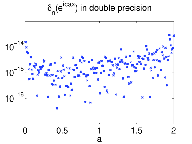
Figure 1: The quadrature error vs $|\lambda_{n}|$, with $c=1000$ and $n=682$. Here $\lambda_{n}=\mbox{\text{\rm{-.60352E-15}}}$.

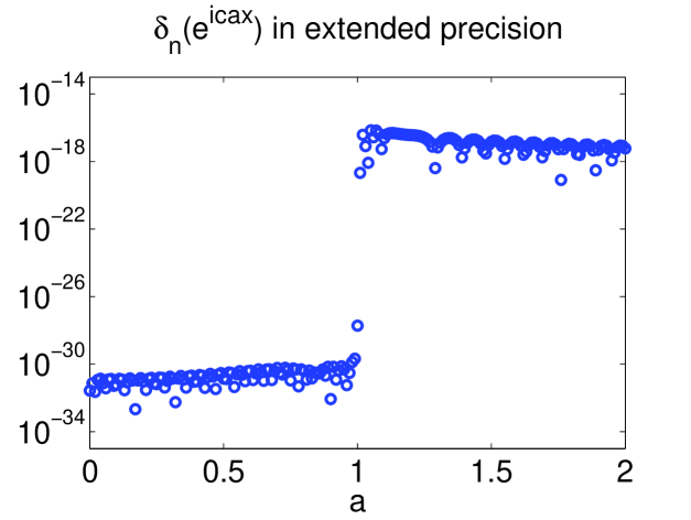
Figure 2: The quadrature error vs $|\lambda_{n}|$, with $c=1000$ and $n=682$. Here $\lambda_{n}=\mbox{\text{\rm{-.60352E-15}}}$.

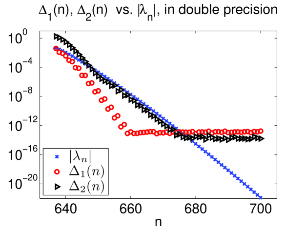
Figure 3: The maximal quadrature errors $\Delta_{1}(n),\Delta_{2}(n)$ vs $|\lambda_{n}|$, with $c=1000$.

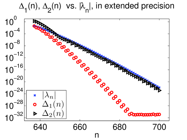
Figure 4: The maximal quadrature errors $\Delta_{1}(n),\Delta_{2}(n)$ vs $|\lambda_{n}|$, with $c=1000$.

Here we demonstrate the performance of the quadrature rule $S_{n}$ (see (101) in Section 4) on exponential functions. We proceed as follows. We choose, more or less arbitrarily, the band limit $c$ and the prolate index $n$. Next, we evaluate the quadrature nodes $t_{1},\dots,t_{n}$ and the quadrature weights $W_{1},\dots,W_{n}$ via the algorithms of Sections 5.3,  5.4, respectively. Also, we evaluate $|\lambda_{n}|$ via the algorithm in Section 5.2. Then, we choose a real number $0\leq a\leq 2$, and evaluate the integral of $e^{icax}$ over $-1\leq x\leq 1$ via the formula

$$\int_{-1}^{1}e^{iacx}\;dx=\int_{-1}^{1}\cos(acx)\;dx=\frac{2\sin(ac)}{ac}.$$ (159)

Also, we use $S_{n}$ to approximate (159) via the formula

$$\int_{-1}^{1}e^{iacx}\;dx\approx\sum_{j=1}^{n}e^{icat_{j}}\cdot W_{j}$$ (160)

(see (102) in Section 4). Finally, we evaluate the quadrature error $\delta_{n}(e^{iacx})$ via the formula

$$\delta_{n}(e^{iacx})=\left|\frac{2\sin(ac)}{ac}-\sum_{j=1}^{n}e^{icat_{j}}\cdot W_{j}\right|$$ (161)

(see (103) in Section 4).

In Figure 1, we display the results of this experiment. The band limit and the prolate index were chosen to be, respectively, $c=1000$ and $n=682$. For this choice of parameters, $\lambda_{n}=$ -.60352E-15. In this figure, we plot the quadrature error (161) as a function of the real parameter $a$, for $0\leq a\leq 2$, on the logarithmic scale. The calculations are carried out in double precision.

We make the following observations from Figure 1. The quadrature error is essentially zero up to machine precision $\varepsilon$, for all real $0\leq a\leq 2$. In other words, for this choice of parameters, the quadrature rule $S_{n}$ integrates the functions of the form $f(x)=e^{icax}$ with $0\leq a\leq 1$ exactly, for all practical purposes. It is perhaps surprising, however, that such functions are integrated exactly via $S_{n}$ even when $1<a\leq 2$. In other words, the quadrature rule $S_{n}$ (corresponding to band limit $c$ and $|\lambda_{n}|\approx\varepsilon$) integrates exactly the exponential functions with the band limit up to $2c$.

To get a clearer picture, we repeat this experiment in extended precision. In Figure 2, we plot the quadrature error (161) as a function of the real parameter $a$, for $0\leq a\leq 2$, on the logarithmic scale. In other words, Figure 2 is a version of Figure 1 in extended precision.

We make the following observations from Figure 2. If $0\leq a\leq 1$, then the quadrature rule $S_{n}$ integrates the functions of the form $f(x)=e^{icax}$ up to the error of order $|\lambda_{n}|^{2}$ (in Figure 1 we used double precision calculations and thus did not have enough digits to see this phenomenon). On the other hand, for $1<a\leq 2$ the quadrature rule $S_{n}$ integrates such functions up to the error roughly $|\lambda_{n}|$. In other words, the quadrature rule $S_{n}$ (corresponding to band limit $c$ and $|\lambda_{n}|\approx\varepsilon$) integrates the functions of band limit up to $c$ up to $\varepsilon^{2}$ (rather than $\varepsilon$); on the other hand, the functions of band limit between $c$ and $2c$ are integrated up to $\varepsilon$.

Explanation. These observations admit the following (somewhat imprecise) explanation (see [25], [26] for more details). Suppose that $a\geq 0$ is a real number. Due to (27) and Theorem 1 in Section 3.1,

$$e^{iacx}=\sum_{m=0}^{\infty}\lambda_{m}\psi_{m}(a)\psi_{m}(x),$$ (162)

for all real $-1\leq x\leq 1$. Moreover,

$$\int_{-1}^{1}e^{iacx}\;dx=\frac{2\sin(ac)}{ac}=\sum_{m=0}^{\infty}\lambda_{m}^{2}\psi_{m}(a)\psi_{m}(0).$$ (163)

We combine (161), (162), (163) to obtain

$$\frac{2\sin(ac)}{ac}-\sum_{j=1}^{n}W_{j}\cdot e^{icat_{j}}=\sum_{m=0}^{\infty}\lambda_{m}\psi_{m}(a)\left(\lambda_{m}\psi_{m}(0)-\sum_{j=1}^{n}W_{j}\psi_{m}(t_{j})\right).$$ (164)

Obviously, the quadrature error $\delta_{n}(\psi_{m})$ (see (173)) is zero for odd $m$. Also, $\delta_{n}(\psi_{m})$ rapidly increases as a function of even $0\leq m<n$; moreover, $\delta_{n}(\psi_{m})$ is of order $|\lambda_{n}|$ when $m<n$ is an even integer close to $n$ (see Conjectures 2, 3 in Section 7.1 and Theorem 14 in Section 4.1). Therefore, roughly speaking,

$$\sum_{m=0}^{n-1}\lambda_{m}\psi_{m}(a)\left(\lambda_{m}\psi_{m}(0)-\sum_{j=1}^{n}W_{j}\psi_{m}(t_{j})\right)\approx|\lambda_{n}|^{2}\cdot\psi_{n-1}(a).$$ (165)

On the other hand, due to the fast decay of $|\lambda_{m}|$ (see Theorems 2, 7 in Section 3.1),

$$\sum_{m=n}^{\infty}\lambda_{m}\psi_{m}(a)\left(\lambda_{m}\psi_{m}(0)-\sum_{j=1}^{n}W_{j}\psi_{m}(t_{j})\right)\approx|\lambda_{n}|^{2}.$$ (166)

Finally, the following approximate formula appears in [25], [26], in a slightly different form: suppose that $n>0$ is an integer, that $\chi_{n}>c^{2}$, and that $0\leq a\leq 2$ is a real number. Then,

$$|\psi_{n}(a)|=\begin{cases}O\left(\sqrt{n}\right),&0\leq a\leq 1,\\ O\left(|\lambda_{n}|^{-1}\right),&1<a\leq 2.\end{cases}$$ (167)

It follows from the combination of (165), (166), (167) that the quadrature error (161) is expected to be of the order $|\lambda_{n}|^{2}\cdot\sqrt{n}$, if $0\leq a\leq 1$. On the other hand, the quadrature error (161) is expected to be of the order $|\lambda_{n}|$, if $1<a\leq 2$. Figures 1, 2, 3, 4 support these somewhat vague conclusions.

We summarize this crude analysis, supported by the observations above, in the following conjecture about the quadrature error (161) for $0\leq a\leq 2$.

Conjecture 1.

Suppose that $c>0$ and $a\geq 0$ are real numbers, and that $n>2c/\pi$ is an integer. Suppose also that $\delta_{n}(e^{icax})$ is defined via (103) in Definition 2 in Section 4. If $0\leq a\leq 1$, then

$$\delta_{n}\left(e^{icax}\right)=\left|\int_{-1}^{1}e^{icax}\;dx-\sum_{j=1}^{n}e^{icat_{j}}\cdot W_{j}\right|\approx|\lambda_{n}|^{2}\cdot\sqrt{n},$$ (168)

where $\lambda_{n}$ is that of (27) in Section 3.1. If, on the other hand, $1<a\leq 2$, then

$$\delta_{n}\left(e^{icax}\right)=\left|\int_{-1}^{1}e^{icax}\;dx-\sum_{j=1}^{n}e^{icat_{j}}\cdot W_{j}\right|\approx|\lambda_{n}|.$$ (169)

We repeat the above experiment with various values of $n$, and plot the results in Figure 3. This figure also corresponds to band limit $c=1000$. We plot the following three quantities as functions of the prolate index $n$ that varies between $637\approx 2c/\pi$ and $700$. First, we plot $|\lambda_{n}|$. Second, we plot the maximal quadrature error $\Delta_{1}(n)$ defined via the formula

$$\Delta_{1}(n)=\max_{0\leq a\leq 1}\delta_{n}(e^{icax})=\max_{0\leq a\leq 1}\left|\frac{2\sin(ac)}{ac}-\sum_{j=1}^{n}e^{icat^{(n)}_{j}}\cdot W^{(n)}_{j}\right|,$$ (170)

where $t_{1}^{(n)},\dots,t_{n}^{(n)}$ and $W_{1}^{(n)},\dots,W_{n}^{(n)}$ are, respectively, the notes and weights of the quadrature rule $S_{n}$ (see (101) in Section 4). Finally, we plot the maximal quadrature error $\Delta_{2}(n)$ defined via the formula

$$\Delta_{2}(n)=\max_{1<a\leq 2}\delta_{n}(e^{icax})=\max_{1<a\leq 2}\left|\frac{2\sin(ac)}{ac}-\sum_{j=1}^{n}e^{icat^{(n)}_{j}}\cdot W^{(n)}_{j}\right|.$$ (171)

We observe that in (170) the parameter $a$ varies between $0$ and $1$, and in (171) the parameter $a$ varies between $1$ and $2$. In other words, $\Delta_{1}(n)$ is the maximal quadrature errors of $S_{n}$ for the exponential functions of band limits up to $c$, and $\Delta_{2}(n)$ is the maximal quadrature error of $S_{n}$ for the exponential functions of band limit between $c$ and $2c$.

We make the following observations from Figure 3. As long as $|\lambda_{n}|$ is less than roughly $10^{-7}\approx\sqrt{\varepsilon}$ (with $\varepsilon$ the machine precision), $\Delta_{1}(n)$ is roughly equal to $|\lambda_{n}|^{2}$. On the other hand, $\Delta_{1}(n)$ is zero up to machine precision once $|\lambda_{n}|>10^{-7}$. These observations are in agreement with Conjecture 1 above.

We also observe that $\Delta_{2}(n)$ is roughly of order $|\lambda_{n}|$, as long as $|\lambda_{n}|>\varepsilon$. On the other hand, when $\lambda_{n}$ is zero to machine precision, so is $\Delta_{2}(n)$ (see Conjecture 1).

We repeat this experiment in extended precision, and plot the results in Figure 4. In other words, Figure 4 is a version of Figure 3 in extended precision. We observe the same phenomenon: $\Delta_{1}(n)$ is of order $|\lambda_{n}|^{2}$, and $\Delta_{2}(n)$ is of order $|\lambda_{n}|$ (as long as we do not run out of digits to see it; if, for example, $|\lambda_{n}|$ is below the machine zero so are both $\Delta_{1}(n)$ and $\Delta_{2}(n)$). In other words, the quadrature error of $S_{n}$ for exponential functions with band limit up to $c$ is of order $|\lambda_{n}|^{2}$, and the quadrature error of $S_{n}$ for exponential functions with band limit between $c$ and $2c$ is of order $|\lambda_{n}|$, which supports Conjecture 1.

7 Numerical Illustration of Analysis in Section 4

In this section, we illustrate the analytical results from Section 4 and the performance of the algorithms described in Section 5. All the calculations were implemented in FORTRAN (the Lahey 95 LINUX version), and carried out in double precision. Extended precision calculations were used for comparison and verification (in extended precision, the floating point numbers are 128 bits long, as opposed to 64 bits in double precision).

7.1 Quadrature Error and its Relation to $|\lambda_{n}|$

In this section, we describe several numerical experiments that illustrate the quadrature error (see (101), (103) in Section 4) and its relation to $|\lambda_{n}|$.

$m$	$\displaystyle\lambda_{m}\psi_{m}(0)$	$\displaystyle\delta_{n}(\psi_{m}),\text{ double precision }$	$\displaystyle\delta_{n}(\psi_{m}),\text{ extended precision }$
0	0.70669E+00	0.44409E-15	0.33258E-26
2	0.49581E+00	0.16653E-15	0.22426E-25
4	0.42581E+00	0.13323E-14	0.26756E-23
6	0.38527E+00	0.21649E-14	0.19692E-21
8	0.35695E+00	0.22760E-14	0.91546E-20
10	0.33516E+00	0.16653E-14	0.29148E-18
12	0.31730E+00	0.23870E-14	0.88165E-17
14	0.30201E+00	0.24980E-14	0.21007E-15
16	0.28844E+00	0.11102E-14	0.35574E-14
18	0.27604E+00	0.59230E-13	0.57028E-13
20	0.26435E+00	0.83716E-12	0.83954E-12
22	0.25299E+00	0.89038E-11	0.89011E-11
24	0.24150E+00	0.76862E-10	0.76864E-10
26	0.22919E+00	0.65870E-09	0.65870E-09
28	0.21377E+00	0.45239E-08	0.45239E-08
30	0.18075E+00	0.19826E-07	0.19826E-07
32	0.10038E+00	0.68548E-07	0.68548E-07
34	0.27988E-01	0.33810E-06	0.33810E-06
36	0.49822E-02	0.27232E-05	0.27232E-05
38	0.70503E-03	0.22754E-04	0.22754E-04

Table 1: Illustration of Theorem 14 with $c=50$ and $n=40$. For these parameters, $\lambda_{n}=\mbox{\text{\rm{0.12915E-03}}}$. See Experiment 2.

Experiment 2.

Here we illustrate Theorem  14 in Section 4.1. We choose, more or less arbitrarily, band limit $c$ and prolate index $n$. We evaluate $\chi_{n}$, $\lambda_{n}$ and the quadrature rule $S_{n}$ defined via (101) in Section 4 via the algorithms of Sections 5.1, 5.2, 5.3, 5.4, respectively. Then, we choose an even integer $0\leq m<n$, and evaluate $\lambda_{m}$, $\psi_{m}(0)$, and $\psi_{m}(t_{j})$ for all $j=1,\dots,n$, via the algorithms of Sections 5.1, 5.2. All the calculations are carried out in double precision.

We display the results of this experiment in Table 1. The data in this table correspond to $c=50$ and $n=40$. Table 1 has the following structure. The first column contains the even integer $m$, that varies between $0$ and $n-2$. The second column contains $\lambda_{m}\psi_{m}(0)$ (we observe that

$$\lambda_{m}\psi_{m}(0)=\int_{-1}^{1}\psi_{m}(t)\;dt,$$ (172)

due to (27) in Section 3.1). The third column contains the quadrature error

$$\delta_{n}(\psi_{m})=\left|\lambda_{m}\psi_{m}(0)-\sum_{j=1}^{n}\psi_{m}(t_{j})\cdot W_{j}\right|$$ (173)

(see (103) in Section 4), computed in double precision.

Then, we repeat all the calculations in extended precision; the last column of Table 1 contains $\delta_{n}(\psi_{m})$ defined via (173) (the same quantity as in the third column evaluated in extended precision).

We make the following observations from Table 1. We note that $\lambda_{m}\psi_{m}(0)$ is always positive and monotonically decreases with $m$. We also note that $\delta_{n}(\psi_{m})$ (evaluated in double precision) is close to the machine accuracy for small $m$, and grows up to $\approx 2\cdot 10^{-5}$ for $m=38$. Also, $\delta_{n}(\psi_{m})$ is bounded by $|\lambda_{n}|$, for all values of $m$ in Table 1 (in this case, $|\lambda_{n}|=$ 0.12915E-03). Finally, $\delta_{n}(\psi_{m})$ (evaluated in extended precision) is a monotonically increasing function of even $0\leq m<n$ (obviously, $\delta_{n}(\psi_{m})=0$ for odd $m$).

We summarize these observations in the following conjecture. We have not fully investigated the phenomenon described in this conjecture; see, however, Theorem 14 in Section 4.1, Conjecture 3 below, Figure 5 and Table 3 (see also [25], [26] for additional details and analysis).

Conjecture 2.

Suppose that $c>1$ is a real number, that $n>2c/\pi$ is an integer, and that the quadrature rule $S_{n}$ is defined via (101) in Section 4. Then, the quadrature error $\delta_{n}(\psi_{m})$ defined via (173) above is a monotonically increasing function of even $0\leq m<n$. Moreover, in double precision calculations $\delta_{n}(\psi_{m})$ is zero up to machine precision for all $0\leq m<2c/\pi$.

In (106) in Theorem 14, we provide an upper bound on $\delta_{n}(\psi_{m})$. This bound does not depend on $m$; more specifically, for every $m=0,\dots,n-1$,

$$\delta_{n}(\psi_{m})=\left|\lambda_{m}\psi_{m}(0)-\sum_{j=1}^{n}\psi_{m}(t_{j})\cdot W_{j}\right|\leq|\lambda_{n}|\cdot\left(24\cdot\log\left(\frac{1}{|\lambda_{n}|}\right)+6\cdot\chi_{n}\right).$$ (174)

On the other hand, according to Table 1 the quadrature error $\delta_{n}(\psi_{m})$ is bounded by $|\lambda_{n}|$ alone, for all even $0\leq m<n$ (obviously, $\delta_{n}(\psi_{m})=0$ for all odd $m$).

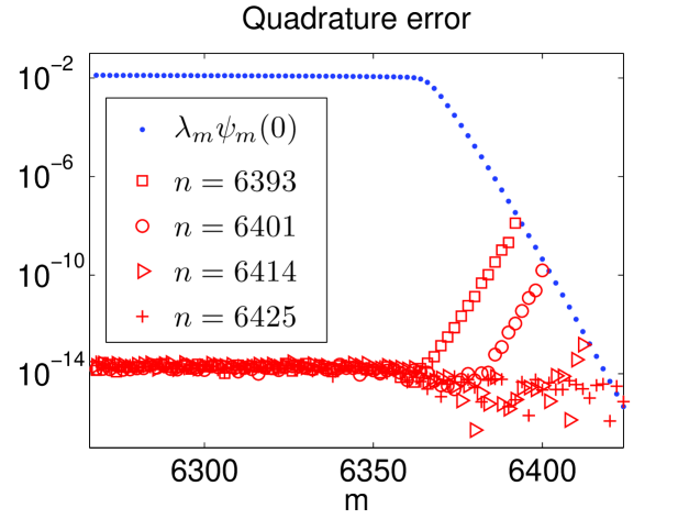
Figure 5: The quadrature error $\displaystyle\delta_{n}(\psi_{m})=\left|\int_{-1}^{1}\psi_{m}(t)\;dt-\sum_{j=1}^{n}\psi_{m}(t_{j})\cdot W_{j}\right|$ as a function of even $m<n$, for four different values of $n$ and $c=10000$, vs. $\displaystyle\lambda_{m}\psi_{m}(0)$. See Experiment 2.

In Figure 5, we display the results of the same experiment with different choice of parameters $c$ and $n$. Namely, we choose $c=10000$ and plot $\lambda_{m}\psi_{m}(0)$ as a function of even $0\leq m<6425$, on the logarithmic scale (solid line). In addition, we plot the quadrature error $\delta_{n}(\psi_{m})$ as a function of $m$, for four different values of $n$: $n=6393$ (dashed line), $n=6401$ (circles), $n=6414$ (triangles), and $n=6425$ (pluses). The corresponding values of $|\lambda_{n}|$ are displayed in Table 2.

$n$	6393	6401	6414	6425
$|\lambda_{n}|$	0.43299E-07	0.54119E-09	0.33602E-12	0.52616E-15

Table 2: Values of $|\lambda_{n}|$ for $c=10000$ and different choices of $n$.

We make the following observations from Figure 5. First, the quantities $\lambda_{m}\psi_{m}(0)$ are of the same order of magnitude for all $m<2c/\pi$, and decay rapidly with $m$ for $m>2c/\pi$. Also, for each value of $n$, the quadrature error $\delta_{n}(\psi_{m})$ is essentially zero for all $m<2c/\pi$ and increases rapidly with $m$ for $m>2c/\pi$. Nevertheless, $\delta_{n}(\psi_{m})$ is always bounded from above by $|\lambda_{n}|$, for each $n$ and each $m<n$. See also Tables 1, 3 and Conjecture 3 below.

$c$	$n$	$m$	$\lambda_{m}\psi_{m}(0)$	$\displaystyle\int_{-1}^{1}\psi_{m}(t)\;dt-\sum_{j=1}^{n}\psi_{m}(t_{j})\cdot W_{j}$	$|\lambda_{n}|$
250	179	178	0.28699E-07	-.52496E-08	0.18854E-07
250	184	182	0.68573E-09	-.38341E-10	0.16130E-09
250	188	186	0.14108E-10	-.68758E-12	0.30500E-11
500	339	338	0.52368E-07	-.13473E-07	0.40938E-07
500	345	344	0.37412E-09	-.86136E-10	0.27418E-09
500	350	348	0.12148E-10	-.99816E-12	0.35537E-11
1000	659	658	0.42709E-07	-.14354E-07	0.38241E-07
1000	665	664	0.51665E-09	-.15924E-09	0.43991E-09
1000	671	670	0.52494E-11	-.15024E-11	0.42815E-11
2000	1297	1296	0.41418E-07	-.17547E-07	0.41740E-07
2000	1304	1302	0.77185E-09	-.15036E-09	0.37721E-09
2000	1311	1310	0.31078E-11	-.11386E-11	0.28754E-11
4000	2572	2570	0.54840E-07	-.15493E-07	0.33682E-07
4000	2579	2578	0.43032E-09	-.20771E-09	0.46141E-09
4000	2587	2586	0.28193E-11	-.12805E-11	0.29164E-11
8000	5119	5118	0.43268E-07	-.26751E-07	0.52899E-07
8000	5128	5126	0.50230E-09	-.16395E-09	0.33442E-09
8000	5136	5134	0.50508E-11	-.15448E-11	0.32132E-11
16000	10213	10212	0.42725E-07	-.30880E-07	0.56568E-07
16000	10222	10220	0.69663E-09	-.28201E-09	0.52821E-09
16000	10231	10230	0.34472E-11	-.22162E-11	0.42902E-11

Table 3: Relation between the quadrature error and $|\lambda_{n}|$. See Experiment 2.

We repeat the experiment above with several other values of band limit $c$ and prolate index $n$. The results are displayed in Table 3. This table has the following structure. The first and second column contain, respectively, the band limit $c$ and the prolate index $n$. The third column contains the even integer $0\leq m<n$ (the values of $m$ were chosen to be close to $n$). The fourth column contains $\lambda_{m}\psi_{m}(0)$. The fifth column contains (173). The last column contains $|\lambda_{n}|$.

We make the following observations from Table 3. First, for each of the seven values of $c$, the three indices $n$ were chosen in such a way that $|\lambda_{n}|$ is between $10^{-12}$ and $10^{-7}$. The values of the band limit $c$ vary between $250$ (the first three rows) and $16000$ (the last three rows). For each $n$, the value of $m$ is chosen to be the largest even integer below $n$. This choice of $m$ yields the smallest $\lambda_{m}\psi_{m}(0)$ and the largest quadrature error $\delta_{n}(\psi_{m})$ among all $m<n$ (see also Table 1 and Figure 5). Obviously, for this choice of $m$ the eigenvalues $\lambda_{m}$ and $\lambda_{n}$ are roughly of the same order of magnitude. We also observe that for all the values of $c,n,m$, the quadrature error $\delta_{n}(\psi_{m})$ is bounded from above by $|\lambda_{n}|$ (and is roughly equal to $|\lambda_{n}|/2$). In other words, the upper bound on $\delta_{n}(\psi_{m})$ provided by Theorem 14 (see (174)) is somewhat overcautious.

We summarize these observations in the following conjecture.

Conjecture 3.

Suppose that $c>0$ is a positive real number, and that $n>2c/\pi$ is an integer. Suppose also that $0\leq m<n$ is an integer. Suppose furthermore that $\delta_{n}(\psi_{m})$ is defined via (103) in Definition 2 in Section 4. Then,

$$\delta_{n}(\psi_{m})=\left|\int_{-1}^{1}\psi_{m}(s)\;ds-\sum_{j=1}^{n}\psi_{m}(t_{j})\cdot W_{j}\right|\leq|\lambda_{n}|,$$ (175)

where $\lambda_{n}$ is that of (27) in Section 3.1.

Remark 37.

The inequality (175) in Conjecture 3 is stronger than the inequality (106) in Theorem 14. On the other hand, as opposed to Theorem 14, Conjecture 3 has been only supported by numerical evidence.

Experiment 3.

Here we illustrate Theorems 15, 16 in Section 4.2. We proceed as follows. We choose, more or less arbitrarily, the band limit $c>0$ and the accuracy parameter $\varepsilon>0$. Then, we use the algorithm of Section 5.2 to find the minimal integer $m$ such that $|\lambda_{m}|<\varepsilon$. In other words, we define the integer $n_{1}(\varepsilon)$ via the formula

$$n_{1}(\varepsilon)=\min\left\{m\geq 0\;:\;|\lambda_{m}|<\varepsilon\right\}.$$ (176)

Also, we find the minimal integer such that the right-hand side of (106) in Theorem 14 in Section 4.1 is less that $\varepsilon$. In other words, we define the integer $n_{2}(\varepsilon)$ via the formula

$$n_{2}(\varepsilon)=\min\left\{m\geq 0\;:\;|\lambda_{m}|\cdot\left(24\cdot\log\left(\frac{1}{|\lambda_{m}|}\right)+6\cdot\chi_{m}\right)<\varepsilon\right\}.$$ (177)

Next, we evaluate the integer $n_{3}(\varepsilon)$ via the formula (110) in Theorem 15. In other words,

$$n_{3}(\varepsilon)=\text{floor}\left(\frac{2c}{\pi}+\frac{\alpha(\varepsilon)}{2\pi}\cdot\log\left(\frac{16ec}{\alpha(\varepsilon)},\right)\right)$$ (178)

where $\alpha(\varepsilon)$ is defined via (109) in Theorem 15. Finally, we evaluate the integer $n_{4}(\varepsilon)$ via the right-hand side of (115) in Theorem 16. In other words,

$$n_{4}(\varepsilon)=\text{floor}\left(\frac{2c}{\pi}+\left(10+\frac{3}{2}\cdot\log(c)+\frac{1}{2}\cdot\log\frac{1}{\varepsilon}\right)\cdot\log\left(\frac{c}{2}\right)\right).$$ (179)

In both (178) and (179), $\text{floor}(a)$ denotes the integer part of a real number $a$.

$c$	$\varepsilon$	$n_{1}(\varepsilon)$	$n_{2}(\varepsilon)$	$n_{3}(\varepsilon)$	$n_{4}(\varepsilon)$	$|\lambda_{n_{1}(\varepsilon)}|$	$|\lambda_{n_{2}(\varepsilon)}|$
250	$10^{-10}$	184	198	277	303	0.60576E-10	0.86791E-16
250	$10^{-25}$	216	227	326	386	0.31798E-25	0.14863E-30
250	$10^{-50}$	260	270	393	525	0.28910E-50	0.75155E-56
500	$10^{-10}$	346	362	460	488	0.49076E-10	0.60092E-16
500	$10^{-25}$	382	397	520	583	0.54529E-25	0.19622E-31
500	$10^{-50}$	433	446	607	742	0.82391E-50	0.38217E-56
1000	$10^{-10}$	666	687	803	834	0.95582E-10	0.92947E-17
1000	$10^{-25}$	707	725	875	942	0.97844E-25	0.14241E-31
1000	$10^{-50}$	767	783	981	1120	0.39772E-50	0.56698E-57
2000	$10^{-10}$	1305	1330	1467	1500	0.95177E-10	0.25349E-17
2000	$10^{-25}$	1351	1373	1550	1619	0.86694E-25	0.27321E-32
2000	$10^{-50}$	1418	1438	1675	1818	0.88841E-50	0.22795E-57
4000	$10^{-10}$	2581	2610	2768	2804	0.70386E-10	0.64396E-18
4000	$10^{-25}$	2632	2658	2862	2935	0.57213E-25	0.53827E-33
4000	$10^{-50}$	2707	2730	3007	3154	0.56712E-50	0.88819E-58
8000	$10^{-10}$	5130	5163	5344	5383	0.59447E-10	0.22821E-18
8000	$10^{-25}$	5185	5216	5450	5526	0.87242E-25	0.16237E-33
8000	$10^{-50}$	5268	5296	5614	5765	0.95784E-50	0.23927E-58
16000	$10^{-10}$	10225	10264	10468	10509	0.63183E-10	0.37516E-19
16000	$10^{-25}$	10285	10321	10585	10664	0.85910E-25	0.41416E-34
16000	$10^{-50}$	10377	10409	10769	10923	0.51912E-50	0.56250E-59
32000	$10^{-10}$	20413	20457	20686	20730	0.62113E-10	0.12818E-19
32000	$10^{-25}$	20478	20519	20815	20897	0.78699E-25	0.12197E-34
32000	$10^{-50}$	20577	20615	21018	21176	0.96802E-50	0.15816E-59
64000	$10^{-10}$	40786	40837	41092	41139	0.89344E-10	0.28169E-20
64000	$10^{-25}$	40857	40903	41232	41318	0.66605E-25	0.39212E-35
64000	$10^{-50}$	40964	41008	41454	41616	0.85451E-50	0.28036E-60
$10^{6}$	$10^{-10}$	636669	636747	637115	637174	0.79326E-10	0.13385E-22
$10^{6}$	$10^{-25}$	636759	636832	637301	637400	0.77413E-25	0.15758E-37
$10^{6}$	$10^{-50}$	636899	636968	637600	637778	0.69235E-50	0.15801E-62

Table 4: Illustration of Theorems 15, 16. See Experiment 3.

We display the results of this experiment in Table 4. This table has the following structure. The first column contains the band limit $c$. The second column contains the accuracy parameter $\varepsilon$. The third column contains $n_{1}(\varepsilon)$ defined via (176). The fourth column contains $n_{2}(\varepsilon)$ defined via (177). The fifth column contains $n_{3}(\varepsilon)$ defined via (178). The sixth column contains $n_{4}(\varepsilon)$ defined via (179). The seventh column contains $|\lambda_{n_{1}(\varepsilon)}|$. The last column contains $|\lambda_{n_{2}(\varepsilon)}|$.

Suppose that $c>0$ is a band limit, and $n>0$ is an integer. We define the real number $Q(c,n)$ via the formula

$$Q(c,n)=\max\left\{\delta_{n}(\psi_{m})=\left|\int_{-1}^{1}\psi_{m}(t)\;dt-\sum_{j=1}^{n}\psi_{m}(t_{j})\cdot W_{j}\right|\;:\;0\leq m\leq n-1\right\},$$ (180)

where $t_{1},\dots,t_{n}$ and $W_{1},\dots,W_{n}$ are defined, respectively, via (98), (100) in Definition 2 in Section 4. In other words, $Q(c,n)$ is the maximal error to which the quadrature rule $S_{n}$ defined via (101) integrates the first $n$ PSWFs.

We make the following observations from Table 4. We observe that $Q(c,n_{1}(\varepsilon))<\varepsilon$, due to the combination of Conjecture 3 in Section 7.1 and (176), (180). In other words, numerical evidence suggests that the quadrature rule $S_{n_{1}(\varepsilon)}$ integrates the first $n_{1}(\varepsilon)$ PSWFs up to an error less than $\varepsilon$ (see Remark 37). On the other hand, we combine Theorem 14 in Section 4.1 with (177), (180), to conclude that the quadrature rule $S_{n_{2}(\varepsilon)}$ has been rigorously proven to integrate the first $n_{2}(\varepsilon)$ PSWFs up to an error less than $\varepsilon$. In both Theorem 14 and Conjecture 3, we establish upper bounds on $Q(c,n)$ in terms of $|\lambda_{n}|$. The ratio of $|\lambda_{n_{1}(\varepsilon)}|$ to $|\lambda_{n_{2}(\varepsilon)}|$ is quite large: from about $10^{6}$ for $c=250$ and $\varepsilon=10^{-10},10^{-25},10^{-50}$ (see the first three rows in Table 4), to about $10^{10}$ for $c=64000$ and $\varepsilon=10^{-10},10^{-25},10^{-50}$, to about $5\cdot 10^{12}$ for $c=10^{6}$ and $\varepsilon=10^{-10},10^{-25},10^{-50}$, (see the last six rows in Table 4). On the other hand, the difference between $n_{2}(\varepsilon)$ and $n_{1}(\varepsilon)$ is fairly small; for example, for $\varepsilon=10^{-50}$, this difference varies from 10 for $c=250$ to $23$ for $c=4000$, to merely $44$ for $c=64000$ and $69$ for as large $c$ as $c=10^{6}$.

As opposed to $n_{1}(\varepsilon)$ and $n_{2}(\varepsilon)$, the integer $n_{3}(\varepsilon)$ is computed via the explicit formula (178) that depends only on $c$ and $\varepsilon$ (rather than on $|\lambda_{n}|$ and $\chi_{n}$, that need to be evaluated numerically); this formula appears in Theorem 15. The convenience of (178) vs. (176), (177) comes at a price: for example, for $\varepsilon=10^{-50}$, the difference between $n_{3}(\varepsilon)$ and $n_{2}(\varepsilon)$ is equal to 123 for $c=250$, to 446 for $c=64000$, and to 632 for $c=10^{6}$. However, the difference $n_{3}(\varepsilon)-n_{2}(\varepsilon)$ is rather small compared to $c$: for example, for $\varepsilon=10^{-50}$, this difference is roughly $4\cdot\left(\log(c)\right)^{2}$, for all values of $c$ in Table 4.

Furthermore, we observe that $n_{4}(\varepsilon)$ is computed via the explicit formula (179) that depends only on $c$ and $\varepsilon$. This formula can be viewed as a simplified version of (178) (see Theorems 15, 16); in particular, $n_{4}(\varepsilon)$ is greater than $n_{3}(\varepsilon)$, for all $c$ and $\varepsilon$.

We summarize these observations as follows. Suppose that the band limit $c>0$ and the accuracy parameter $\varepsilon>0$ are given. According to Theorem 15, for any $n\geq n_{3}(\varepsilon)$ the quadrature rule $S_{n}$ defined via (101) in Section 4 is guaranteed to integrate the first $n$ PSWFs to precision $\varepsilon$ (see Definition 1 in Section 2.1). On the other hand, numerical evidence (see Experiment 2) suggests that the choice $n\geq n_{3}(\varepsilon)$ is overly cautious for this purpose; more specifically, $S_{n}$ integrates the first $n$ PSWFs to precision $\varepsilon$ for every $n$ between $n_{1}(\varepsilon)$ and $n_{3}(\varepsilon)$ as well. In this experiment, we observed that the difference between the ”theoretical” bound $n_{3}(\varepsilon)$ and ”empirical” bound $n_{1}(\varepsilon)$ is of order $\left(\log(c)\right)^{2}$, and, in particular, is relatively small compared to both $n_{1}(\varepsilon)$ and $n_{3}(\varepsilon)$ (which are of order $c$).

Finally, we observe that

$$n_{1}(\varepsilon)<\frac{2c}{\pi}+\frac{2}{\pi^{2}}\cdot\left(\log c\right)\cdot\log\frac{1}{\varepsilon},$$ (181)

for all the values of $c$ and $\varepsilon$ in Table 4. Combined with some additional numerical experiments by the authors, this observation leads to the following conjecture (see also Theorem 7 in Section 3.1 for a rigorously proven and more precise statement).

Conjecture 4.

Suppose that $c>1$ and $0<\varepsilon<1$ are real numbers. Suppose also that $n>0$ is an integer, and that

$$n>\frac{2c}{\pi}+10+\frac{2}{\pi^{2}}\cdot\left(\log c\right)\cdot\log\frac{1}{\varepsilon}.$$ (182)

Then,

$$|\lambda_{n}|<\varepsilon,$$ (183)

where $\lambda_{n}$ is that of (27) in Section 3.1.

7.2 Quadrature Weights

In this section, we illustrate the results of Section 4.3 and the algorithms of Section 5.4.

$j$	$\widehat{W}_{j}$	$\widehat{W_{j}}-\widetilde{W}_{j}$	$\widehat{W}_{j}-\frac{\widehat{W}_{(n+1)/2}\left(\psi_{n}^{\prime}(0)\right)^{2}}{\left(\psi_{n}^{\prime}(t_{j})\right)^{2}\cdot\left(1-t_{j}^{2}\right)}$
1	0.7602931556894E-02	0.00000E+00	-.55796E-11
2	0.1716167229714E-01	0.00000E+00	-.55504E-10
3	0.2563684665002E-01	0.00000E+00	-.21825E-12
4	0.3278512460580E-01	0.00000E+00	-.11959E-09
5	0.3863462966166E-01	0.16653E-15	0.82238E-11
6	0.4334940472363E-01	0.22204E-15	-.16247E-09
7	0.4713107235981E-01	0.22204E-15	0.11270E-10
8	0.5016785516291E-01	0.19429E-15	-.18720E-09
9	0.5261660773966E-01	0.26368E-15	0.10495E-10
10	0.5460119701692E-01	0.29837E-15	-.20097E-09
11	0.5621699326080E-01	0.17347E-15	0.81464E-11
12	0.5753664411864E-01	0.12490E-15	-.20866E-09
13	0.5861531690539E-01	0.10408E-15	0.55098E-11
14	0.5949490764741E-01	0.23592E-15	-.21301E-09
15	0.6020725336886E-01	0.13184E-15	0.31869E-11
16	0.6077650804037E-01	0.18041E-15	-.21545E-09
17	0.6122088420703E-01	0.48572E-16	0.14361E-11
18	0.6155390478472E-01	0.83267E-16	-.21675E-09
19	0.6178529976346E-01	0.11102E-15	0.36146E-12
20	0.6192162112196E-01	0.48572E-16	-.21732E-09
21	0.6196665001384E-01	0.00000E+00	0.00000E+00

Table 5: Quadrature weights (100) with $c=40$, $n=41$. $\lambda_{n}=\mbox{\text{\rm{i0.69857E-08}}}$. See Experiment 4.

Experiment 4.

In this experiment, we choose, more or less arbitrarily, band limit $c$ and prolate index $n$. Then, we compute $t_{1},\dots,t_{n}$ (see (98)) and $\psi_{n}^{\prime}(t_{1}),\dots,\psi_{n}^{\prime}(t_{n})$ via the algorithm of Section 5.3. Also, we evaluate $\psi_{n}(0),\psi_{n}^{\prime}(0)$ via the algorithm of Section 5.1. Next, compute approximations $\widetilde{W}_{1},\dots,\widetilde{W}_{n}$ to $W_{1},\dots,W_{n}$ via Algorithm 1 in Section 5.4 (in particular, $\widetilde{W}_{j}$ is evaluated via (150) for every $j=1,\dots,n$). Also, we compute approximations $\widehat{W}_{1},\dots,\widehat{W}_{n}$ to $W_{1},\dots,W_{n}$ via Algorithm 2 in Section 5.4. All the calculations are carried out in double precision.

We display the results of this experiment in Table 5. The data in this table correspond to $c=40$ and $n=41$. Table 5 has the following structure. The first column contains the weight index $j$, that varies between 1 and $(n+1)/2=21$. The second column contains $\widehat{W}_{j}$ ( an approximation to $W_{j}$ evaluated by Algorithm 2 in Section 5.4). The third column contains the difference between $\widehat{W}_{j}$ and $\widetilde{W}_{j}$ (evaluated via (150) by Algorithm 1). The last column contains the difference

$$\widehat{W}_{j}-\frac{\widehat{W}_{(n+1)/2}\cdot\left(\psi_{n}^{\prime}(0)\right)^{2}}{\left(\psi_{n}^{\prime}(t_{j})\right)^{2}\cdot\left(1-t_{j}^{2}\right)}$$ (184)

(see (125) in Remark 14).

In Figure 6, we plot the weights $W_{j}$ as a function of $j=1,\dots,n$. Each $W_{j}$ is plotted as a circle above the corresponding node $t_{j}$.

We make the following observations from Table 5. First, due to the combination of Theorems 17, 18 in Section 4.3, the value in the third column would be zero in exact arithmetic. We observe that, indeed, this value is zero up to the machine precision, which confirms Remarks 30, 35 in Section 5.4. (We note that, for $j=1,2,3,4$ and $j=21$, both $\widehat{W}_{j}$ and $\widetilde{W}_{j}$ are evaluated via (150), and hence the value in the corresponding rows is exactly zero). In particular, either of the two approximations $\widetilde{W}_{j},\widehat{W}_{j}$ can be used to evaluate $W_{j}$ to essentially machine precision.

We also observe that all of the weights $W_{1},\dots,W_{n}$ are positive (see Theorem 19 and Remark 13). Moreover, $W_{j}$ grow monotonically as $j$ increases to $(n+1)/2$. Finally, we observe that, for all $j=1,\dots,n$, the value (184) in the last column is of the order $|\lambda_{n}|$ (see Remark 14).

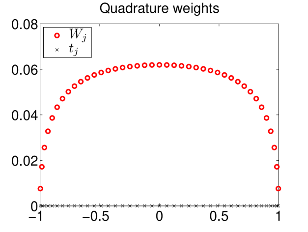
Figure 6: The quadrature weights $W_{1},\dots,W_{n}$ with $c=40$, $n=41$. See Experiment 4.

References

- [1] M. Abramowitz, I. A. Stegun, Handbook of Mathematical Functions with Formulas, Graphs and Mathematical Tables, Dover Publications, 1964.
- [2] W. Barth, R. S. Martin, J. H. Wilkinson, Calculation of the Eigenvalues of a Symmetric Tridiagonal Matrix by the Method of Bisection, Numerische Mathematik 9, 386-393, 1967.
- [3] C. J. Bouwkamp, On spheroidal wave functions of order zero, J. Math. Phys. 26, 79-92, 1947.
- [4] H. Cheng, N. Yarvin, V. Rokhlin, Non-linear Optimiuzation, Quadrature and Interpolation, SIAM J. Optim. 9, 901-23, 1999.
- [5] G. Dahlquist, A. Björk, Numerical Methods, Prentice-Hall Inc., 1974.
- [6] M.V. Fedoryuk, Asymptotic Analysis of Linear Ordinary Differential Equations, Springer-Verlag, Berlin (1993).
- [7] C. Flammer, Spheroidal Wave Functions, Stanford, CA: Stanford University Press, 1956.
- [8] Andreas Glaser, Xiangtao Liu, Vladimir Rokhlin, A fast algorithm for the calculation of the roots of special functions, SIAM J. Sci. Comput., 29(4):1420-1438 (electronic), 2007.
- [9] I.S. Gradshteyn, I.M. Ryzhik, Table of Integrals, Series, and Products, Seventh Edition, Elsevier Inc., 2007.
- [10] D. B. Hodge, Eigenvalues and Eigenfunctions of the Spheroidal Wave Equation, J. Math. Phys. 11, 2308-2312, 1970.
- [11] E. Isaacson, H. B. Keller, Analysis of Numerical Methods, New York: Wiley, 1966.
- [12] S. Karlin, W. J. Studden, Tchebycheff Systems with Applications in Analysis and Statistics, Wiley-Interscience, New York, 1966.
- [13] M. G. Krein, The Ideas of P. L. Chevyshev and A. A. Markov in the THeory of Limiting Values of Integrals, AM. Math. Soc. Trans., 12, 1-122, 1959.
- [14] H. J. Landau, H. O. Pollak, Prolate spheroidal wave functions, Fourier analysis, and uncertainty - II, Bell Syst. Tech. J. January 65-94, 1961.
- [15] H. J. Landau, H. Widom, Eigenvalue distribution of time and frequency limiting, J. Math. Anal. Appl. 77, 469-81, 1980.
- [16] J. Ma, V. Rokhlin, S. Wandzura, Generalized Gaussian Quadratures for Systems of Arbitrary Functions, SIAM J. Numer. Anal. 33, 971-96, 1996.
- [17] A. A. Markov, On the Limiting Values of Integrals in Connection with Interpolation, Zap. Imp. Akad. Nauk. Fiz.-Mat. Otd. (8) 6, no 5 (in Russian), 1898.
- [18] A. A. Markov, Selected Papers on Continued Fractions and the Theory of Functions Deviating Least From Zero, OGIZ: Moscow (in Russian), 1948.
- [19] Richard K. Miller, Anthony N. Michel, Ordinary Differential Equations, Dover Publications, Inc., 1982.
- [20] P. M. Morse, H. Feshbach, Methods of Theoretical Physics, New York McGraw-Hill, 1953.
- [21] A. Osipov, Certain inequalities involving prolate spheroidal wave functions and associated quantities, Appl. Comput. Harmon. Anal. (2012), http://dx.doi.org/10.1016/j.acha.2012.10.002 (in press).
- [22] A. Osipov, Certain inequalities involving prolate spheroidal wave functions and associated quantities, arXiv:1206.4056v1, 2012.
- [23] A. Osipov, Explicit upper bounds on the eigenvalues associated with prolate spheroidal wave functions, Yale CS Technical Report #1450, 2012.
- [24] A. Osipov, Certain upper bounds on the eigenvalues associated with prolate spheroidal wave functions, arXiv:1206.4541v1, 2012.
- [25] A. Osipov, V. Rokhlin, Detailed analysis of prolate quadratures and interpolation formulas, Yale CS Technical Report #1458, 2012.
- [26] A. Osipov, V. Rokhlin, Detailed analysis of prolate quadratures and interpolation formulas, arXiv:1208.4816v1, 2012.
- [27] A. Osipov, Evaluation of small elements of the eigenvectors of certain symmetric tridiagonal matrices with high relative accuracy, Yale CS Technical Report #1460, 2012.
- [28] A. Osipov, Evaluation of small elements of the eigenvectors of certain symmetric tridiagonal matrices with high relative accuracy, arXiv:1208.4906v1, 2012.
- [29] A. Papoulis, Signal Analysis, Mc-Graw Hill, Inc., 1977.
- [30] Vladimir Rokhlin, Hong Xiao, Approximate Formulae for Certain Prolate Spheroidal Wave Functions Valid for Large Value of Both Order and Band Limit.
- [31] W. Rudin, Real and Complex Analysis, Mc-Graw Hill Inc., 1970.
- [32] D. Slepian, Some comments on Fourier analysis, uncertainty, and modeling, SIAM Rev.(3) 379-93, 1983.
- [33] D. Slepian, H. O. Pollak, Prolate spheroidal wave functions, Fourier analysis, and uncertainty - I, Bell Syst. Tech. J. January 43-63, 1961.
- [34] D. Slepian, H. O. Pollak, Prolate spheroidal wave functions, Fourier analysis, and uncertainty - IV: extensions to many dimensions, generalized prolate spheroidal wave functions, Bell Syst. Tech. J. November 3009-57, 1964.
- [35] D. Slepian, Some asymptotic expansions for prolate spheroidal wave functions, J. Math. Phys. 44 99-140, 1965.
- [36] J. H. Wilkinson, Algebraic Eigenvalue Problem, Oxford University Press, New York, 1965.
- [37] H. Xiao, V. Rokhlin, N. Yarvin, Prolate spheroidal wavefunctions, quadrature and interpolation, Inverse Problems, 17(4):805-828, 2001.
- [38] N. Yarvin, V. Rokhlin, Generalized Gaussian Quadratures and Singular Value Decompositions of Integral Operators, SIAM J. Sci. Comput. 20, 699-718, 1998.