Cusp singularities in boundary-driven diffusive systems

Abstract

Boundary driven diffusive systems describe a broad range of transport phenomena. We study large deviations of the density profile in these systems, using numerical and analytical methods. We find that the large deviation may be non-differentiable, a phenomenon that is unique to non-equilibrium systems, and discuss the types of models which display such singularities. The structure of these singularities is found to generically be a cusp, which can be described by a Landau free energy or, equivalently, by catastrophe theory. Connections with analogous results in systems with finite-dimensional phase spaces are drawn.

year number number identifier LABEL:FirstPage1 LABEL:LastPage#14

I Introduction and framework

The dynamics in many systems of physical interest are described by a field $\rho(x,t)$, with large-scale conserving diffusive behavior and noise. For example, $\rho(x,t)$ could describe the density of diffusing particles, the local temperature in a heat transport experiment, or any other field which behaves diffusively. For such systems, when the interactions are short range, it is accepted Derrida_review ; spohn_book ; JSP_quantum ; BertiniPRL ; TKL_long , that the large-scale behavior of the current obeys Fick’s- (or Ohm’s- or Fourier’s-) law with noise. Here our interest is in transport experiments, where the system is attached to reservoirs, whose effect is to fix the value of $\rho$ at the boundaries, resulting in a net current flowing down the gradient.

For such systems the density $\rho\left(x,t\right)$ and the current $J\left(x,t\right)$ satisfy the conservation relation

$$\partial_{t}\rho+\partial_{x}J=0\ ,$$ (1)

where

$$J=\mathbf{-}D\left(\rho\left(x,t\right)\right)\partial_{x}\rho\left(x,t\right)+\sqrt{\sigma\left(\rho\left(x,t\right)\right)}\eta\left(x,t\right)\ .$$ (2)

Here $D\left(\rho\left(x,t\right)\right)$ is a density-dependent diffusivity function, and $\sigma\left(\rho\left(x,t\right)\right)$ controls the amplitude of the white noise $\eta\left(x,t\right)$, which satisfies $\left\langle\eta\left(x,t\right)\right\rangle=0$ and $\left\langle\eta\left(x,t\right)\eta\left(x^{\prime},t^{\prime}\right)\right\rangle=N^{-1}\delta\left(x-x^{\prime}\right)\delta\left(t-t^{\prime}\right)$. At temperatures well-above any phase-transition, which we study here, $D\left(\rho\right)$ and $\sigma\left(\rho\right)$ are smooth functions, and $D>0$. For simplicity we consider one dimension, where the distance is rescaled by the system size $N$, so that $0\leq x\leq 1$, and time is rescaled by $N^{2}$. The small $N^{-1}$ term in the noise is a direct consequence of this coarse-graining. $D\left(\rho\right)$ and $\sigma\left(\rho\right)$ are related via a fluctuation-dissipation relation, which for particle systems reads $\sigma\left(\rho\right)=2k_{B}T\rho^{2}\kappa\left(\rho\right)D\left(\rho\right)$ where $\kappa\left(\rho\right)$ is the compressibility Derrida_review . The system is attached to reservoirs at the boundaries $x=0,1$, which act as boundary conditions (BCs), $\rho\left(x=0,t\right)=\rho_{L}$ and $\rho\left(x=1,t\right)=\rho_{R}$. If $\rho_{L}\neq\rho_{R}$ a current is induced through the system, driving it out of equilibrium. For applications of Eq. (2) to transport phenomena, including electronic systems, ionic conductors, and heat conduction, see for example JSP_quantum ; ionic_conductors ; KMP .

It is natural to ask for the probability of a density profile $\rho_{f}\left(x\right)$ in the steady-state. It is known that the probability distribution assumes the form $P[\rho_{f}]\sim e^{-N\phi[\rho_{f}]}$, where $\phi[\rho_{f}]$ is known as the large deviation functional (LDF), and the $N$ prefactor is due to the small noise. $P[\rho_{f}]$ is the subject of this work. As seen, out of equilibrium the LDF $\phi\left[\rho_{f}\right]$ plays the role of the free-energy density in equilibrium Derrida_review . It is by now well established that, in contrast to equilibrium, out of equilibrium long range correlations build-up dorfman_long_range ; SSEP_spohn and the LDF is non-local SSEP_spohn ; SSEP_large_dev . Moreover, there is now a general framework for calculating $\phi\left[\rho_{f}\right]$. As detailed below it involves finding the most probable history leading to $\rho_{f}$. In spite of this, the properties of $\phi\left[\rho_{f}\right]$ remain poorly understood. Much of what is known is based on a handful of exact solutions for specific models SSEP_large_dev ; BertiniJstat ; KMP_large_dev , and numerical techniques our_numerics . In particular, it was recently realized that $\phi\left[\rho_{f}\right]$ can be non-differentiable ours_short .

Here we discuss in detail the occurrence and structure of such singular behavior in the class of models defined above. We refer to it as a Large Deviation Singularity (LDS). This is very different from the equilibrium case, where smooth dynamics (i.e. when $D\left(\rho\right)$ and $\sigma\left(\rho\right)$ are smooth and $D>0$) lead to a smooth LDF $\phi\left[\rho_{f}\right]$.

The general occurrence of non-differentiable LDFs in low-noise Langevin equations was discovered by Graham and Tél Graham_Tel . LDSs were consequently widely discussed in the literature Noise_non_lin_book ; analog_exp ; Maier_Stein ; Dykman ; Dykman_cusp_structure , demonstrated in experiments Noise_non_lin_book ; analog_exp , and shown to affect quantities such as barrier crossing rates Maier_Stein . In addition to these, and more closely related to the present work, an LDS was proven to exist in the asymmetric exclusion process ASEP_transition , a specific model of diffusing particles, where (unlike in the present paper) the particles are also subject to an driving field in the bulk. This is perhaps the first known microscopic lattice-gas model for which the continuum limit was proven to feature an LDS. The proof hinges on the exact solvability of the model, and it is not clear what other models of that family will show this behavior. The general conditions for LDSs to occur in fields, and the structure of the singularities remains largely unknown.

In this paper, we achieve the following.

(1) Existence of non-differentiable LDFs for boundary-driven systems – we show that in some boundary-driven diffusive models the LDF is non-differentiable. This includes an exactly solvable model, where $D=1$ and $\sigma=\rho^{2}+1$, and a boundary-driven Ising model, with conserving dynamics in the bulk. The phenomenon is general and robust, and expected to be found in models where $\sigma\left(\rho\right)/D\left(\rho\right)$ has a minimum which is deep enough. The profiles $\rho_{f}\left(x\right)$ at which the derivative $\delta\phi/\delta\rho$ is discontinuous are found to have a typical shape, as shown in Fig. 3(b) and 4. The jump in the derivative is due to a change in the form of the most probable history $\rho\left(x,t\right)$ leading up to $\rho_{f}\left(x\right)$. It stems from the existence of regions in the space of $\rho_{f}\left(x\right)$ where multiple locally minimizing histories lead to a single $\rho_{f}\left(x\right)$. A short account of these results was given in ours_short .

(2) Structure of singularities in phase-space – we study the singular structures in phase-space. Two-dimensional cross-sections, as shown in Fig. 3(c) and 5(a), are illuminating. They show the regions in the $\rho_{f}\left(x\right)$ space with multiple locally minimizing histories. The boundaries of this region are known as caustics. The points where $\delta\phi/\delta\rho$ jumps occur when the globally minimizing history changes. These points form the transition line. The transition line and caustics end at a single point, analogous to a second-order phase transition. We show that the structure near this point is similar to the one described by a Landau mean-field theory, or by a cusp singularity in catastrophe theory. One outcome of this theory is the prediction that at the second-order-like point the probability $P[\rho_{f}]$ scales in a non-analytic way with the system size $N$. Specifically, instead of the expected series $\ln P[\rho_{f}]=-N\phi[\rho_{f}]+O\left(N^{0}\right)$, the series will have an additional logarithmic correction $\ln P[\rho_{f}]=-N\phi[\rho_{f}]+1/4\ln N+O\left(N^{0}\right)$. The prefactor $1/4$ is universal, depending only on the symmetries of the systems.

(3) Relation to finite dimensional theory – we show that much of the physics can be understood by introducing simple toy models with as low as two degrees of freedom.

We stress that the singularities discussed here are different in nature from those found for global quantities such as the current Bertini_current_phase_trans ; Bodineau ; Merhav_kafri ; hurtado_current_KMP . In those case the probability of a configuration can be smooth in phase-space, but the optimizing configuration can change abruptly.

The paper is arranged as follows: In Sec. II we present an example of an LDS in a model with a single degree of freedom, as well as the background to the general theory. In Sec. III we demonstrate the existence of LDSs in models of the family discussed here. We introduce the two example models which are studied throughout the paper. We show, analytically for one model and numerically for the other, that LDSs do indeed exist, and indicate where and under what conditions they are expected. In Sec. IV we study the structure of the region, and the effect of this structure on the dependence of the probability $P[\rho_{f}]$ on the system size. In Sec. V we introduce a model with just two phase-space dimensions which, as we show, captures much of the behavior of the full infinite-dimensional field model. In Sec. VI we conclude and discuss future research directions.

II LDSs in simple models

Before discussing LDSs in the model defined above, we recall the simplest example of such a phenomenon, which occurs for a single particle moving on a ring. As originally discussed by Graham and Tél Graham_Tel , when such a system is driven out of equilibrium the gradient of the LDF becomes discontinuous. It is instructive to see how this singularity arises, despite the fact that many of the features are different from the singularities discussed in this paper.

Consider a particle moving on a one dimensional ring $x\in\left[0,1\right]$, subject to the Langevin equation

$$\frac{dx}{dt}=f_{0}-V^{\prime}\left(x\right)+\sqrt{\varepsilon}\eta\left(t\right)\ ,$$

where $\left\langle\eta\left(t\right)\eta\left(t^{\prime}\right)\right\rangle=2\delta\left(t-t^{\prime}\right)$, $f_{0}$ is a constant, $V\left(x\right)$ a periodic function on the ring, and $\varepsilon$ is a small number which plays an analogous role to $N^{-1}$ in Eq. (2). For $f_{0}\neq 0$, the total force $F\left(x\right)=f_{0}-V^{\prime}\left(x\right)$ is not derivable from a potential. It is useful to define the integral $U\left(x\right)=\int_{0}^{x}F\left(x^{\prime}\right)dx^{\prime}$ for $x\in\left[0,1\right]$ which is no longer periodic in $x$. Consider the case with $U\left(x\right)$ shown in Fig. 1.

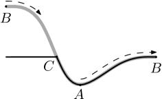
Figure 1: Simple model with singular LDF. The gray curve is $U\left(x\right)=-f_{0}x-V\left(x\right)$, and black curve is the LDF $\phi\left(x\right)$. The dashed arrows show the most probable path for a particle from A, the local minimum of the potential, to a point between B and C. $\phi^{\prime}\left(x\right)$ is discontinuous at point C.

As the noise is small (because of the $\varepsilon$ prefactor), the system spends most of its time near point A. We now want to evaluate the probability $P\left(x\right)\sim e^{-\varepsilon^{-1}\phi\left(x\right)}$ of reaching any other point, in the low noise limit to leading order in $\varepsilon^{-1}$. The point B is represented both by $x=0$ and $x=1$. However, due to the bias force it is easier to reach B by moving to the right. Therefore the probability of reaching point B is given by the Arrenius factor

$$P\sim e^{-\varepsilon^{-1}\left[U\left(1\right)-U\left(A\right)\right]}=e^{-\varepsilon^{-1}\phi\left(B\right)}\ .$$

To see why $\phi\left(x\right)$ is singular, note that once the particle has reached this point it may “roll-down” to reach all points. Therefore the probability of being between B and C is equal to this order. Only below C is it preferable to move from point A to the left, and the probability changes again. Thus for $f_{0}\neq 0$ one obtains a plateau and a discontinuity in $\phi^{\prime}\left(x\right)$ at point C.

While the plateau is a rather specific feature of this and similar examples, the existence of a discontinuity in the derivative $\phi^{\prime}\left(x\right)$ is a common feature of non-equilibrium low-noise systems. It results from a competition between different trajectories which lead to the same final point. Here, these are trajectories moving to the right and left.

In the context of boundary-driven diffusive systems, the LDFs of all models which were previously studied exhibited a smooth LDF. This raises the question of whether, and for what models of this family, will LDSs exist. In addition, it is interesting to understand the structure of these singularities, and whether they are similar to what is known for models in a finite-dimensional space, where the structure can be understood using mean-field, or catastrophe theory.

II.1 Background theory

We now outline the theoretical tools used below. The average, or most probable density profile for the system, $\bar{\rho}$, is obtained by solving $\partial_{x}\left[D\left(\bar{\rho}\right)\partial_{x}\bar{\rho}\right]=0$, with $\bar{\rho}\left(0\right)=\rho_{L}$ and $\bar{\rho}\left(1\right)=\rho_{R}$ at the boundaries. As the noise is small, the system spends most of its time close to $\bar{\rho}$. In order to find the probability of any profile $\rho_{f}\left(x\right)$, one must therefore compute the probability of reaching $\rho_{f}$, starting from $\bar{\rho}$ in the distant past.

The probability density of a history $\left\{\rho\left(x,t\right),J\left(x,t\right)\right\}$ during time $-\infty\leq t\leq 0$ is $P\sim e^{-NS}$ where the action $S$ is given by BertiniPRL ; BertiniJstat ; JSP_quantum ; TKL_long ; Freidlin_Wentzell

$$S=\int_{-\infty}^{0}dt\int_{0}^{1}dx\frac{\left[J\left(x,t\right)+D\left(\rho\left(x,t\right)\right)\partial_{x}\rho\left(x,t\right)\right]^{2}}{2\sigma\left(\rho\left(x,t\right)\right)}\ .$$ (3)

The probability density $P\left[\rho_{f}\right]$ of reaching $\rho_{f}$ is then given by the path integral

$$P\left[\rho_{f}\right]=\int D\rho\int DJe^{-NS\left[\rho,J\right]}\ ,$$

taken over histories satisfying $\partial_{t}\rho+\partial_{x}J=0$, with initial and final conditions $\rho\left(x,t\rightarrow-\infty\right)=\bar{\rho}\left(x\right)$, $\rho\left(x,t=0\right)=\rho_{f}\left(x\right)$, and boundary conditions $\rho\left(x=0,t\right)=\rho_{L}$ and $\rho\left(x=1,t\right)=\rho_{R}$. For large $N$ a saddle-point approximation gives $P\sim e^{-N\phi\left[\rho_{f}\right]}$ with $\phi\left[\rho_{f}\right]=\inf_{\rho,J}S$, where the infimum is over all allowed histories.

In equilibrium (i.e. when $\rho_{L}$ $=\rho_{R}$), the steady-state probability of a density profile $\rho_{f}\left(x\right)$ is easy to obtain – the LDF $\phi\left[\rho_{f}\right]$ is then given by the free-energy which is local in $\rho_{f}$, $\phi[\rho_{f}]=\int f\left(\rho_{f}\left(x\right),\bar{\rho}\right)dx$, where

$$f\left(\rho,r\right)\equiv\int_{r}^{\rho}d\rho_{1}\int_{r}^{\rho_{1}}d\rho_{2}\frac{2D\left(\rho_{2}\right)}{\sigma\left(\rho_{2}\right)}\ .$$ (4)

Note that in this case $\bar{\rho}$ is constant, $\bar{\rho}=\rho_{L}$ $=\rho_{R}$. By contrast, the steady-state probability distribution away from equilibrium is notoriously hard to compute, and very different from the naive guess $\phi[\rho_{f}]=\int f\left(\rho_{f}\left(x\right),\bar{\rho}\left(x\right)\right)dx$, now with space dependent $\bar{\rho}\left(x\right)$. In fact, as stated above, $\phi[\rho_{f}]$ is non-local.

III Existence of LDS

As is clear from Eq. (4), LDSs cannot exist in equilibrium if $D\left(\rho\right)$ and $\sigma\left(\rho\right)$ are smooth, positive functions. We now turn to discuss non-equilibrium cases where they can exist. In previously studied exactly solvable non-equilibrium models SSEP_large_dev ; KMP_large_dev , the action $S$ in Eq. (3) has a single local minimal history leading to $\rho_{f}$, and $\phi\left[\rho_{f}\right]$ is then a smooth functional. However, this need not always be the case, and there can be multiple local minima to $S$ to the same $\rho_{f}$. For example, in the model of a single particle described in Sec. II, these are trajectories corresponding to the particle moving left or right on the ring. When this occurs, the global minimum can switch between the different local minima (as it does at point C in Fig. 1). For fields, this is accompanied by a jump in the functional derivative of the large-deviation $\delta\phi/\delta\rho_{f}$. This is reminiscent of the mechanism for a first-order phase transition in equilibrium.

It is unclear which models display an LDS. It is known that models which feature more than one fixed point of the zero-noise dynamics generically display LDSs Graham_Tel . In the models we study here, however, $\bar{\rho}$ is the only zero-noise fixed-point. Therefore, the absence of LDSs in previously studies models of this class is not surprising SSEP_large_dev ; KMP_large_dev .

In this section we discuss the existence of LDSs in two models. One of the models originates by taking the continuum limit of a “microscopic” lattice gas model, the driven Ising model. The other has the advantage of being exactly solvable. As explained in Sec. II.1, a model is defined by two functions, the diffusivity $D\left(\rho\right)$ and the noise strength $\sigma\left(\rho\right)$. These are shown in Fig. 2(a) for a specific set of parameters of the driven Ising model, and 2(b) for the analytically solvable model, referred to as the quadratic-$\sigma$ (QS) model. We first define the models, and then discuss their properties.

III.1 Definition of models

Here we define two models for which we demonstrate the existence of LDSs. As a common feature, both models display a pronounced dip in the function $\sigma\left(\rho\right)/D\left(\rho\right)$.

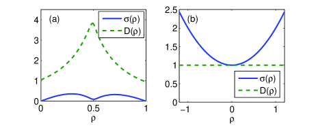
Figure 2: Model definitions. The functions $\sigma\left(\rho\right)$ and $D\left(\rho\right)$ for (a) the BDI model, and (b) the QS model.

III.1.1 The boundary-driven Ising (BDI) model

This is a lattice gas with on-site exclusion and nearest-neighbor interaction. It corresponds to the Katz-Lebowitz-Spohn model KLS with zero bulk bias. The model is defined on a 1d lattice with sites $i=1,..,N$, each of which can be either occupied (“1”) or empty (“0”). The model depends on two rate parameters $\delta$ and $\varepsilon$. The jump rate from site $i$ to site $i+1$ depends on the occupation at sites $i-1$ to $i+2$ according to the following rules:

$$0100\overset{1+\delta}{\rightarrow}0010,\ 1101\overset{1-\delta}{\rightarrow}1011\ ,$$

$$1100\overset{1+\varepsilon}{\rightarrow}1010,\ 1010\overset{1-\varepsilon}{\rightarrow}1100\ ,$$

and their spatially inverted counterparts with identical rates.

For equilibrium BCs, e.g., periodic BCs, the dynamics admits an Ising probability distribution $P\propto\exp\left(-\beta E\right)$ with

$$E=\sum_{i}\left(1-2n_{i}\right)\left(1-2n_{i+1}\right)+\mu\sum_{i}\left(1-2n_{i}\right)\ .$$

This energy describes nearest neighbor interactions, and a chemical potential term. $\beta$ is related to $\varepsilon$ by $\exp\left(4\beta\right)=\left(1+\varepsilon\right)/\left(1-\varepsilon\right)$, and $\mu$ fixes the average density. The parameter $\delta$ does not affect the stationary state, but does enter into the dynamical behavior of the model. For each parameter set $\left(\varepsilon,\delta\right)$ one can write implicit analytic equations for $D\left(\rho\right),\sigma\left(\rho\right)$ which can then be inverted numerically. The calculation is described in Appendix A. Fig. 2(a) shows $D\left(\rho\right)$ and $\sigma\left(\rho\right)$ for $\left(\varepsilon,\delta\right)=\left(0.05,0.995\right)$. As can be seen, $D\left(\rho\right)$ is peaked and $\sigma\left(\rho\right)$ has a local minimum around $\rho=1/2$. This will be a key feature of the model.

III.1.2 The quadratric-$\sigma$ (QS) model

The model is defined by constant $D$ and $\sigma\left(\rho\right)=c\left(\rho-b\right)^{2}+a$, with $a,c>0$, so that $\sigma\left(\rho\right)$ is a parabola clear above the axis. Upon the rescaling

$$\rho \rightarrow\sqrt{\frac{a}{c}}\rho+b\ ,\ J\rightarrow D\sqrt{\frac{a}{c}}J~{},\$$

$$x \rightarrow x\ ,\ t\rightarrow t/D\ ,\ S\rightarrow cS/D$$

the model can be brought to a standard form defined by $D=1$ and $\sigma\left(\rho\right)=\rho^{2}+1$, see Fig. 2(b). This standard form will be used throughout the text. Note that the BCs of the density map accordingly.

The QS model has the advantage that it is analytically tractable KMP_large_dev : the LDF is given by $\phi\left[\rho_{f}\right]=\min\phi_{ext}$, where $\phi_{ext}$ are extremal values of the action given by

$$\phi_{ext}=\int_{0}^{1}dx\left\{f\left(\rho_{f}\left(x\right),g\left(x\right)\right)-\ln\frac{g^{\prime}\left(x\right)}{\bar{\rho}^{\prime}\left(x\right)}\right\}\ .$$ (5)

Here $f\left(\rho,g\right)$ is defined in Eq. (4) and $g\left(x\right)$ is an auxiliary function satisfying the differential equation

$$0=\frac{g\left(x\right)-\rho_{f}\left(x\right)}{\sigma\left(g\left(x\right)\right)}-\frac{g^{\prime\prime}\left(x\right)}{\left[g^{\prime}\left(x\right)\right]^{2}}\ ,$$ (6)

with BCs $g\left(0\right)=\rho_{L}$, and $g\left(1\right)=\rho_{R}$. Note that as $D=1$, the most probable configuration $\bar{\rho}\left(x\right)$ is linear, with $\bar{\rho}\left(0\right)=\rho_{L}$ and $\bar{\rho}\left(1\right)=\rho_{R}$. Each of the solutions of Eq. (6), when used in Eq. (5), gives $\phi_{ext}$ of an extremal path foot_extremize_S .

III.2 The use of cross-sections

Below we demonstrate the existence of LDSs in the models defined above. As the phase-space is infinite dimensional, the structure of $\phi$ is hard to visualize. For many purposes it is sufficient to consider two-dimensional cross-sections of the infinite-dimensional phase-space.

To this end, in most of what follows, out of the phase-space of final profiles $\rho_{f}\left(x\right)$ we restrict ourselves to those parametrized by just two variables, of the form

$$\rho_{f}\left(x\right)=\bar{\rho}\left(x\right)+\alpha_{1}\sin\pi x+\alpha_{2}\sin 2\pi x\ .$$ (7)

This is a cross-section in the phase-space of final states. (Note that in Appendix B we use a different form.) It will be more convenient to parametrize these profiles using $\rho_{f}\left(1/3\right)$ and $\rho_{f}\left(2/3\right)$ instead of $\alpha_{1},\alpha_{2}$. We stress that this choice is rather arbitrary and that the singularity described occupies a space of co-dimension 1 in the infinite-dimensional phase space.

In order to visualize trajectories $\rho\left(x,t\right)$ leading to $\rho_{f}\left(x\right)$, we plot $\rho\left(x=2/3,t\right)$ against $\rho\left(x=1/3,t\right)$. Note that here we do not constrain $\rho\left(x,t\right)$ at intermediate times to be of the form in Eq. (7).

III.3 Non-unique path minimizers and the LDS

As we now show, in both the BDI and the QS models, there are certain states $\rho_{f}$ for which there exists more than a single history $\rho\left(x,t\right)$ that extremalizes the action in Eq. (3). In order to find multiple extremal solutions we use different techniques, depending on the model.

In the QS model we look for solutions to the differential equation (6). These are found using a shooting method numerical_recepies , in which Eq. (6) is integrated from $x=0$ to $x=1$, with initial conditions $g\left(0\right)=\rho_{L}$, and $g^{\prime}\left(0\right)=c$. The values of $c$ are scanned systematically to find all solutions where $g\left(1\right)=\rho_{R}$. In this way all solutions of Eq. (6) are obtained.

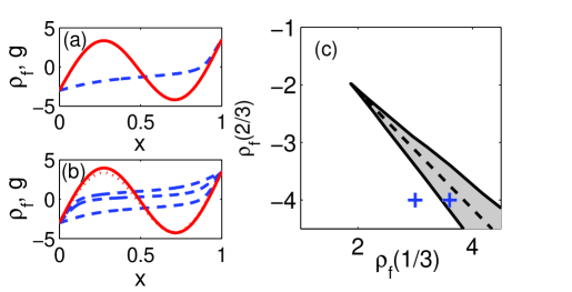
Figure 3: QS cusp. (a) A profile $\rho_{f}$ (solid line) for which Eq. (6) has a single solution (dashed line). (b) A profile $\rho_{f}$ for which Eq. (6) has three solutions. $\rho_{f}$ of panel (a) is shown for comparison (dotted line). (c) A cross-section - the density $\rho_{f}\left(x=2/3\right)$ vs. $\rho_{f}\left(x=2/3\right)$, for configurations of the form given by Eq. (7). The region of multiple solutions (gray), and the switching line (dashed line). Crosses denote the locations in this cross section of the profiles shown in panels (a,b).

Using final profiles $\rho_{f}$ of the form of Eq. (7) with $\rho_{L}=-3,\rho_{R}=3$, we find two distinct behaviors. For final profiles which lie in the white region of Fig. 3(c) we obtain a single solution to Eq. (6), as illustrated in Fig. 3(a). In contrast, for final profiles in the gray region Fig. 3(c) we find three solutions, see Fig. 3(b). Of these three solutions, two correspond to local minima of the action Eq. (3) and one to a saddle-point. Among the two minima, one is lower than the other except along the switching line, marked by a dashed line in Fig. 3(c), where they are equal. On this line the global minimum switches from one local minimum to the other. This leads to a jump in the gradient of the LDF $\delta\phi/\delta\rho_{f}$ across the line.

The phase diagram, shown in Fig. 3(c), is reminiscent of that obtained from a Landau free-energy. In this analogy, the gray region corresponds to the free-energy having two local minima, one metastable. The boundaries of the gray region are then the spinodal lines (where the metastable minimum disappears), and the switching line corresponds to a first-order transition (where the metastable and stable minima exchange roles). The switching line terminates at a point analogous to a critical point. We examine this issue in detail below, and show that a universal behavior emerges.

It is natural to ask which BCs admit profiles $\rho_{f}\left(x\right)$ with multiple minimizing solutions. In the case of the QS model, we can in fact show that: For any BCs $\rho_{L}\neq\rho_{R}$, there exists a profile $\rho_{f}\left(x\right)$ for which Eq. (6) is satisfied by more than one solution. The proof is given in Appendix B. This is interesting since it implies that in this model even the smallest deviation of the BCs from equilibrium leads to the existence of LDSs. The closer the BCs are to equilibrium, the further the states $\rho_{f}$ are from $\bar{\rho}$ before multiple solutions exist.

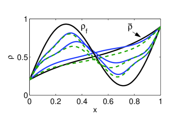
Figure 4: LDS in the BDI model. Two locally minimizing histories leading to the same $\rho_{f}$, plotted at different times.

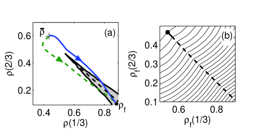
Figure 5: LDS in the BDI model. (a) The time evolution of $\rho\left(1/3,t\right)$ vs. $\rho\left(2/3,t\right)$ is plotted for the histories of Fig. 4. (b) The switching line (dashed line), together with lines of equal $\phi$ (solid lines).

We now turn to the BDI model. Here no analytical solution is known, and we solve for local minimizers of the action $S$, using the numerical technique described in our_numerics ; ours_short . Again, for $\rho_{L}\neq\rho_{R}$ we find final configurations $\rho_{f}$ with multiple minimizing solutions. Fig. 4 gives an example of such a $\rho_{f}$. The two paths leading to this configuration are also shown in Fig. 5(a), where we plot the values of $\rho\left(x=2/3,t\right)$ against $\rho\left(x=1/3,t\right)$ of the same histories. In Fig. 5(a) we also plot the numerically obtained region in the $\rho_{f}\left(1/3\right)$ and $\rho_{f}\left(2/3\right)$ plane for which multiple histories are found, as well as the switching line. The jump in the gradient $\delta\phi/\delta\rho_{f}$ is clear in Fig. 3(b), which depicts lines of equal $\phi$.

The LDSs in the two models have many features in common. The phase diagrams in Fig. 3(c) and 5(a) have a similar structure, with the singularities appearing for similar final profiles $\rho_{f}$. There is one important difference: In contrast to the QS model, in the BDI model a finite difference of the boundary conditions $\rho_{R}-\rho_{L}$ is needed in order for an LDS to exist. In both models, generally we find (data not shown) that as the value $\rho_{R}-\rho_{L}$ is decreased, the region with multiple solutions is pushed away from $\bar{\rho}$. However, in contrast to the QS model where $\rho$ is unbounded, in the BDI model $\rho$ is bounded ($0\leq\rho\leq 1$). Hence below some threshold value, no LDS is found in the BDI model. Similarly, by tuning $\varepsilon$ and $\delta$ in the BDI model, $D$ and $\sigma$ can be continuously varied from the simple symmetric exclusion model with $D=1$ and $\sigma=2\rho\left(1-\rho\right)$, for which the LDF $\phi$ is known to be smooth, to the model discussed above. The singularity appears when the dip in $\sigma\left(\rho\right)/D\left(\rho\right)$ is deep enough (data not shown).

To summarize, in both models we find LDSs when the function $\sigma\left(\rho\right)/D\left(\rho\right)$ has a (deep enough) local minimum. Numerical experiments indicate that this is indeed, more generally, the requirement. Recall that by fluctuation-dissipation, the ratio is related to the compressibility $\sigma\left(\rho\right)/D\left(\rho\right)=2k_{B}T\rho^{2}\kappa\left(\rho\right)$. The profiles where the LDS is found always have a shape similar to that in Fig. 3(b) and Fig. 4. Intuitively, the existence of multiple locally-minimizing histories leading to the same $\rho_{f}$ is due to the favorable action due to large $\sigma\left(\rho\right)$ on certain trajectories, utilizing densities on either side of the minimum in $\sigma\left(\rho\right)$. A similar argument can be given for the ratio $\sigma\left(\rho\right)/D\left(\rho\right)$. The existence and exact location of the LDS depends on the full functional form of $\sigma\left(\rho\right)$ and  $D\left(\rho\right)$. It would be of interest to find precise criteria.

IV Structure of cusp

As discussed above, the structure of the LDS is similar in different models. Consider $\rho_{f}$ in some fixed 2d cross-section of the full phase-space, e.g., the cross-section defined in Eq. (7). As can be seen in Fig. 5(b), the switching line ends at a single profile (a point in the cross-section), which we denote by $\rho_{f}^{cusp}\left(x\right)$. This is much like a first-order transition line ending at a second order point. We now discuss the behavior of the LDF $\phi\left[\rho_{f}\right]$ near $\rho_{f}^{cusp}$, as a function of $\rho_{f}$ and $N$. As we now show, in the simplest scenario $\phi$ behaves like in a Landau mean-field second order phase transition, or a “cusp catastrophe” in the language of catastrophe theory Berry ; catastrophe_ref .

The discussion builds on previous results pertaining to systems with few degrees of freedom Noise_non_lin_book ; MaierSteinCuspBiforcates ; Maier_Stein ; Dykman_cusp_structure ; Dykman . The singularity structure is well understood in such systems, where catastrophe theory is applicable. The extension to fields requires care, as we show below, see discussion at the end of this section. We first present the theoretical considerations. Appendices C and D verify the prediction for the QS and BDI models.

IV.1 Multiple minima near the cusp

The action $S\left[\rho,J\right]$ is a functional of both $\rho$ and $J$. The dependence of $S$ on the current $J$ is quadratic, and at fixed $\rho$ the minimum over $J$, subject to Eq. (1), is unique. It will therefore be convenient to work with the action after $J$ has been minimized:

$$s\left[\rho\right]=\min_{J}S\left[\rho,J\right]\ .$$

Figure 6: Definition of quantities near the cusp. Dashed line - switching line.

For a given $\rho_{f}$ on the switching line there are two histories, $\rho_{1}\left(x,t\right)$ and $\rho_{2}\left(x,t\right)$, which minimize the action, as in Fig. 4. We introduce

$$a=\left[\int\left(\rho_{f}-\rho_{f}^{cusp}\right)^{2}dx\right]^{1/2}$$

as the distance of the final configuration $\rho_{f}$ from $\rho_{f}^{cusp}$, see Fig. 6. We define a coordinate system, $\left(a,b\right)$ on the cross-section, with $\rho_{f}^{cusp}$ at the origin, $\hat{a}$ directed along the switching line and positive on the switching line, and $\hat{b}$ orthogonal to the switching line. In analogy with Landau mean-field theory, $a$ plays the role of $\left(T_{c}-T\right)$ and $b$ the role of the magnetic field.

Close to the cusp, when moving in the positive $a$ direction, for small enough $\left|b\right|$,$\ s$ has two locally-minimizing solutions, $\rho_{1}$ and $\rho_{2}$. Let (see Fig. 6)

$$\rho_{{}_{\left(a,b\right)}}^{avg}\left(x,t\right) =\frac{1}{2}\left[\rho_{1}\left(x,t\right)+\rho_{2}\left(x,t\right)\right]\ ,$$

$$\delta\rho_{\left(a,b\right)}\left(x,t\right) =\frac{1}{2}\left[\rho_{2}\left(x,t\right)-\rho_{1}\left(x,t\right)\right]\ ,$$

$$u_{\left(a,b\right)}\left(x,t\right) =\delta\rho_{\left(a,b\right)}/\left\|\delta\rho_{\left(a,b\right)}\right\|\ .$$ (8)

and

$$\Delta=\left\|\delta\rho\right\|\ ,$$

where we quantify the distance between two histories by $\left\|\delta\rho\right\|^{2}=\int\left[\delta\rho\left(x,t\right)\right]^{2}dxdt$. Here $\Delta$ plays the role of the amplitude of the order parameter. Note that at the cusp $\Delta=0$.

On the switching line $b=0$ and $s\left[\rho_{1}\right]=s\left[\rho_{2}\right]$ by definition. Hence

$$s_{\left(a,b\right)}\left(q\right)=s\left[\rho_{\left(a,b\right)}^{avg}+qu_{\left(a,b\right)}\right]$$

has two minima, at $q_{\min}=\pm\Delta$. $q$ is an “order parameter” interpolating between $\rho_{1}$ and $\rho_{2}$. Close to $\rho_{f}^{cusp}$ the two minima should approach each other, and merge to a single minimum at $\rho_{f}^{cusp}$. The simplest form which captures this behavior and is analytical in $q,a$ and $b$ is

$$\tilde{s}_{\left(a,b\right)}\left(q\right)=s_{\left(a,b\right)}\left(q\right)-s_{\left(a,b\right)}\left(0\right)=c_{4}q^{4}-ac_{2}q^{2}+c_{1}bq\ ,$$ (9)

with $c_{1},c_{2},c_{4}>0$ constants. $\tilde{s}$ can also include higher powers of $q$, which would not affect the behavior at small $a$. At small $a$ and $b=0$, $\tilde{s}\left(q\right)$ has two minima, at $q_{\min}\propto\pm\sqrt{a}$, hence $\Delta\propto\sqrt{a}$ in direct analogy with Landau theory, with a mean-field exponent equal to 1/2.

In Appendix D we check the validity of Eq. (9) on the BDI model. We show that it indeed holds, but that higher order terms are still significant until close to the cusp point ($\left\|\rho_{f}-\rho_{f}^{cusp}\right\|\sim 10^{-2}$). For the QS model we use a different approach, see below.

IV.2 Effect of “soft modes”

When $\rho_{f}$ approaches $\rho_{f}^{cusp}$ from the positive $a$ direction, the height of the action barrier separating the two local minima vanishes. This means that the contribution of the paths close to the minimal paths is enhanced. As we now show, this gives a new universal contribution to the probability of $\rho_{f}^{cusp}$, scaling logarithmically in $N$

$$P\left[\rho_{f}^{cusp}\right]\sim\exp\left(-N\phi\left[\rho_{f}^{cusp}\right]+\frac{1}{4}\log N\right)\ .$$ (10)

The universal factor $1/4$ is known as the Berry index in catastrophe theory Berry .

To see this, we go back to the path integral formulation, $P\left[\rho_{f}\right]=\int D\rho DJ\exp\left\{-NS\left[r,J\right]\right\}$. In this expression, if the path integral is discretized then the measure is $Dx=\prod_{i}\left(\sqrt{N}dx_{i}\right)$, where the $\sqrt{N}$ ensure normalization. For given $\rho\left(x,t\right)$, $S$ is a quadratic functional in $J$, so $J$ can be integrated out. For large $N$ a saddle-point approximation gives

$$\ln\left(\int DJ\exp\left\{-NS\left[\rho,J\right]\right\}\right)=-N\min_{J}S\left[\rho,J\right]=-Ns\left[\rho\right]\ ,$$

and the path integral now reads

$$P\left[\rho_{f}\right]=\int D\rho\left(x,t\right)\exp\left\{-Ns\left[\rho\right]\right\}\ .$$ (11)

Note that the correction to the saddle-point is $N^{0}$ in this case foot_J_min .

We focus on final configurations in the cross-section. Since close to the cusp, when moving in the positive $a$ direction, $s\left[\rho_{f}\right]\,$ has two solutions, this means that the Hessian matrix

$$H\equiv\frac{\delta^{2}s}{\delta\rho_{\left(x_{1},t_{1}\right)}\delta\rho_{\left(x_{2},t_{2}\right)}}$$ (12)

has at least one vanishing eigenvalue for the optimal path ending at $\rho_{f}^{cusp}$. (This is a standard result in catastrophe theory catastrophe_ref .) The corresponding eigenvector $u\left(x,t\right)$ is precisely $u_{\left(a,b\right)}$ defined in Eq. (8) for $\rho_{f}\rightarrow\rho_{f}^{cusp}$, i.e. $u\left(x,t\right)=u_{\left(a\rightarrow 0^{+},b=0\right)}$. As $s$ is minimal, $H$ is positive semi-definite, and its entire spectrum is non-negative. We now assume that there is a single zero eigenvalue, followed by a finite gap. We then split the histories as follows

$$\rho\left(x,t\right)=\rho_{avg}\left(x,t;a,b\right)+qu\left(x,t\right)+\rho_{\perp}\left(x,t;\rho_{f}\left(a,b\right)\right)\ .$$

Here $\rho_{avg}$ is defined as above when there are two minima, and is equal to the minimal history when it is unique. $q$ is a numerical prefactor, and all other contributions are included in $\rho_{\perp}\left(x,t\right)$. Integrating out the $\rho_{\perp}$ directions we are left with an integral over $q$

$$P\left[\rho_{f}\left(a,b\right)\right]\sim e^{-Ns_{\left(a,b\right)}\left(0\right)}N^{1/2}\int dq\exp\left\{-N\tilde{s}_{\left(a,b\right)}\left(q\right)\right\}\ .$$

where $\tilde{s}_{\left(a,b\right)}\left(q\right)$ is defined in Eq. (9). The $N^{1/2}$ comes from the definition of the path integral measure. The form in Eq. (9) was argued on the basis of the analyticity of $\tilde{s}\,$, justified by our assumption of the gap in $H$. The integral

$$\psi\left(N,a,b\right)=N^{1/2}\int dq\exp\left[-N\left(c_{1}bq-c_{2}aq^{2}+c_{4}q^{4}\right)\right]$$

is known as the “cusp diffraction catastrophe” Berry . We note two of its properties: (a) the “metastability” region, where the integrand has two local minima as a function of $q$ is bounded by $b\propto\pm a^{2/3}$. (b) $\psi\left(N,z_{1},z_{2}\right)$ has the scaling property (with $u=N^{1/4}q$)

$$\psi_{N}\left(a,b\right) =N^{1/2}\int dq\exp\left[-N\left(c_{1}bq-c_{2}aq^{2}+c_{4}q^{4}\right)\right]$$

$$=N^{1/4}\Psi\left(N^{1/2}a,N^{3/4}b\right)\ ,$$ (13)

where $\Psi\left(\alpha,\beta\right)=\int dv\exp\left[-\left(c_{1}\beta v-c_{2}\alpha v^{2}+c_{4}v^{4}\right)\right]$ has no $N$ dependence. At $\left(a,b\right)=\left(0,0\right)$ this becomes $\psi\left(0,0\right)=N^{1/4}\Psi\left(0,0\right)$.

Therefore, at $\rho_{f}^{cusp}$ we have $\phi\left[\rho_{f}^{cusp}\right]=s_{\left(a,b\right)}\left(0\right)$, and $P\left[\rho_{f}^{cusp}\right]$ has an additional $N^{1/4}$ prefactor to the probability distribution shown in Eq. (10). This means that at the cusp the exponentiated $N$ dependence has an additional non-analytic contribution, scaling as $\log N$ with a universal prefactor. The exponents $1/4,1/2,3/4$ in Eq. (13) were introduced in arnold and Berry . This implies that the $\log N$ correction in Eq. (10) affects the probability in an elongated region of dimensions $\Delta a\times\Delta b\sim N^{-1/2}\times N^{-3/4}$ around $\rho_{f}^{cusp}$.

The above analysis relies on the assumption that the Hessian spectrum has a single zero mode followed by a gap. This can be generalized to situations where there is a finite number of zero modes followed by a gap, using tools from catastrophe theory. In such cases, more complicated singular structures will appear at $\rho_{f}^{cusp}$, with modified universal exponents. The existence of a gap is expected to always hold in systems with finite-dimensional phase spaces. However, in the case of fields, where the phase space is infinite dimensional, the Hessian may be gapless. Then the analyticity of the action might fail altogether, as indeed happens in equilibrium critical phenomena schulman .

In Appendices C and D we show that the assumptions indeed hold. Specifically, for the QS model, we prove that for specific types of profiles the assumption of analyticity is justified. In addition, we calculate the Hessian spectrum numerically, and find a gap above a single zero mode. For the BDI model, we show numerically that the action indeed has a Landau mean-field form, Eq. (9).

V The connection with finite-dimensional phenomena – a toy model

In an attempt to better understand the LDS in this system, we note that the minimizing histories $\rho\left(x,t\right)$ in Fig. 4 appear to be quite smooth in $x$; this is sensible, as the field is constantly diffusing, making enduring, sharp spatial gradients improbable. This was studied in our_numerics . The smoothness motivates us to introduce toy models with a finite number of degrees of freedom, which capture many of the essential features of the field models described above.

To this end we discretize the field $\rho\,\left(x,t\right)$, replacing it with a vector $\rho_{i}\left(t\right)$, $i=1,..,N_{p}$, corresponding to the density at the points $x_{i}$. Substituting Eq. (2) into Eq. (1), the Langevin equation reads $\partial_{t}\rho=\mathbf{\nabla}\cdot\left[D\left(\rho\right)\mathbf{\nabla}\rho+\sqrt{\sigma\left(\rho\right)}\eta\right]$. For $x\in\left[0,1\right]$, we take $x_{i}=i/(N_{p}+1)$, and obtain $N_{p}$ coupled Langevin equations

$$\partial_{t}\rho_{i} =\left(\Delta x\right)^{-2}\left[D_{i+1/2}\left(\rho_{i+1}-\rho_{i}\right)-D_{i-1/2}\left(\rho_{i}-\rho_{i-1}\right)\right]$$

$$+\left(\Delta x\right)^{-1}\left[\sqrt{\sigma_{i,i+1}}\eta_{i+1/2}-\sqrt{\sigma_{i-1,i}}\eta_{i-1/2}\right]\ ,$$ (14)

where $\Delta x=(N_{p}+1)^{-1}$, and $\rho_{0},\rho_{N_{p}+1}$ are assigned the boundary values $\rho_{B}\left(0\right),\rho_{B}\left(1\right)$ respectively, and $\left\langle\eta_{i+1/2}\eta_{j+1/2}\right\rangle=\left(\Delta x\right)N^{-1}\delta_{i,j}$. $D_{i,i+1},\sigma_{i,i+1}$ are an appropriate choice for $D\left(\rho\right),\sigma\left(\rho\right)$ for $x$ between $x_{i}$ and $x_{i+1}$. We choose $D_{i,i+1}=\frac{1}{2}\left[D\left(\rho_{i}\right)+D\left(\rho_{i+1}\right)\right]$. A similar choice can be made for $\sigma_{i,i+1}$, but we use $\sigma_{i,i+1}=2D_{i,i+1}\left(\rho_{i+1}-\rho_{i}\right)\left[f^{\prime}\left(\rho_{i+1}\right)-f^{\prime}\left(\rho_{i}\right)\right]^{-1}$, where $f^{\prime}\left(\rho\right)$ is given in Eq. (4). This has the advantage that when the BCs are equal, $\rho_{0}=\rho_{N_{p}+1}$, the system of Langevin equations satisfies detailed-balance gardiner with respect to the potential $\phi\left(\left\{\rho_{i}\right\}\right)=\Delta x\sum_{i}f\left(\rho_{i}\right)$. The discrete Langevin equation converges at high $N_{p}$ to the field-theory (as can be seen by writing the action). As the histories are smooth we expect rapid convergence for long wave lengths. We therefore use the lowest non-trivial discretization, $N_{p}=2$, which can accommodate non-equilibrium phenomena. In this case $\rho_{1,2}$ correspond to “coarse-grained” densities at $x=1/3,2/3$ respectively.

The minimizing histories for the toy model with $N_{p}=2$ can be obtained using standard techniques from low-noise finite-dimensional systems. Using the approach outlined in the introduction, a set of coupled ordinary differential equation is obtained, whose solutions are the extremizing histories. The equations are solved numerically using a shooting methodGraham_Tel .

In Fig. 7 we check the above approach on the simple symmetric exclusion model (SSEP) with $D=1$ and $\sigma=2\rho\left(1-\rho\right)$, which does not feature a cusp, and for the BDI model. We plot trajectories of the toy version of the SSEP (Fig. 7(a)) and the BDI model (Fig. 7(b)) in the $\left(\rho_{1},\rho_{2}\right)$ plane, against the $\left(\rho_{1/3},\rho_{2/3}\right)$ trajectories of the full models. In addition, the metastability region for the toy model and in the cross-section of the exact dynamics are plotted. The qualitative picture is similar – a metastability region appears in the quadrant $\rho_{1/3}>0,\rho_{2/3}<0$, at approximately the same location as in the exact field solution. This is expected to have a close relation to the breaking of detailed-balance, which is easy to visualize in the two-dimensional toy model. Define the two-variable Langevin equation $dx_{i}/dt=K_{i}\left(x_{1},x_{2}\right)+\sum_{j=1,2}B_{ij}\eta_{j}$, and let $\mathbf{Q}\equiv\mathbf{BB}^{T}$. Detailed-balance is satisfied if $\mathbf{\nabla}\phi=\mathbf{Q}^{-1}\mathbf{K}$, or $\nabla\times\left(\mathbf{Q}^{-1}\mathbf{K}\right)=0$. Therefore, in two (phase-space) dimensions $\omega=\nabla\times\left(\mathbf{Q}^{-1}\mathbf{K}\right)$ is a scalar which quantifies the breaking of detailed balance. It is shown in Fig. 8. Minimizing trajectories passing through regions with $\omega>0$ ($\omega<0$) bend counter-clockwise (clockwise). Therefore, a gradient in $\omega$ can cause trajectories to focus and cross, creating a cusp. A similar picture has been discussed for other finite-dimensional systems Dykman .

In summary, the above analysis shows that much of the phenomena observed can be captured by simplified finite-dimensional models, making concrete connections to previous works on such models.

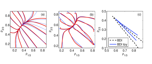
Figure 7: (a) Toy model paths (thin lines) compared with cross-sections of exact paths for the SSEP model. (b) Same as (a) for BDI model. (c) Cusp area for toy vs. exact in the BDI model. BCs are $\rho_{L}=0.2,\rho_{R}=0.9$.

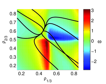
Figure 8: Map of $\omega$, the measure for breaking of detailed-balance, in the BDI model. Clockwise currents for positive $\omega$. In black: selected baths.

VI Discussion

Many interesting questions remain to be studied. First, it would be of interest to find precise conditions or bounds for the occurrence of the LDSs, depending on the boundary conditions and model parameters. In addition, a simple picture for the mechanism leading to the existence of multiple histories ending at the same final profile is lacking. The mechanism suggested by the current authors in ours_short was flawed foot_sleeve_flaw .

The singularity described above has the simplest possible structure. More complicated singularities are in principle possible. For instance, in catastrophe theory, richer structures have been analyzed. Observing them in full requires one to look at higher dimensional cross-sections. It would be interesting to find which of them exist in diffusive models, and for which models. Even more exciting possibilities exist: Fields allow for the possibility that the Hessian discussed in Sec. IV is gapless. Thus, it may even be possible to find singularities that are beyond the realm of catastrophe theory.

Finally, it would be very interesting to look at these LDSs in higher dimensional systems. This is now possible using the numerical technique described in our_numerics , and used in the present paper.

Acknowledgments - We are grateful for discussions with B. Derrida, J. Kurchan, O. Raz and J. Tailleur. This research was funded by the BSF, ISF, and IRG grants.

Appendix A Calculating $D\left(\rho\right)$ and $\sigma\left(\rho\right)$ for the driven Ising model

As shown in spohn_book ; KLS_sigma , for each parameter set $\left(\varepsilon,\delta\right)$ one can write implicit analytic equations for $D\left(\rho\right)$ which can then be inverted numerically. Then $\sigma\left(\rho\right)$ is obtained via the fluctuation-dissipation relation, $\sigma\left(\rho\right)=2k_{B}T\rho^{2}\kappa\left(\rho\right)D\left(\rho\right)$ where $\kappa\left(\rho\right)$ is the compressibility Derrida_review . For equilibrium BCs this model admits an Ising measure.

To find $D\left(\rho\right)$, we use the relation foot_gradient_cond

$$D=\frac{1}{2\chi}\left(\left\langle j_{i,i+1}\right\rangle+\left\langle j_{i,i-1}\right\rangle\right)=\frac{1}{\chi}\left\langle j_{i,i+1}\right\rangle$$

where $\chi=\sum_{i}\left(\left\langle n_{i}n_{0}\right\rangle-\rho^{2}\right)$ (related to the compressibility $\kappa\left(\rho\right)$ by $\chi=k_{B}T\rho^{2}\kappa\left(\rho\right)$), $j_{i,i+1}$ is the current (number of particles per unit time) from site $i$ to site $i+1$. The averages are taken with respect to the equilibrium probability distribution, and $\left\langle j_{i,i+1}\right\rangle=\left\langle j_{i,i-1}\right\rangle$ due to the symmetries in equilibrium. One then finds $\sigma$ using

$$\sigma=2\chi D=2\left\langle j_{i,i+1}\right\rangle\ .$$

To calculate $\left\langle j_{i,i+1}\right\rangle$ note that as the rates depend on the four sites around a bond, we have that

$$\left\langle j_{i,i+1}\right\rangle =\left(1+\delta\right)P_{0100}+\left(1+\varepsilon\right)P_{1100}$$

$$+\left(1-\varepsilon\right)P_{0101}+\left(1-\delta\right)P_{1101}$$

where $P_{0100}$ is the probability of the pattern $0100$, and similarly for others. Using the transfer-matrix technique KLS_sigma , one can calculate these probabilities and obtain

$$\left\langle j_{i,i+1}\right\rangle=\frac{\lambda\left[1+\delta\left(1-2\rho\right)\right]-\varepsilon\sqrt{4\rho\left(1-\rho\right)}}{\lambda^{3}}$$

where

$$\lambda=\frac{1}{\sqrt{4\rho\left(1-\rho\right)}}+\left(\frac{1}{4\rho\left(1-\rho\right)}-1+\frac{1-\varepsilon}{1+\varepsilon}\right)^{1/2}\ .$$

It remains to find $\rho$ and $\kappa$, which are both given in terms of $\beta$ (recall that $\exp\left(4\beta\right)=\left(1+\varepsilon\right)/\left(1-\varepsilon\right)$), and $h=\beta\mu$:

$$\rho =\frac{1}{2}\left(1+\frac{\sinh h}{\sqrt{e^{4\beta}+\sinh^{2}h}}\right)~{},$$

$$\chi =\frac{e^{4\beta}\cosh h}{4\left(e^{4\beta}+\sinh^{2}h\right)^{3/2}}\ .$$

In order to obtain $D\left(\rho\right),\sigma\left(\rho\right)$, we calculate $\sigma\left(h\right),D\left(h\right)$ and $\rho\left(h\right)$ for a wide range of $h$, and numerically invert the last to find $D\left(\rho\right)=D\left(h\left(\rho\right)\right)$ and $\sigma\left(\rho\right)=\sigma\left(h\left(\rho\right)\right)$. Fig. 2(a) shows $D\left(\rho\right)$ and $\sigma\left(\rho\right)$ for $\left(\varepsilon,\delta\right)=\left(0.05,0.995\right)$.

As a check, we note that for the simple symmetric exclusion process Derrida_review $\delta=\varepsilon=0$, and one finds

$$\rho=\frac{1}{2}\left(1+\tanh h\right)\ ;\ \ \chi=\frac{1}{4\cosh^{2}h}=\rho\left(1-\rho\right)$$

and

$$\lambda=2\cosh h\ ;\ \ \ \left\langle j_{i,i+1}\right\rangle=\lambda^{-2}=\frac{1}{4\cosh^{2}h}$$

so that $D=1$ and $\sigma=2\rho\left(1-\rho\right)$ Derrida_review .

Appendix B Existence of multiple extremal solutions in the QS model

In this Appendix we prove that for the QS model, which has $D=1$ and $\sigma\left(\rho\right)=\rho^{2}+1$, and for any non-equilibrium BCs, there exists a LDS for some profiles. Here it will be far more convenient to work in the domain $x\in\left[-1,1\right]$. The results in the new domain are simply related to the results in the original domain foot_QS_change_vars .

The BCs to Eq. (6) are denoted by $\rho_{-1}\equiv\rho_{L}$ and $\rho_{+1}\equiv\rho_{R}$.

Claim 1

For any BCs $\rho_{-1}\neq\rho_{+1}$, there exists a profile $\rho_{f}\left(x\right)$ for which Eq. (6) is satisfied by more than one solution with $g\left(\pm 1\right)=\rho_{\pm 1}$.

Proof. Using the symmetries $\rho\rightarrow-\rho$ and $x\rightarrow-x$ it is enough to consider the case $\rho_{-1}<\rho_{1}$, and $0<\rho_{1}$.

We proceed by an explicit construction of $\rho_{f}$. That is, given $\rho_{\pm 1}$ we construct a function $\rho_{f}\left(x\right)$ for which Eq. (6) is satisfied by more than one function $g\left(x\right)$, which also satisfies the boundary-conditions. The profile $\rho_{f}\left(x\right)$ will be a piecewise-constant function composed of two flat regions, of the form

$$\rho_{f}\left(x\right)=\left\{\begin{array}[c]{ccc}\rho_{A}&&-1<x<0\\ \rho_{B}&&0<x<1\end{array}\right.\ ,$$ (15)

where $\rho_{A},\rho_{B}$ are (constant) numbers which specify $\rho_{f}\left(x\right)$, see Fig. 9. Note that $\rho_{f}\left(x\right)$ does not have to be continuous, nor to satisfy the BCs, hence $\rho_{A},\rho_{B}$ are not restricted in any way. The solutions $g\left(x\right)$ will be put together by solving Eq. (6) for $x<0$ and $x>0$ separately (each with its corresponding boundary condition), and matching the solutions by demanding that $g\left(x\right)$ and $g^{\prime}\left(x\right)$ are continuous at $x=0$.

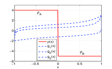
Figure 9: Density profile $\rho\left(x\right)$ of the step form (Eq. (15)), and three $g\left(x\right)$ solutions. Here $\rho_{A}=4,\rho_{B}=-5,\rho_{-1}=-2,\rho_{1}=3$.

For a region with constant $\rho\left(x\right)=\bar{\rho}$, and given $g\left(x_{1}\right)$, Eq. (6) has an (implicit) analytic solution

$$\int_{g\left(x_{1}\right)}^{g\left(x\right)}\frac{e^{\bar{\rho}\operatorname{atan}\psi}}{\sqrt{1+\psi^{2}}}d\psi=c_{1}\left(x-x_{1}\right)\ ,$$ (16)

where $c_{1}$ is a free constant. Differentiating both sides with respect to $x$ we find

$$g^{\prime}\left(x\right)\frac{e^{\bar{\rho}\operatorname{atan}g\left(x\right)}}{\sqrt{1+g\left(x\right)^{2}}}=c_{1}$$ (17)

and using Eq. (16) for $c_{1}$, $g^{\prime}\left(x\right)$ reads

$$g^{\prime}\left(x\right)=\frac{\sqrt{1+g\left(x\right)^{2}}}{e^{\bar{\rho}\operatorname{atan}\phi\left(x\right)}}\frac{1}{x-x_{1}}\int_{g\left(x_{1}\right)}^{g\left(x\right)}\frac{e^{\bar{\rho}\operatorname{atan}\psi}}{\sqrt{1+\psi^{2}}}d\psi\ .$$ (18)

Note that $c_{1}$ no longer appears in this equation. Instead, this is a relation between $g\left(x\right)$ and $g^{\prime}\left(x\right)$. Let $g_{A}\left(x\right)$ be the solution given in Eq. (16) with $x_{1}=-1$, $g\left(x_{1}\right)=\rho_{-1}$ and $\bar{\rho}=\rho_{A}$:

$$\int_{\rho_{-1}}^{g_{A}\left(x\right)}\frac{e^{\rho_{A}\operatorname{atan}\psi}}{\sqrt{1+\psi^{2}}}d\psi=c_{A}\left(x+1\right)\ ,$$ (19)

for $-1<x<0$. This defines a one-parameter family of solutions, according to the value of $c_{A}$. Similarly, $g_{B}\left(x\right)$ is defined by

$$\int_{\rho_{1}}^{g_{B}\left(x\right)}\frac{e^{\rho_{B}\operatorname{atan}\psi}}{\sqrt{1+\psi^{2}}}d\psi=c_{B}\left(x-1\right)$$ (20)

for $0<x<1$. Any solution of Eq. (6) with $\rho\left(x\right)$ of the step form defined in Eq. (15) is composed of solutions $g_{A}\left(x\right),g_{B}\left(x\right)$ satisfying $g_{A}\left(0\right)=g_{B}\left(0\right)$ and $g_{A}^{\prime}\left(0\right)=g_{B}^{\prime}\left(0\right)$. The derivatives at $x=0$ are given by

$$g_{A}^{\prime}\left(0\right) =\frac{\sqrt{1+g_{A}\left(0\right)^{2}}}{e^{\rho_{A}\operatorname{atan}g_{A}\left(0\right)}}\int_{\rho_{-1}}^{g_{A}\left(0\right)}\frac{e^{\rho_{A}\operatorname{atan}\psi}}{\sqrt{1+\psi^{2}}}d\psi\ ,$$

$$g_{B}^{\prime}\left(0\right) =\frac{\sqrt{1+g_{B}\left(0\right)^{2}}}{e^{\rho_{B}\operatorname{atan}g_{A}\left(0\right)}}\int_{g_{B}\left(0\right)}^{\rho_{1}}\frac{e^{\rho_{B}\operatorname{atan}\psi}}{\sqrt{1+\psi^{2}}}d\psi\ .$$ (21)

We note that:

1. $g^{\prime}\left(x\right)$ does not change sign. As we are interested in solutions with $\rho_{-1}<\rho_{1}$, we only need to consider solutions with $g^{\prime}\left(x\right)\geq 0$.

2. From (a) it follows that $\rho_{-1}\leq g_{A}\left(0\right)=g_{B}\left(0\right)\leq\rho_{1}$.

3. It also follows that if $g_{A}\left(0\right)=\rho_{-1}$ then $g_{A}^{\prime}\left(0\right)=0$, and if $g_{B}\left(0\right)=\rho_{1}$ then $g_{B}^{\prime}\left(0\right)=0$. Similarly, if $g_{A}\left(0\right)=\rho_{1}$ then $g_{A}^{\prime}\left(0\right)>0$, and if $g_{B}\left(0\right)=\rho_{-1}$ then $g_{B}^{\prime}\left(0\right)>0$.

Consider now $g_{A}^{\prime}\left(0\right)$ and $g_{B}^{\prime}\left(0\right)$ as a function of $g\left(0\right)$. A solution $g\left(x\right)~{}$on the entire segment $\left[-1,1\right]$ is obtained when $g_{A}^{\prime}\left(0\right)=g_{B}^{\prime}\left(0\right)$ for the same $g\left(0\right)$. Remark (c) ensures that they cross at least once; But they may also cross more than once, see Fig. 10. The number of crossings depends on $\rho_{A},\rho_{B}$. We will show that there always exist $\rho_{A},\rho_{B}$ for which the graphs cross more than once.

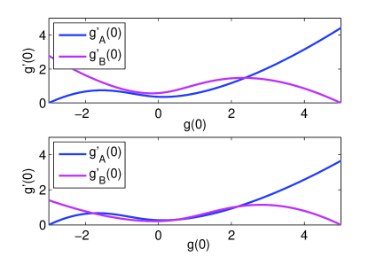
Figure 10: $g_{A}^{\prime}\left(0\right)$ and $g_{B}^{\prime}\left(0\right)$ plotted as functions of $g\left(0\right)$ for two functions $\rho\left(x\right)$. In the upper pane the graphs cross only once, indicating a single $g\left(x\right)$-solution. In the lower pane, done with parameters of Fig. (9), they cross three times, resulting in three different $g$-solutions. (Note that the $g$-values at these crossings indeed correspond to $g\left(0\right)$ of the solutions in Fig. (9)). BCs for both panels are $\rho_{-1}=-3,\rho_{+1}=5$. Upper panel: $\rho_{A}=3,\rho_{B}$ $=-2$, lower panel: $\rho_{A}=4,\rho_{B}$ $=-5$.

Motivated by the fact that the cusp singularities always appear at the lower right corner of our phase-space cross-sections, we consider the limit where $\rho_{A}$ is a large positive number, and $\rho_{B}\simeq-\rho_{A}$.

Denote by $g_{A}^{\prime}\left[g\left(0\right);\rho_{A};\rho_{-1}\right]$ the value of $g_{A}^{\prime}\left(0\right)$ as a function of $g\left(0\right),\rho_{A}$ and $\rho_{-1}$ , and similarly $g_{B}^{\prime}\left[g\left(0\right);\rho_{B};\rho_{1}\right]$. The analysis which follows is done for $g_{A}^{\prime}\left(0\right)$; similar results are obtained for $g_{B}^{\prime}\left(0\right)$ since $g_{B}^{\prime}\left[g\left(0\right);\rho_{B};\rho_{1}\right]=g_{A}^{\prime}\left[-g\left(0\right);-\rho_{B};-\rho_{1}\right]$. To better understand $g_{A}^{\prime}\left[g\left(0\right);\rho_{A};\rho_{-1}\right]$ at large $\rho_{A}$, we plot $g_{A}^{\prime}\left[g\left(0\right)\right]$ for $\rho_{A}=100$ and different $\rho_{-1}$ values, see Fig. 11. As can be seen, the different graphs rise quickly from $g_{A}^{\prime}\left(0\right)=0$ at $g\left(0\right)=\rho_{-1}$, and join a common function.

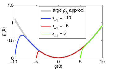
Figure 11: $g_{A}^{\prime}\left[g\left(0\right);\rho_{A}=100;\rho_{-1}\right]$ for different $\rho_{-1}$. Gray line: large $\rho$-expansion, Eq. (22).

This is formulated by the following Lemma:

Lemma 2

Expanding around $\rho_{A}\rightarrow\infty$, we have for any $g\left(0\right)>\rho_{-1}$

$$g_{A}^{\prime}\left[g;\rho_{A};\rho_{-1}\right]=\frac{1+g^{2}}{\rho_{A}}-\frac{g\left(1+g^{2}\right)}{\rho_{A}^{2}}+O\left(\rho_{A}^{-3}\right)\ \text{.}$$ (22)

Proof. Rewrite Eq. (21) for $g_{A}^{\prime}\left(0\right)$ as

$$g_{A}^{\prime}\left(0\right)=\sqrt{1+g^{2}}\int_{\rho_{-1}}^{g}\frac{e^{-\rho_{A}\left[\operatorname{atan}g-\operatorname{atan}\psi\right]}}{\sqrt{1+\psi^{2}}}d\psi\ ,$$

where here and in the next equation $g$ stands for $g_{A}\left(0\right)$. For $\rho_{A}\rightarrow\infty$ a saddle-point approximation can be preformed. The exponent $-\rho_{A}\left[\operatorname{atan}\phi-\operatorname{atan}\psi\right]$ is dominated by small values of $g-\psi$, i.e. close to the upper bound of the integral, and $\operatorname{atan}\phi-\operatorname{atan}\psi$ can be expanded to second order

$$\operatorname{atan}g-\operatorname{atan}\psi=\frac{g-\psi}{1+g^{2}}+g\frac{\left(g-\psi\right)^{2}}{\left(1+g^{2}\right)^{2}}+O\left(\left(g-\psi\right)^{3}\right)\ .$$

In addition, the denominator $\left(1+\psi^{2}\right)^{-1/2}$ is expanded to second order around $g$. The resulting expression involves Gaussian integrals which can be integrated, with the lower integration limit set to $-\infty$. Finally, we expand the result (containing error-functions, etc.) to second order in $1/\rho_{A}$ around $\rho_{A}\rightarrow\infty$, and obtain Eq. (22).   

The expression in Eq. (22) does not depend on $\rho_{-1}$, as expected from the reasoning alluding to Fig. 11. Similarly, for $g_{B}^{\prime}\left[g\left(0\right);\rho_{B};\rho_{1}\right]$ we have, for $\rho_{B}\rightarrow-\infty$,

$$g_{B}^{\prime}\left[g;\rho_{B};\rho_{1}\right]=-\frac{1+g^{2}}{\rho_{B}}+\frac{g\left(1+g^{2}\right)}{\rho_{B}^{2}}+O\left(\rho_{B}^{-3}\right)\ \text{.}$$ (23)

We are now in a position to construct $\rho_{f}\left(x\right)$ with three solution to $g$: given the BCs, choose some crossing value $g_{c}\in\left(\rho_{-1},\rho_{1}\right)$ (this is where the non-equilibrium condition $\rho_{-1}\neq\rho_{1}$ enters). For a given $\rho_{A}$ the condition $g_{A}^{\prime}\left[g_{c};\rho_{A};\rho_{-1}\right]=g_{B}^{\prime}\left[g_{c};\rho_{B};\rho_{1}\right]$, together with Eqs. (22),(23) reads, to second order in $\rho_{A}^{-1},\rho_{B}^{-1}$,

$$\frac{1+g_{c}^{2}}{\rho_{A}}-\frac{g_{c}\left(1+g_{c}^{2}\right)}{\rho_{A}^{2}}=-\frac{1+g_{c}^{2}}{\rho_{B}}+\frac{g_{c}\left(1+g_{c}^{2}\right)}{\rho_{B}^{2}}\ ,$$ (24)

or

$$\frac{1}{\rho_{A}}\left(1-\frac{g_{c}}{\rho_{A}}\right)=-\frac{1}{\rho_{B}}\left(1-\frac{g_{c}}{\rho_{B}}\right)\ .$$ (25)

Solving this for $\rho_{B}$ we find

$$\rho_{B}=\frac{-1-\sqrt{1+4\frac{g_{c}}{\rho_{A}}\left(1-\frac{g_{c}}{\rho_{A}}\right)}}{2\left(1-\frac{g_{c}}{\rho_{A}}\right)}\ .$$ (26)

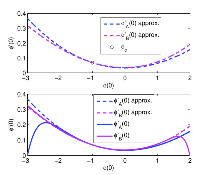
Figure 12: Constructing a solution. Choose a crossing value $g_{c}$ (here $g_{c}=-1$) and some large $\rho_{A}$. $\rho_{B}$ is fixed so that the crossing is approximately at $g_{c}$ (Upper pane). The full solutions will feature this crossing with two more crossings, close to the boundaries.

Fixing $g_{c}$, the expansions Eqs. (22),(23) guarantee that as $\rho_{A}$ grows, with $\rho_{B}$ given by Eq. (26), a crossing point will appear in a neighborhood of $g_{c}$, and approach $g_{c}$ for $\rho_{A}\rightarrow\infty$. The root of the quadratic equation leading to Eq. (26) was chosen so that $g_{A}^{\prime},g_{B}^{\prime}$ will cross from $g_{A}^{\prime}\left[g\right]>g_{B}^{\prime}\left[g\right]$ for $g<g_{c}$, to $g_{A}^{\prime}\left[g\right]<g_{B}^{\prime}\left[g\right]$ for $g>g_{c}$, see Fig. 12. This, together with $g_{A}^{\prime}\left[\rho_{-1};\rho_{A};\rho_{-1}\right]=0$ and $g_{B}^{\prime}\left[\rho_{1};\rho_{B};\rho_{1}\right]=0$, guarantees that the functions $g_{A}^{\prime}\left[g;\rho_{A};\rho_{-1}\right]$ and $g_{B}^{\prime}\left[g;\rho_{B};\rho_{1}\right]$, will have two crossing points in addition to the crossing point near $g=g_{c}$. For large $\rho_{A}$ these will be at values of $g$ close to $\rho_{-1}$ and $\rho_{+1}$, see Fig. (12).   

Appendix C Cusp Structure and Hessian spectrum in the QS model

In this appendix we study the cusp structure, and the spectrum of the Hessian matrix $H$ at $\rho_{f}^{cusp}$, for the QS model. First, we prove that for the QS model with profiles defined as in Appendix B, the framework of catastrophe theory is applicable. More precisely, there exists an analytical function $F\left(\rho_{A},\rho_{B}\right)$ on the two-dimensional cross-section parametrized by $\left(\rho_{A},\rho_{B}\right)$ as in Appendix B, and for which every extremum of $F$ corresponds to a single extremal history leading to $\rho_{f}\left(\rho_{A},\rho_{B}\right)$, as defined in Eq. (15).

To construct the function $F$, we note that Eqs. (21) give us analytical expressions $g_{A}^{\prime}\left(0\right)=f_{A}\left(g_{0},\rho_{A},\rho_{B}\right)$ and $g_{B}^{\prime}\left(0\right)=f_{B}\left(g_{0},\rho_{A},\rho_{B}\right)$. We drop the $\rho_{-1},\rho_{1}$ dependence, which are kept fixed. Let

$$F\left(g_{0};\rho_{A},\rho_{B}\right)\equiv\left[g_{A}^{\prime}\left(0\right)-g_{B}^{\prime}\left(0\right)\right]^{2}\ .$$

$F\left(\phi_{0};\rho_{A},\rho_{B}\right)$ is analytic in all its variables, and $F\left(g_{0};\rho_{A},\rho_{B}\right)=0$ iff the solution $g$ is an extremal solution. Moreover, in the vicinity of the cusp, $\partial F/\partial g_{0}=0$ iff $F\left(g_{0};\rho_{A},\rho_{B}\right)=0$, i.e. is a local minimum as a function of $g_{0}$. Therefore $F$ acts as a “gradient map” (in the sense of Catastrophe Theory), with $\rho_{A},\rho_{B}$ the control variables, and $g_{0}$ the state variable. Accordingly, the cusp structure (regions in $\left(\rho_{A},\rho_{B}\right)$ where $F\left(g_{0}\right)=0$ has two solutions) is expected to be mean-field.

To show how $F$ is used, we briefly review the argument for the cusp structure, which is essentially a Landau mean-field argument. The cusp point is a special point $\left(\rho_{A}^{cusp},\rho_{B}^{cusp}\right)$ where at the minimal $g_{0}$, $\partial^{2}F/\partial g_{0}^{2}=0=\partial^{3}F/\partial g_{0}^{3}$ hold (the two conditions explain why it is a point, or a set of isolated points, in the $\left(\rho_{A},\rho_{B}\right)$ plane). Let $x_{A,B}=\rho_{A,B}-\rho_{A}^{cusp}$. In the vicinity of the cusp, expand $F$ to forth-order (here the analyticity is crucial), $F=\alpha g_{0}^{4}+\beta g_{0}^{3}+\gamma g_{0}^{2}+\delta$, where $\alpha,\beta,\gamma,\delta$ depend on $x_{A,B}$. We assume that $\alpha\neq 0$; vanishing $\alpha$ would be non-generic, i.e., could be remedied by a small change in any additional parameters, such as the BCs $\rho_{-1},\rho_{1}$ or the noise function $\sigma$. Then a local change of variables can be performed to bring $F$ to the form $F=\frac{1}{4}g_{0}^{4}+ag_{0}^{2}+b$, where at the cusp $a=0=b$. The region where $F$ has two local minima is bounded by $b=\pm\frac{2}{3^{3/2}}a^{3/2}$. Near the cusp $a,b$ can be expanded to first order in $x_{A,B}$, so the power-law relation between $b\propto\pm a^{3/2}$ will apply to a rotated frame of $x_{A,B}$.

C.1 Spectrum

As discussed in the main text, for the “Landau mean-field”, catastrophe theory to hold, one must have a gap in the spectrum of the Hessian $H$. This can be tested numerically, by evaluating the action $S$ for the extremal solution $\rho\left(x,t\right)$ leading to $\rho_{f}\left(x\right)$, and calculating the Hessian, Eq. (12), by varying $\rho$ jointly at pairs of points $\left(x_{1},t_{1}\right)\$and $\left(x_{2},t_{2}\right)$. The eigenvalues of $H$ can then be calculated for different $\rho_{f}$ profiles close to $\rho_{f}=\rho_{cusp}$.

To calculate $H$ one thus needs to locate $\rho_{cusp}$. This is most easily done for the QS model with BCs $\rho_{L}=-\rho_{R}$, where $\rho_{cusp}$ of the form of Eq. (7) must have $\alpha_{1}=0$. Fig. 13 shows the bottom of the spectra of $H$ for different $\rho_{f}$, starting from $\bar{\rho}$ and ending at $\rho_{cusp}$. One can clearly see a single eigenvalue going to zero, in agreement with the analysis in the paper. The rest of the eigenvalues remain away from zero, without closing the gap. This validates the analysis carried out in the main text for the QS model.

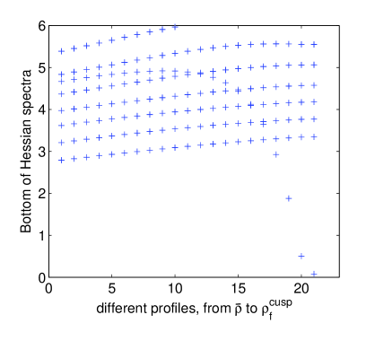
Figure 13: Bottom of Hessian spectrum for the QS model at different $\rho_{f}$ profiles, equaly spaced between $\bar{\rho}$ (leftmost) to $\rho_{f}^{cusp}$ (rightmost). BCs are $\rho_{L}=-3,\rho_{R}=3$. A single eigenvalue approaches zero, while the gap above it is maintained.

Appendix D Cusp structure in the BDI model

In this Appendix we check the validity of Eq. (9), which predicts the structure of the cusp. In the BDI model the diagonalization of the Hessian $H$ gave inconclusive results. We suspect that this is due to the difficulty of locating $\rho_{cusp}$ with high precision in this model. As we show now, the predictions of Sec. IV hold only very close to $\rho_{f}^{cusp}$, when $\left\|\rho_{f}-\rho_{f}^{cusp}\right\|<10^{-2}$.

To compare Eq. (9) with numerics, it is more convenient to use a different form, which does not require knowing the precise position of $\rho_{f}^{cusp}$. Noting that $s_{\left(a,0\right)}\left(\Delta\right)=s\left[\rho_{1}\right]$ and $s_{\left(a,0\right)}\left(-\Delta\right)=s\left[\rho_{2}\right]$, we find that $\Delta\propto\sqrt{a}$. Therefore we expect that for $b=0$

$$s_{q}\left(\Delta\right)-s_{q=0}\left(\Delta\right)\propto\Delta^{4}\left(\frac{1}{4}y^{4}+\frac{1}{2}y^{2}\right)\ ,$$ (27)

where $y=q/\Delta$.

As an example we consider the boundary-driven Ising model, with $\left(\varepsilon,\delta\right)=\left(0.05,0.995\right)$ and $\rho_{L}=0.2,\rho_{R}=0.8$. Examples of pairs of locally minimizing histories leading to configurations on the switching line are shown in Fig. 14.

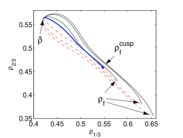
Figure 14: Pairs of locally minimizing histories, leading to points on the switching line (solid and dashed lines). The history leading to $\rho_{f}^{cusp}$ (circle) is also plotted (bold line).

Fig. 15(a) shows the function $\left[s_{q}\left(\Delta\right)-s_{q=0}\left(\Delta\right)\right]/\Delta^{4}$ as a function of $y$ at $a\sim 10^{-2}$, together with a quartic fit, which shows clear deviations from this form. This means that even at this distance $\rho_{f}-\rho_{f}^{cusp}\sim 10^{-2}$ there are significant contributions of higher powers to $S_{q}$. Due to these higher powers plotting $\left[s_{q}\left(\Delta\right)-s_{q=0}\left(\Delta\right)\right]/\Delta^{4}$ vs. $y$ for different $a$ values in the range $5\cdot 10^{-3}\leq a\leq 0.2$ does not collapse the data as expected. We therefore fit the functions $s_{q}\left(\Delta\right)-s_{q=0}\left(\Delta\right)$ to polynomials of order four and higher, and plot $c_{4}$, the prefactor of $q^{4}$, as a function of $\Delta^{2}$, see Fig. 15(b). The expected power-law is not obtained for a quartic fit, but improves when the fits include higher order terms, see Fig. 16(a). This means that $c_{4}$ in Eq. (9) can indeed be taken to be constant. Finally, one can also fit $s_{q}\left(\Delta\right)-s_{q=0}\left(\Delta\right)\propto a^{2}\left(\frac{1}{4}y^{4}+\frac{c}{2}y^{2}\right)$, by fitting the position of $\rho_{f}^{cusp}$, see Fig. 16(b).

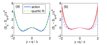
Figure 15: (a) The function $S_{q}\left(\Delta\right)-S_{q=0}\left(\Delta\right)/\Delta^{4}$  as a function of $y$ at $a=0.012$ (solid line). A clear deviation is seen from a fit to a quartic function (dashed line). (b) The function $S_{q}\left(\Delta\right)-S_{q=0}\left(\Delta\right)/\Delta^{4}$ for different values of $a$ (dashed lines). Fitting the functions to a polynomial of power 8, and plotting only the quartic part, the collapse improves significantly (solid lines).

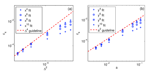
Figure 16: Fits of $c_{4}$. (a) $c_{4}$ as a function of $\Delta^{2}$. (a) $c_{4}$ as a function of $a$. Guidelines (dashed lines) represent the expected slope of the functions. Extracting $c_{4}$ from fits that also include higher powers one obtains data that better fits the expected slope.

The presence of strong higher powers as close as $a\sim 10^{-2}$, see e.g. Fig. 16(b), can be understood as follows: the non-linear terms come from the different action at the two paths $\rho_{1}$ and $\rho_{2}$. As the distance $\Delta$ between the, scales as $\Delta\propto\sqrt{a}$, $\rho_{1}-\rho_{2}$ at some space time point, can be of order $10^{-1}$ even for $a\sim 10^{-2}$, and the two minimizing paths can see very different behavior of $D\left(\rho\right),\sigma\left(\rho\right)$ along the paths. This sensitivity explains why computing $H$ directly is difficult: one needs $\Delta$ to be small, but as $a\propto\Delta^{2}$, one needs the distance $a$ from $\rho_{f}^{cusp}$ to be very small.

From the above we conclude that at the cusp there is a soft mode, a direction along which the minimizing history $\rho^{cusp}\left(x,t\right)$ has a zero second derivative: $d^{2}s\left[\rho^{cusp}\left(x,t\right)+qu_{a=0}\left(x,t\right)\right]/dq^{2}=\left[d^{2}s_{q}/dq^{2}\right]_{a=0}=0$. This is indirect evidence that $H$ has at least one vanishing eigenvalue.

References

- (1) B. Derrida, J. Stat. Mech. P07023 (2007)
- (2) H. Spohn, Large Scale Dynamics of Interacting Particles, Springer Verlag (1991)
- (3) A. N. Jordan, E. V. Sukhorukov, and S. Pilgram, J. Math. Phys. 45 4386-4417 (2004)
- (4) L. Bertini, A. De Sole, D. Gabrielli, G. Jona-Lasinio, and C. Landim, Phys. Rev. Lett. 87, 040601 (2001)
- (5) J. Tailleur, J. Kurchan, and V. Lecomte, J. Phys. A: Math. Theor. 41 505001 (2008)
- (6) W. Dieterich, P. Fulde and I. Peschel, Adv. in Phys. 29 (1980)
- (7) C. Kipnis, C. Marchioro and E. Presutti, J. Stat. Phys. 27 65 (1982)
- (8) J. R. Dorfman, T. R. Kirkpatrick and J. V. Sengers, Annu. Rev. Phys. Chem. 45 213-39 (1994)
- (9) H. Spohn, J. Phys. A: Math. Gen. 16 4275 (1983)
- (10) B. Derrida, J. L. Lebowitz, and E. R. Speer, J. Stat. Phys. 107 (2002)
- (11) L. Bertini, A. De Sole, D. Gabrielli, G. Jona-Lasinio, and C. Landim, J. Stat. Phys. 107 (2002)
- (12) L. Bertini, D. Gabrielli, and J. Lebowitz, J. Stat. Phys. 121 843 (2005)
- (13) G. Bunin, Y. Kafri, and D. Podolsky, EPL 99 (2012) 20002
- (14) R. Graham and T. Tél, Phys. Rev. Lett. 52, 9–12 (1984), R. Graham and T. Tél, J. Stat. Phys., Vol. 35, Nos. 5/6 (1984), R. Graham and T. Tél, Phys. Rev. A Vol. 33, No. 2 (1986), R. Graham and T. Tél, Phys. Rev. A Vol. 31, No. 2 (1985)
- (15) F. Moss and P. V. E. McClintock, ed., Noise in Nonlinear Dynamical Systems, Cambridge University Press, Cambridge (1989)
- (16) D. G. Luchinsky, P. V. E. McClintock, and M. I. Dykman, Rep. Prog. Phys., 61(8):889-997 (1998)
- (17) R. S. Maier and D. L. Stein, Phys. Rev. E, 48(2):931-938 (1993)
- (18) M.I. Dykman, M.M. Millonas and V.N. Smelyanskiy, Phys. Lett. A, 195, 53 (1994)
- (19) M. I. Dykman, D. G. Luchinsky, P. V. E. McClintock, V. N. Smelyanskiy, Phys. Rev. Lett. 77 26 (1996)
- (20) L. Bertini, A. De Sole, D. Gabrielli, G. Jona-Lasinio, and C. Landim, J. Stat. Mech. (2010) L11001
- (21) G. Bunin, Y. Kafri and D. Podolsky, J. Stat. Mech. L10001 (2012)
- (22) L. Bertini, A. De Sole, D. Gabrielli, G. Jona-Lasinio, and C. Landim, Phys. Rev. Lett. 94, 030601 (2005)
- (23) T. Bodineau and B. Derrida, Phys. Rev. E 72, 066110 (2005)
- (24) N. Merhav and Y. Kafri, J. Stat. Mech. P02011 (2010)
- (25) P. I. Hurtado and P. L. Garrido Phys. Rev. Lett. 107, 180601 (2011)
- (26) M. I. Freidlinand A. D. Wentzell, Random Perturbations of Dynamical Systems, Springer-Verlag (1984)
- (27) S. Katz, J. L. Lebowitz, and H. Spohn, J. Stat. Phys., 34, 3/4 (1984)
- (28) The paths which extremize are given by with .
- (29) W. H. Press, S. A. Teukolsky, W. T. Vetterling and B. P. Flannery, Numerical Recipes. The Art of Scientific Computing, 3rd Ed. (2007)
- (30) M.V. Berry, C. Upstill, Progress in Optics, Vol. 18, 257–346 (1980)
- (31) R. Gilmore, “Catastrophe Theory” in digital Encyclopedia of Applied Physics, John Wiley & Sons (2003)
- (32) The action is quadratic in , therefore the minimum of over is unique. The spectrum of is gapped if is bounded away from zero on the path . This justifies the saddle-point approximation (i.e., higher order corrections to this equation are ).
- (33) R. S. Maier and D. L. Stein, Phys. Rev. Lett. 85, 1358 (2000)
- (34) V. I. Arnold, Russian Math. Surveys 30, 1–75 (1975)
- (35) L. S. Schulman and M. Revzen. Collec. Phen., 1: 43-49 (1972)
- (36) Referring to ours_short , the estimate for the LDF of the history which satisfies the symmetry did not take into account the possibility that all the mass transfer occurs at the middle point .
- (37) J. S. Hager, J. Krug, V. Popkov and G. M. Schütz, Phys. Rev. E, 63, 056110 (2001)
- (38) C. W. Gardiner, Handbook of stochastic methods for physics, chemistry, and the natural sciences, Springer (1994)
- (39) This holds for models that satisfy the “Gradient Condition”, see spohn_book .
- (40) Changing variables and , the continuity equation is unchanged and the transformed action Eq. (3) reads . Clearly, the number of extrema of the action for a given is not affected by this change.