Estimation from Relative Measurements in Mobile Networks with Markovian Switching Topology: Clock Skew and Offset Estimation for Time Synchronization

Abstract

We analyze a distributed algorithm for estimation of scalar parameters belonging to nodes in a mobile network from noisy relative measurements. The motivation comes from the problem of clock skew and offset estimation for the purpose of time synchronization. The time variation of the network was modeled as a Markov chain. The estimates are shown to be mean square convergent under fairly weak assumptions on the Markov chain, as long as the union of the graphs is connected. Expressions for the asymptotic mean and correlation are also provided. The Markovian switching topology model of mobile networks is justified for certain node mobility models through empirically estimated conditional entropy measures.

,

1 Introduction

We consider the problem of estimation of variables in a network of mobile nodes in which pairs of communicating nodes can obtain noisy measurement of the difference between the variables associated with them. Specifically, suppose the $u$-th node of a network has an associated node variable $x_{u}\in\mathbb{R}$. If nodes $u$ and $v$ are neighbors at discrete time index $k$, then they can obtain a measurement $\zeta_{u,v}(k)$ where

$$\zeta_{u,v}(k)=x_{u}-x_{v}+\epsilon_{u,v}(k).$$ (1)

The problem is for each node to estimate its node variable from the relative measurements it collects over time, without requiring any centralized information processing or coordination. We assume that at least one node knows its variable. Otherwise the problem is indeterminate up to a constant. A node that knows its node variable is called a reference node. All nodes are allowed to be mobile, so that their neighbors may change with time.

The problem of time synchronization (also called clock-synchronization) through clock skew and offset estimation falls into this category, and provides the main motivation for the study. Time synchronization in ad-hoc networks, especially in wireless sensor networks, has been a topic of intense study in recent years. The utility of data collected and transmitted by sensor nodes depend directly on the accuracy of the time-stamps. In TDMA based communication schemes, accurate time synchronization is required for the sensors to communicate with other sensors. Operation on a pre-scheduled sleep-wake cycle for energy conservation and lifetime maximization also requires accurate knowledge of a common global time. We refer the interested reader to the review papers [1, 2, 3] for more details on time synchronization.

The relationship between local clock time $\tau_{u}(t)$ of node $u$ and global time $t$ is usually modeled as $\tau_{u}(t)=\alpha_{u}t+\beta_{u}$, where the scalars $\alpha_{u},\beta_{u}$ are called its skew and offset, respectively [1, 3]. A node can determine the global time $t$ from its local clock time by using the relationship $\hat{t}=(\tau_{u}(t)-\hat{\beta}_{u})/\hat{\alpha}_{u}$ as long as it can obtain estimates $\hat{\alpha}_{u},\hat{\beta}_{u}$ of the skew and offset of its local clock. Hence the problem is clock synchronization in a network can be alternatively posed as the problem of nodes estimating their skews and offsets. It is not possible for a node to measure its skew and offset directly. However, it is possible for a pair of neighboring nodes to measure the difference between their offsets and logarithm of skews by exchanging a number of time stamped messages. Existing protocols to perform so-called pairwise synchronization, such as [4, 5, 6], can be used to obtain such relative measurements. The details will be described in Section 2.1. The problem of clock offset and skew estimation can therefore be cast as a special case of the estimation from relative measurements described above. If an algorithm is available to solve the scalar node variable estimation problem, nodes can execute two copies of this algorithm in parallel to estimate both skew and offset. Therefore we only consider the scalar case. In the context of time synchronization, the existence of a reference node means that at least one node has access to the global time $t$. This is the case when at least one node is equipped with a GPS receiver, in which case that node has access to the UTC (Coordinated Universal Time). If no node has a GPS receiver, then one node has to be elected to be the reference so that it’s local clock time is considered the global time that everyone has to synchronize to.

1.1 Related work

Time synchronization in sensor networks can be classified into pairwise synchronization and global synchronization methods. In pairwise synchronization, a pair of nodes try to synchronize their clocks to each other. In practice this is often achieved by one of the nodes estimating its relative offset and/or skew with respect to the other node, so that the local time of the other node serves as a reference [4, 5, 6, 7]. Precise definitions of relative offset and relative skew are postponed till Section 2.1. In global synchronization, also called network-wide synchronization, all nodes synchronize themselves to a common time.

A common approach for global synchronization in sensor networks is to first elect a root node and construct a spanning tree of the network with the root node being the “level 0” node. Every node thereafter synchronizes itself to a node of lower level (higher up in the hierarchy) by using a pairwise synchronization method. Examples of such spanning-tree based protocols include Timing-Sync Protocol for Sensor Networks (TPSN) [8] and Flooding Time Synchronization Protocol (FTSP) [9]. Change in the network topology due to node mobility or node failure requires recomputing the spanning tree and sometimes even re-election of the root node. This adds considerable communication overhead. The situation gets worse if nodes move rapidly.

Recently, a number of fully distributed global synchronization algorithms have been proposed that do not need spanning tree computation. Distributed protocols are therefore more readily applicable to mobile networks than tree-based protocols. Among the distributed synchronization protocols proposed, some are based on estimation of the skew and/or offset of each clock with respect to a reference clock (called absolute time synchronization). The algorithms proposed in [10, 11, 12, 13, 14] belong to this category. Another class of protocols estimate a common global time that may not be related to the time of any clock in the network. The algorithms proposed in [15, 16, 17] belong to this category, which we call virtual time synchronization.

1.2 Contribution

In this paper we consider the problem of distributed estimation of skews and offsets with respect to a reference clock in a mobile network for global absolute time synchronization, where the network changes with time due to nodes’ motion. The common thread among virtual time synchronization methods mentioned earlier is the use of consensus-type algorithms to construct virtual skew and offsets that every node agrees to. In many applications, absolute time synchronization is preferable over virtual time synchronization. This occurs when the user of the sensor network is interested in the time of an event that is measured in an absolute reference time, such as UTC provided by a GPS unit on a base station. Therefore, in this paper we consider only absolute time synchronization.

We analyze an algorithm for estimating absolute skews and offsets from noisy pairwise relative measurements of skews and offsets, which is a slight modification of the algorithms proposed in [18, 10, 12]. Though the algorithm is adopted from these earlier papers, the analysis in those papers were limited to static networks. Thus, little is known about how such an algorithm will perform in a mobile network.

The main contribution is that we analyze the convergence of the algorithm when the network topology changes due to the motion of the nodes, as well as random communication failure. We model the resulting time-varying topology of the network as the state of a Markov chain. Techniques for the analysis of jump linear systems from [19] are used to study convergence of the algorithm. We show that under fairly weak assumptions on the Markov chain, the proposed algorithm is mean square convergent if and only if the union of the graphs that occur is connected. Mean square convergence means the expected value and the variance of the estimates obtained by each node converges to fixed values that do not depend on the initial conditions. When the relative measurements are unbiased, then limiting mean is the same as the true value of the variable, meaning the estimates obtained are asymptotically unbiased. Formulas for the limiting mean and variance are obtained by utilizing results from jump linear systems.

The algorithm we analyze bears a close resemblance to consensus algorithms. In fact, the estimation error dynamics turns out to be a leader-follower consensus algorithm, where the leader states - corresponding to the estimation error of the reference nodes - are always $0$. However, existing results from consensus cannot be directly used to analyze the scenario examined in this paper. Consensus literature almost always treats the problem where all nodes participates in the consensus algorithm, i.e., “leaderless consensus”, while ours is a “leader-follower” consensus since the reference nodes error state stays at $0$. One may expect analysis of this case would be easier, but that turns out to be not the case. Even though the literature on consensus is extensive, the topic of consensus with both time-varying graph topology and additive measurement noise is considered only in a limited number of papers, e.g. [20, 21, 22, 23]. There are several differences between the consensus algorithms studied in [20, 21, 22, 23] and the error dynamics examined in this paper, which preclude using their results to perform the analysis. These include requirement of symmetry or balance in graphs/matrices, preassignment of time-varying gains that must be synchronized among all nodes, etc. None of these restrictions are imposed in our analysis (see Remark 4 for more details).

Another contribution of the paper is to provide justification for the Markovian switching topology for mobile networks. The Markovian switching model has also been used extensively in studying consensus protocols in networks with dynamic topologies [24, 25, 26, 21]. For a network of static nodes with link drops, the Markovian switching model arises naturally from Markovian link drop model. In mobile networks, though, the only case where we can prove that a mobile network evolves according to a Markov chain is when nodes move according to the so-called random walk mobility model [27]. Although the Markovian switching assumption facilitates analysis, this assumption requires justification for more complex motion models. We use a technique from [28] to check if the graph switching is Markovian if nodes according to the so-called Random Waypoint Mobility (RWP) model. The RWP model is one of the most widely used mobility models for ad-hoc mobile networks [27]. We show that the resulting graph switching process can indeed be approximated well by a (first order) Markovian switching model.

A preliminary version of this paper was presented in [29]. Compared to that paper, we make several additional contributions. While the paper [29] provided only sufficient conditions for mean square convergence, here we provide both necessary and sufficient conditions. An assumption of symmetry of certain matrices were made in [29], which is removed in the present paper.

The rest of the paper is organized as follows. Section 2 describes the connection between the problem of estimation from relative measurements and the problem of skew/offset estimation, and then states the problem precisely. Section 3 describes the proposed algorithm and states the main result (Theorem 2). It also discusses the relevance of the Markovian switching topology model. Section 4 is devoted to the proof of the theorem. Simulation studies are presented in Section 5.

2 The estimation problem

We consider the problem of estimating the scalar parameters (called node variables) $x_{u}$, $u=1,\dots,n_{b}$, where $n_{b}$ is the number of nodes in the network that do not know their node variables. We assume that there are $n_{r}$ additional nodes that knows their node variables, where $n_{r}\geq 1$. These define a node set ${\mathpzc{V}}=\{1,\dots,n\}$, where $n=n_{b}+n_{r}$ is the total number of nodes. For later reference, we define ${\mathpzc{V}}_{b}:=\{1,\dots,n_{b}\}$ and ${\mathpzc{V}}_{r}=\{n_{b}+1,\dots,n_{b}+n_{r}\}$, so that ${\mathpzc{V}}={\mathpzc{V}}_{b}\cup{\mathpzc{V}}_{r}$. Note that $n=n_{b}+n_{r}$. Time is measured by a discrete time-index $k=0,1,\dots$. The mobile nodes define a time-varying undirected measurement graph $\mathcal{G}(k)=({\mathpzc{V}},{\mathpzc{E}}(k))$, where $(u,v)\in{\mathpzc{E}}(k)$ if and only if $u$ and $v$ can obtain a relative measurement of the form (1) during the time interval between the time indices $k$ and $k+1$. Specifically, for each $(u,v)\in{\mathpzc{E}}(k)$, there is a measurement $\zeta_{u,v}(k)=x_{u}-x_{v}+\epsilon_{u,v}(k)$ that is available to both $u$ and $v$ at time $k$. In practice, one of the two nodes computes this measurement from sensed information. We assume that if $u$ computes the measurement $\zeta_{u,v}$, it then sends this measurement to $v$ so that $v$ also has access to the same measurement. We follow the convention that the relative measurement between $u$ and $v$ that is obtained by the node $u$ is always of $x_{u}-x_{v}$ while that used by $v$ is always of $x_{v}-x_{u}$. Since the same measurement is shared by a pair of neighboring nodes, if $v$ receives the measurement $\zeta_{v,u}$ from $u$, then it converts the measurement to $\zeta_{v,u}$ by assigning $\zeta_{v,u}(k):=-\zeta_{u,v}(k)$. We assume, without any loss of generality, that between a pair of nodes $u$ and $v$, the node with the lower index obtains the relative measurement between them first, and then shares with the node with the higher index.

The neighbors of $u$ at $k$, denoted by $\mathcal{N}_{u}(k)$, is the set of nodes that $u$ has an edge with in the measurement graph $\mathcal{G}(k)$. We assume that if $v\in\mathcal{N}_{u}(k)$, then $u$ and $v$ can also exchange information through wireless communication at time $k$. Therefore, if one prefers to think of a communication graph, we assume that it is the same as the measurement graph.

The task is to estimate the node variables $x_{u}$ for $u=1,\dots,n$ by using the relative measurements $\zeta_{u,v}(k),(u,v)\in{\mathpzc{E}}(k)$ that becomes available over time $k=0,1,\dots$. In addition, the algorithm has to be distributed in the sense that each node has to estimate its own variables, and at every time $k$, a node $u$ can only exchange information with its neighbors $\mathcal{N}_{u}(k)$. Note that the estimation problem is indeterminate unless $n_{r}>0$.

2.1 Relation to skew and offset estimation

To see the connection between skew/offset estimation and the problem of estimation from noisy relative measurements introduced in the previous section, we first discuss the notion of pairwise synchronization between a pair of neighboring nodes $u$ and $v$. By exchanging a number of time-stamped messages, it is possible for node $u$ to estimate the so-called relative skew $\alpha_{u,v}$ and relative offset $\beta_{u,v}$ between itself and $v$, where

$$\tau_{u}(t)=\alpha_{u,v}\tau_{v}(t)+\beta_{u,v}.$$ (2)

That is, the parameters $\alpha_{u,v}$ and $\beta_{u,v}$ relate the local time of $u$ to the local time of $v$ at the same global time $t$. A number of methods are available that allows pairwise synchronization between a node pair from time-stamped messages [4, 5, 30, 13, 6]. The parameters $\alpha_{u,v}$ and $\beta_{u,v}$ are also referred to as the skew and offset of node $u$ with respect to node $v$ [7].

The relationship between the absolute skew and offset $\alpha_{u},\beta_{u},\alpha_{v},\beta_{v}$ and relative skew and offset $\alpha_{u,v},\beta_{u,v}$ is given by

$$\alpha_{u,v} :=\frac{\alpha_{u}}{\alpha_{v}} \beta_{u,v} :=\beta_{u}-\beta_{v}\frac{\alpha_{u}}{\alpha_{v}}.$$ (3)

This relationship is obtained by expressing the local time $\tau_{u}(t)$ of node $u$ at global time $t$ in terms of the local time $\tau_{v}(t)$ at node $v$ at the same time $t$ by using (1):

$$\tau_{u}(t) =\alpha_{u}(\frac{\tau_{v}(t)-\beta_{v}}{\alpha_{v}})+\beta_{u}=\frac{\alpha_{u}}{\alpha_{v}}\tau_{v}(t)+\beta_{u}-\beta_{v}\frac{\alpha_{u}}{\alpha_{v}},$$

and comparing with (2). Suppose a node $u$ obtains noisy estimates $\hat{\alpha}_{u,v},\hat{\beta}_{u,v}$ of the parameters $\alpha_{u,v},\beta_{u,v}$ by using a pairwise synchronization protocol.

1. We model the noisy estimate of $\alpha_{u,v}$ as

   $$\hat{\alpha}_{u,v} =\exp(\epsilon_{u,v}^{s})\alpha_{u,v}$$ (4)

   where $\exp(\cdot)$ is exponential function and $\epsilon_{u,v}^{s}$ is a random variable. If the estimation error is small, then $\epsilon_{u,v}^{s}$ is close to $0$. Taking log, we get

   $$\log\hat{\alpha}_{u,v} =\log\alpha_{u,v}+\epsilon_{u,v}^{s}=\log\alpha_{u}-\log\alpha_{v}+\epsilon_{u,v}^{s}.$$ (5)

   Eq. (5) can be rewritten as $\zeta_{u,v}^{s}=x_{u}^{s}-x_{v}^{s}+\epsilon_{u,v}^{s}$, with the definitions $\zeta_{u,v}^{s}:=\log\hat{\alpha}_{u,v}$ and $x_{i}^{s}:=\log\alpha_{u}$, which makes $\zeta_{u,v}^{s}$ a noisy relative measurement of the node variables $x_{u}^{s}$ and $x_{v}^{s}$; cf. (1). It is important to notice that $\zeta_{u,v}^{s}$ is a measured quantity – since $\hat{\alpha}_{u,v}$ is measured – while the variables $x_{u}^{s},x_{v}^{s}$, which are logarithms of the skews, are unknown.

2. Similarly, the noisy estimate $\hat{\beta}_{u,v}$ of $\beta_{u,v}$ with random estimation error $e_{u,v}^{o}$ can be written as

   $$\hat{\beta}_{u,v} =\beta_{u,v}+e_{u,v}^{o}=\beta_{u}-\beta_{v}+\epsilon_{u,v}^{o},$$ (6)

   where $\epsilon_{u,v}^{o}:=\beta_{v}(1-\alpha_{u}/\alpha_{v})+e^{o}_{u,v}$. Again, (6) can be rewritten as $\zeta_{u,v}^{o}=x_{u}^{o}-x_{v}^{o}+\epsilon_{u,v}^{o}$, with the definitions $\zeta_{u,v}^{o}:=\hat{\beta}_{u,v}$ and $x_{u}^{o}:=\beta_{u}$, which makes $\zeta_{u,v}^{o}$ a noisy relative measurements of the node variables $x_{u}^{o}$ and $x_{v}^{o}$; cf. (1). In this case the node variables are the clock offsets $\beta_{u}$’s. The noise $\epsilon_{u,v}^{o}$ in the offset measurement is in general biased even if the measurement of the relative offset $\beta_{u,v}$ is unbiased.

This discussion shows that the estimates of the relative skew and the relative offset between a pair of neighboring nodes, which can be obtained by existing algorithms for pairwise synchronization, can be expressed as a noisy relative measurement of node variables by appropriate redefinitions. The node variables are log-skews and offsets. Once node $u$ obtains estimates $\hat{x}_{u}^{s}$ and $\hat{x}_{u}^{o}$ of its two node variables $x_{u}^{s}$ and $x_{u}^{o}$, it can estimate its skew and offset as $\hat{\alpha}_{u}:=\exp(\hat{x}_{u}^{s})$ and $\hat{\beta}_{u}:=\hat{x}_{u}^{o}$. Thus, the problem of estimating the skews and offsets of all the clocks in a network can be transformed to an estimation from relative measurements problem, where relative measurements are of the form (1).

Remark 1.

From this point on, we only consider the estimation problem involving scalar node variables. This entails no loss of generality since estimation of the two scalar variables, skew and offset, can be performed in parallel. In the skew estimation problem, log-skews take the role of node variables and $\log\hat{\alpha}_{u,v}$’s obtained from pairwise synchronization take the role of relative measurements. In the offset estimation problem, node variables are the offsets and relative measurements are the $\hat{\beta}_{u,v}$’s obtained from pairwise synchronization. The assumption on the existence of the reference node is equivalent to at least one node knowing the global time. This can be achieved by either one or more nodes having access to GPS time, or by arbitrarily electing a node as a reference and choosing its local time as the global time.

3 Algorithm and results

3.1 Algorithm for distributed estimation from relative measurement

The algorithm we consider is adopted from [10, 12, 18], with minor modification to make it applicable to time varying networks. Each node $u$ maintains in its local memory an estimate $\hat{x}_{u}(k)$ of its node variable $x_{u}\in\mathbb{R}$. Every node - except the reference nodes - iteratively updates its estimate as we’ll describe now. The estimates can be initialized to arbitrary values. In executing the algorithm at iteration $k$, node $u$ communicates with its current neighbors to obtain measurements $\zeta_{u,v}(k)$ and their current estimates $\hat{x}_{v}(k)$, $v\in\mathcal{N}_{u}(k)$. Since obtaining measurements require exchanging time-stamped messages, the current estimates can be easily exchanged during the process of obtaining new measurements. Node $u$ then updates its estimate according to

$$\hat{x}_{u}(k+1)=\left\{\begin{array}[]{rcl}\frac{w_{uu}(k)\hat{x}_{u}(k)+\sum_{v\in\mathcal{N}_{u}(k)}w_{vu}(k)(\hat{x}_{v}(k)+\zeta_{u,v}(k))}{w_{uu}(k)+\sum_{v\in\mathcal{N}_{u}(k)}w_{vu}(k)},&u\in{\mathpzc{V}}_{b}\\ x_{u},&u\in{\mathpzc{V}}_{r},\end{array}\right.$$ (9)

where the weights $w_{vu}(k)$ and $w_{uu}(k)$ are arbitrary positive numbers. The update law is well-defined even at times when $u$ has no neighbors. Nodes continue this iterative update unless they see little change in their local estimates, at which point they can stop updating. The update procedure in each node $u\in{\mathpzc{V}}_{b}$ is specified in Algorithm 1.

Algorithm 1 Distributed update at node $u$

1:Initialize estimate $\hat{x}_{u}(0)\in\mathbb{R}$ and local iteration counter $k=0$

2:while $u$ is performing iteration do

3:     if $\mathcal{N}_{u}(k_{u})\neq\emptyset$ then

4:         for $v\in\mathcal{N}_{u}(k)$ do

5:              if $u$ does not have $\zeta_{u,v}(k)$ then

6:                  1.$u$ and $v$ perform pairwise synchronization: $u$ obtains $\zeta_{u,v}(k)$, $v$ obtains $\zeta_{v,u}(k)$;

7:                  2.$u$ and $v$ exchange their current estimates: $u$ saves $\hat{x}_{v}(k)$; $v$ saves $\hat{x}_{u}(k)$;

8:              else

9:                  $u$ does not communicate with $v$;

10:              end if

11:         end for

12:         $u$ updates $\hat{x}_{u}(k+1)$ using (9);

13:     else

14:         $\hat{x}_{u}(k+1)\leftarrow\hat{x}_{u}(k)$;

15:     end if

16:     $k$=$k+1$;

17:end while

Each node $u$ is allowed to vary its local weights $w_{uv}(k)$ with time and use distinct weights for distinct neighbors to account for the heterogeneity in measurement quality. Between two neighbors $p,q$ of node $u$ at time $k$, the relative measurement $\zeta_{u,p}(k)$ between $u$ and $p$ may have lower measurement error than the relative measurement $\zeta_{u,q}(k)$ between $u$ and $q$. This occurs, for example, if $u$ and $p$ were able to exchange more time stamped messages than $u$ and $q$ before computing the relative measurements [6, 7]. In this case, node $u$ should choose its local weights at $k$ so that $w_{pu}(k)>w_{qu}(k)$. Due to the denominator in (9), it is only the ratios among the weights that matter, not their absolute values.

3.1.1 Asynchronous implementation

The description so far is in terms of a common global iteration index $k$. In practice, nodes do not have access to such a global index. Instead, each node keeps a local iteration index. After every increment of the local index, the node tries to collect a new set of relative measurements with respect to one or more of its neighbors within a pre-specified time interval. At the end of the time interval, whether it is able to get new measurements or not, it updates its estimate according to the update law (9) and increments its local iteration counter. Now the index $k$ in (9) has to be interpreted as the local iteration index. The process then repeats. It follows from (9) that if a node is unable to gather new measurements from any neighbors, then its updated estimate is precisely the previous estimate.

The global iteration index is useful to describe the algorithm from the point of view of an omniscient spectator. Let $T$ the time interval, say, in seconds, between two successive increments of the global index $k$. The parameter $T$ is arbitrary, as long as is small enough so that no node updates its local estimate more than once with the time interval $T$. In that case, one of only two events are possible for an arbitrary node $u$ at the end of the time interval when the global counter is increased from $k$ to $k+1$: (i) $u$ either increases its local index by one, or (ii) $u$ does not increases its local index. If a node increases its local index, both the local and global indices increase by one. A node does not increase its local iteration index if it is not able to gather new measurements. In the omniscient spectator’s view, the node’s neighbor set is empty at this time index; so according to (9), the next estimate of the node’s variable is the same as the previous one. Thus, a node’s local asynchronous state update can be described in terms of the synchronous algorithm (9); the latter being more convenient for exposition. We therefore consider only the synchronous version in the sequel.

3.2 Convergence analysis with Markovian switching

In this paper we model the sequence of measurement graphs $\{\mathcal{G}(k)\}_{k=0}^{\infty}$ that appear as time progresses as the realization of a (first order) Markov chain, whose state space $\mathbb{G}=\{\mathcal{G}_{1},\dots,\mathcal{G}_{N}\}$ is the set of graphs that can occur over time. The Markovian switching assumption on the graphs means that $P(\mathcal{G}(k+1)=\mathcal{G}_{i}|\mathcal{G}(k)=\mathcal{G}_{j})=P(\mathcal{G}(k+1)=\mathcal{G}_{i}|\mathcal{G}(k)=\mathcal{G}_{j},\mathcal{G}(k-1)=\mathcal{G}_{\ell},\dots,\mathcal{G}(0)=\mathcal{G}_{p})$ where $\mathcal{G}_{i},\mathcal{G}_{j},\mathcal{G}_{\ell},\dots,\mathcal{G}_{p}\in\mathbb{G}$ and where $P(\cdot)$ denotes probability. We assume that the Markov chain is homogeneous, and denote the transition probability matrix of the chain by $\mathcal{P}$, in which $p_{ij}$ is the $(i,j)$-th entry of $\mathcal{P}$. Further discussion on Markov modeling of graphs is postponed till Appendix A.

Let $e_{u}(k):=\hat{x}_{u}(k)-x_{u}$ be the estimation error at node $u$. Since $\zeta_{u,v}(k)=x_{u}-x_{v}+\epsilon_{u,v}(k)$, the update law (9) can be rewritten as

$$e_{u}(k+1)=\left\{\begin{array}[]{rcl}\frac{w_{uu}(k)e_{u}(k)+\sum_{v\in\mathcal{N}_{u}(k)}w_{vu}(k)(e_{v}(k)+\epsilon_{u,v}(k))}{w_{uu}(k)+\sum_{v\in\mathcal{N}_{u}(k)}w_{vu}(k)}&\mbox{for}&u\in{\mathpzc{V}}_{b}\\ 0&\mbox{for}&u\in{\mathpzc{V}}_{r},\end{array}\right.$$ (12)

The right hand side of (12) is a weighted average of estimation errors of $x_{u}$ and measurement noise. If the measurement noise $\epsilon_{u,v}(k)$ is zero-mean and the initial estimates are unbiased, i.e. $\operatorname{E}[e_{u}(0)]=0$, $\forall u\in{\mathpzc{V}}_{b}$, then $\operatorname{E}[e_{u}(k)]=0$ for all $k$, where $\operatorname{E}[\cdot]$ denotes expectation.

The main result of the paper - on the mean square convergence of (12) - is stated below as a theorem. In the statement of theorem, $\mathbf{e}(k):=[e_{1}(k),\dots,e_{n_{b}}(k)]^{T}$ is the estimation error vector. Moreover, $\mbox{\boldmath$\mu$}(k):=\operatorname{E}[\mathbf{e}(k)]$ is the mean and $\mathbf{Q}(k):=\operatorname{E}[\mathbf{e}(k){\mathbf{e}(k)}^{T}]$ is the correlation matrix of the estimation error vector. We say that a stochastic process $\mathbf{y}(k)$ is mean square convergent if $\operatorname{E}[\mathbf{y}(k)]$ and $\operatorname{E}[\mathbf{y}(k)\mathbf{y}^{T}(k)]$ converges as $k\to\infty$ for every initial condition. The union graph $\hat{\mathcal{G}}$ is defined as follows:

$$\hat{\mathcal{G}}:=\cup_{i=1}^{N}\mathcal{G}_{i}=({\mathpzc{V}},\cup_{i=1}^{N}{\mathpzc{E}}_{i}),$$ (13)

where ${\mathpzc{E}}_{i}$ is set of edges in $\mathcal{G}_{i}$. We assume that the measurement noise $\epsilon_{u,v}(k)$ affecting the measurements on the edge $(u,v)$ is a wide sense stationary process. We also assume that the measurement noise sequence $\epsilon_{u,v}(k)$ and the initial condition $\hat{x}_{u}(0)$, for any $u,v,k$ is independent of the Markov chain that governs the time-variation of the graph.

Due to technical reasons, we make an additional assumption that there exists a time $k_{0}$ after which the edge-weights do not change. The choice of weights during the transient period (up to $k_{0}$) will affect initial reduction of the estimation errors but will not change the asymptotic behavior.

Recall that $\mathbf{e}(k)$ is the estimation error vector for the nodes who do not know their node variables, the main theorem is as follows:

Theorem 2.

Assume that the temporal evolution of the communication graph $\mathcal{G}(k)$ is governed by an $N$-state homogeneous Markov chain that is ergodic, and $p_{ii}>0$ for $i=1,\dots,N$. The estimation error $\mathbf{e}(k)$ is mean square convergent if and only if $\hat{\mathcal{G}}$ is connected.

Remark 3.

The formulas for computing the limiting values $\lim_{k\to\infty}\mbox{\boldmath$\mu$}(k)$ and $\lim_{k\to\infty}\mathbf{Q}(k)$ are provided in Lemma 6 (Section 4). It follows directly from the formulas (see Lemma 6), that if additionally all the measurements are unbiased, then $\lim_{k\to\infty}\mbox{\boldmath$\mu$}(k)=0$.

The implication of the theorem is that as long as nodes are connected in a “time-average” sense characterized by $\hat{\mathcal{G}}$ being connected, the estimates of the node variables will converge to random variables with a constant mean and variance, irrespective of the initial conditions. Thus, after a sufficiently long time, the nodes can turn off the synchronization updates without much loss of accuracy. The assumption of ergodicity of the Markov chain ensures that there is an unique steady state distribution and that the steady state probability of each state is non-zero [19]. This means every graph in the state space of the chain occurs infinitely often. Since their union graph is connected, ergodicity implies that information from the reference node(s) will flow to each of the nodes over time. None of the graphs that ever occur is required to be a connected graph. The assumption $p_{ii}>0$ means $P(\mathcal{G}(k+1)=\mathcal{G}_{i}|\mathcal{G}(k)=\mathcal{G}_{i})>0$. This can be assured if the nodes move slowly enough.

Remark 4.

[Relation to consensus] The estimation error dynamics (12) can be interpreted as a “leader-following” consensus algorithm, where the state of node $u$ is the estimation error $e_{u}(k)$ for $u\in{\mathpzc{V}}_{b}$, while the leader states are $e_{r}(k)\equiv 0$ for $r\in{\mathpzc{V}}_{r}$. Although the literature on consensus is extensive, the topic of consensus with time-varying graph topology and additive measurement noise is considered only in a limited number of papers, with [20, 21, 22, 23] representing the state of the art in this topic. There are significant differences between the algorithm we analyze and those in [21, 22], as well as between the results. First, the cited references deal with the leaderless consensus while our situation is that of a leader-following one. Second. the algorithms in [21, 22] require that the nodes use a specifically designed time-varying weight sequence that satisfy a certain persistence condition: : they decay to $0$ while being square summable but not absolutely summable. That is $\{w_{u,v}(k)\}_{1}^{\infty}\in\ell_{2},\notin\ell_{1}$ for each pair $(u,v)$. This condition is difficult to ensure unless the nodes have synchronized clocks to begin with. In contrast, we allow the nodes to vary their weights with time arbitrarily subject only to the condition that they stop doing so at a certain time. Furthermore, the results in [20, 21, 22] are established under the assumption the weighted Laplacian matrices of the directed graphs are balanced. Ensuring balanced weights require coordination between pairs of neighbors. In contrast, we do not impose any kind of symmetry on the Laplacian matrices, so that each node can choose its weights without coordinating with its neighbors. Not imposing symmetry makes the analysis significantly more difficult.

4 Proof of Theorem 2

We consider a weighted directed graph $\vec{\mathcal{G}}(k)=({\mathpzc{V}},\vec{{\mathpzc{E}}}(k),W(k))$ associated with undirected measurement graph $\mathcal{G}(k)=({\mathpzc{V}},{\mathpzc{E}}(k))$. In particular, there exists an undirected edge (u,v) in $\mathcal{G}(k)$, then there exist two directed edges $(u,v)$ and $(v,u)$ in $\vec{\mathcal{G}}(k)$. The weight matrix $W(k)$ defined as

$$W_{uv}(k):=\left\{\begin{array}[]{rcl}w_{vu}(k)>0&\mbox{for}&(u,v)\in\vec{{\mathpzc{E}}}(k)\\ w_{uu}(k)>0&\mbox{for}&v=u\\ 0&&\text{o.w.}\end{array}\right.$$ (17)

Thus, given a measurement graph $\mathcal{G}(k)$ and $W(k)$, $\vec{\mathcal{G}}(k)$ is specified. See Figure 1 for an example of an undirected measurement graph and an associated directed weighted graph.

\psfrag{Gw1}{$\mathcal{G}$}\psfrag{Gw2}{$\vec{\mathcal{G}}$}\psfrag{w1}{$w_{12}$}\psfrag{w2}{$w_{21}$}\psfrag{w3}{$w_{32}$}\psfrag{w4}{$w_{23}$}\psfrag{w5}{$w_{31}$}\psfrag{w6}{$w_{13}$}\psfrag{n1}{$w_{11}$}\psfrag{n2}{$w_{22}$}\psfrag{n3}{$w_{33}$}\includegraphics[scale={0.5},clip={true}]{com_dg_comp1.eps}

Figure 1: A measurement graph $\mathcal{G}$ and the corresponding weight graph $\vec{\mathcal{G}}$.

The square non-negative matrices, $D(k)$, $M(k)$ and $N(k)$ is defined as follows: $D(k)$ is a $n\times n$ diagonal matrix made up of the diagonal entries of $W(k)$, and $N(k):=W(k)-D(k)$. $M(k)$ is a $n\times n$ diagonal matrix with entry $M_{uu}(k)=\sum_{u\neq v}W_{uv}(k)$. Furthermore, we define the $n_{b}\times n_{b}$ basis matrix $D_{b}(k)$, $M_{b}(k)$ and $N_{b}(k)$ as the principle submatrix of $D(k)$, $M(k)$ and $N(k)$ obtained by removing those rows and columns corresponding to the reference nodes. Now, (12) can be compactly expressed as

$$\mathbf{e}(k+1) =J_{b}(k)\mathbf{e}(k)+B_{b}(k)\mbox{\boldmath$\epsilon$}(k),$$ (18)

where

$$\begin{split}&J_{b}(k):=(M_{b}(k)+D_{b}(k))^{-1}(N_{b}(k)+D_{b}(k)),\\ &B_{b}(k):=(M_{b}(k)+D_{b}(k))^{-1}A_{b}(k),\\ &\mbox{\boldmath$\epsilon$}(k):=[\bar{\epsilon}_{1}(k)^{T},\dots,\bar{\epsilon}_{n_{b}}(k)^{T}]^{T},\\ &\bar{\epsilon}_{u}(k):=[\epsilon_{u,1}(k),\dots\epsilon_{u,n}(k)]^{T},\\ &A_{b}(k):=diag(\bar{N}_{1}(k),\dots,\bar{N}_{n_{b}}(k)),\\ &\bar{N}_{u}(k):=[N_{u1}(k),\dots,N_{un}(k)],\end{split}$$ (19)

where vector $\bar{\epsilon}_{u}(k)$ and $\bar{N}_{u}(k)$ do not contain $\epsilon_{u,u}(k)$ and $N_{uu}(k)$ respectively. Note that diagonal matrix $M_{b}(k)+D_{b}(k)$ is always non-singular because diagonal entries in $D_{b}(k)$ are always positive as $W_{uu}(k)>0$ for all $u$, and $M_{b}(k)$ is nonnegative. When $N_{uv}(k)=0$, the corresponding $\epsilon_{u,v}(k)$ is taken to be an arbitrary random variable with mean and variance such that the stationary assumption is satisfied. Since these noise terms are multiplied by $0$, this entails no loss of generality. Moreover, recall that $\epsilon_{u,v}(k)=-\epsilon_{v,u}(k)$.

As a result of the assumption that there exists a time $k_{0}$ after which the weight between two nodes do not change, the graph $\mathcal{G}(k)$ uniquely determines the weight matrix $W(k)$ for $k>k_{0}$. Since there are $N$ distinct graphs in $\mathbb{G}$, a set $\mathbb{W}:=\{W_{1},\dots,W_{N}\}$ is also defined, with $W_{i}$ associated with $\mathcal{G}_{i}$. As a result, for $k\geq k_{0}$, if $\mathcal{G}(k)=\mathcal{G}_{i}$ then $W(k)=W_{i}$. Therefore, $D_{i},M_{i},N_{i},D_{bi},M_{bi},N_{bi},J_{bi}$ are uniquely defined by $\{\mathcal{G}_{i},W_{i}\}$.

With these choices stated above, the state of the following system is identical to that of (18) for the same initial conditions:

$$\mathbf{e}(k+1) =J_{b\;\theta(k)}\mathbf{e}(k)+B_{b\;\theta(k)}\mbox{\boldmath$\epsilon$}(k),\quad k\geq k_{0}$$ (20)

where $\theta:\mathbf{Z}^{+}\to\{1,\dots,N\}$ is the switching process that is governed by the underlying Markov chain $\mathcal{G}(k)$. The reason for the qualifier $k\geq k_{0}$ is that weights are not limited to the set $\mathbb{W}$ before $k_{0}$, so technically the matrices $J_{b\;\theta(k)}$ and $B_{b\;\theta(k)}$ are uniquely determined by the Markov chain only for $k\geq k_{0}$. The error dynamics (20) is a Markov jump linear system (MJLS) [19]. To proceed with the analysis of the mean square convergence of (20), we need some terminology.

$$\gamma :=\operatorname{E}[\mbox{\boldmath$\epsilon$}(k)], \Gamma :=\operatorname{E}[\mbox{\boldmath$\epsilon$}(k)\mbox{\boldmath$\epsilon$}^{T}(k)],$$ (21)

$$\mbox{\boldmath$\mu$}(k) :=\operatorname{E}[\mathbf{e}(k)], \mathbf{Q}(k) :=\operatorname{E}[\mathbf{e}(k)\mathbf{e}^{T}(k)].$$ (22)

Furthermore, for a set of matrices $X_{i}\in\mathbb{R}^{\ell_{1}\times\ell_{2}}$, $Y_{ij}\in\mathbb{R}^{\ell_{1}\times\ell_{2}}$, $i,j=1,\dots,N$, denote the $\ell_{1}N\times\ell_{2}N$ block diagonal matrix $\text{diag}[X_{i}]=\text{diag}\{X_{1},\dots.X_{N}\}$ and

$$[Y_{ij}]:=\begin{bmatrix}Y_{11}&\dots&Y_{1N}\\ \vdots&\ddots&\vdots\\ Y_{N1}&\dots&Y_{NN}\end{bmatrix}_{\ell_{1}N\times\ell_{2}N}.$$

Now, define the matrices

$$\begin{split}J_{i}&:=(M_{i}+D_{i})^{-1}(N_{i}+D_{i})\in\mathbb{R}^{n\times n},\\ J_{bi}&:=(M_{bi}+D_{bi})^{-1}(N_{bi}+D_{bi})\in\mathbb{R}^{n_{b}\times n_{b}},\\ F_{i}&:=J_{i}\otimes J_{i}\in\mathbb{R}^{n^{2}\times n^{2}},\;F_{bi}:=J_{bi}\otimes J_{bi}\in\mathbb{R}^{n_{b}^{2}\times n_{b}^{2}}\end{split}$$ (23)

where $\otimes$ denotes the Kronecker product. Furthermore, define the matrices

$$\mathcal{D} :=\left(\mathcal{P}^{T}\otimes I\right)diag[F_{i}]=[p_{ji}F_{j}]\in\mathbb{R}^{Nn^{2}\times Nn^{2}},$$ (24)

$$\mathcal{D}_{b} :=(\mathcal{P}^{T}\otimes I)diag[F_{bi}]=[p_{ji}F_{bj}]\in\mathbb{R}^{Nn_{b}^{2}\times Nn_{b}^{2}},$$ (25)

$$\mathcal{C}_{b} :=(\mathcal{P}^{T}\otimes I)diag[J_{bi}]=[p_{ji}J_{bj}]\in\mathbb{R}^{Nn_{b}\times Nn_{b}},$$

where $I$ is an identity matrix of appropriate dimension. Recall that $\mathcal{P}$ is the transition probability matrix of the Markov chain.

The key to establish Theorem 2, is the following technical result and the proof is provied in the Appendix B since it requires introduction of considerable new terminology.

Lemma 5.

When the temporal evolution of the graph $\mathcal{G}(k)$ is governed by a homogeneous ergodic Markov chain whose transition probability matrix $\mathcal{P}$ has the property that its diagonal entries are strictly positive, then $\rho(\mathcal{D}_{b})<1$ if and only if the union graph $\hat{\mathcal{G}}$ defined in (13) is connected, where $\mathcal{D}_{b}$ is defined in (25) and $\rho(\cdot)$ denotes the spectral radius. If $\hat{\mathcal{G}}$ is not connected, $\rho(\mathcal{D}_{b})=1$.

The following definitions and terminology from [19] will be needed in the sequel. Let $\mathbb{R}^{\ell_{1}\times\ell_{2}}$ be the space of $\ell_{1}\times\ell_{2}$ real matrices. Let $\mathbb{H}^{\ell_{1}\times\ell_{2}}$ be the set of all N-sequences of real $\ell_{1}\times\ell_{2}$ matrices, so that $V\in\mathbb{H}^{\ell_{1}\times\ell_{2}}$ means $V=(V_{1},V_{2},\dots,V_{N})$ where $V_{i}\in\mathbb{R}^{\ell_{1}\times\ell_{2}}$ for $i=1,\dots,N$. The operators $\varphi$ and $\hat{\varphi}$ is defined to create a tall vector by stacking together columns from these matrices, as follows: let ${(V_{i})}_{j}\in\mathbb{R}^{\ell_{1}}$ be the $j$-th column of $V_{i}\in\mathbb{R}^{\ell_{1}\times\ell_{2}}$, then

$$\varphi(V_{i}) :=[(V_{i})_{1}^{T},\dots,(V_{i})_{n}^{T}]^{T}\in\mathbb{R}^{\ell_{1}\ell_{2}}$$ (26)

$$\hat{\varphi}(V) :=[\varphi(V_{1})^{T},\dots,\varphi(V_{N})^{T}]^{T}\in\mathbb{R}^{N\ell_{1}\ell_{2}}.$$ (27)

Similarly, the inverse function $\hat{\varphi}^{-1}:\mathbb{R}^{N\ell_{1}\ell_{2}}\to\mathbb{H}^{\ell_{1}\times\ell_{2}}$ is defined so that it produces an element of $\mathbb{H}^{\ell_{1}\times\ell_{2}}$ given a vector in $\mathbb{R}^{N\ell_{1}\ell_{2}}$.

Lemma 6.

Consider the jump linear system (20) with an underlying homogeneous and ergodic Markov chain. The state vector $\mathbf{e}(k)$ of the system (20) converges in the mean square sense if and only if $\rho(\mathcal{D}_{b})<1$, where $\mathcal{D}_{b}$ is defined in (25). When mean square convergence occurs, then $\mbox{\boldmath$\mu$}(k)\to\mbox{\boldmath$\mu$}$ and $\mathbf{Q}(k)\to\mathbf{Q}$, where

$$\mu :=\displaystyle\sum_{i=1}^{N}q_{i},\quad\mathbf{Q}:=\displaystyle\sum_{i=1}^{N}Q_{i},$$ (28)

where

$$[q_{1}^{T},\dots,q_{N}^{T}]^{T} =q:=(I-\mathcal{C}_{b})^{-1}\psi\quad\in\mathbb{R}^{Nn_{b}},$$

$$(Q_{1},\ldots,Q_{N}) =Q:=\hat{\varphi}^{-1}\left((I-\mathcal{D}_{b})^{-1}\hat{\varphi}(R(q))\right)\in\mathbb{H}^{n_{b}\times n_{b}},$$

and $\psi,R(q)$ are given by

$$\psi:=[\psi_{1}^{T},\dots,\psi_{N}^{T}]^{T}\in\mathbb{R}^{Nn_{b}},~{}\psi_{j}:=\displaystyle\sum_{i=1}^{N}p_{ij}B_{bi}\gamma\pi_{i}\in\mathbb{R}^{n_{b}},$$

$$R(q):=(R_{1}(q),\ldots,R_{N}(q))\in\mathbb{H}^{n_{b}\times n_{b}},$$

$$R_{j}(q):=\displaystyle\sum_{i=1}^{N}p_{ij}(B_{bi}\Gamma B^{T}_{bi}\pi_{i}+J_{bi}q_{i}\gamma^{T}B^{T}_{bi}+B_{bi}\gamma q_{i}^{T}J_{bi}^{T}))\in\mathbb{R}^{n_{b}\times n_{b}}.$$

Moreover, $\mathbf{Q}$ is positive semi-definite.

Proof: It follows from Theorem $3.33$, Theorem $3.9$, and remark 3.5 of [19] that mean square convergence of (20) is equivalent to $\rho(\mathcal{D}_{b})<1$. The expressions for the mean and correlation, as well as the fact that $\mathbf{Q}\geq 0$, also follow from [19, Proposition 3.37,3.38]. The existence of the steady state distribution $\pi$ (that appear in the formulas) follows from the ergodicity of the Markov chain. $\square$

Now we are ready to prove Theorem 2.

Proof of Theorem 2 (Sufficiency): It follows from the hypotheses and Lemma 5 that we have $\rho(\mathcal{D}_{b})<1$. It then follows from Lemma 6 that the state converges in the mean square sense. (Necessity): If the union of graph is not connected, we have from Lemma 5 that $\rho(\mathcal{D}_{b})=1$. This shows that (due to Lemma 6) convergence will not occur. $\square$

5 Simulation studies

As discussed in Section 2.1, skew and offset estimation are special cases of the problem of estimation of scalar node variables from relative measurements. Therefore simulations are conducted only for scalar node variable estimation. In all simulations, node variables are chosen arbitrarily, a single reference node is present, and the value of the its node variable is $0$. The noise on each measurement is a normally distributed random variable. All the edge weights are assigned a value of unity at every time.

5.1 Four-node network with Markovian switching

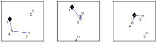
Figure 2: The three graphs $\mathcal{G}_{1},\mathcal{G}_{2},\mathcal{G}_{3}$ that comprises $\mathbb{G}$. Node $1$ is the reference.

In this scenario the nodes move in such a way that the graph $\mathcal{G}(k)$ can be one of only $3$ graphs shown in Figure 2. The graphs change according to a Markov chain whose transition probability matrix is

$$\mathcal{P}=\begin{bmatrix}0.3&0&0.7\\ 0.1&0.5&0.4\\ 0&0.5&0.5\end{bmatrix}.$$ (29)

Notice that none of the graphs is a connected graph, though the union of the graphs in $\mathbb{G}$ is connected. Also, $\mathcal{P}$ is ergodic. The mean and variance of measurement noise on every edge are chosen as $0$ and $10^{-4}$, respectively. The limiting means and variances of the estimates therefore can be computed from the predictions of Lemma 6. Monte-Carlo experiments are conducted to empirically estimate the mean and variance of the estimation error, by averaging over $1000$ sample runs.

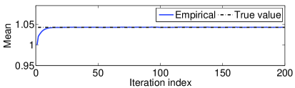
(a) Mean

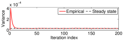
(b) Variance

Figure 3: Mean and variance of the estimate of node $3$’s node variable as a function of time. The empirical estimate of mean and variance is computed from $1000$ Monte Carlo experiments. In $(b)$, the “steady-state” corresponds to the limiting standard deviation predicted by Lemma 6.

Figure 3(a) and Figure 3(b) show the empirically estimated mean and variance of node $3$’s estimate of its node variable. As predicted by Theorem 2, the mean of the estimate converges to the true value, since the measurement noise is $0$ mean. The variance also converges to the theoretical steady state variance as predicted by Lemma 6.

5.2 A 100-node network with RWP mobility model

Here $100$ nodes move in a $1000\;m\times 1000\;m$ square according to the widely used Random Waypoint (RWP) mobility model [27]. It has been justified in the Appendix A that the graph switching process in this mobility model can be reasonably modeled as a (first order) Markov chain. The parameters maximum/minimum speed and pause time are $v_{min}=10~{}m/s$, $v_{max}=50~{}m/s$, and $t_{p}=0.1s$. The communication range is chosen as $100\;m$, and a link failure probability of $0.1$ is used. The mean and variance of the measurement noise are chosen as $0$ and $10^{-4}$. Figure 4 shows two snapshots of the network during one of the simulations. Figure 5 shows the time trace of the estimates of two nodes in one of the simulations. The mean and variance of the estimation error was empirically computed from $1000$ Monte Carlo simulations. Figure 6 shows mean and variance of the estimation error for two nodes. The figure suggests that the estimates of the node variables converge in the mean square sense. Note that the transition probability matrix is not known and the large state space makes it infeasible to compute the theoretical predictions of limiting mean and variances that are given in Lemma 6. One purpose of these simulations is therefore to test the performance of the algorithm when theoretical predictions are not available.

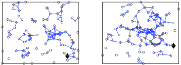
Figure 4: Two graphs that occur during a simulation with $100$ nodes moving according to the random waypoint mobility model.

\psfrag{history}{$\hat{x}_{u}(k)$}\psfrag{iteration index}{iteration index $k$}\includegraphics[scale={0.5}]{fg_one_exp_skew.eps}

Figure 5: The estimates of two nodes in one of the numerical experiments involving the $100$-node mobile network.

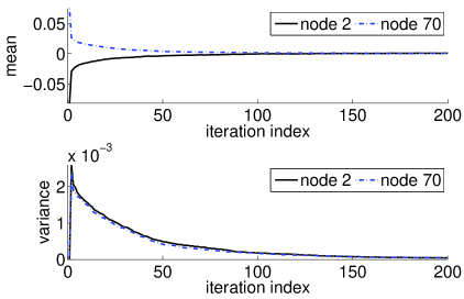
Figure 6: Empirically estimated mean and variance of the estimation error for one of the nodes in the 100-node mobile network.

6 Summary

We analyzed a distributed algorithm for estimation of clock skew and offset of the nodes of a mobile network and examined its convergence properties. The algorithm allows nodes to put different weights on estimates received from distinct neighbors, depending on the accuracy of the corresponding relative measurements. The time variation of the network was modeled as a Markov chain, which makes the algorithm a jump linear system. Under the assumptions that the Markov chain is ergodic and the diagonal entries of its transition probability matrix are positive, the estimates were shown to be mean square convergent as long as the union of the graphs over time is connected.

Expressions for the asymptotic mean and correlation are also provided by using results from jump linear systems from [19]. Evaluating these expressions requires summation of $N$ terms, where $N$ is the number of distinct graphs that can occur. In general $N$ is a very large number, so the utility of these expressions is limited in the general setting. For instance, if no restriction is placed on the motion of the nodes or edge formation, $N$ is the number of distinct graphs possible with $n$ nodes, which is $2^{\frac{1}{2}n(n-1)}$. Clearly, this is a very large number unless $n$ is extremely small. However, in special situations $N$ can be smaller, e.g., if certain nodes are restricted to move only within certain geographic areas.

In time-varying systems, the rate of change is an important parameter. The assumption that Markov chain satisfies $p_{ii}>0$ provides an upper bound on how fast nodes can move and the network can change (compared to the time required to obtain relative measurements and current estimates). This assumption was used to prove Theorem 2. However, it is possible that mean square convergence can be proved with weaker constraints on the speed of topology change.

We have not examined the question of convergence rate. It is likely that the transition probabilities of the chain will play a role in the convergence rate. However, precisely characterizing of the convergence rate of the algorithm remains an open problem. The time to reach acceptable estimation accuracy can however be reduced by more careful choice of the initial condition, e.g., using the flagged initialization scheme proposed in [11].

Appendix A Markovian model of topology change

Here we examine the question of the applicability of the Markovian model of graph switching. An example in which the time variation of the graphs satisfies the homogeneous Markov model is a network of mobile agents whose motion is modeled with first order dynamics with range-determined communication. In ad-hoc networks literature this is referred to as the random walk mobility model [27]. Specifically, suppose the position of node $u$ at time $k$, denoted by $p_{u}(k)$, is restricted to lie on the unit sphere $\mathbf{S}^{2}=\{x\in\mathbb{R}^{3}|\|x\|=1\}$, and suppose the position evolution obeys: $p_{u}(k+1)=f(p_{u}(k)+\Delta_{u}(k))$, where $\Delta_{u}(k)$ is a stationary zero-mean white noise sequence for every $u$, and $\operatorname{E}[\Delta_{u}(k)\Delta_{v}(k)^{T}]=0$ unless $u=v$. The function $f(\cdot):\mathbb{R}^{3}\to\mathbf{S}^{2}$ is a projection function onto the unit-sphere. In addition, $(u,v)\in{\mathpzc{E}}(k)$ if and only if the geodesic distance between them is less than or equal to some predetermined value. In this case, the graph $\mathcal{G}(k)$ is uniquely determined by the node positions at time $k$, and the prediction of $\mathcal{G}(k+1)$ given $\mathcal{G}(k)$ cannot be improved by the knowledge of the graphs observed prior to $k$: $\mathcal{G}(k-1),\dots,\mathcal{G}(0)$. Hence the evolution of the graph sequence satisfies the Markovian property. If in addition random communication failure leads to two nodes not being able to communicate even when they are in range, the Markovian property is retained if the communication failure is i.i.d.

However, it is not straightforward to check if the sequence of graphs generated by the model satisfies the Markovian property for other mobility models. A general method of checking Markovian switching of graphs is therefore needed. We borrow a method that is proposed in [28] to check if a stochastic process is Markov from observations of the process. We first introduce some standard notation from information theory. Let $X$ be a discrete random variable with sample space $\Omega=\{1,\dots,N\}$ and probability mass function $p(x)=P(X=x)$, where $x\in\Omega$. The entropy of $X$ is defined by

$$H(X)=-\sum_{x\in\Omega}p(x)\log\ p(x).$$ (30)

The definition of entropy is extended to a pair of random variable $X,Y$, where $X,Y\in\Omega$, as follows

$$H(X,Y):=-\sum_{x,y\in\Omega}p(x,y)\log\ p(x,y).$$ (31)

The conditional entropy $H(Y|X)$ is defined as

$$H(Y|X):=-\sum_{x,y\in\Omega}p(x,y)\log\ p(x|y)=H(X,Y)-H(X),$$ (32)

where $p(x,y)$ is joint probability mass function. The conditional entropy measures the conditional uncertainty about an event given the another event. Consider a stochastic process $\{X_{1},X_{2},\dots\}$. Assuming the process is stationary, we denote $H(single):=H(X_{k})$ and $H(double):=H(X_{k},X_{k+1})$, for all $k=1,\dots$. It is straightforward to show that $H(double)=2H(single)$ if the successive random variables $X_{k}$ are i.i.d. In this case the random process is a zero-order Markov process. If the random variables $X_{k}$ are not independent, $H<H(double)<2H$. To address the question of whether it is ($m$-th order) Markov, we extend the entropy definition to multivariate random variables, with $H(triple):=H(X_{k},X_{k+1},X_{k+2})$, etc. Now, the sequence $H_{0}=\log(N)$, $H_{1}=H(single)$, $H_{2}=H(double)-H(single)$ and $H_{3}=H(triple)-H(double)$, etc, measures the conditional uncertainty for each order of dependence. A graphical approach is given in [28] to determine the order of dependence of a random process by plotting the estimates of each $H_{i}$, where $i=1,2,\dots$ and examining the shape of the curve.

\psfrag{H}{$\hat{H}_{i}$}\includegraphics[scale={0.2}]{markov_check_0.eps}

(a) Independent

\psfrag{H}{$\hat{H}_{i}$}\includegraphics[scale={0.2}]{markov_check_1.eps}

(b) First-order

\psfrag{H}{$\hat{H}_{i}$}\includegraphics[scale={0.2}]{markov_check_2.eps}

(c) Second-order

Figure 7: The standard shapes of estimated conditional entropy for three different cases: 7(a) independence, 7(b) first-order dependence and 7(c) second-order dependence. If a process is a first order Markov chain, empirically computed conditional entropy will show a trend similar to the one in (b).

The estimate of each $H_{i}$ can be calculated from observations. Figure 7 shows the standard shapes for independence, first-order dependency, and second-order dependency. If the process is independent, then knowing the value of $X_{k}$ will not help in predicting $X_{k+1}$, which is seen in the flat shape of the entropy function in Figure 7(a). In contrast, the sharp drop from $\hat{H}_{1}$ to $\hat{H}_{2}$ in Figure 7(b) indicates that knowing the value of $X_{k-1}$ will dramatically decrease the uncertainty in the prediction of $X_{k}$, while the values of $X_{k-2},X_{k-3},\dots$ will not help much. This accords with the dependence property of a first-order Markov chain. Similarly, Figure 7(c) indicates that the previous two variables $X_{k-2},X_{k-1}$ are both important to predict $X_{k}$. In this case the process is better modeled as a second order Markov chain.

In order to conclude whether the evolution of graphs is governed by a first-order Markov chain, we adopt the method discussed above as follows. For a particular mobility model, we conduct a simulation and collect observations of the graph sequence. Since the underlying sample space $\mathbb{G}$ of the stochastic process $\mathcal{G}(k)$ is finite, the method described above is applicable. We then use the approach above to check whether the plot of $\hat{H}_{i}$ estimated from the collected observations is closer to that in Figure 7(b) than to those in Figure 7(a) or Figure 7(c). If so, we declare that it is reasonable to model the graph switching process as Markovian.

As an illustrative example, we consider the widely used random waypoint (RWP) mobility model [27]. In the RWP model, each node is initialized to stay in its initial position for a certain period of time (so called pause time $t_{p}$). Then, the node picks a random destination within the region it is allowed to move and a speed that is uniformly distributed in $[v_{min},v_{max}]$. Once node reaches the new destination, it pauses again for $t_{p}$ before starting over. We conduct a simulation of the RWP model with 3 nodes, where $v_{min}$, $v_{max}$, $t_{p}$ are chosen as $10\;m/s$, $50\;m/s$ and $0.1\;s$. The nodes are allowed to move in a region $10\times 10$ m. Nodes’ positions are initialized randomly. The sample space consists of $8$ graphs. By performing the simulation for a long time ($10^{4}\;s$), we obtain a large number of observations of the process $\{\mathcal{G}(k)\}$. The probability mass function is empirically estimated from the observations. For estimating conditional entropies, certain conditional probabilities, especially those of the type $P(\mathcal{G}(k)=G_{1}|\mathcal{G}(k-1)=G_{2},\mathcal{G}(k-2)=G_{3})$, are problematic since the relevant events may not be observed even in a very long sequence of observations. In this case we set the corresponding probabilities to $0$ and use $0\log 0=0$. The empirically estimated conditional entropies $\hat{H}_{i}$ are shown in Figure 8. Clearly, the shape of curve is similar to that in Figure 7(b). Therefore, we conclude that the graph switching process in RWP mobility can be reasonably modeled as a (first order) Markov chain.

\psfrag{H}{$\hat{H}_{i}$}\includegraphics[scale={0.25}]{markov_check.eps}

Figure 8: Empirically estimated conditional entropy for the graph process $\{\mathcal{G}_{k}\}$ with three nodes moving according to the random waypoint mobility model.

Note that in RWP mobility, prediction of the future node locations (and therefore the graph) based on knowledge of past and present may be more accurate instead of prediction based on only the present. Therefore it is quite possible that the graph switching is not first-order Markov. However, the results of the test above shows that a Markov model quite accurately captures the graph switching process with RWP mobility.

Appendix B Proof of Lemma 5

Recall that a non-negative matrix is called stochastic matrix if each row sum is $1$. If $X$ is a stochastic matrix, then $\rho(X)=1$ [31].

Proposition 7.

1. If $X$ is stochastic matrix, $X\otimes X$ is also a stochastic matrix.

2. The matrices $J_{i}$ and $F_{i}$, $i=1,\dots,N$, defined in (23) are stochastic matrices.

3. Let

   $$K :=\left(\begin{array}[]{cccc}F_{1}&F_{2}&\cdots&F_{N}\\ F_{1}&F_{2}&\cdots&F_{N}\\ \vdots&\vdots&\ddots&\vdots\\ F_{1}&F_{2}&\cdots&F_{N}\\ \end{array}\right)_{Nn^{2}\times Nn^{2}}, K_{b} :=\left(\begin{array}[]{cccc}F_{b1}&F_{b2}&\cdots&F_{bN}\\ F_{b1}&F_{2}&\cdots&F_{bN}\\ \vdots&\vdots&\ddots&\vdots\\ F_{b1}&F_{b2}&\cdots&F_{bN}\\ \end{array}\right)_{Nn_{b}^{2}\times Nn_{b}^{2}},$$

   There exists a permutation matrix $X$ so that $K_{b}$ is a principal sub-matrix of $X^{T}KX$.

4. For the matrix $\mathcal{D}$ defined in (25), $\rho(\mathcal{D})\leq 1$.

Proof: The first two statements are straightforward to establish. The third statement follows from the fact that $J_{bi}$ is a principal submatrix of $J_{i}$. We therefore prove only the fourth statement. From (24), $\rho(\mathcal{D})=\rho([p_{ji}F_{j}])$. Since $p_{ji}F_{j}$ is a non-negative square matrix, it follows from [32, Theorem 3.2] that $\rho([p_{ji}F_{j}])\leq\rho([\|p_{ji}F_{j}\|_{\infty}])$. Moreover, $\|p_{ji}F_{j}\|_{\infty}=p_{ji}\|F_{j}\|_{\infty}$. Since $F_{j}$ is a stochastic matrix, $\|F_{j}\|_{\infty}=1$. We therefore have

$$\rho(\mathcal{D})\leq\rho([p_{ji}\|F_{j}\|_{\infty}])=\rho([p_{ji}])=\rho(\mathcal{P}^{T})=\rho(\mathcal{P})=1. \square$$

Lemma 8.

Let $\mathcal{P}$ be the transition probability matrix of an $N$-state ergodic Markov chain whose diagonal entries are positive. The $\mathcal{D}$ defined in (24) is irreducible if and only if the union graph $\hat{\mathcal{G}}$ defined in (13) is connected.

The proof of Lemma 8 is postponed and we first prove Lemma 5.

Proof of Lemma 5 Since the union graph $\hat{\mathcal{G}}$ is connected, it follows from Lemma 8 that $\mathcal{D}$ is irreducible. From the third statement of Proposition 7, there exists a permutation matrix $X$, such that $\mathcal{D}_{b}$ is a principal submatrix of $X^{T}\mathcal{D}X$. The spectral radius of an irreducible matrix is strictly greater than the spectral radius of any of its principal submatrices, which follows from Theorem 5.1 in [31]. Therefore we have

$$\rho(\mathcal{D}_{b})<\rho(X^{T}\mathcal{D}X).$$

From the fourth statement in Proposition 7 and the fact that permutation does not change eigenvalues, it follows that

$$\rho(X^{T}\mathcal{D}X)=\rho(\mathcal{D})\leq 1.$$

Combining these two inequalities we get that if $\hat{\mathcal{G}}$ is connected then $\rho(\mathcal{D}_{b})<1$. To prove necessity, we construct a counterexample, in particular, a trivial Markov chain with a single state: $\mathbb{G}=\{\mathcal{G}_{1}\}$ (so that $\mathcal{P}=1$) where $\mathcal{G}_{1}$ is a $n$-node graph without any connected edge. Then $\mathcal{D}_{b}=F_{b1}=J_{b1}\otimes J_{b1}=I$, which has a spectral radius of unity. This completes the proof of the lemma. $\square$

The proof of Lemma 8 needs the following definition and results. All matrices are non-negative hereafter; so we will explicitly say “non-negative” only when we have to stress it. For matrices $X_{1},X_{2}$ of same dimension, we say $X_{1}$ and $X_{2}$ are congruent, and write $X_{1}\cong X_{2}$, if the following holds: ${(X_{1})}_{\imath\jmath}\neq 0$ if and only if ${(X_{2})}_{\imath\jmath}\neq 0$. We also write $X_{1}\succeq X_{2}$ if the following condition is satisfied: ${(X_{1})}_{\imath\jmath}\neq 0$ if ${(X_{2})}_{\imath\jmath}\neq 0$. The directed graph $\vec{G}(X)=({\mathpzc{V}}(X),\vec{{\mathpzc{E}}}(X))$ corresponding to a square matrix $X\in\mathbb{R}^{n\times n}$ is a graph defined on $n$ nodes in which $(u,v)\in\vec{{\mathpzc{E}}}(X)$ if and only if $X_{u,v}\neq 0$. A directed graph $\vec{G}$ is called strongly connected if for each pair of nodes $u$ and $v$, there is a sequence of directed edges in $\vec{{\mathpzc{E}}}$ leading from $u$ to $v$ [33]. If $\vec{G}_{1}$ is a subgraph of $\vec{G}_{2}$, meaning that $\vec{G}_{2}$ contains all the nodes and edges of $\vec{G}_{1}$, we write $\vec{G}_{1}\subseteq\vec{G}_{2}$ or $\vec{G}_{2}\supseteq\vec{G}_{1}$. Two directed graphs $\vec{G}_{1}$ and $\vec{G}_{2}$ are called congruent if their adjacency matrices are congruent. We denote by $Adj(\vec{G})$ the adjacency matrix of the graph $\vec{G}$. For a $n\times n$ square matrix $X$, we write $Adj(X)$ to denote $Adj(\vec{G}(X))$, which is an $n\times n$ matrix with $\imath,\jmath$-th entry equal to $1$ if and only if $X_{\imath\jmath}>0$, and $0$ otherwise. Essentially, the matrix $Adj(X)$ replaces the positive entries of $X$ by $1$ and leaves the $0$ entries untouched.

The following statements for non-negative matrices can be verified in a straightforward manner. All the matrices are of the same dimension.

Proposition 9.

1. $X\cong Adj(X)$.

2. $\vec{G}(X_{1})\cong\vec{G}(X_{2})$ if and only if $X_{1}\cong X_{2}$.

3. $\vec{G}(X_{1})\supseteq\vec{G}(X_{2})$ if $X_{1}\succeq X_{2}$.

4. $\vec{G}(\sum_{i}^{\ell}X_{i})\cong\cup_{i=1}^{\ell}\vec{G}(X_{i})$.

Proposition 10.

The graph $\vec{G}(X)$ is strongly connected if and only if $X$ is irreducible. If $\vec{G}(X)$ is strongly connected, then $\vec{G}(X\otimes X)$ is also strongly connected and thus $X\otimes X$ is irreducible.

The first statement of the proposition is well-known [33, pp.671]. The second statement follows from the first in a straightforward manner.

Now we define the Cartesian product of two directed graphs $\vec{G}_{1}=({\mathpzc{V}}_{1},\vec{{\mathpzc{E}}}_{1})$ and $\vec{G}_{2}=({\mathpzc{V}}_{2},\vec{{\mathpzc{E}}}_{2})$, which is denoted by $\vec{G}_{1}\Box\vec{G}_{2}$. The Cartesian product has the vertex set equal to ${\mathpzc{V}}_{1}\times{\mathpzc{V}}_{2}$, so that nodes in the product are denoted by the pair $(u,v)$, with $u\in{\mathpzc{V}}_{1}$ and $v\in{\mathpzc{V}}_{2}$, which is not to be confused with an edge. In order to prevent confusion, we will denote an edge from $u$ to $v$ in the sequel by $u\rightarrow v$. The edge set of the Cartesian product is characterized by the following property: there is an edge $(u_{1},v_{1})\rightarrow(u_{2},v_{2})$ in $\vec{G}_{1}\Box\vec{G}_{2}$ if either $u_{1}=u_{2}$ and $v_{1}\rightarrow v_{2}\in\vec{{\mathpzc{E}}}_{2}$ or $v_{1}=v_{2}$ and $u_{1}\rightarrow u_{2}\in\vec{E}_{1}$. Cartesian products of undirected graphs $\mathcal{G}_{1}$ and $\mathcal{G}_{2}$ are similarly defined, except that the resulting product graph is also undirected. The following properties will be useful in future.

Proposition 11.

1. If $\vec{G}_{1}$ and $\vec{G}_{2}$ are strongly connected, so is $\vec{G}_{1}\Box\vec{G}_{2}$.

2. If $Adj(X_{1})$ and $Adj(X_{2})$ are symmetric, then,

   $$Adj(\vec{G}(X_{1})\Box\vec{G}(X_{2}))=Adj(X_{1})\otimes I+I\otimes Adj(X_{2}).$$ (33)

Proof of Proposition 11 The first statement is from [34, Table 2]. To prove the second statement, we introduce the notation $G(X)$, which is the undirected graph corresponding to a symmetric matrix $X$. It follows that $Adj(\vec{G}(X_{1})\Box\vec{G}(X_{2}))=Adj(G(Adj(X_{1}))\Box G(Adj(X_{2})))$. From [35, Section 2.3], $Adj(G(Adj(X_{1}))\Box G(Adj(X_{2})))=Adj(X_{1})\otimes I+I\otimes Adj(X_{2})$. Thus, we prove (33). $\square$

The following results will be useful in the proof of Lemma 8.

Proposition 12.

If the union graph $\hat{\mathcal{G}}=\cup_{i=1}^{N}\mathcal{G}_{i}$ is connected, then $\cup_{i=1}^{N}\vec{G}(F_{i})$ is strongly connected.

Proof of Proposition 12 Recall that $F_{i}=J_{i}\otimes J_{i}$, where $J_{i}=(M_{i}+D_{i})^{-1}(N_{i}+D_{i})$. Since $M_{i}+D_{i}$, and therefore its inverse, is a diagonal matrix with positive entries, $J_{i}\cong(N_{i}+D_{i})$. By property 2 of Proposition 9,

$$\cup_{i=1}^{N}\vec{G}(F_{i}) \cong\vec{G}(\sum_{i=1}^{N}F_{i})\cong\vec{G}\left(\sum_{i=1}^{N}\{(N_{i}+D_{i})\otimes(N_{i}+D_{i})\}\right)$$ (34)

We also have

$$(N_{i}+D_{i})\otimes(N_{i}+D_{i}) \succeq D_{i}\otimes N_{i}+N_{i}\otimes D_{i}$$ (35)

by dropping two terms in the expansion using their non-negativity. Since $D_{i}\cong I$, we get

$$(N_{i}+D_{i})\otimes(N_{i}+D_{i}) \succeq I\otimes N_{i}+N_{i}\otimes I$$

$$\Rightarrow\sum_{i=1}^{N}\left((N_{i}+D_{i})\otimes(N_{i}+D_{i})\right) \succeq I\otimes\left(\sum_{i=1}^{N}N_{i}\right)+\left(\sum_{i=1}^{N}N_{i}\right)\otimes I.$$

Using property 3 in Proposition 9, we have

$$\cup_{i=1}^{N}\vec{G}(F_{i}) \supseteq\vec{G}\left((\sum_{i=1}^{N}N_{i})\otimes I+I\otimes(\sum_{i=1}^{N}N_{i})\right)\cong\vec{G}(\sum_{i=1}^{N}N_{i})\Box\vec{G}(\sum_{i=1}^{N}N_{i}).$$ (36)

where the congruence follows from the second statement in Proposition 11. Recall the structure of $N_{i}$, it follows that (i) $Adj(\mathcal{G}_{i})=Adj(N_{i})$, and (ii)$Adj(N_{i})$ is symmetric. As a result, $Adj(\sum_{i=1}^{N}N_{i})$ is also symmetric. Since $\hat{\mathcal{G}}=\cup_{i=1}^{N}\mathcal{G}_{i}$ is a connected undirected graph, its adjacency matrix is irreducible. This means $Adj(\cup_{i=1}^{N}\mathcal{G}_{i})=\sum_{i=1}^{N}Adj(\mathcal{G}_{i})=\sum_{i=1}^{N}Adj(N_{i})$ is irreducible. Due to the first statement in Proposition 11, $\vec{G}(\sum_{i=1}^{N}N_{i})\Box\vec{G}(\sum_{i=1}^{N}N_{i})$ is strongly connected. The result of this proposition now follows from (36). $\square$

The Kronecker product of two graphs $\vec{G}_{1}=({\mathpzc{V}}_{1},\vec{{\mathpzc{E}}}_{1})$ and $\vec{G}_{2}=({\mathpzc{V}}_{2},\vec{{\mathpzc{E}}}_{2})$, denoted by $\vec{G}_{1}\otimes\vec{G}_{2}$, has the vertex set equal to $\vec{V}_{1}\times\vec{V}_{2}$ and an edge set that is characterized by the following property: there is an edge $(u_{1},v_{1})\rightarrow(u_{2},v_{2})$ in $\vec{G}_{1}\otimes\vec{G}_{2}$ if and only if $u_{1}\rightarrow u_{2}\in\vec{{\mathpzc{E}}}_{1}$ and $v_{1}\rightarrow v_{2}\in\vec{{\mathpzc{E}}}_{2}$ [34]. Note that the Cartesian and Kronecker products $\vec{G}_{1}\Box\vec{G}_{2}$ and $\vec{G}_{1}\otimes\vec{G}_{2}$ have the same vertex sets but distinct edge sets. We have the following property of Kronecker product of graphs from [36]:

$$Adj(\vec{G}_{1}\otimes\vec{G}_{2})=Adj(\vec{G}_{1})\otimes Adj(\vec{G}_{2}).$$ (37)

Adjacency matrices of both Cartesian and Kronecker products of two graphs are related to the adjacency matrices of the individual graphs through the matrix Kronecker product, cf. (33) and (37).

Now we are ready to prove the Lemma 8. Proof of Lemma 8 (Connectivity $\Rightarrow$ irreducibility): Here we have to prove that if the union graph $\hat{\mathcal{G}}$ is connected then the matrix $\mathcal{D}$ is irreducible. We will prove it by showing that the directed graph $\vec{\mathcal{G}}(\mathcal{D})$ is strongly connected. Let $Z_{j}$ and $S_{j}$ be the diagonal and off-diagonal parts of $F_{j}$. Since $Z_{i}$ is a non-negative matrix with positive diagonal, we get

$$\mathcal{D} \cong[p_{ji}Z_{j}]+[p_{ji}S_{j}]\cong[p_{ji}I_{n^{2}}]+[p_{ji}S_{j}]$$

$$\succeq\mathcal{P}^{T}\otimes I+diag[p_{ii}S_{i}]$$ (38)

where we have used the fact that $[p_{ji}I_{n^{2}}]=\mathcal{P}^{T}\otimes I$ and dropped the off-diagonal blocks of $[p_{ji}S_{j}]$. Therefore

$$\vec{\mathcal{G}}(\mathcal{D}) \supseteq\vec{G}(\mathcal{P}^{T}\otimes I)\bigcup\vec{G}(diag[S_{i}])$$

$$=\{\vec{G}(\mathcal{P}^{T})\otimes\vec{G}(I)\}\bigcup\vec{G}(diag[S_{i}])$$

where the equality follows from the property (37) of Kronecker product of graphs. We will now show that the directed graph $\{\vec{G}(\mathcal{P}^{T})\otimes\vec{G}(I)\}\bigcup\vec{G}(diag[S_{i}])$ is strongly connected, which proves that $\vec{\mathcal{G}}(\mathcal{D})$ is as well.

First notice that there are $Nn^{2}$ nodes in the graph $\vec{\mathcal{G}}(\mathcal{D})$, so are $\mathcal{P}^{T}\otimes I$ and $diag[S_{i}]$. It is convenient to imagine them as $N\times N$ block matrices, with each block being of dimension $n^{2}\times n^{2}$. Therefore, we introduce a useful new notation. Let’s index a node by the pair $(p_{i},d_{\kappa})$, which is the $((i-1)N+\kappa)$-th node in $\vec{\mathcal{G}}(\mathcal{D})$, where $i=1,\dots,N$ and $\kappa=1,\dots,n^{2}$. This notation is similarly suitable for $\mathcal{P}^{T}\otimes I$ and $diag[S_{i}]$. To prove that $\{\vec{G}(\mathcal{P}^{T})\otimes\vec{G}(I)\}\bigcup\vec{G}(diag[S_{i}])$ is strongly connected, we need to show the following

$$\text{\emph{There is a path from an arbitrary node}}(p_{i},d_{\kappa})\text{\emph{to another arbitrary node}}(p_{j},d_{\nu})$$

$$\text{ \emph{in the graph} }\{\vec{G}(\mathcal{P}^{T})\otimes\vec{G}(I)\}\bigcup\vec{G}(diag[S_{i}]).$$ (39)

The following properties will be used to construct a proof of (B):

1. s1: There exists a path from $(p_{i},d_{\kappa})$ to $(p_{j},d_{\kappa})$ in $\vec{G}(\mathcal{P}^{T}\otimes I)$ for all $i,j=1,\dots,N$ and $\kappa=1,\dots,n^{2}$.

2. s2: If $d_{\kappa}\rightarrow d_{h}$ is an edge in $\vec{\mathcal{G}}(S_{\ell})$, then $(p_{\ell},d_{\kappa})\rightarrow(p_{\ell},d_{h})$ is an edge in $\vec{\mathcal{G}}(diag[S_{i}])$.

The first statement is proved as follows. Since the Markov chain is ergodic, $\mathcal{P}$ - and therefore $\mathcal{P}^{T}$ - is irreducible, which means $\vec{\mathcal{G}}(\mathcal{P}^{T})$ is strongly connected. Thus, given arbitrary nodes $p$ and $q$ in $\vec{\mathcal{G}}(\mathcal{P}^{T})$, there is a path connecting them in $\vec{\mathcal{G}}(\mathcal{P}^{T})$. Call this path $p,u_{1},u_{2},\dots,u_{m},q$. Since the edge $d_{\kappa}\rightarrow d_{\kappa}\in\vec{\mathcal{G}}(I)$ exists for every $\kappa$, it now follows from the definition of Kronecker product of graphs that the path $(p,d_{\kappa}),(u_{1},d_{\kappa}),(u_{2},d_{\kappa}),\dots,(u_{m},d_{\kappa}),(q,d_{\kappa})$ exists in $\vec{G}(\mathcal{P}^{T})\otimes\vec{G}(I)$ for every $\kappa=1,\dots,n^{2}$. The statement s1 is now proved upon replacing $p$ and $q$ by $p_{i}$ and $p_{j}$. The statement s2 is true because of the structure of the matrix $diag[S_{i}]$ and the node indexing scheme described immediately before (B).

From Proposition 12, we have that $\cup_{i=1}^{N}\vec{G}(\bar{F}_{i})$ is connected. Since $S_{i}$ is the off-diagonal part of $\bar{F}_{i}$, $\cup_{i=1}^{N}\vec{G}(S_{i})$ is connected as well. Therefore, there is a path from an arbitrary node $d_{\kappa}$ to another arbitrary node $d_{\nu}$ in $\cup_{i=1}^{N}\vec{G}(S_{i})$, for all $\kappa,\nu$ in $\{1,\dots,n^{2}\}$. To prove the statement (B), pick such a path from the node $d_{\kappa}$ to the node $d_{\nu}$ in $\cup_{i=1}^{N}\vec{G}(S_{i})$, where each edge in the path may lie in any of the graphs $\{\vec{G}(S_{i})\}_{i=1}^{N}$. For the sake of concreteness and compactness, let us consider a path of length two, consisting of the two edges $d_{\kappa}\rightarrow d_{h}$ and $d_{h}\rightarrow d_{\nu}$, which belong to the graphs, say, $\vec{G}(S_{\ell})$ and $\vec{G}(S_{m})$, respectively. From s1 we have proved above, we know that there is a path from the node $(p_{i},d_{\kappa})$ to the node $(p_{\ell},d_{\kappa})$ in the graph $\vec{\mathcal{G}}(\mathcal{P}^{T}\otimes I)$, call this path $path[(p_{i},d_{\kappa})\leadsto(p_{\ell},d_{\kappa})]$. From s2, we have that the edge $(p_{\ell},d_{\kappa})\rightarrow(p_{\ell},d_{h})$ exists in the graph $\vec{\mathcal{G}}(diag[S_{i}])$ due to the existence of the edge $d_{\kappa}\rightarrow d_{h}$ in $\vec{\mathcal{G}}(S_{\ell})$. Thus, we have the path from $(p_{i},d_{\kappa})$ to $(p_{\ell},d_{h})$ in the combined graph $\{\vec{G}(\mathcal{P}^{T})\otimes\vec{G}(I)\}\bigcup\vec{G}(diag[S_{i}])$ by joining the path $path[(p_{i},d_{\kappa})\leadsto(p_{\ell},d_{\kappa})]$ with the edge $(p_{\ell},d_{\kappa})\rightarrow(p_{\ell},d_{h})$. Using this idea repeatedly, we construct a path from $(p_{i},d_{\kappa})$ to $(p_{j},d_{\nu})$ in $\{\vec{G}(\mathcal{P}^{T})\otimes\vec{G}(I)\}\bigcup\vec{G}(diag[S_{i}])$ as follows:

$$path[(p_{i},d_{\kappa})\leadsto(p_{\ell},d_{\kappa})], \quad\text{ in }\vec{G}(\mathcal{P}^{T})\otimes\vec{G}(I)$$

$$(p_{\ell},d_{\kappa})\rightarrow(p_{\ell},d_{h}), \quad\in\vec{G}(diag[S_{i}])$$

$$path[(p_{\ell},d_{h})\leadsto(p_{m},d_{h})], \quad\text{ in }\vec{G}(\mathcal{P}^{T})\otimes\vec{G}(I)$$

$$(p_{m},d_{h})\rightarrow(p_{m},d_{\nu}), \quad\in\vec{G}(diag[S_{i}])$$

$$path[(p_{m},d_{\nu})\leadsto(p_{j},d_{\nu})], \quad\text{ in }\vec{G}(\mathcal{P}^{T})\otimes\vec{G}(I),$$

where each $path[\cdot]$ exists due to the property s1 established above, and each edge exists due to the property s2 as well as with the assumed existence of the edges $d_{\kappa}\rightarrow d_{h}$ and $d_{h}\rightarrow d_{\nu}$ in the union graph. This argument can be extended to a path of any length between $d_{\kappa}$ and $d_{\nu}$ in the union graph $\cup_{i=1}^{N}\vec{G}(S_{i})$. Thus, there is a path from $(p_{i},d_{\kappa})$ to $(p_{j},d_{\nu})$ in $\{\vec{G}(\mathcal{P}^{T})\otimes\vec{G}(I)\}\bigcup\vec{G}(diag[S_{i}])$, which proves sufficiency.

(Not connected $\Rightarrow$ reducible): A simple counterexample proves necessity. Construct a trivial Markov chain with a single state: $\mathbb{G}=\{\mathcal{G}_{1}\}$ (so that $\mathcal{P}=1$) where $\mathcal{G}_{1}$ is an $n$-node graph without a single edge. Then $\mathcal{D}=F_{1}=J_{1}\otimes J_{1}=I$, which is reducible. $\square$

References

- [1] F. Sivrikaya and B. Yener, “Time synchronization in sensor networks: a survey,” IEEE Network, vol. 18, no. 4, pp. 45 – 50, july-aug. 2004.
- [2] B. Sundararaman, U. Buy, and A. D. Kshemkalyani, “Clock synchronization for wireless sensor networks: a survey,” Ad Hoc Networks, vol. 3, no. 3, pp. 281 – 323, 2005.
- [3] B. M. Sadler and A. Swami, “synchronization in sensor networks: an overview,” in IEEE MILCOM, October 2006, pp. 1–6.
- [4] K.-L. Noh, Q. M. Chaudhari, E. Serpedin, and B. W. Suter, “Novel clock phase offset and skew estimation using two-way timing message exchanges for wireless sensor networks,” IEEE Transactions on Communications, vol. 55, no. 4, pp. 766–777, Apr 2007.
- [5] S. Yoon, C. Veerarittiphan, and M. L. Sichitiu, “Tiny-sync: Tight time synchronization for wireless sensor networks,” ACM Transactions on Sensor Networks, vol. 3, no. 2, pp. 1–34, Jun 2007.
- [6] M. Leng and Y.-C. Wu, “On clock synchronization algorithms for wireless sensor networks under unknown delay,” IEEE Transactions on Vehicular Technology, vol. 59, no. 1, pp. 182–190, Jan 2010.
- [7] Y.-C. Wu, Q. Chaudhari, and E. Serpedin, “Clock synchronization of wireless sensor networks,” IEEE Signal Processing Magazine, vol. 28, no. 1, pp. 124 –138, jan. 2011.
- [8] S. Ganeriwal, R. Kumar, and M. B. Srivastava, “Timing-sync protocol for sensor networks,” in ACM Conference on Embedded Networked Sensor Systems (SenSys), 2003.
- [9] M. Maróti, B. Kusy, G. Simon, and Á. Lédeczi, “The flooding time synchronization protocol,” in ACM Conference on Embedded Networked Sensor Systems (SenSys), 2004.
- [10] P. Barooah and J. P. Hespanha, “Distributed optimal estimation from relative measurements,” in Proceedings of the 3rd International Conference on Intelligent Sensing and Information Processing (ICISIP), December 2005, pp. 226–231.
- [11] P. Barooah, N. M. da Silva, and J. P. Hespanha, “Distributed optimal estimation from relative measurements for localization and time synchronization,” in Distributed Computing in Sensor Systems DCOSS, ser. LNCS, P. B. Gibbons, T. Abdelzaher, J. Aspnes, and R. Rao, Eds. Springer, 2006, vol. 4026, pp. 266 – 281.
- [12] R. Solis, V. S. Borkar, and P. R. Kumar, “A new distributed time synchronization protocol for multihop wireless networks,” in Proc. of the 45th IEEE Conference on Decison and Control, December 2006, pp. 2734–2739.
- [13] N. Freris, V. Borkar, and P. Kumar, “A model-based approach to clock synchronization,” in Decision and Control, 2009 held jointly with the 2009 28th Chinese Control Conference. CDC/CCC 2009. Proceedings of the 48th IEEE Conference on, dec. 2009, pp. 5744 –5749.
- [14] M. Leng and Y.-C. Wu, “Distributed clock synchronization for wireless sensor networks using belief propagation,” Signal Processing, IEEE Transactions on, vol. 59, no. 11, pp. 5404 –5414, nov. 2011.
- [15] R. Carli and S. Zampieri, “Networked clock synchronization based on second order linear consensus algorithms,” in Decision and Control (CDC), 2010 49th IEEE Conference on, dec. 2010, pp. 7259 –7264.
- [16] R. Carli, E. D’Elia, and S. Zampieri, “A pi controller based on asymmetric gossip communications for clocks synchronization in wireless sensors networks,” in Decision and Control and European Control Conference (CDC-ECC), 2011 50th IEEE Conference on, dec. 2011, pp. 7512 –7517.
- [17] L. Schenato and F. Fiorentin, “Average timesynch: A consensus-based protocol for clock synchronization in wireless sensor network,” Automatica, vol. 47, no. 9, pp. 1878 – 1886, 2011.
- [18] R. Karp, J. Elson, D. Estrin, and S. Shenker, “Optimal and global time synchronization in sensornets,” Center for Embedded Networked Sensing, Univ. of California, Los Angeles, Tech. Rep., 2003.
- [19] O. Costa, M. Fragoso, and R. Marques, Discrete-Time Markov Jump Linear Systems, ser. Probability and its Applications. Springer, 2004.
- [20] S. Kar and J. Moura, “Distributed consensus algorithms in sensor networks with imperfect communication: Link failures and channel noise,” Signal Processing, IEEE Transactions on, vol. 57, no. 1, pp. 355 –369, jan. 2009.
- [21] M. Huang, S. Dey, G. N. Nair, and J. H. Manton, “Stochastic consensus over noisy networks with Markovian and arbitrary switches,” Automatica, vol. 46, no. 10, pp. 1571–1583, Oct. 2010.
- [22] T. Li and J. Zhang, “Consensus conditions of multi-agent systems with time-varying topologies and stochastic communication noises,” Automatic Control, IEEE Transactions on, vol. 55, no. 9, pp. 2043–2057, 2010.
- [23] J. Liu, X. Liu, W.-C. Xie, and H. Zhang, “Stochastic consensus seeking with communication delays,” Automatica, vol. 47, no. 12, pp. 2689 – 2696, 2011.
- [24] V. Gupta, B. Hassibi, and R. M. Murray, “Stability analysis of stochastically varying formations of dynamic agents,” in Proceedings. of the 42nd IEEE Conference on Decision and Control, vol. 1, dec. 2003, pp. 504 – 509.
- [25] Y. Zhang and Y.-P. Tian, “Consentability and protocol design of multi-agent systems with stochastic switching topology,” Automatica, vol. 45, no. 5, pp. 1195 – 1201, 2009.
- [26] S. Kar and J. M. F. Moura, “Distributed consensus algorithms in sensor networks: Quantized data and random link failures,” IEEE Transactions on Signal Processing, vol. 58, no. 3, p. 1383–1400, March 2010.
- [27] T. Camp, J. Boleng, and V. Davies, “A survey of mobility models for ad hoc network research,” Wireless Communications and Mobile Computing, vol. 2, no. 5, pp. 483–502, Aug 2002.
- [28] C. Chatfield, “Statistical Inference Regarding Markov Chain Models,” Applied Statistics, vol. 22, no. 1, pp. 7–20, 1973.
- [29] C. Liao and P. Barooah, “Time synchronization in mobile sensor networks from difference measurements,” in In proceedings of the 49th IEEE Conference on Decision and Control, December 2010, pp. 2118 – 2123.
- [30] K.-L. Noh, E. Serpedin, and K. Qaraqe, “A new approach for time synchronization in wireless sensor networks: Pairwise broadcast synchronization,” IEEE Transaction on Wireless Communications, vol. 7, no. 9, pp. 3318–3322, Sep 2008.
- [31] H. Minc, Nonnegative Matrices. Wiley-Interscience, 1988.
- [32] M.-Q. Chen and X. Li, “An estimation of the spectral radius of a product of block matrices,” Linear Algebra and its Applications, March 2004.
- [33] C. D. Meyer, Matrix Analysis and Applied Linear Algebra. SIAM: Society for Industrial and Applied Mathematics, 2001.
- [34] F. Harary and J. Trauth, Charles A., “Connectedness of products of two directed graphs,” SIAM Journal on Applied Mathematics, vol. 14, no. 2, pp. pp. 250–254, 1966.
- [35] B. Yackley, E. Corona, and T. Lane, “Bayesian network score approximation using a metagraph kernel 21,” in Advances in Neural Information Processing Systems, D. Koller, D. Schuurmans, Y. Bengio, and L. Bottou, Eds., 2009, pp. 1833–1840.
- [36] P. M. Weichsel, “The kronecker product of graphs,” Proceedings of the American Mathematical Society, vol. 13, no. 1, pp. pp. 47–52, 1962.