Effects of enhanced stratification on equatorward dynamo wave propagation

Abstract

We present results from simulations of rotating magnetized turbulent convection in spherical wedge geometry representing parts of the latitudinal and longitudinal extents of a star. Here we consider a set of runs for which the density stratification is varied, keeping the Reynolds and Coriolis numbers at similar values. In the case of weak stratification, we find quasi-steady dynamo solutions for moderate rotation and oscillatory ones with poleward migration of activity belts for more rapid rotation. For stronger stratification, the growth rate tends to become smaller. Furthermore, a transition from quasi-steady to oscillatory dynamos is found as the Coriolis number is increased, but now there is an equatorward migrating branch near the equator. The breakpoint where this happens corresponds to a rotation rate that is about 3–7 times the solar value. The phase relation of the magnetic field is such that the toroidal field lags behind the radial field by about $\pi/2$, which can be explained by an oscillatory $\alpha^{2}$ dynamo caused by the sign change of the $\alpha$-effect about the equator. We test the domain size dependence of our results for a rapidly rotating run with equatorward migration by varying the longitudinal extent of our wedge. The energy of the axisymmetric mean magnetic field decreases as the domain size increases and we find that an $m=1$ mode is excited for a full $2\pi$ azimuthal extent, reminiscent of the field configurations deduced from observations of rapidly rotating late-type stars.

1. Introduction

The large-scale magnetic field of the Sun, manifested by the 11 year sunspot cycle, is generally believed to be generated within or just below the turbulent convection zone (e.g., Ossendrijver, 2003, and references therein). The latter concept is based on the idea that strong shear in the tachocline near the bottom of the convection zone amplifies the toroidal magnetic field which then becomes buoyantly unstable and erupts to the surface (e.g., Parker, 1955b). This process has been adopted in many mean-field models of the solar cycle in the form of a non-local $\alpha$-effect (e.g., Kitchatinov & Olemskoy, 2012), which is based on early ideas of Babcock (1961) and Leighton (1969) that the source term for poloidal field can be explained through the tilt of active regions. Such models assume a reduced turbulent diffusivity within the convection zone and a single cell anti-clockwise meridional circulation which acts as a conveyor belt for the magnetic field. These so-called flux transport models (e.g., Dikpati & Charbonneau, 1999) are now widely used to study the solar cycle and to predict its future course (Dikpati & Gilman, 2006; Choudhuri et al., 2007).

The flux transport paradigm is, however, facing several theoretical challenges: $10^{5}$ gauss magnetic fields are expected to reside in the tachocline (D’Silva & Choudhuri, 1993), but such fields are difficult to explain with dynamo theory (Guerrero & Käpylä, 2011) and may have become unstable at much lower field strengths (Arlt et al., 2005). Furthermore, flux transport dynamos require a rather low value of the turbulent diffusivity within the convection zone (several $10^{11}\,{\rm cm}^{2}\,{\rm s}^{-1}$; see Bonanno et al., 2002), which is much less than the standard estimate of several $10^{12}\,{\rm cm}^{2}\,{\rm s}^{-1}$ based on mixing length theory, which, in turn, is also verified numerically (e.g., Käpylä et al., 2009). Several other issues have already been addressed within this paradigm, for example, the parity of the dynamo (Bonanno et al., 2002; Chatterjee et al., 2004; Dikpati et al., 2004) and the possibility of a multicellular structure of the meridional circulation (Jouve & Brun, 2007), which may be more complicated than that required in the flux transport models (Hathaway, 2011; Miesch et al., 2012; Zhao et al., 2013). These difficulties have led to a revival of the distributed dynamo (e.g., Brandenburg, 2005; Pipin, 2013) in which magnetic fields are generated throughout the convection zone due to turbulent effects (e.g., Krause & Rädler, 1980; Käpylä et al., 2006b; Pipin & Seehafer, 2009).

Early studies of self-consistent three-dimensional magnetohydrodynamic (MHD) simulations of convection in spherical coordinates produced oscillatory large-scale dynamos (Gilman, 1983; Glatzmaier, 1985), but the dynamo wave was found to propagate toward the poles rather than the equator—as in the Sun. These models are referred to as direct numerical simulations (DNS), i.e., all operators of viscous and diffusive terms are just the original ones, but with vastly increased viscosity and diffusivity coefficients. More recent anelastic large-eddy simulations (LES) with rotation rates somewhat higher than that of the Sun have produced non-oscillatory (Brown et al., 2010) and oscillatory (Brown et al., 2011; Nelson et al., 2013) large-scale magnetic fields, depending essentially on the rotation rate and the vigor of the turbulence. However, similar models with the solar rotation rate have either failed to produce an appreciable large-scale component (Brun et al., 2004) or, more recently, oscillatory solutions with almost no latitudinal propagation of the activity belts (Ghizaru et al., 2010; Racine et al., 2011). These simulations covered a full spherical shell and used realistic values for solar luminosity and rotation rate, necessitating the use of anelastic solvers and spherical harmonics (e.g., Brun et al., 2004) or implicit methods (e.g. Ghizaru et al., 2010). Here we exploit an alternative approach by modeling fully compressible convection in wedge geometry (see also Robinson & Chan, 2001) with a finite-difference method. We omit the polar regions and usually cover only a part of the longitudinal extent, e.g., $90\arcdeg$ instead of the full $360\arcdeg$. At the cost of omitting connecting flows across the poles and introducing artificial boundaries there, the gain is that higher spatial resolution can be achieved. Furthermore, retaining the sound waves can be beneficial when considering possible helio- or asteroseismic applications. Our model is a hybrid between DNS and LES in that we supplement the thermal energy flux by an additional subgrid scale (SGS) term to stabilize the scheme and to further reduce the radiative background flux. Recent hydrodynamic (Käpylä et al., 2011a, b) and MHD (Käpylä et al., 2010b) studies have shown that this approach produces results that are in accordance with fully spherical models. Moreover, the first turbulent dynamo solution with solar-like migration properties of the magnetic field was recently obtained using this type of setup (Käpylä et al., 2012). Extended setups that include a coronal layer as a more realistic upper radial boundary have been successful in producing dynamo-driven coronal ejections (Warnecke et al., 2012). As we show in a companion paper (Warnecke et al., 2013), a solar-like differential rotation pattern might be another consequence of including an outer coronal layer.

Here we concentrate on exploring further the recent discovery of equatorward migration in spherical wedge simulations (Käpylä et al., 2012). In particular, we examine a set of runs for which the rotational influence on the fluid, measured by the Coriolis number, which is also called the inverse Rossby number, is kept approximately constant while the density stratification of the simulations is gradually increased.

2. The model

Our model is the same as that in Käpylä et al. (2012). We consider a wedge in spherical polar coordinates, where $(r,\theta,\phi)$ denote radius, colatitude, and longitude. The radial, latitudinal, and longitudinal extents of the wedge are $r_{0}\leq r\leq R$, $\theta_{0}\leq\theta\leq\pi-\theta_{0}$, and $0\leq\phi\leq\phi_{0}$, respectively, where $R$ is the radius of the star and $r_{0}=0.7\,R$ denotes the position of the bottom of the convection zone. Here we take $\theta_{0}=\pi/12$ and in most of our models we use $\phi_{0}=\pi/2$, so we cover a quarter of the azimuthal extent between $\pm 75^{\circ}$ latitude. We solve the compressible hydromagnetic equations,

$$\frac{\partial\bm{A}}{\partial t}={\bm{u}}\times{\bm{B}}-\mu_{0}\eta{\bm{J}},$$ (1)

$$\frac{D\ln\rho}{Dt}=-\bm{\nabla}\cdot\bm{u},$$ (2)

$$\frac{D\bm{u}}{Dt}=\bm{g}-2\bm{\Omega}_{0}\times\bm{u}+\frac{1}{\rho}\left(\bm{J}\times\bm{B}-\bm{\nabla}p+\bm{\nabla}\cdot 2\nu\rho\bm{\mathsf{S}}\right),$$ (3)

$$T\frac{Ds}{Dt}=\frac{1}{\rho}\left[-\bm{\nabla}\cdot\left({\bm{F}^{\rm rad}}+{\bm{F}^{\rm SGS}}\right)+\mu_{0}\eta{\bm{J}}^{2}\right]+2\nu\bm{\mathsf{S}}^{2},$$ (4)

where ${\bm{A}}$ is the magnetic vector potential, $\bm{u}$ is the velocity, ${\bm{B}}=\bm{\nabla}\times{\bm{A}}$ is the magnetic field, ${\bm{J}}=\mu_{0}^{-1}\bm{\nabla}\times{\bm{B}}$ is the current density, $\mu_{0}$ is the vacuum permeability, $D/Dt=\partial/\partial t+\bm{u}\cdot\bm{\nabla}$ is the advective time derivative, $\rho$ is the density, $\nu$ is the kinematic viscosity, $\eta$ is the magnetic diffusivity, both assumed constant,

$${\bm{F}^{\rm rad}}=-K\bm{\nabla}T\quad\mbox{and}\quad{\bm{F}^{\rm SGS}}=-\chi_{\rm SGS}\rho T\bm{\nabla}s$$ (5)

are radiative and SGS heat fluxes, where $K$ is the radiative heat conductivity and $\chi_{\rm SGS}$ is the turbulent heat conductivity, which represents the unresolved convective transport of heat and was referred to as $\chi_{\rm t}$ in Käpylä et al. (2012), $s$ is the specific entropy, $T$ is the temperature, and $p$ is the pressure. The fluid obeys the ideal gas law with $p=(\gamma-1)\rho e$, where $\gamma=c_{\rm P}/c_{\rm V}=5/3$ is the ratio of specific heats at constant pressure and volume, respectively, and $e=c_{\rm V}T$ is the specific internal energy. The rate of strain tensor $\bm{\mathsf{S}}$ is given by

$$\mathsf{S}_{ij}={\textstyle{1\over 2}}(u_{i;j}+u_{j;i})-{\textstyle{1\over 3}}\delta_{ij}\bm{\nabla}\cdot\bm{u},$$ (6)

where the semicolons denote covariant differentiation (Mitra et al., 2009).

The gravitational acceleration is given by $\bm{g}=-GM\hat{\bm{r}}/r^{2}$, where $G$ is the gravitational constant, $M$ is the mass of the star (without the convection zone), and $\hat{\bm{r}}$ is the unit vector in the radial direction. Furthermore, the rotation vector $\bm{\Omega}_{0}$ is given by $\bm{\Omega}_{0}=(\cos\theta,-\sin\theta,0)\Omega_{0}$.

2.1. Initial and boundary conditions

The initial state is isentropic and the hydrostatic temperature gradient is given by

$$\frac{\partial T}{\partial r}=-\frac{GM/r^{2}}{c_{\rm V}(\gamma-1)(n_{\rm ad}+1)},$$ (7)

where $n_{\rm ad}=1.5$ is the polytropic index for an adiabatic stratification. We fix the value of $\partial T/\partial r$ on the lower boundary. The density profile follows from hydrostatic equilibrium. The heat conduction profile is chosen so that radiative diffusion is responsible for supplying the energy flux in the system, with $K$ decreasing more than two orders of magnitude from bottom to top (Käpylä et al., 2011a). We do this by choosing a variable polytropic index $n=2.5\,(r/r_{0})^{-15}-1$, which equals 1.5 at the bottom of the convection zone and approaches $-1$ closer to the surface. This means that $K=(n+1)K_{0}$ decreases toward the surface like $r^{-15}$ such that most of the flux is carried by convection (Brandenburg et al., 2005). Here, $K_{0}$ is a constant that will be defined below.

Our simulations are defined by the energy flux imposed at the bottom boundary, $F_{\rm b}=-(K\partial T/\partial r)|_{r=r_{0}}$ as well as the values of $\Omega_{0}$, $\nu$, $\eta$, and $\overline{\chi}_{\rm SGS}=\chi_{\rm SGS}(r_{\rm m}=0.85\,R)$. Furthermore, the radial profile of $\chi_{\rm SGS}$ is piecewise constant above $r>0.75R$ with $\chi_{\rm SGS}=\overline{\chi}_{\rm SGS}$ at $0.75<r<0.98$, and $\chi_{\rm SGS}=12.5\overline{\chi}_{\rm SGS}$ above $r=0.98R$. Below $r=0.75R$, $\chi_{\rm SGS}$ tends smoothly to zero; see Fig. 1 of Käpylä et al. (2011a).

The radial and latitudinal boundaries are assumed to be impenetrable and stress free, i.e.,

$$\!\!\!u_{r}=0,\quad\frac{\partial u_{\theta}}{\partial r}=\frac{u_{\theta}}{r},\quad\frac{\partial u_{\phi}}{\partial r}=\frac{u_{\phi}}{r}\quad(r=r_{0},R),$$ (8)

$$\!\!\!\frac{\partial u_{r}}{\partial\theta}=u_{\theta}=0,\quad\frac{\partial u_{\phi}}{\partial\theta}=u_{\phi}\cot\theta\quad(\theta=\theta_{0},\pi-\theta_{0}).\quad$$ (9)

For the magnetic field we assume perfect conductors on the latitudinal and lower radial boundaries, and radial field on the outer radial boundary. In terms of the magnetic vector potential these translate to

$$\!\!\!\frac{\partial A_{r}}{\partial r}=A_{\theta}=A_{\phi}=0\,\quad(r=r_{0}),$$ (10)

$$\!\!\!A_{r}=0,\;\;\frac{\partial A_{\theta}}{\partial r}=-\frac{A_{\theta}}{r},\;\;\frac{\partial A_{\phi}}{\partial r}=-\frac{A_{\phi}}{r}\quad(r=R),\quad$$ (11)

$$\!\!\!A_{r}=\frac{\partial A_{\theta}}{\partial\theta}=A_{\phi}=0\quad(\theta=\theta_{0},\pi-\theta_{0}).$$ (12)

We use small-scale low amplitude Gaussian noise as initial condition for velocity and magnetic field. On the latitudinal boundaries we assume that the density and entropy have vanishing first derivatives, thus suppressing heat fluxes through the boundaries.

On the upper radial boundary we apply a black body condition

$$\sigma T^{4}=-K\nabla_{r}T-\chi_{\rm SGS}\rho T\nabla_{r}s,$$ (13)

where $\sigma$ is the Stefan–Boltzmann constant. We use a modified value for $\sigma$ that takes into account that both surface temperature and energy flux through the domain are larger than in the Sun. The value of $\sigma$ can be chosen so that the flux at the surface carries the total luminosity through the boundary in the initial non-convecting state. However, in many cases we have changed the value of $\sigma$ during runtime to speed up thermal relaxation.

2.2. Dimensionless parameters

To facilitate comparison with other work using different normalizations, we present our results by normalizing with physically meaningful quantities. We note, however, that in the code we used non-dimensional quantities by choosing

$$R=GM=\rho_{0}=c_{\rm P}=\mu_{0}=1,$$ (14)

where $\rho_{0}$ is the initial density at $r=r_{0}$. The units of length, time, velocity, density, entropy, and magnetic field are therefore

$$[x]=R,\,\,\,[t]=\sqrt{R^{3}/GM},\,\,\,[u]=\sqrt{GM/R},$$

$$[\rho]=\rho_{0},\,\,\,[s]=c_{\rm P},\,\,\,[B]=\sqrt{\rho_{0}\mu_{0}GM/R}.$$ (15)

The radiative conductivity is proportional to $K_{0}=(\mathcal{L}/4\pi)c_{\rm V}(\gamma-1)(n_{\rm ad}+1)\rho_{0}\sqrt{GMR}$, where $\mathcal{L}$ is the non-dimensional luminosity, given below. The corresponding nondimensional input parameters are the luminosity parameter

$$\mathcal{L}=\frac{L_{0}}{\rho_{0}(GM)^{3/2}R^{1/2}},$$ (16)

the normalized pressure scale height at the surface,

$$\xi=\frac{(\gamma-1)c_{\rm V}T_{1}}{GM/R},$$ (17)

with $T_{1}$ being the temperature at the surface, the Taylor number

$${\rm Ta}=(2\Omega_{0}R^{2}/\nu)^{2},$$ (18)

the fluid and magnetic Prandtl numbers

$${\rm Pr}=\frac{\nu}{\chi_{\rm m}},\quad{\rm Pr}_{\rm SGS}=\frac{\nu}{\overline{\chi}_{\rm SGS}},\quad{\rm Pm}=\frac{\nu}{\eta},$$ (19)

where $\chi_{\rm m}=K/c_{\rm P}\rho_{\rm m}$ and $\rho_{\rm m}$ are the thermal diffusivity and density at $r=r_{\rm m}$, respectively. Finally, we have the non-dimensional viscosity

$$\tilde{\nu}=\frac{\nu}{\sqrt{GMR}}.$$ (20)

Instead of $\xi$, we often quote the initial density contrast, $\Gamma_{\rho}^{(0)}\equiv\rho(r_{0})/\rho(R)$. The density contrast can change during the run. We list the final values of $\Gamma_{\rho}$ from the thermally saturated stage in Table 1.

Other useful diagnostic parameters are the fluid and magnetic Reynolds numbers

$${\rm Re}=\frac{u_{\rm rms}}{\nu k_{\rm f}},\quad{\rm Rm}=\frac{u_{\rm rms}}{\eta k_{\rm f}},$$ (21)

where $k_{\rm f}=2\pi/\Delta r\approx 21R^{-1}$ is an estimate of the wavenumber of the largest eddies, and $\Delta r=R-r_{0}=0.3\,R$ is the thickness of the layer. The Coriolis number is defined as

$${\rm Co}=\frac{2\Omega_{0}}{u_{\rm rms}k_{\rm f}},$$ (22)

where $u_{\rm rms}=\sqrt{(3/2)\langle u_{r}^{2}+u_{\theta}^{2}\rangle_{r\theta\phi t}}$ is the rms velocity and the subscripts indicate averaging over $r$, $\theta$, $\phi$, and a time interval during which the run is thermally relaxed and which covers several magnetic diffusion times. The averaging procedures employ the correct volume or surface elements of spherical polar coordinates. Note that for $u_{\rm rms}$ we omit the contribution from the azimuthal velocity, because its value is dominated by effects from the differential rotation (Käpylä et al., 2011b) and compensate for this with the $3/2$ factor. The Taylor number can also be written as ${\rm Ta}={\rm Co}^{2}{\rm Re}^{2}(k_{\rm f}R)^{4}$. Due to the fact that the initial stratification is isentropic, we quote the turbulent Rayleigh number ${\rm Ra}_{\rm t}$ from the thermally relaxed state of the run,

$${\rm Ra}_{\rm t}\!=\!\frac{GM(\Delta r)^{4}}{\nu\overline{\chi}_{\rm SGS}R^{2}}\bigg{(}-\frac{1}{c_{\rm P}}\frac{{\rm d}\langle s\rangle_{\theta\phi t}}{{\rm d}r}\bigg{)}_{r_{\rm m}}.$$ (23)

We also quote the value of $k_{\omega}=\omega_{\rm rms}/u_{\rm rms}$, where $\bm{\omega}=\bm{\nabla}\times{\bm{u}}$, and $\omega_{\rm rms}$ is the volume averaged rms value of $\bm{\omega}$. The magnetic field is expressed in equipartition field strengths, $B_{\rm eq}(r)=\langle\mu_{0}\rho\bm{u}^{2}\rangle^{1/2}_{\theta\phi t}$, where all three components of $\bm{u}$ are included. We define mean quantities as averages over the $\phi$-coordinate and denote them by overbars. However, as we will see, there can also be significant power in non-axisymmetric spherical harmonic modes with low azimuthal degree $m=1$ and 2, which will be discussed at the end of the paper.

The simulations were performed with the Pencil Code, which uses a high-order finite difference method for solving the compressible equations of magnetohydrodynamics.

Table 1Summary of the runs.

Run	grid	${\rm Pr}$	${\rm Pr}_{\rm SGS}$	${\rm Pm}$	$\mbox{Ta}[10^{10}]$	$\xi$	$\Gamma_{\rho}^{(0)}$	$\Gamma_{\rho}$	$\tilde{\nu}[10^{-5}]$	$\mathcal{L}[10^{-5}]$	$\tilde{\sigma}$	${\rm Ra}_{\rm t}[10^{6}]$	${\rm Re}$	${\rm Rm}$	${\rm Co}$
A1	$128\times 256\times 128$	71	$1.5$	$1.0$	$1.0$	0.29	2.0	2.1	$1.7$	$3.8$	$0.92$	$0.83$	$26$	$26$	$8.6$
A2	$128\times 256\times 128$	71	$1.5$	$1.0$	$1.8$	0.29	2.0	2.1	$1.7$	$3.8$	$0.92$	$0.11$	$24$	$24$	$12.8$
B1	$128\times 256\times 128$	82	$2.5$	$1.0$	$0.64$	0.09	5.0	5.3	$2.9$	$3.8$	$10.9$	$1.1$	$22$	$22$	$8.1$
B2	$128\times 256\times 128$	82	$2.5$	$1.0$	$1.4$	0.09	5.0	5.2	$2.9$	$3.8$	$10.9$	$1.1$	$20$	$20$	$13.7$
C1	$128\times 256\times 128$	56	$2.5$	$1.0$	$1.4$	0.02	30	22	$2.9$	$3.8$	$1.4\cdot 10^{3}$	$2.1$	$35$	$35$	$7.8$
C2	$128\times 256\times 128$	56	$2.5$	$1.0$	$4.0$	0.02	30	21	$2.9$	$3.8$	$1.4\cdot 10^{3}$	$2.7$	$31$	$31$	$14.8$
D1	$128\times 256\times 128$	503	$7.5$	$3.0$	$0.16$	0.008	100	85	$4.7$	$0.63$	$3.9\cdot 10^{4}$	$1.2$	$11$	$34$	$8.0$
D2	$256\times 512\times 256$	269	$4.0$	$2.0$	$1.0$	0.008	100	74	$2.5$	$0.63$	$3.9\cdot 10^{4}$	$2.4$	$25$	$50$	$9.1$
E1	$128\times 256\times 64$	56	$2.5$	$1.0$	$1.4$	0.02	30	22	$2.9$	$3.8$	$1.4\cdot 10^{3}$	$2.1$	$34$	$34$	$7.9$
E2	$128\times 256\times 128$	56	$2.5$	$1.0$	$1.4$	0.02	30	22	$2.9$	$3.8$	$1.4\cdot 10^{3}$	$2.1$	$35$	$35$	$7.8$
E3	$128\times 256\times 256$	56	$2.5$	$1.0$	$1.4$	0.02	30	22	$2.9$	$3.8$	$1.4\cdot 10^{3}$	$2.4$	$35$	$35$	$7.9$
E4	$128\times 256\times 512$	67	$3.0$	$1.0$	$1.0$	0.02	30	23	$3.5$	$3.8$	$1.4\cdot 10^{3}$	$2.2$	$28$	$28$	$8.1$

Note. — Columns 2–7 and 9–11 show quantities that are input parameters to the models whereas the quantities in the eight and the last four columns are results of the simulations computed from the saturated state. Here we use $\phi_{0}=\pi/2$ in Sets A–D. In Set E we use $\phi_{0}=\pi/4$ (Run E1), $\phi_{0}=\pi/2$ (E2), $\phi_{0}=\pi$ (E3), and $\phi_{0}=2\pi$ (E4). Runs C1 and E2 are the same model, which is also the same as Run B4m of Käpylä et al. (2012). Here $\Gamma_{\rho}$ is the density stratification in the final saturated state and $\tilde{\sigma}=\sigma R^{2}T_{0}^{4}/L_{0}$, where $T_{0}$ is the temperature at the base of the convection zone.

Table 2Summary of diagnostic variables.

Run	$\tilde{\lambda}$	$\tilde{u}_{\rm rms}$	$E_{\rm mer}/E_{\rm kin}$	$E_{\rm rot}/E_{\rm kin}$	$E_{\rm mag}/E_{\rm kin}$	$E_{\rm pol}/E_{\rm mag}$	$E_{\rm tor}/E_{\rm mag}$	$\Delta_{\Omega}^{(r)}$	$\Delta_{\Omega}^{(\theta)}$	$k_{\omega}$
A1	0.084	0.010	0.000	0.580	0.418	0.045	0.396	0.013	0.089	62
A2	0.095	0.009	0.000	0.490	0.553	0.068	0.338	0.009	0.050	62
B1	0.028	0.013	0.000	0.705	0.345	0.038	0.487	0.034	0.142	68
B2	0.098	0.012	0.000	0.757	0.222	0.056	0.427	0.023	0.072	72
C1	0.006	0.021	0.001	0.440	0.346	0.138	0.203	0.047	0.068	93
C2	0.105	0.019	0.001	0.326	0.706	0.198	0.238	0.016	0.030	94
D1	0.003	0.011	0.002	0.222	0.472	0.166	0.135	0.011	-0.000	89
D2	0.003	0.013	0.000	0.617	0.222	0.133	0.190	0.045	0.058	116
E1	0.007	0.021	0.001	0.478	0.393	0.133	0.328	0.048	0.069	92
E2	0.006	0.021	0.001	0.440	0.346	0.138	0.203	0.047	0.068	93
E3	0.005	0.021	0.001	0.375	0.380	0.120	0.172	0.037	0.055	92
E4	0.024	0.020	0.001	0.410	0.477	0.016	0.080	0.028	0.054	89

Note. — Here $\tilde{\lambda}=\lambda/(u_{\rm rms}k_{\rm f})$ is the normalized growth rate of the magnetic field and $\tilde{u}_{\rm rms}=u_{\rm rms}/\sqrt{GM/R}$ is the non-dimensional rms velocity. $E_{\rm kin}={\textstyle{1\over 2}}\langle\rho{\bm{u}}^{2}\rangle$ is the volume averaged kinetic energy. $E_{\rm mer}={\textstyle{1\over 2}}\langle\rho(\overline{u}_{r}^{2}+\overline{u}_{\theta}^{2})\rangle$ and $E_{\rm rot}={\textstyle{1\over 2}}\langle\rho\overline{u}_{\phi}^{2}\rangle$ denote the volume averaged energies of the azimuthally averaged meridional circulation and differential rotation. Analogously $E_{\rm mag}={\textstyle{1\over 2}}\langle{\bm{B}}^{2}\rangle$ is the total volume averaged magnetic energy while $E_{\rm pol}={\textstyle{1\over 2}}\langle(\overline{B}_{r}^{2}+\overline{B}_{\theta}^{2})\rangle$ and $E_{\rm tor}={\textstyle{1\over 2}}\langle\overline{B}_{\phi}^{2}\rangle$ are the energies in the axisymmetric part of the poloidal and toroidal magnetic fields.

2.3. Relation to reality

In simulations, the maximum possible Rayleigh number is much smaller than in real stars due to the higher diffusivities. This implies higher energy fluxes and thus larger Mach numbers (Brandenburg et al., 2005). To have realistic Coriolis numbers, the angular velocity in the Coriolis force has to be increased in proportion to one third power of the increase of the energy flux, but the centrifugal acceleration is omitted, as it would otherwise be unrealistically large (cf. Käpylä et al., 2011b). In the present models this would mean that the centrifugal acceleration is of the same order of magnitude as gravity, thus significantly altering the hydrostatic balance.

We note that we intend to use low values of $\mathcal{L}$ so that the Mach number is sufficiently below unity. This is particularly important when the stratification is strong. In our current formulation the unresolved turbulent heat conductivity, $\chi_{\rm SGS}$, acts on the total entropy and thus contributes to the radial heat flux. In the current models with ${\rm Pr}_{\rm SGS}$ greater than unity, the SGS-flux accounts for a few per cent of the total flux within the convection zone. Using smaller values of ${\rm Pr}_{\rm SGS}$ at the same Reynolds number would lead to a greater contribution due to the SGS-flux. To minimize the effects of the SGS-flux within the convection zone, we use the smallest possible value of $\chi_{\rm SGS}$ that is still compatible with numerical stability.

The span of time scales in our model is strongly compressed so as to comprise the full range all the way to the viscous, thermal, and resistive time scales. In the following we define acoustic, convective, thermal, resistive, and viscous time scales as follows:

$$\tau_{\rm ac}=\sqrt{R^{3}/GM},\quad\tau_{\rm conv}=H_{\rm P0}/u_{\rm rms}^{\rm(ref)},$$ (24)

$$\tau_{\rm th}=H_{\rm P0}^{2}/\chi_{0},\quad\tau_{\rm res}=H_{\rm P0}^{2}/\eta,\quad\tau_{\rm visc}=H_{\rm P0}^{2}/\nu,$$ (25)

where $H_{\rm P0}$ is the pressure scale height at $r_{0}$, $u_{\rm rms}^{\rm(ref)}=(F_{0}/\rho_{0})^{1/3}$ is a convective reference velocity based on the luminosity of the model, $L=4\pi r_{0}^{2}F_{0}$, and $F_{0}$ is the total flux at $r_{0}$.

A visual comparison of these different time scales for the Sun and Run C1 is given in Figure 1. In order to allow for slow thermal and resistive relaxation processes, we require that their respective time scales are shorter than the run time $T$ of the simulation. As stated in Section 2.2, the acoustic time scale of our model is equal to that of the Sun. This implies that all the other time scales must be significantly reduced: $\tau_{\rm conv}$ by a factor 70–100, $\tau_{\rm th}$ and $\tau_{\rm res}$ by a factor $10^{7}$, and $\tau_{\rm visc}$ by a factor $10^{14}$. This is accomplished by taking values of ${\cal L}$ that are not as small as in the Sun (where ${\cal L}\approx 5\times 10^{-11}$), but typically $3.8\times 10^{-5}$ for Run C1. This just corresponds to taking values of the Rayleigh number that are on the order of $10^{6}$ rather than solar values (in excess of $10^{24}$). Likewise, shorter thermal, resistive, and viscous time scales are obtained by choosing values of the magnetic and fluid Reynolds number that are not as large as in the Sun and by choosing magnetic and fluid Prandtl numbers that are not as small as in the Sun.

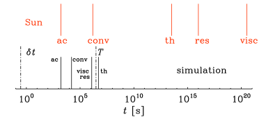
Figure 1.— Visual comparison of acoustic, convective, thermal, resistive, and viscous time scales both in the Sun (upper part, in red) and in Run C1 (lower part). In our models, resistive and viscous time scales are often equal, and the thermal time scale is 1.5–7.5 times longer; see Columns 4 and 5 of Table 1. The simulation time scales are confined between the length of the time step, $\delta t$, and the maximum run time, $T$.

For the purpose of comparing dynamo time scales of the model with the Sun, it is useful to rescale them such that $\tau_{\rm conv}$ coincides with that of the Sun. We can then compare the rotation rates of our models in Table 1 with that of the Sun: Runs A1 and A2 are 2 and 3 times solar, B1 and B2 are 3 and 4.4 times solar, C1 (including all of Set E) and C2 are 4.4 and 7 times solar, and D1 and D2 are 4.3 and 6 times solar.

3. Results

We perform runs for four values of $\xi$, corresponding to initial density contrasts $\Gamma_{\rho}^{(0)}=2,5,30$, and $100$. These runs are referred to as Sets A–D. In Set E we use $\Gamma_{\rho}^{(0)}=30$ and vary $\phi_{0}$ with all other parameters being kept the same as in Run C1, except in Run E4 where we use 20% higher viscosity and magnetic diffusivity than in the other runs in Set E. For each series, we consider different values of ${\rm Ta}$ and, as a consequence, of Co and Re. The hydrodynamic progenitors of the Runs B1, C1, and D1 correspond to Runs A4, B4, and C4, respectively, from Käpylä et al. (2011a). The rest of the simulations were run from the initial conditions described in Section 2.1.

Earlier studies applying fully spherical simulations have shown that organized large-scale magnetic fields appear provided the rotation of the star is rapid enough (Brown et al., 2010) and that at even higher rotation rates, cyclic solutions with poleward migration of the activity belts are obtained (Brown et al., 2011). A similar transition has been observed in the spherical wedge models of Käpylä et al. (2010b) and Käpylä et al. (2012). However, in the former case the oscillatory mode showed poleward migration, whereas in the latter an equatorward branch appears near the equator. Furthermore, in these runs the dynamo mode changes from one showing a high frequency cycle with poleward migration near the equator to another mode with lower frequency and equatorward migration when the magnetic field becomes dynamically important.

There are several differences between the models of Käpylä et al. (2010b) and Käpylä et al. (2012): the amount of density stratification (a density contrast of 3 in comparison to 30), the efficiency of convective energy transport (20% versus close to 100% in the majority of the domain achieved by the use of $\chi_{\rm SGS}$; see also Figure 2), and the top boundary condition for entropy (constant temperature versus black body radiation). Here we concentrate on studying the influence of the density stratification on models similar to those presented in Käpylä et al. (2012).

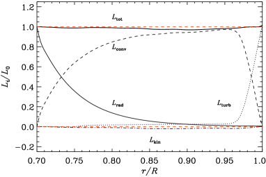
Figure 2.— Luminosity of the energy fluxes from Run E4: radiative conduction (thin solid line), enthalpy (dashed), kinetic energy (dot-dashed), and unresolved subgrid scale (dotted) fluxes. The thick solid line is the sum of all contributions. The two dashed red lines indicate the zero and unity lines.

3.1. Thermal boundary effects and energy balance

In Käpylä et al. (2011a) we started to apply the black–body boundary condition, Equation (13), that has previously been used in mean-field models with thermodynamics (Rüdiger, 1989; Brandenburg et al., 1992; Kitchatinov & Mazur, 2000). Instead of using the physical value for the Stefan–Boltzmann constant, we estimate the value of $\sigma$ so that the flux at the upper boundary is approximately that needed to transport the total luminosity of the star through the surface; see Table 1. However, the final thermally relaxed state of the simulation can significantly deviate from the initial state. In combination with the nonlinearity of Equation (13), the final stratification is usually somewhat different from the initial one; see Figure 3 for an illustrative example from Run C1. The final density stratification in this case is around 22, down from 30 in the initial state.

The main advantage of the black–body condition is that it allows the temperature at the surface more freedom than in our previous models where a constant temperature was imposed (Käpylä et al., 2010b, 2011b). In particular, as the temperature is allowed to vary at the surface, this can be used as a diagnostic for possible irradiance variations. These issues are discussed further in Section 3.8.

Considering the energy balance, we show the averaged radial energy fluxes for Run E4 in Figure 2. We find that the simulation is thermally relaxed and that the total luminosity is close to the input luminosity, i.e., $L_{\rm tot}-L_{0}\approx 0$. The fluxes are defined as:

$$\mathcal{F}_{\rm rad} = -K\langle\nabla_{r}T\rangle,$$ (26)

$$\mathcal{F}_{\rm conv} = c_{\rm P}\langle(\rho u_{r})^{\prime}T^{\prime}\rangle,$$ (27)

$$\mathcal{F}_{\rm kin} = {\textstyle{1\over 2}}\left\langle\rho u_{r}{\bm{u}}^{2}\right\rangle,$$ (28)

$$\mathcal{F}_{\rm visc} = -2\nu\left\langle\rho u_{i}S_{ir}\right\rangle,$$ (29)

$$\mathcal{F}_{\rm turb} = -\chi_{\rm SGS}\langle\rho T\nabla_{r}s\rangle,$$ (30)

$$\mathcal{F}_{\rm Poyn} = \langle E_{\theta}B_{\phi}-E_{\phi}B_{\theta}\rangle/\mu_{0},$$ (31)

where ${\bm{E}}=\eta\mu_{0}{\bm{J}}-{\bm{u}}\times{\bm{B}}$, the primes denote fluctuations, and angle brackets abbreviate $\langle\cdot\rangle_{\theta,\phi,t}$. The radiative flux carries energy into the convection zone and drops steeply as a function of radius so that it contributes only a few per cent in the middle of the convection zone. The resolved convection is responsible for transporting the energy through the majority of the layer, whereas the unresolved turbulent transport carries energy through the outer surface. The viscous and Poynting fluxes are much smaller, and are thus omitted in this figure. The flux of kinetic energy is also very small in the rapid rotation regime considered here (see also Augustson et al., 2012).

Figure 3.— Initial (solid lines) and saturated (dashed) radial profiles of temperature $T$, density $\rho$, and pressure $p$, normalized by their respective values at the bottom of the domain (indicated by the subscript zero) from Run C1. The inset shows the specific entropy $s/c_{\rm P}$ from the same run.

3.2. Dynamo excitation and large-scale magnetic fields

The azimuthally averaged toroidal magnetic fields from Sets A–D listed in Tables 1 and 2 are shown in Figures 4–7. The full time evolution from the introduction of the seed magnetic field to the final saturated state is shown for each run. Note that the magnitude of the seed field in terms of the equipartition strength is different in each set so direct comparisons between different sets are not possible. We measure the average growth rates during the kinematic stage,

$$\lambda=\langle d\ln B_{\rm rms}/dt\rangle_{t},$$ (32)

and find that $\lambda$ is greater for smaller stratification; see Column 2 of Table 2 for $\tilde{\lambda}=\lambda/(u_{\rm rms}k_{\rm f})$. Comparing Runs A1, B1, C1, and D2 with roughly comparable Reynolds and Coriolis numbers shows that the normalized growth rate decreases monotonically from 0.084 in Run A1 to just 0.003 in Run D2. Another striking feature is that $\tilde{\lambda}$ increases by a factor of nearly 20 from Run C1 to C2 whose only difference is that the latter has a roughly two times higher Coriolis number. It turns out that in all of the cases (Runs A1, A2, B1, B2, C2, and E4) with the highest growth rates, a dynamo mode with poleward migration at low latitudes, is excited first. In some of the runs this mode is later overcome by another one that can be quasi-stationary (Runs A1 and B1) or oscillatory with equatorward migration and a much longer cycle period (Runs C2 and E4).

Table 2 shows that, even though the growth rates decrease dramatically with increasing stratification, many properties of the saturated stages are similar. In particular, the ratio of magnetic to kinetic energies does not seem to systematically depend on stratification, but rather on the Coriolis number, which varies only little between different runs.

In Figure 4 we show the azimuthally averaged toroidal magnetic field $\overline{B}_{\phi}$ near the surface of the computational domain ($r=0.98\,R$) for two runs (A1 and A2; see Table 1) with $\Gamma_{\rho}^{(0)}=2$. We find that in Run A1 with ${\rm Co}\approx 8.7$ the mean magnetic field is initially oscillatory with poleward propagation of the activity belts. At $tu_{\rm rms}k_{\rm f}\approx 400$ the dynamo mode changes to a quasi-steady configuration. In Run A2 a poleward mode persists throughout the simulation, although the oscillation period is irregular and significant hemispherical asymmetry exists. This behavior is similar to Run A4 presented in Käpylä et al. (2010b) with comparable stratification ($\Gamma\approx 3$) and Reynolds ($\approx 20$) numbers, but a somewhat lower Coriolis number ($\approx 4.7$). The transition to oscillatory solutions thus occurs at a lower ${\rm Co}$ in the models of Käpylä et al. (2010b). A possible explanation is that in the present models we lack a lower overshoot layer which could affect the dominant dynamo mode.

In Set B with $\Gamma_{\rho}^{(0)}=5$ the situation is similar: in Run B1 with ${\rm Co}\approx 8.1$ there is a poleward mode near the equator with a short cycle period which is visible from early times; see Figure 5. However, after around $tu_{\rm rms}k_{\rm f}=1200$ there is a dominating non-oscillatory mode that is especially clear at high latitudes. There are still hints of the poleward mode near the equator. In Run B2 with ${\rm Co}\approx 13.7$, however, the poleward mode also prevails at late times. As in Run A2, the cycles show significant variability and hemispheric asymmetry. The runs in Sets A and B also show signs of non-axisymmetric ‘nests’ of convection (cf. Busse, 2002; Brown et al., 2008) in the hydrodynamical and kinematic stages. Once the magnetic field becomes dynamically important, these modes either vanish or they are significantly damped.

Increasing the stratification further to $\Gamma_{\rho}^{(0)}=30$ (Set C) the dynamo solutions at lower rotation rates, ${\rm Co}\lesssim 5$, are still quasi-steady; see Figure 2 of Käpylä et al. (2012). However, a watershed regarding the oscillatory modes at higher ${\rm Co}$ seems to have been reached so that the irregular poleward migration seen in Sets A and B is replaced by more regular equatorward patterns. In Run C1 with ${\rm Co}\approx 8.7$ the poleward migration near the equator is also visible in the kinematic stage where the equatorward mode is not yet excited; see Figure 6. The poleward mode near the equator is more prominent in the early stages of Run C2 with ${\rm Co}\approx 14.7$, but subdominant at late times.

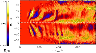
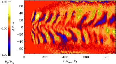
Figure 4.— $\overline{B}_{\phi}$ near the surface of the star at $r=0.98\,R$ as a function of latitude ($=90\arcdeg-\theta$) and time for Runs A1 (top) and A2 (bottom). The white dotted line denotes the equator $90\arcdeg-\theta=0$.

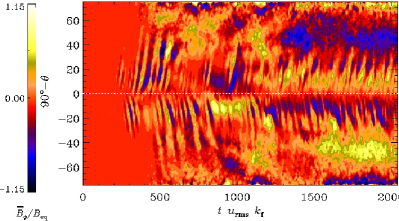
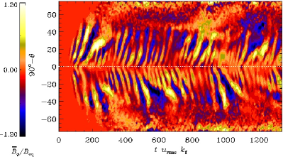
Figure 5.— Same as Figure 4, but for Runs B1 (top) and B2 (bottom).

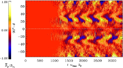
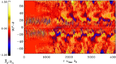
Figure 6.— Same as Figure 4, but for Runs C1 (top) and C2 (bottom). Note the difference in cycle frequency between the early times when the frequency is similar to that of Run B2 (Figure 5) and late times.

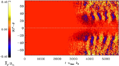
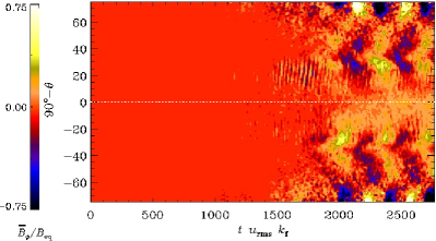
Figure 7.— Same as Figure 4, but for Runs D1 (top) and D2 (bottom).

For $\Gamma_{\rho}^{(0)}=100$ (Set D) the general picture is similar to that in Set C. Quasi-steady configurations at lower rotation rates change into equatorward migrating solutions at sufficiently high values of ${\rm Co}$. We find that this transition occurs between ${\rm Co}=5$ and $8$, similar to Set C; see Fig. 2 of Käpylä et al. (2012). For Set D the equatorward mode is visible for both of its runs; see Figure 7. In Run D1 no poleward migration at low latitudes is seen in the kinematic stage. Also, the poleward migrating branch at high latitudes is missing in the non-linear stage. Both of these features are present in Run D2. The apparently slower growth of the magnetic field in Run D1 is due to a two orders of magnitude lower seed magnetic field than in Run D2.

3.3. Diagnostic stellar activity diagrams

To identify the possibility of different types of dynamos, it is useful to classify them in diagrams relating their characteristic properties. In the geodynamo literature it has become customary to consider the Elsasser number as a measure of the magnetic energy. It correlates well with ${\rm Rm}$ (Christensen & Aubert, 2006), but this is partially explained by the fact that ${\rm Rm}$ itself enters in the definition of the Elsasser number. Geodynamo models are mostly dominated by a strong dipolar component. Gastine et al. (2012) have shown that such solutions fall on a branch that is distinct from the cyclic solutions studied here, and that the latter solutions become favored once density stratification is large and rotation is sufficiently rapid so that large-scale non-axisymmetric fields become dominant (see also Nelson et al., 2013). However, this type of analysis is not well suited for the present work, where ${\rm Rm}$ and ${\rm Co}$ vary only little. Furthermore, these tools do not characterize the nature of magnetic cycles, which is the focus of this section.

To connect our results with observations of magnetically active stars we compute the ratio of cycle to rotation frequency $\omega_{\rm cyc}/\Omega_{0}$, where $\omega_{\rm cyc}=2\pi/T_{\rm cyc}$ is the cycle frequency of magnetic energy of the mean field and $T_{\rm cyc}$ its period. Plotting this ratio as a function of the Coriolis number for stars exhibiting chromospheric activity has shown that stars tend to group along inactive and active branches (Brandenburg et al., 1998), and for higher Coriolis numbers along a super-active branch (Saar & Brandenburg, 1999). Six of our simulations (Runs A2, B2, C1, C2, D1, and D2), excluding the runs in Set E (which are very similar to each other and to Run C1), show cycles and can thus be used in this analysis. We compute the cycle frequency from the highest peak of a temporal Fourier transformation of the time series for $\overline{B}_{\phi}$ averaged over a latitudinal strip of $\pm 10\arcdeg\ldots 30\arcdeg$ near the surface. The results are shown in Figure 8(a).

Three of the models, Runs C1, D1, and D2, fall on a branch labeled ‘${\cal A}$?’ for active stars, while Run C2 might be suggestive of the superactive stars of Saar & Brandenburg (1999), labeled here ‘${\cal S}$??’. Runs A2 and B2 show irregular cycles and group along the branch labeled ‘${\cal I}$?’ for inactive stars. The question marks on these labels in Figure 8(a) indicate that the association with real branches is quite uncertain and somewhat premature, because there are too few models. We cannot be sure that there are no models connecting the group of Runs C1, D1, D2 with that of A2 and B2 through a single line with a steeper slope. Nevertheless, this plot allows us to see that, while the separation in the ratio $\omega_{\rm cyc}/\Omega_{0}$ is slightly less for the two groups of runs compared with active and inactive stars, their relative ordering in the value of ${\rm Co}$ is actually the other way around. One would therefore not have referred to Runs A2 and B2 as inactive just because their $\omega_{\rm cyc}/\Omega_{0}$ ratio agrees with that of inactive stars. In fact, their $E_{\rm mag}/E_{\rm kin}$ ratios (a measure of stellar activity) in Table 2 are typically larger than for Runs C1, D1, and D2.

As is visible from Figure 8(c), there is no clear relation between ${\rm Co}$ and $E_{\rm mag}/E_{\rm kin}$, which is different from stars for which there is a clear relation between ${\rm Co}$ (referred to as the inverse Rossby number in that context) and stellar activity; see Brandenburg et al. (1998) for details and references. Furthermore, there are also no indications of branches in the graph of $\omega_{\rm cyc}/\Omega_{0}$ versus $E_{\rm mag}/E_{\rm kin}$; see Figure 8(b). Instead, there might just be one group in it, possibly with a positive correlation, i.e., $\omega_{\rm cyc}/\Omega_{0}$ might increase with $E_{\rm mag}/E_{\rm kin}$. Such a possibility does indeed arise when considering the frequency ratio versus the dimensional rotation rate (Oláh et al., 2000). However, as discussed by Brandenburg et al. (1998), a positive slope is not easily explained in the framework of standard mean-field dynamo theory, where the frequency ratio is usually a decreasing function of normalized rotation rate and activity parameter (Tobias, 1998; Saar & Brandenburg, 1999).

In conclusion, we reiterate that the quantity $\omega_{\rm cyc}/\Omega_{0}$ is an important and robust property of cyclic dynamo models and its dependence on other properties of the model should therefore be a useful characteristics that can be compared with other models and ultimately with actual stars. Here we have made a first attempt in classifying model results in this way.

Figure 8.— Diagnostic diagrams from six runs that show cyclic activity. (a) Ratio of cycle and rotation frequencies vs. $\log{\rm Co}$. The dotted and dashed lines are given by $c_{i}{\rm Co}^{\sigma_{i}}$, where $\sigma_{i}$ correspond to those in Brandenburg et al. (1998) for active (labeled ‘${\cal A}$?’) and inactive (‘${\cal I}$?’) stars, while $c_{i}$ are used as fit parameters. The label ‘${\cal S}$??’ indicates the possibility of the superactive branch in Saar & Brandenburg (1999). (b) Ratio of cycle and rotation frequencies vs. magnetic to kinetic energy $E_{\rm mag}/E_{\rm kin}$. (c) Time averaged $E_{\rm mag}/E_{\rm kin}$ vs. $\log{\rm Co}$.

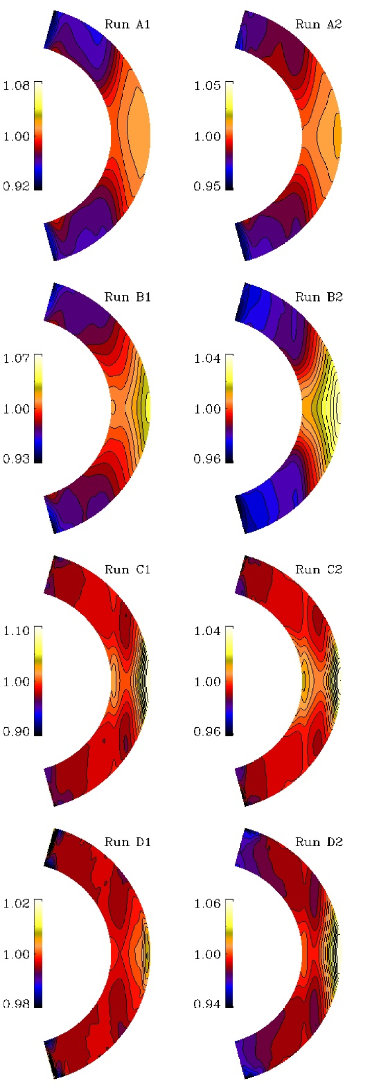
Figure 9.— Time averaged mean rotation profiles $\overline{\Omega}/\Omega_{0}$ (gray/color scale and line contours) from Sets A, B, C, and D.

3.4. Differential rotation and meridional circulation

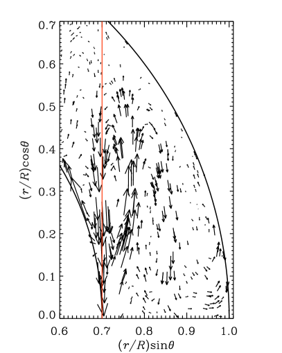
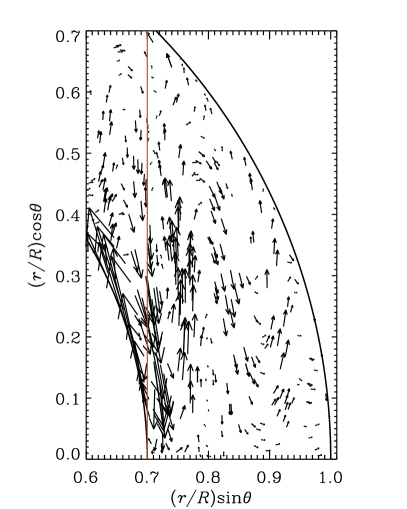
Figure 10.— Meridional circulation in the northern hemisphere of the convection zone of Run C1 (left panel) and Run D1 (right) shown as vectors of the mass flux $\overline{\rho}(\overline{u}_{r},\overline{u}_{\theta},0)$, which is also averaged over a time span of around 250 turnover times in the saturated state. The black solid lines indicate the surface ($r=R$) and the bottom of the convection zone ($r=0.7\,R$), and the red solid line indicates the position of the inner tangent cylinder. Note, that for Run D1 (right), the mass flux have been multiplied by a factor of 5 to emphasize the structure.

Non-uniform rotation of the convection zone of the Sun is an important ingredient in maintaining the large-scale magnetic field. Furthermore, the sign of the radial gradient of the mean angular velocity plays a crucial role in deciding whether the dynamo wave propagates toward the pole or the equator in $\alpha$–$\Omega$ mean-field models (e.g., Parker, 1955a, 1987b). In the following we use the local angular velocity defined as $\overline{\Omega}=\Omega_{0}+\overline{u}_{\phi}/r\sin\theta$. Azimuthally averaged rotation profiles from the runs in Sets A to D are shown in Figure 9. The rotation profiles of Runs E1, E3, and E4 are very similar to that of Run C1. We quantify the radial and latitudinal differential rotation by

$$\Delta_{\Omega}^{(r)} = \frac{\overline{\Omega}_{\rm eq}-\overline{\Omega}_{\rm bot}}{\overline{\Omega}_{\rm eq}},$$ (33)

$$\Delta_{\Omega}^{(\theta)} = \frac{\overline{\Omega}_{\rm eq}-\overline{\Omega}_{\rm pole}}{\overline{\Omega}_{\rm eq}},$$ (34)

where $\overline{\Omega}_{\rm eq}=\overline{\Omega}(R,\pi/2)$ and $\overline{\Omega}_{\rm bot}=\overline{\Omega}(r_{0},\pi/2)$ are the angular velocities at the top and bottom at the equator, respectively, and $\overline{\Omega}_{\rm pole}=[\overline{\Omega}(R,\theta_{0})+\overline{\Omega}(R,\pi-\theta_{0})]/2$. It has long been recognized that dynamo-generated magnetic fields can have an important effect on the angular velocity (Gilman, 1983; Glatzmaier, 1985, 1987). Indeed, magnetic fields affect the turbulence that gives rise to Reynolds stress and turbulent convective heat flux (e.g., Kitchatinov et al., 1994; Käpylä et al., 2004). Furthermore, the large-scale flows are directly influenced by the Lorentz force when the magnetic field is strong enough (e.g., Malkus & Proctor, 1975). A magnetically caused decrease of $\Delta_{\Omega}^{(\theta)}$ has also been observed in LES models (e.g., Brun et al., 2004). Comparing the latitudinal differential rotation in Run B1 with that of the otherwise identical hydrodynamic Run A4 of Käpylä et al. (2011a), we find that $\Delta_{\Omega}^{(\theta)}$ decreases only slightly from 0.15 to 0.14. For $\Delta_{\Omega}^{(r)}$ the change is more dramatic—from 0.079 to 0.034. The fraction of kinetic energy contained in the differential rotation, $E_{\rm rot}/E_{\rm kin}$, drops from 0.91 to 0.71. A similar decrease is observed in Run C1 in comparison to its hydrodynamical parent Run B4 of Käpylä et al. (2011a) with $\Delta_{\Omega}^{(\theta)}$ changing from 0.08 to 0.07, $\Delta_{\Omega}^{(r)}$ from 0.066 to 0.047, and $E_{\rm rot}/E_{\rm kin}$ dropping from 0.58 to 0.44. Similar changes have also been seen in dynamos from forced turbulence in Cartesian domains (Brandenburg, 2001), in addition to those from convective turbulence in spherical shells (Brun et al., 2004).

In all cases in Figure 9, we see a rapidly spinning equator with a positive radial gradient of $\overline{\Omega}$. The latitudinal variation of angular velocity is, however, not always monotonic and there can be local minima at mid-latitudes, as is seen, for example, in Run C1. Similar features have previously been seen (see, e.g., Miesch et al., 2000; Käpylä et al., 2011b) and might be related to the lack of small-scale turbulence. Especially at larger stratification one would expect smaller-scale turbulent structures to emerge, but this means large Reynolds numbers and thus requires sufficient resolution, which is not currently possible.

The amount of latitudinal differential rotation (here 0–0.09; see Table 2) is clearly less than in the Sun where $\Delta_{\Omega}^{(\theta)}\approx 0.2$ between the equator and latitude $60\arcdeg$ (e.g., Schou et al., 1998). Furthermore, $\Delta_{\Omega}^{(\theta)}$ generally decreases within each set of runs as ${\rm Co}$ increases, except for Runs D1 and D2 where the value increases; see Table 2. However, in Run D1 the lower Reynolds number possibly contributes to the weak differential rotation in comparison to Run D2 with comparable ${\rm Co}$. The rotation profiles appear to be dominated by the Taylor-Proudman balance, except at very low latitudes where the baroclinic term is significant; see Figure 9 of Warnecke et al. (2013). In this companion paper, we show that an outer coronal layer seems to favor a solar-like rotation, which shows even radially orientated contours of constant rotation. Such ‘spoke-like’ rotation profiles have thus far only been obtained in mean-field models involving anisotropic heat transport (e.g., Brandenburg et al., 1992; Kitchatinov & Rüdiger, 1995) or a subadiabatic tachocline (Rempel, 2005), and in purely hydrodynamic LES models where a latitudinal entropy gradient is enforced at the lower boundary (Miesch et al., 2006), or where a stably stratified layer is included below the convection zone (Brun et al., 2011).

The meridional circulation is weak in all cases and typically shows multiple cells in the radial direction. In Figure 10, we plot the mean mass flux, $\overline{\rho}(\overline{u}_{r},\overline{u}_{\theta},0)$, of the meridional circulation for Runs C1 and D1. In Run C1 the circulation pattern is mostly concentrated in the equatorial region outside the inner tangent cylinder, where we find a solar-like anti-clockwise cell at low latitudes ($<30^{\circ}$) in the upper third of the convection zone. There are additional cells deeper down and also at higher latitudes. Only the cell near the surface seems to have the same curvature as the surface, while the others, in particular the strong one above the inner tangent cylinder, seem to be parallel to the rotation axis. This is similar to earlier results by Käpylä et al. (2012) where the meridional circulation pattern was shown in terms of the velocity. The circulation pattern in Run D1 is qualitatively quite similar, but the velocity is smaller by roughly a factor of five. Similar patterns of multi-cellular meridional circulation have also been seen in anelastic simulations using spherical harmonics (see, e.g., Nelson et al., 2013) and in models with an outer coronal layer (Warnecke et al., 2013). In addition, as we will show in the next section, the importance of meridional circulation relative to the turbulent magnetic diffusivity is rather low, which is another reason why it cannot play an important role in our models.

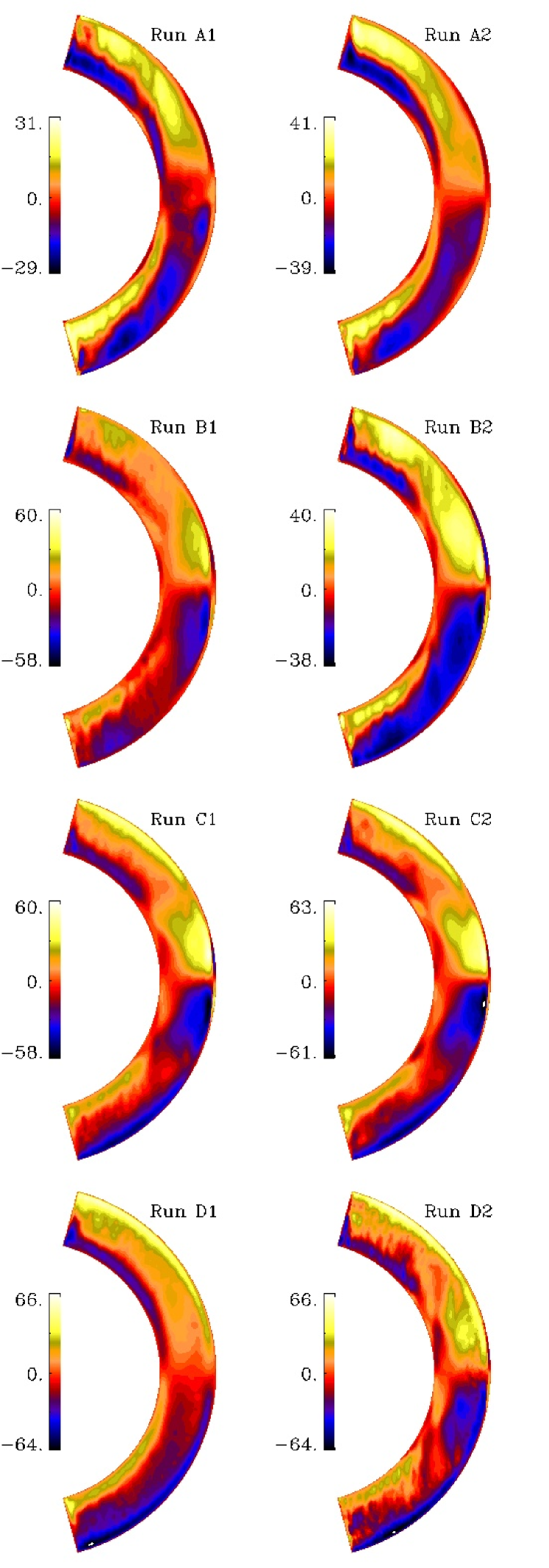
Figure 11.— Local dynamo parameter $c_{\alpha}$ from Sets A, B, C, and D.

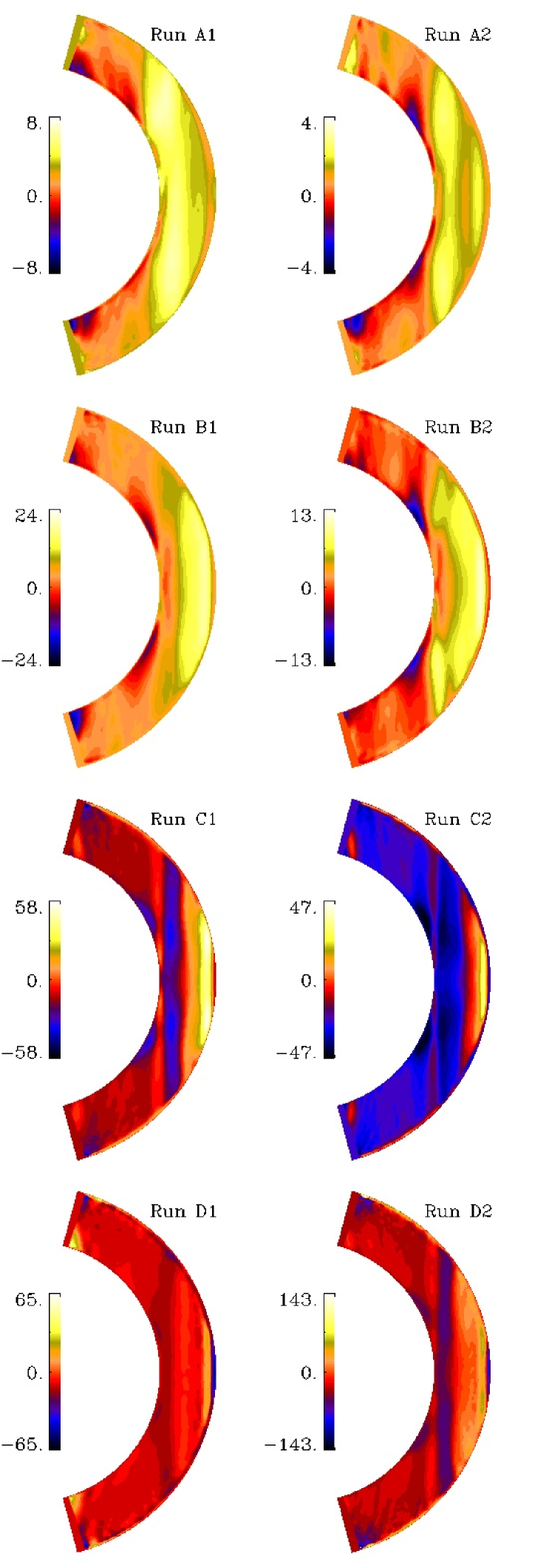
Figure 12.— Local dynamo parameter $c_{\Omega}$ from Sets A, B, C, and D. We omit regions closer to $2.5\arcdeg$ from the latitudinal boundaries.

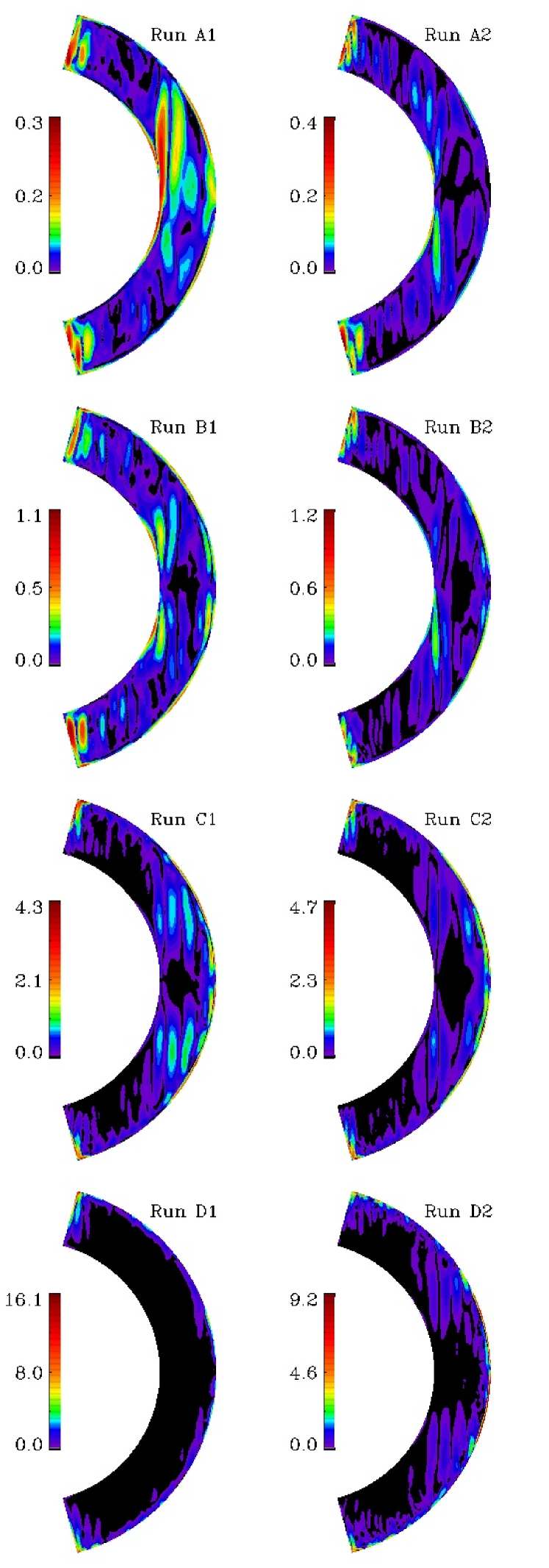
Figure 13.— Local dynamo parameter $c_{U}$ from Sets A, B, C, and D.

3.5. Estimates of local dynamo parameters

To estimate the dynamo parameters related to $\alpha$-effect, radial differential rotation, and meridional circulation, we consider local ($r$- and $\theta$-dependent) versions of dynamo numbers, referred to as local dynamo parameters that are defined by

$$c_{\alpha}=\frac{\alpha\Delta r}{\eta_{\rm t0}},\quad c_{\Omega}=\frac{\partial\overline{\Omega}/\partial r(\Delta r)^{3}}{\eta_{\rm t0}},\quad c_{U}=\frac{\overline{u}_{\rm mer}^{\rm rms}\Delta r}{\eta_{\rm t0}},$$ (35)

where $\partial\overline{\Omega}/\partial r$ is the $r$- and $\theta$-dependent radial gradient of $\overline{\Omega}$, $\Delta r=R-r_{0}$ is the thickness of the layer, and $\alpha$ is a proxy of the $\alpha$-effect (Pouquet et al., 1976),

$$\alpha=-{\textstyle{1\over 3}}\tau(\overline{\mbox{\boldmath$\omega$}\cdot{\bm{u}}}-\overline{{\bm{j}}\cdot{\bm{b}}}/\overline{\rho}),$$ (36)

with $\tau=\alpha_{\rm MLT}H_{\rm P}/u_{\rm rms}(r,\theta)$ being the local convective turnover time and $\alpha_{\rm MLT}$ the mixing length parameter. We use $\alpha_{\rm MLT}=5/3$ in this work. We estimate the turbulent diffusivity by $\eta_{\rm t0}=\tau u_{\rm rms}^{2}(r,\theta)/3$. Furthermore, $\overline{u}_{\rm mer}^{\rm rms}=\sqrt{\overline{u}_{r}^{2}+\overline{u}_{\theta}^{2}}$ is the rms value of the meridional circulation.

The results for the local dynamo parameters are shown in Figures 11–13. Generally, the values of $c_{\alpha}$ are fairly large, and those of $c_{\Omega}$ surprisingly small, suggesting that the dynamos might mainly be of $\alpha^{2}$ type. In the following, however, we focus on relative changes between different runs. It turns out that there is a weak tendency for $c_{\alpha}$ to increase as a function of $\Gamma_{\rho}$ (from Sets A to D) and ${\rm Co}$ (from subsets 1 to 2). In Set B, however, $c_{\alpha}$ decreases by a third from Run B1 to B2. The spatial distribution of $c_{\alpha}$ becomes more concentrated near the radial boundaries as $\Gamma_{\rho}$ increases.

We find that differential rotation is strongest near the equator in all cases. Sets A and B have extended regions outside the inner tangent cylinder and at low latitudes where $c_{\Omega}$ is large, but in all cases $c_{\Omega}$ is clearly smaller than $c_{\alpha}$. This is surprising given the fact that the energy of the mean toroidal field is greater than that of the mean poloidal field by a significant factor (see $E_{\rm pol}$ and $E_{\rm tor}$ in Table 2) which would be expected if differential rotation dominates over the $\alpha$-effect in maintaining the field. In Runs C1, C2, and D1, $c_{\alpha}$ and $c_{\Omega}$ have comparable magnitudes whereas in Run D2 the maximum of $c_{\Omega}$ is roughly twice that of $c_{\alpha}$. However, in these cases the toroidal and poloidal field energies are roughly comparable (see Table 2). For Set C (and especially for Run C2) there are broad regions where $c_{\Omega}$ is negative. In this connection we recall that in the diagnostic diagrams (Figure 8), C2 appears as an outlier and far away from the ${\cal A?}$ and ${\cal I?}$ branches. Furthermore, in the more strongly stratified models, $c_{\alpha}$ shows enhanced values at low latitudes. However, for the most strongly stratified models this is only true of Run D2, which is rotating slightly faster than Run D1. This is interesting in view of the fact that many mean-field dynamos produce too strong fields at high latitudes, which is then ‘artificially’ reduced by an ad-hoc factor proportional to $\sin^{2}\theta$ (Rüdiger & Brandenburg, 1995) or other such variants (Dikpati et al., 2004; Pipin & Kosovichev, 2011) for $\alpha$. We note that in local convection simulations, the $\alpha$-effect has been found to peak at mid-latitudes for rapid rotation (Käpylä et al., 2006a).

We find that $c_{U}$ is always small in comparison to both $c_{\alpha}$ and $c_{\Omega}$. Note, however, that the range of $c_{U}$ does increase as we go from Set A to Set D. Figure 13 also shows the concentration of coherent meridional circulation cells in the equatorial regions with a multi-cell structure.

In flux transport dynamos, $c_{U}$ has values of several hundreds (Küker et al., 2001). This is a consequence of choosing a small value of the turbulent magnetic diffusivity. In our simulations, on the other hand, $c_{U}$ is much smaller. This is a consequence of faster turbulent motions, making the turbulent diffusivity large and therefore $c_{U}$ small. Whether or not this also applies to more realistic models remains to be seen.

3.6. Phase relation and nature of the dynamo

The relative magnitudes of the estimated values of $c_{\alpha}$ and $c_{\Omega}$, and also the comparable amplitudes of $\overline{B}_{r}$ and $\overline{B}_{\phi}$, shown in Figure 4(a) of Käpylä et al. (2012), strongly suggest that the dynamos of this study are not of $\alpha^{2}\Omega$ type, as is usually expected for the Sun. This can be motivated further through direct inspection of the $\Omega$ term in the equation for the mean toroidal field. Following Schrinner et al. (2012), we compare the $\Omega$-effect, $r\sin\theta\overline{\bm{B}}_{\rm pol}\cdot\bm{\nabla}\overline{\Omega}$, with the mean toroidal field. The results for Runs C1 and D1 are shown in Figure 14, where we have scaled the $\Omega$ term by the magnetic cycle period, $T_{\rm cyc}$. A fraction of this would be responsible for the production of mean toroidal field for the next cycle. For Run C1, the magnitude of this term is actually large compared with $\overline{B}_{\phi}$, and the two are clearly correlated at latitudes below $\pm 35\arcdeg$, which is also where equatorward migration is seen. For Run D1, however, no clear correlation is seen even at low latitudes. The possibility of $\alpha^{2}\Omega$ type dynamo action therefore remains unclear, and especially for Run D1 it may not be the dominant mechanism. To explore the possibility that our dynamo is of $\alpha^{2}$ type, we now consider the phase relation between $\overline{B}_{r}$ and $\overline{B}_{\phi}$; see Figure 15.

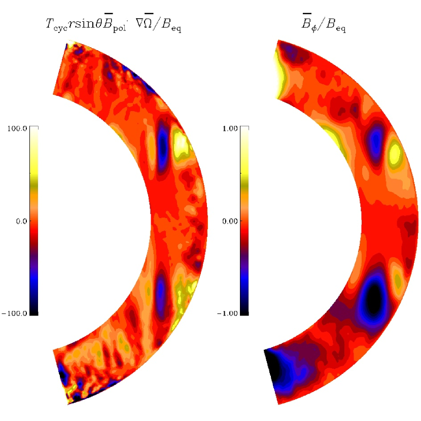
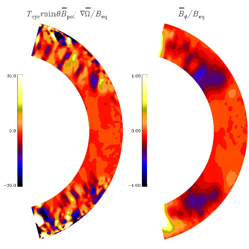
Figure 14.— $\Omega$-effect, as quantified by $T_{\rm cyc}r\sin\theta\overline{\bm{B}}_{\rm pol}\cdot\bm{\nabla}\overline{\Omega}$, where $\overline{\bm{B}}_{\rm pol}=(\overline{B}_{r},\overline{B}_{\theta})$ (left panels), and the mean toroidal magnetic field $\overline{B}_{\phi}$ (right panels) normalized by $B_{\rm eq}$ from the saturated states of Runs C1 (upper panels) and D1 (lower panel). The data is averaged over the longitude and approximately 60 convective turnover times in both cases.

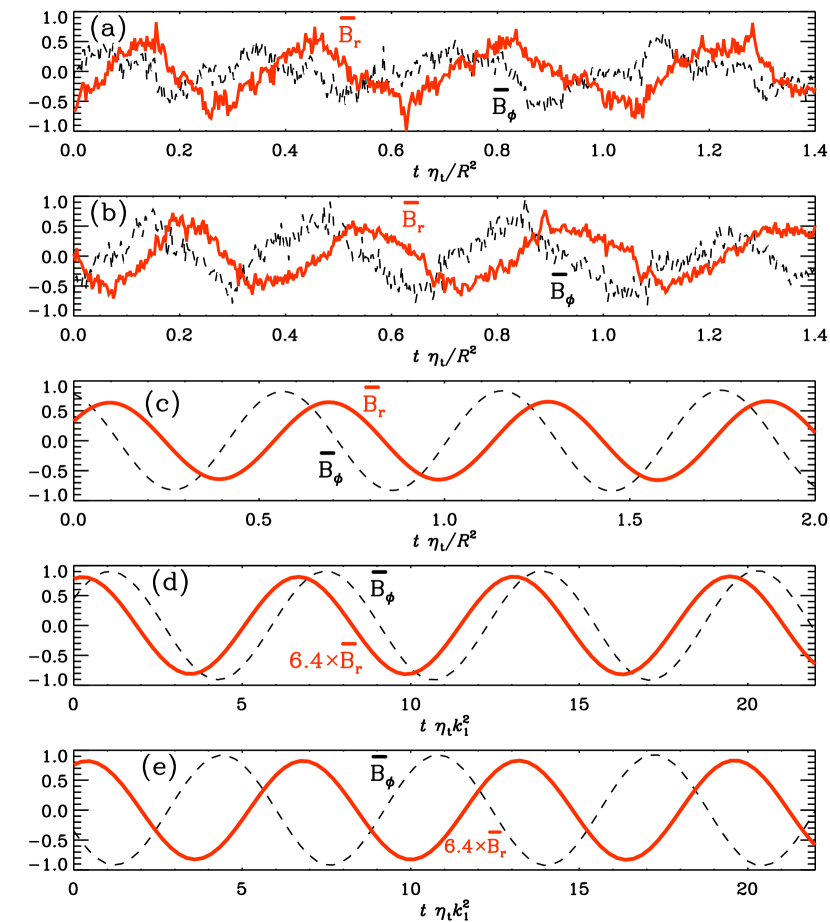
Figure 15.— Phase relations of $\overline{B}_{r}$ (thick red lines) and $\overline{B}_{\phi}$ (black dashed lines) for Run C1 at (a) $70^{\circ}$ and (b) $30^{\circ}$ latitude, compared with results of mean-field dynamos of (c) $\alpha^{2}$ type and (d), (e) $\alpha^{2}\Omega$ type, with positive and negative shear, respectively. The amplitudes have been rescaled to unity. Note that only the $\alpha^{2}$ dynamo has approximately the phase relation seen in the simulations.

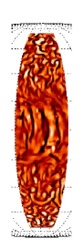
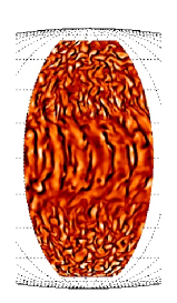
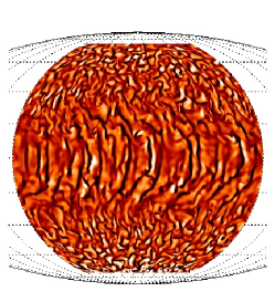
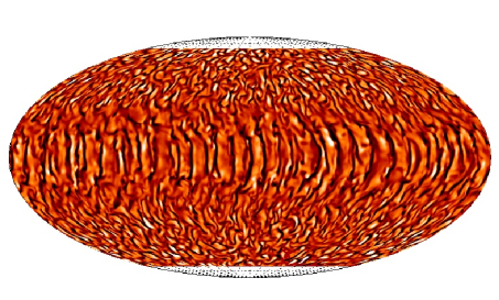
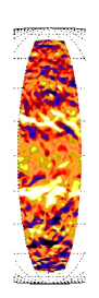
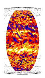
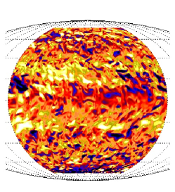
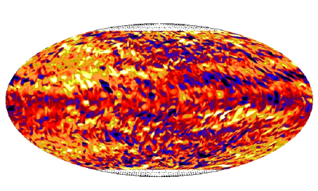
Figure 16.— Radial velocity $u_{r}$ (top row) and azimuthal magnetic field $B_{\phi}$ (bottom) near the surface of the star $r=0.98\,R$ in Mollweide projection from Runs E1 (left), E2, E3, and E4 (right). See http://youtu.be/u55sAtN2Fqs for an animation of the magnetic field in Run E4.

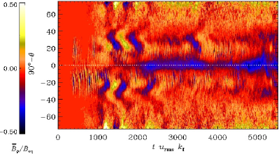
Figure 17.— Same as Figure 4 but for Run E4.

For $\alpha^{2}\Omega$ dynamos, the phase relation between $\overline{B}_{r}$ and $\overline{B}_{\phi}$ is commonly used to determine the sign of the radial differential rotation (Stix, 1976; Yoshimura, 1976). By contrast, the sign of $\alpha$ is determined by the sense of migration of the dynamo wave. For negative radial shear, $\overline{B}_{r}$ and $\overline{B}_{\phi}$ are approximately in antiphase with $\overline{B}_{\phi}$ preceding $\overline{B}_{r}$ by $\approx 3\pi/4$. For positive radial shear, $\overline{B}_{r}$ and $\overline{B}_{\phi}$ are approximately in phase with $\overline{B}_{\phi}$ lagging $\overline{B}_{r}$ by $\approx\pi/4$. In our simulations, radial shear is indeed positive, but $\overline{B}_{\phi}$ precedes $\overline{B}_{r}$ by a certain amount; see Figures 15(a) and (b). This cannot be explained by an $\alpha^{2}\Omega$ dynamo where (for positive radial shear) $\overline{B}_{\phi}$ lags $\overline{B}_{r}$ by $\pi/4$.

Another possibility are oscillatory $\alpha^{2}$ dynamos of the type recently found by Mitra et al. (2010) using direct numerical simulations of forced turbulence in a spherical wedge. Those models have also been used to study the effects of an outer coronal layer to shed magnetic helicity (Warnecke et al., 2011). Oscillatory $\alpha^{2}$ dynamos were first studied by Baryshnikova & Shukurov (1987) and Rädler & Bräuer (1987); see also the monograph of Rüdiger & Hollerbach (2004). Such solutions have also been studied in connection with the geodynamo, where the $\alpha$-effect might change sign in the middle of the outer liquid iron core (Stefani & Gerbeth, 2003). By contrast, in the simulations of Mitra et al. (2010) and Warnecke et al. (2011), $\alpha$ changes sign about the equator. They used a perfect conductor boundary condition at high latitudes and found equatorward migrating dynamo waves. With a vacuum condition, on the other hand, mean-field simulations have predicted poleward migration (Brandenburg et al., 2009). Those simulations were done in Cartesian geometry, where $(x,y,z)$ can be identified with $(r,\phi,-\theta)$. Looking at their Figure 2, it is clear that $\overline{B}_{y}$ lags $\overline{B}_{x}$ by $\pi/2$.

We have verified the phase relations of the Cartesian model of Brandenburg et al. (2009) with a one-dimensional spherical model, where $\alpha=\alpha_{0}\cos\theta$ has been assumed, which changes sign about the equator at $\theta=\pi/2$. The dynamo number for the marginally excited case is $\alpha_{0}R/\eta_{\rm t0}\approx 23.63$ and, as expected, $\overline{B}_{\phi}$ lags $\overline{B}_{r}$ by $\pi/2$; see Figure 15(c). The amplitudes have been rescaled to unity. The corresponding behavior for an $\alpha^{2}\Omega$ dynamo is shown in Figures 15(d) and (e), where $\overline{B}_{\phi}$ either precedes $\overline{B}_{r}$ by $\pi/4$ or lags $\overline{B}_{r}$ by $3\pi/4$. In this case, we have used a Cartesian model with constant $\alpha$, constant shear, $S=du_{y}/dx={\rm const}$, and periodic boundaries in a domain $0<z<L$, where the critical dynamo number is $\alpha SL^{3}/\eta_{\rm t0}^{2}\approx 8\pi^{2}$. In this model, the Cartesian coordinates $(x,y,z)$ correspond to $(-r,\phi,\theta)$, so positive (negative) values of $S$ correspond to negative (positive) radial angular velocity gradients. Neither of the phase relations of these two models agrees with those of the DNS.

Another hint pointing toward an $\alpha^{2}$ dynamo in Run C1 is, that the magnetic field is particularly strong in the middle of the convection zone ($0.8\,R<r<0.9\,R$), from where dynamo waves seem to propagate toward the surface and the bottom of the convection zone; see Figure 3(a) of Käpylä et al. (2012). Even though there exists no tachocline at the bottom or a near-surface shear layer at the top of our convection zone, the $\Omega$-effect appears to be larger toward the bottom and top of the convection zone; see Figure 12. Therefore, an $\Omega$-effect would produce the magnetic field mainly at the bottom and the top of the convection zone, which is not the case in our simulation. The case of Run D1 is more clear because the $\Omega$-effect is weak except near the boundaries (Figure 12) and the toroidal field shows no correlation with it; see Figure 14. We therefore suggest that oscillatory $\alpha^{2}$ dynamos of the type found by Mitra et al. (2010) might explain the origin of equatorward migrating dynamo waves in the spherical wedge simulations of Käpylä et al. (2012). It is also possible that this mechanism explains the poleward migration at high latitudes, but detailed comparisons must await a proper determination of $\alpha$-effect and turbulent diffusivity tensors. A first step toward this has recently been attempted by Racine et al. (2011) who estimated the tensor components of $\alpha$ by correlating the electromotive force with the mean magnetic field using singular value decomposition. These results were applied in mean-field models of Simard et al. (2013), in an effort to explain the dynamos seen by Ghizaru et al. (2010). However, this analysis is flawed in the sense that the diffusive part of the electromotive force cannot be separated from the one related to the $\alpha$-effect. This has been shown to lead to erroneous estimates of $\alpha$ (Käpylä et al., 2010a). The only reliable way to compute the turbulent diffusion tensor is currently possible with the test-field method (Schrinner et al., 2005, 2007). We postpone such analysis to a future publication.

3.7. Effect of domain size

We recently reported equatorward migration of activity belts in a spherical wedge simulation (Käpylä et al., 2012). There we gave results from simulations with a $\phi$-extent of $\pi/2$. However, at large values of the Coriolis number, the $\alpha$-effect becomes sufficiently anisotropic and differential rotation weak so that non-axisymmetric solutions become possible; see Moss & Brandenburg (1995) for corresponding mean-field models with dominant $m=1$ modes in the limit of rapid rotation. To allow for such modes, we now choose a $\phi$-extent of up to $2\pi$ for the same model as in Käpylä et al. (2012). In the present case, we find that for ${\rm Co}\approx 7.8$ it is possible that non-axisymmetric dynamo modes of low azimuthal order ($m=1$ or 2) can be dominant. This was not possible in the simulations of Käpylä et al. (2012). The same applies to non-axisymmetric modes excited in hydrodynamic convection (e.g., Busse, 2002; Brown et al., 2008; Käpylä et al., 2011b; Augustson et al., 2012).

We test the robustness of the equatorward migration by performing runs with $\phi_{0}=\pi/4$, $\pi/2$, $\pi$, and $2\pi$ with otherwise similar parameters; see Table 1. We find that the same dynamo mode producing equatorward migration is ultimately excited in all of these runs. The only qualitatively different run is that with $\phi_{0}=2\pi$ where the poleward mode near the equator grows much faster than in the other cases. However, after $tu_{\rm rms}k_{\rm f}\approx 1500$ the equatorward mode takes over similarly as in the runs with a smaller $\phi_{0}$.

The velocity field shows no marked evidence of low-degree non-axisymmetric constituents, but there are indications of $m=1$ structures in the instantaneous magnetic field (Figure 16); see also http://youtu.be/u55sAtN2Fqs for an animation of the toroidal magnetic field. This is also reflected by the fraction of the axisymmetric part of the total magnetic energy; see Columns 5 and 6 of Table 2. We find that the energy of the mean toroidal field decreases monotonically when $\phi_{0}$ is increased so that there is a factor of three in $E_{\rm tor}/E_{\rm mag}$ between the extreme cases of Runs E1 and E4. The axisymmetric part still exhibits an oscillatory mode with equatorward migration in all runs in Set E. The most prominent exception is visible in Figure 17, where we show the butterfly diagram of the $m=0$ contribution for Run E4. Clearly, equatorward migratory events are now rare and superimposed on a background of small-scale, high-frequency poleward migratory field.

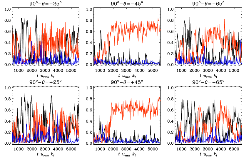
Figure 18.— Energies of the $m=0$ (black lines), 1 (red), and 2 (blue) modes of the azimuthal magnetic field as functions of time near the surface of the star ($r=0.98\,R$) in Run E4. The data is averaged over $10\arcdeg$ latitude strips centered at latitudes $90\arcdeg-\theta=\pm 25\arcdeg$ (left panels), $\pm 45\arcdeg$ (middle), and $\pm 65\arcdeg$ (right) and normalized by the total energy within each strip. The top and bottom rows refer to negative and positive latitudes, respectively.

We compute power spectra of the azimuthal component of the magnetic field from the Run E4 over three $10\arcdeg$ latitude strips from each hemisphere, centered around latitudes of $\pm 25\arcdeg$, $\pm 45\arcdeg$, and $\pm 65\arcdeg$. The results for the three lowest degrees $m=0,1,2$ are shown in Figure 18. We find that at low ($\pm 25\arcdeg$) and high ($\pm 65\arcdeg$) latitudes the axisymmetric ($m=0$) mode begins to dominate after around $1000$ turnover times and shows a cyclic pattern consistent with that seen in the time-latitude diagram of the azimuthally averaged field. After $tu_{\rm rms}k_{\rm f}\approx 1600$, however, the $m=1$ mode becomes stronger in the southern hemisphere, coinciding with the growth of the $m=1$ mode at mid-latitudes ($\pm 45\arcdeg$) where it dominates earlier in both hemispheres. This is in rough agreement with some observational results of rapid rotators, which show the most prominent non-axisymmetric temperature (e.g., Hackman et al., 2001; Korhonen et al., 2007; Lindborg et al., 2011) and magnetic structures (Kochukhov et al., 2013) at the latitudinal range around 60$\arcdeg$–80$\arcdeg$, while the equatorial and polar regions are more axisymmetric; some temperature inversions even show almost completely axisymmetric distributions in the polar regions and rings of azimuthal field at low latitudes (e.g., Donati et al., 2003). The strength of the axisymmetric versus the non-axisymmetric part in such objects has also been reported to vary over time with a time scale of a few years (Kochukhov et al., 2013).

3.8. Irradiance variations

In contrast to the constant temperature condition used earlier, the black body boundary condition (13) allows the temperature to vary at the surface of the star and thus enables the study of irradiance variations due to the magnetic cycle (Spruit, 2000). Such variations might even be responsible for driving torsional oscillations in the Sun (Spruit, 2003; Rempel, 2006). In Figure 19 we compare time–latitude surface representations ($r=R$) of azimuthally averaged temperature variations relative to its temporal average, $\Delta\overline{T}(\theta,t)=\overline{T}(\theta,t)-\langle\overline{T}\rangle_{t}(\theta)$, with those of the azimuthally averaged radial magnetic field, $\overline{B}_{r}(\theta,t)$, for Run C1 in the saturated state of the dynamo. We also show scatter plots of $\Delta\overline{T}/\overline{T}$ versus $\overline{B}_{r}/B_{\rm eq}$ at $\pm 70^{\circ}$ and $\pm 30^{\circ}$ latitude to demonstrate that there are many instances where enhanced surface magnetic activity leads to a local decrease in surface temperature. We see that

$$\Delta\overline{T}/\overline{T}\approx-Q_{T}\overline{B}_{r}^{2}/B_{\rm eq}^{2}$$ (37)

with ‘quenching’ coefficients $Q_{T}$ of $\approx 0.14$ at high latitudes and $\approx 0.33$ at low latitudes. However, there is also considerable scatter, even though our data is already longitudinally averaged. Without such averaging, the correlation between individual structures on the surface would be rather poor. The temperature modulation is best seen near the poles; see Figure 19. This could be a consequence of a strong radial magnetic field that builds up some 50–100 turnover times earlier and thus precedes the temperature signal. A weaker modulation is also seen near the equator. The peak values of $\Delta\overline{T}/\overline{T}$ at high latitudes are 15%–20% of the surface temperature; see the last two panels of Figure 19. This is relatively large compared with earlier work using mean-field models (Brandenburg et al., 1992), which showed remarkably little relative variation of the order of $10^{-3}$ in the bulk of the convection zone and even less at the surface. This difference in the modulation amplitude is probably related to the importance of latitudinal variations that were also present in the mean-field model of Brandenburg et al. (1992) and referred to as thermal shadows (Parker, 1987a).

4. Conclusions

We have studied the effects of density stratification on the dynamo solutions found in simulations of rotating turbulent convection in spherical wedge geometry for four values of $\Gamma_{\rho}$, which is the ratio of the densities at the bottom and at the surface of the convection zone. In addition, we vary the rotation rate for each value of $\Gamma_{\rho}$. For all stratifications we find quasi-steady large-scale dynamos for lower rotation and oscillatory solutions when rotation is rapid enough. The transition from quasi-steady to oscillatory modes seems to occur at a lower ${\rm Co}$ for higher stratification. Furthermore, for low values of $\Gamma_{\rho}$ the oscillatory solutions show only poleward propagation of the activity belts whereas at higher $\Gamma_{\rho}$ an equatorward branch appears at low latitudes.

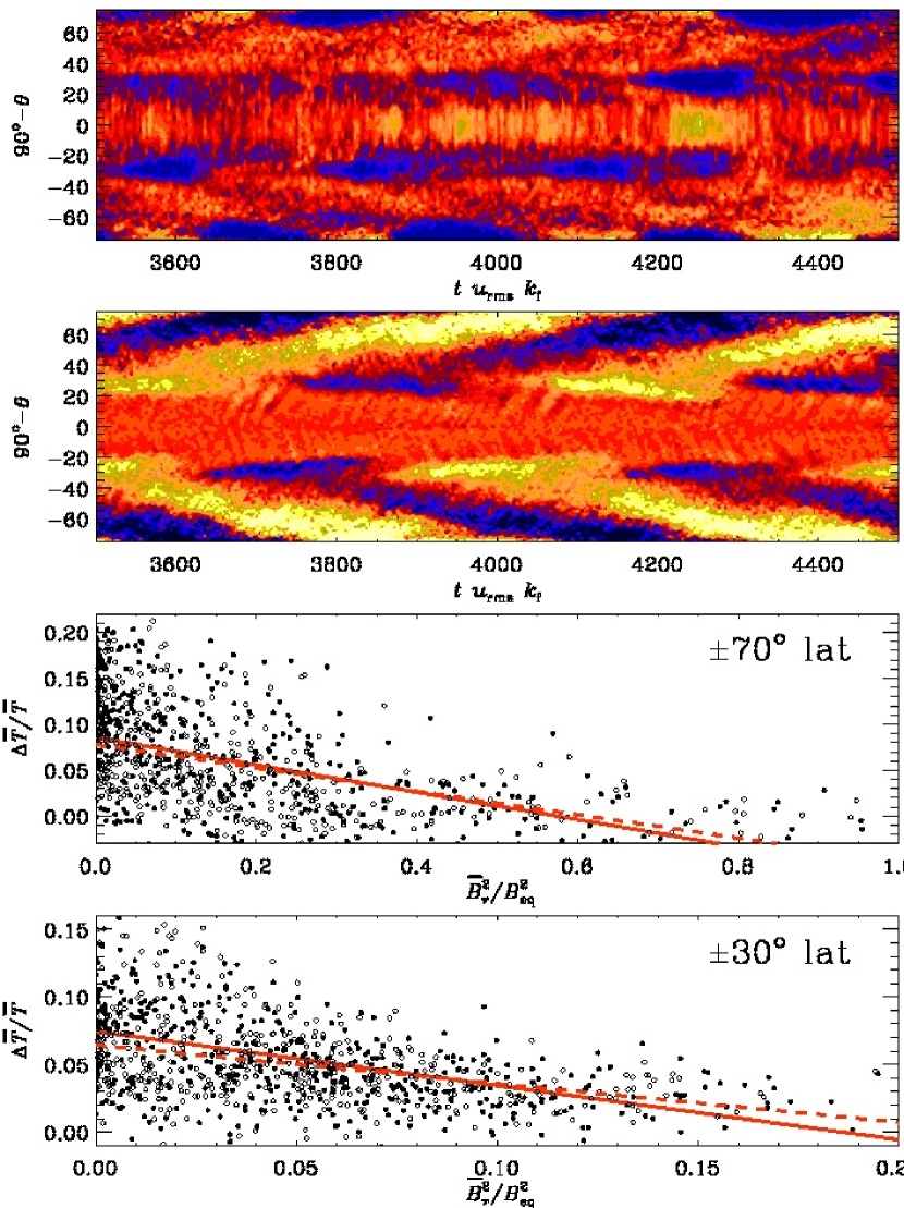
Figure 19.— Top panel: azimuthally averaged temperature fluctuations, normalized with their temporal average, $\Delta\overline{T}/\overline{T}$, at the surface as a function of time. Second panel: azimuthally averaged radial field at the surface, $\overline{B}_{r}/B_{\rm eq}$, as function of time. Lower panels: scatter plots of $\Delta\overline{T}/\overline{T}$ vs. $\overline{B}_{r}/B_{\rm eq}$ at $\pm 70^{\circ}$ and $\pm 30^{\circ}$ latitude. Here, solid (dashed) red lines and filled (open) symbols refer to northern (southern) latitudes. The slopes are $Q_{T}\approx 0.14$ and 0.33 at $\pm 70$ and $\pm 30$ latitude. All plots show quantities from the saturated stage of Run C1.

The equatorward branch was first noted by Käpylä et al. (2012) using a wedge with $\phi_{0}=90\arcdeg$ longitude extent. Here we test the robustness of this result by varying $\phi_{0}$ from $45\arcdeg$ to full $360\arcdeg$. We find a very similar pattern of the axisymmetric part of the field in all cases. However, the energy of the axisymmetric magnetic field decreases with increasing $\phi_{0}$. In the simulation with the full $\phi$-extent of $2\pi$ we observe an $m=1$ mode which is visible even by visual inspection (see Figure 16). Such field configurations have been observed in rapidly rotating late-type stars (see e.g., Kochukhov et al., 2013) and our simulation is one of the first to reproduce such features (see also Goudard & Dormy, 2008; Gastine et al., 2012). We are currently investigating the rapid rotation regime with more targeted runs which will be reported in a separate publication (Cole et al., 2013).

The ratio between cycle to rotation frequency, $\omega_{\rm cyc}/\Omega_{0}$, is argued to be an important non-dimensional output parameter of a cyclic dynamo. For the Sun and other relatively inactive stars, this ratio is around 0.01, while for the more active stars it is around 0.002. For our models we find values in the range 0.002–0.01, but for most of the runs it is around 0.004. Although it is premature to make detailed comparisons with other stars and even the Sun, it is important to emphasize that kinematic mean-field dynamos produce the correct cycle frequency only for values of the turbulent magnetic diffusivity that are at least 10 times smaller than what is suggested by standard estimates (Choudhuri, 1990). In our case, these longer cycle periods (or smaller cycle frequencies) might be a result of nonlinearity as they are only obtained in the saturated regime of the dynamo. The detailed reason for this is unclear, but it has been speculated that it is connected with a slow magnetic helicity evolution (Brandenburg, 2005). On the other hand, magnetic helicity effects are expected to become important only at values of ${\rm Rm}$ between 100 and 1000 (Del Sordo et al., 2013), which is much larger than what has been reached in the present work. Equally unclear is the reason for equatorward migration, which, as we have seen, might be a consequence of nonlinearity, as well. It will therefore be important to provide an accurate determination of all the relevant turbulent transport coefficients. The explanation favored in the present paper is that the dynamo wave is that expected for an oscillatory $\alpha^{2}$ dynamo caused by the change of sign of $\alpha$ about the equator. This is evidenced by our finding that $\overline{B}_{\phi}$ lags $\overline{B}_{r}$ by about $\pi/2$, which cannot be explained by an $\alpha^{2}\Omega$ dynamo.

References

- Arlt et al. (2005) Arlt, R., Sule, A., & Rüdiger, G. 2005, A&A, 441, 1171
- Augustson et al. (2012) Augustson, K. C., Brown, B. P., Brun, A. S., Miesch, M. S., & Toomre, J. 2012, ApJ, 756, 169
- Babcock (1961) Babcock, H. W. 1961, ApJ, 133, 572
- Baryshnikova & Shukurov (1987) Baryshnikova, I., & Shukurov, A. 1987, AN, 308, 89
- Bonanno et al. (2002) Bonanno, A., Elstner, D., Rüdiger, G., & Belvedere, G. 2002, A&A, 390, 673
- Brandenburg (2001) Brandenburg, A. 2001, ApJ, 550, 824
- Brandenburg (2005) Brandenburg, A. 2005, ApJ, 625, 539
- Brandenburg et al. (2009) Brandenburg, A., Candelaresi, S., & Chatterjee, P. 2009, MNRAS, 398, 1414
- Brandenburg et al. (2005) Brandenburg, A., Chan, K. L., Nordlund, Å., & Stein, R. F. 2005, AN, 326, 681
- Brandenburg et al. (1992) Brandenburg, A., Moss, D., & Tuominen, I. 1992, A&A, 265, 328
- Brandenburg et al. (1998) Brandenburg, A., Saar, S. H., & Turpin, C. R. 1998, ApJ, 498, L51
- Brown et al. (2008) Brown, B. P., Browning, M. K., Brun, A. S., Miesch, M. S., & Toomre, J. 2008, ApJ, 689, 1354
- Brown et al. (2010) Brown, B. P., Browning, M. K., Brun, A. S., Miesch, M. S., & Toomre, J. 2010, ApJ, 711, 424
- Brown et al. (2011) Brown, B. P., Miesch, M. S., Browning, M. K., Brun, A. S., & Toomre, J. 2011, ApJ, 731, 69
- Brun et al. (2004) Brun, A. S., Miesch, M. S., & Toomre, J. 2004, ApJ, 614, 1073
- Brun et al. (2011) Brun, A. S., Miesch, M. S., & Toomre, J. 2011, ApJ, 742, 79
- Busse (2002) Busse, F. H. 2002, PhFl, 14, 1301
- Chatterjee et al. (2004) Chatterjee, P., Nandy, D., & Choudhuri, A. R. 2004, A&A, 427, 1019
- Choudhuri (1990) Choudhuri, A. R. 1990, ApJ, 355, 733
- Choudhuri et al. (2007) Choudhuri, A. R., Chatterjee, P., & Jiang, J. 2007, Phys. Rev. Lett., 98, 131103
- Christensen & Aubert (2006) Christensen, U. R., & Aubert, J. 2006, GeoJI, 166, 97
- Cole et al. (2013) Cole, E., Käpylä, P. J., Mantere, M. J., & Brandenburg, A. 2013, submitted to ApJL, arXiv:1309.6802
- Del Sordo et al. (2013) Del Sordo, F., Guerrero, G., & Brandenburg, A. 2013, MNRAS, 429, 1686
- Dikpati & Charbonneau (1999) Dikpati, M., & Charbonneau, P. 1999, ApJ, 518, 508
- Dikpati et al. (2004) Dikpati, M., de Toma, G., Gilman, P. A., Arge, C. N., & White, O. R. 2004, ApJ, 601, 1136
- Dikpati & Gilman (2006) Dikpati, M., & Gilman, P. A. 2006, ApJ, 649, 498
- Donati et al. (2003) Donati, J.-F., et al. 2003, MNRAS, 345, 1145
- D’Silva & Choudhuri (1993) D’Silva, S., & Choudhuri, A. R. 1993, A&A, 272, 621
- Gastine et al. (2012) Gastine, T., Duarte, L., & Wicht, J. 2012, A&A, 546, A19
- Ghizaru et al. (2010) Ghizaru, M., Charbonneau, P., & Smolarkiewicz, P. K. 2010, ApJ, 715, L133
- Gilman (1983) Gilman, P. A. 1983, ApJS, 53, 243
- Glatzmaier (1985) Glatzmaier, G. A. 1985, ApJ, 291, 300
- Glatzmaier (1987) Glatzmaier, G. A. 1987, ASSL, 137, 263
- Goudard & Dormy (2008) Goudard, L., & Dormy, E. 2008, EL, 83, 59001
- Guerrero & Käpylä (2011) Guerrero, G., & Käpylä, P. J. 2011, A&A, 533, A40
- Hackman et al. (2001) Hackman, T., Jetsu, L., & Tuominen, I. 2001, A&A, 374, 171
- Hathaway (2011) Hathaway, D. H. 2011, arXiv:1103.1561
- Jouve & Brun (2007) Jouve, L., & Brun, A. S. 2007, A&A, 474, 239
- Käpylä et al. (2009) Käpylä, P. J., Korpi, M. J., & Brandenburg, A. 2009, A&A, 500, 633
- Käpylä et al. (2010a) Käpylä, P. J., Korpi, M. J., & Brandenburg, A. 2010a, MNRAS, 402, 1458
- Käpylä et al. (2010b) Käpylä, P. J., Korpi, M. J., Brandenburg, A., Mitra, D., & Tavakol, R. 2010b, AN, 331, 73
- Käpylä et al. (2006a) Käpylä, P. J., Korpi, M. J., Ossendrijver, M., & Stix, M. 2006a, A&A, 455, 401
- Käpylä et al. (2004) Käpylä, P. J., Korpi, M. J., & Tuominen, I. 2004, A&A, 422, 793
- Käpylä et al. (2006b) Käpylä, P. J., Korpi, M. J., & Tuominen, I. 2006b, AN, 327, 884
- Käpylä et al. (2011a) Käpylä, P. J., Mantere, M. J., & Brandenburg, A. 2011a, AN, 332, 883
- Käpylä et al. (2012) Käpylä, P. J., Mantere, M. J., & Brandenburg, A. 2012, ApJ, 755, L22
- Käpylä et al. (2011b) Käpylä, P. J., Mantere, M. J., Guerrero, G., Brandenburg, A., & Chatterjee, P. 2011b, A&A, 531, A162
- Kitchatinov & Mazur (2000) Kitchatinov, L. L., & Mazur, M. V. 2000, Sol. Phys., 191, 325
- Kitchatinov & Olemskoy (2012) Kitchatinov, L. L., & Olemskoy, S. V. 2012, Sol. Phys., 276, 3
- Kitchatinov et al. (1994) Kitchatinov, L. L., Pipin, V. V., & Rüdiger, G. 1994, Astron. Nachr., 315, 157
- Kitchatinov & Rüdiger (1995) Kitchatinov, L. L., & Rüdiger, G. 1995, A&A, 299, 446
- Kochukhov et al. (2013) Kochukhov, O., Mantere, M. J., Hackman, T., & Ilyin, I. 2013, A&A, 550, A84
- Korhonen et al. (2007) Korhonen, H., Berdyugina, S. V., Hackman, T., Ilyin, I. V., Strassmeier, K. G., & Tuominen, I. 2007, A&A, 476, 881
- Krause & Rädler (1980) Krause, F., & Rädler, K.-H. 1980, Mean-field Magnetohydrodynamics and Dynamo Theory (Oxford: Pergamon Press)
- Küker et al. (2001) Küker, M., Rüdiger, G., & Schultz, M. 2001, A&A, 374, 301
- Leighton (1969) Leighton, R. B. 1969, ApJ, 156, 1
- Lindborg et al. (2011) Lindborg, M., Korpi, M. J., Hackman, T., Tuominen, I., Ilyin, I., & Piskunov, N. 2011, A&A, 526, A44
- Malkus & Proctor (1975) Malkus, W. V. R., & Proctor, M. R. E. 1975, JFM, 67, 417
- Miesch et al. (2006) Miesch, M. S., Brun, A. S., & Toomre, J. 2006, ApJ, 641, 618
- Miesch et al. (2000) Miesch, M. S., Elliott, J. R., Toomre, J., Clune, T. L., Glatzmaier, G. A., & Gilman, P. A. 2000, ApJ, 532, 593
- Miesch et al. (2012) Miesch, M. S., Featherstone, N. A., Rempel, M., & Trampedach, R. 2012, ApJ, 757, 128
- Mitra et al. (2009) Mitra, D., Tavakol, R., Brandenburg, A., & Moss, D. 2009, ApJ, 697, 923
- Mitra et al. (2010) Mitra, D., Tavakol, R., Käpylä, P. J., & Brandenburg, A. 2010, ApJ, 719, L1
- Moss & Brandenburg (1995) Moss, D., & Brandenburg, A. 1995, GApFD, 80, 229
- Nelson et al. (2013) Nelson, N. J., Brown, B. P., Brun, A. S., Miesch, M. S., & Toomre, J. 2013, ApJ, 762, 73
- Oláh et al. (2000) Oláh, K., Kolláth, Z., & Strassmeier, K. G. 2000, A&A, 356, 643
- Ossendrijver (2003) Ossendrijver, M. 2003, A&A Rev., 11, 287
- Parker (1955a) Parker, E. N. 1955a, ApJ, 122, 293
- Parker (1955b) Parker, E. N. 1955b, ApJ, 121, 491
- Parker (1987a) Parker, E. N. 1987a, ApJ, 321, 984
- Parker (1987b) Parker, E. N. 1987b, Sol. Phys., 110, 11
- Pipin (2013) Pipin, V. V. 2013, in IAU Symposium, Vol. 294, IAU Symposium, ed. A. G. Kosovichev, E. de Gouveia Dal Pino, & Y. Yan, 375–386
- Pipin & Kosovichev (2011) Pipin, V. V., & Kosovichev, A. G. 2011, ApJ, 727, L45
- Pipin & Seehafer (2009) Pipin, V. V., & Seehafer, N. 2009, A&A, 493, 819
- Pouquet et al. (1976) Pouquet, A., Frisch, U., & Léorat, J. 1976, JFM, 77, 321
- Racine et al. (2011) Racine, É., Charbonneau, P., Ghizaru, M., Bouchat, A., & Smolarkiewicz, P. K. 2011, ApJ, 735, 46
- Rädler & Bräuer (1987) Rädler, K.-H., & Bräuer, H.-J. 1987, AN, 308, 101
- Rempel (2005) Rempel, M. 2005, ApJ, 622, 1320
- Rempel (2006) Rempel, M. 2006, ApJ, 647, 662
- Robinson & Chan (2001) Robinson, F. J., & Chan, K. L. 2001, MNRAS, 321, 723
- Rüdiger (1989) Rüdiger, G. 1989, Differential Rotation and Stellar Convection. Sun and Solar-type Stars (Berlin: Akademie Verlag)
- Rüdiger & Brandenburg (1995) Rüdiger, G., & Brandenburg, A. 1995, A&A, 296, 557
- Rüdiger & Hollerbach (2004) Rüdiger, G., & Hollerbach, R. 2004, The Magnetic Universe: Geophysical and Astrophysical Dynamo Theory (Weinheim: Wiley-VCH)
- Saar & Brandenburg (1999) Saar, S. H., & Brandenburg, A. 1999, ApJ, 524, 295
- Schou et al. (1998) Schou, J., et al. 1998, ApJ, 505, 390
- Schrinner et al. (2012) Schrinner, M., Petitdemange, L., & Dormy, E. 2012, ApJ, 752, 121
- Schrinner et al. (2005) Schrinner, M., Rädler, K.-H., Schmitt, D., Rheinhardt, M., & Christensen, U. 2005, AN, 326, 245
- Schrinner et al. (2007) Schrinner, M., Rädler, K.-H., Schmitt, D., Rheinhardt, M., & Christensen, U. R. 2007, GApFD, 101, 81
- Simard et al. (2013) Simard, C., Charbonneau, P., & Bouchat, A. 2013, ApJ, 768, 16
- Spruit (2000) Spruit, H. C. 2000, Space Sci. Rev., 94, 113
- Spruit (2003) Spruit, H. C. 2003, Sol. Phys., 213, 1
- Stefani & Gerbeth (2003) Stefani, F., & Gerbeth, G. 2003, Phys. Rev. E, 67, 027302
- Stix (1976) Stix, M. 1976, A&A, 47, 243
- Tobias (1998) Tobias, S. M. 1998, MNRAS, 296, 653
- Warnecke et al. (2011) Warnecke, J., Brandenburg, A., & Mitra, D. 2011, A&A, 534, A11
- Warnecke et al. (2012) Warnecke, J., Käpylä, P. J., Mantere, M. J., & Brandenburg, A. 2012, Sol. Phys., 280, 299
- Warnecke et al. (2013) Warnecke, J., Käpylä, P. J., Mantere, M. J., & Brandenburg, A. 2013, ApJ, 778, 141
- Yoshimura (1976) Yoshimura, H. 1976, Sol. Phys., 50, 3
- Zhao et al. (2013) Zhao, J., Bogart, R. S., Kosovichev, A. G., Duvall, Jr., T. L., & Hartlep, T. 2013, ApJ, 774, L29