Relativistic Lattice Boltzmann Model with Improved Dissipation

Abstract

We develop a relativistic lattice Boltzmann (LB) model, providing a more accurate description of dissipative phenomena in relativistic hydrodynamics than previously available with existing LB schemes. The procedure applies to the ultra-relativistic regime, in which the kinetic energy (temperature) far exceeds the rest mass energy, although the extension to massive particles and/or low temperatures is conceptually straightforward. In order to improve the description of dissipative effects, the Maxwell-Jüttner distribution is expanded in a basis of orthonormal polynomials, so as to correctly recover the third order moment of the distribution function. In addition, a time dilatation is also applied, in order to preserve the compatibility of the scheme with a cartesian cubic lattice. To the purpose of comparing the present LB model with previous ones, the time transformation is also applied to a lattice model which recovers terms up to second order, namely up to energy-momentum tensor. The approach is validated through quantitative comparison between the second and third order schemes with BAMPS (the solution of the full relativistic Boltzmann equation), for moderately high viscosity and velocities, and also with previous LB models in the literature. Excellent agreement with BAMPS and more accurate results than previous relativistic lattice Boltzmann models are reported.

I Introduction

Relativistic hydrodynamics and kinetic theory play a major role in many forefronts of modern physics, from large-scale applications in astrophysics and cosmology, to microscale electron flows in graphene Novoselov et al. (2004, 2005); Müller et al. (2009), all the way down to quark-gluon plasmas Shuryak (2004); Kovtun et al. (2005); Policastro et al. (2001). Due to their strong non-linearity and, for the case of kinetic theory, high dimensionality as well, the corresponding equations are extremely challenging even for the most powerful numerical methods, let alone analytics. Recently, a promising approach, based on a minimal form of relativistic Boltzmann equation, whose dynamics takes place in a fully discrete phase-space and time lattice, known as relativistic lattice Boltzmann (RLB), has been proposed by Mendoza et al. Mendoza et al. (2010a, b); Benzi et al. (1992). To date, the RLB has been applied to the simulation of weakly and moderately relativistic fluid dynamics, with Lorentz factors of $\gamma\sim 1.4$, where $\gamma=1/\sqrt{1-v^{2}/c^{2}}$, $c$ being the speed of light and $v$ the speed of the fluid. This model reproduces correctly shock waves in quark-gluon plasmas, showing excellent agreement with the solution of the full Boltzmann equation as obtained by Bouras et al. using BAMPS (Boltzmann Approach Multi-Parton Scattering) Xu and Greiner (2005); Bouras et al. (2009). The RLB makes use of two distribution functions, the first one modeling the conservation of number of particles, and the second one, the momentum-energy conservation equation. The model was constructed by matching the first and second order moments of the discrete-velocity distribution function to those of the continuum equilibrium distribution of a relativistic gas

In a subsequent work, Hupp et al.Hupp et al. (2011) improved the scheme by extending the equilibrium distribution function for the number of particles, in such a way as to include second order terms in the velocity of the fluid, thereby taming numerical instabilities for higher pressure gradients and velocities. However, the model was not able to reproduce the right velocity and pressure profiles for the Riemann problem in quark-gluon plasmas, for the case of large values of the ratio between the shear viscosity and entropy density, $\eta/s\sim 0.5$, at moderate fluid speeds ($v/c\sim 0.6$).

In order to set up a theoretical background for the lattice version of the relativistic Boltzmann equation, Romatschke et al. Romatschke et al. (2011) developed a scheme for an ultrarelativistic gas based on the expansion on orthogonal polynomials of the Maxwell-Jüttner distribution Cercignani and Kremer (2002) and, by following a Gauss-type quadrature procedure, the discrete version of the distribution and the weighting functions was calculated. This procedure was similar to the one used for the non-relativistic lattice Boltzmann model He and Luo (1997); Martys et al. (1998). This relativistic model showed very good agreement with theoretical data, although it was not compatible with a lattice, thereby requiring linear interpolation in the free-streaming step. This implies the loss of some key properties of the standard lattice Boltzmann method, such as negative numerical diffusion and exact streaming.

Very recently, Li et al. Li et al. (2012) noticed that the equation of conservation for the number of particles, recovered by the RLB model Mendoza et al. (2010a, b), exhibits incorrect diffusive effects. Therefore, they proposed an improved version of RLB, using a multi-relaxation time collision operator in the Boltzmann equation, showing that this fixes the issue with the equation for the conservation of the number of particles. The generalized collision operator allows to tune independently the bulk and shear viscosities, yielding results for the Riemann problem closer to BAMPS Xu and Greiner (2005) when the bulk viscosity is decreased. However, the third order moment of the equilibrium distribution still does not match its continuum counterpart and therefore the model still has problems to reproduce high $\eta/s\sim 0.5$, for moderately high velocities, $\beta=v/c=0.6$. Thus, while surely providing an improvement on the original RLB model, the work Li et al. (2012) did not succeed in reproducing the vanishing bulk viscosity, which is pertinent to the ultra-relativistic gas, while allowing the bulk viscosity to vary independently on the shear viscosity.

Note that in the much more studied case of the lattice Boltzmann models for the non-relativistic fluids, the question of the choice of the lattice with higher-order symmetry requirements has only recently been solved, in the framework of the entropy-compliant constriction Chikatamarla and Karlin (2006, 2009). However, the lattices (space-filling discrete-velocity sets) found in that case are tailored to reproduce the moments of the non-relativistic Maxwell-Boltzmann distribution, and do not seem to be directly transferable to the present case of the relativistic (Maxwell-Jüttner) equilibrium distribution, which has fairly different symmetries as compared to the non-relativistic Maxwell-Boltzmann distribution. Therefore, the extension of the previous LB models has to be considered anew.

In this paper, we develop a new lattice Boltzmann model capable of reproducing the third order moment of the continuum equilibrium distribution, and still realizable on a cubic lattice. The model is based on a single distribution function and satisfies conservation of both number of particles and momentum-energy equations. The model is based on the single relaxation time collision operator proposed by Anderson and Witting Anderson and Witting (1974); Cercignani and Kremer (2002) which is more appropriate for the ultra-relativistic regime than the Marle model used in the previous works, Thus, the proposed model offers significant improvement on previous relativistic lattice Boltzmann models in two respects: (i) It captures the symmetry of the higher-order equilibrium moments sufficiently to reproduce the dissipative relativistic hydrodynamics at the level of the Grad approximation to the relativistic Boltzmann equation; (ii) It represents a genuine lattice Boltzmann discretization of space and time, with no need of any interpolation scheme, thereby avoiding the otherwise ubiquitous spurious dissipation. The new lattice Boltzmann model is shown to reproduce with very good accuracy the results of the shock-waves in quark-gluon plasmas, for moderately high velocities and high ratios $\eta/s$.

The paper is organized as follows: in Sec. II we describe in detail the model and the way it is constructed; in Sec. III, we implement simulations of the Riemann problem in order to validate our model and compare it with BAMPS and previous relativistic lattice Boltzmann models; finally, in Sec. IV, we discuss the results and future work.

II Model Description

II.1 Symmetries of the relativistic Boltzmann equation

To build our model, we start from the relativistic Boltzmann equation for the probability distribution function $f$:

$$p^{\mu}\partial_{\mu}f=-\frac{p_{\mu}U^{\mu}}{c^{2}\tau}(f-f^{\rm eq})\quad,$$ (1)

where the local equilibrium is given by the Maxwell-Jüttner equilibrium distribution Cercignani and Kremer (2002),

$$f^{\rm eq}=A\exp(-p^{\mu}U_{\mu}/k_{B}T)\quad,$$ (2)

In the above, $A$ is a normalization constant, $c$ the speed of light, and $k_{B}$ the Boltzmann constant. The $4$-momentum vectors are denoted by $p^{\mu}=(E/c,\vec{p})$, and the macroscopic 4-velocity by $U^{\mu}=(c,\vec{u})\gamma(u)$, with $\vec{u}$ the three-dimensional velocity of the fluid. Note that we have used the Anderson-Witting collision operatorAnderson and Witting (1974) (rhs of Eq. (1)), making our model compatible with the ultrarelativistic regime. Hereafter, we will use natural units, $c=k_{B}=1$, and work in the ultrarelativistic regime, $\xi\equiv mc^{2}/k_{B}T\ll 1$.

According to a standard procedure He and Luo (1997); Martys et al. (1998); Romatschke et al. (2011), we first expand the Maxwell-Jüttner distribution in the rest frame, $f^{\rm eq}=A\exp(-p^{0}/T)$, in an orthogonal basis. Since in the ultrarelativistic regime, $p^{0}/T=\sqrt{\vec{p}^{2}/T^{2}+m^{2}/T^{2}}\simeq p/T$, being $p=\sqrt{\vec{p}^{2}}$, we can write the equilibrium distribution in spherical coordinates,

$$\int ge^{-p_{0}/T}\frac{d^{3}p}{p^{0}}=\int_{0}^{\infty}\int_{0}^{\pi}\int_{0}^{2\pi}gpe^{-p/T}dp\sin(\theta)d\theta d\phi\quad,$$ (3)

where $g$ is an arbitrary function of momentum. Following Romatschke Romatschke et al. (2011), we can expand the distribution in each coordinate separately, and subsequently, by using a Gauss quadrature, calculate the discrete values of the 4-momentum vectors. Thus, the discrete equilibrium distribution can be written as,

$$f_{l}^{\rm eq}=\sum_{i,j,k}a_{ijk}(U^{\mu})P_{i}(\theta_{l}){\cal R}_{j}(p_{l})F_{k}(\phi_{l})\quad,$$ (4)

where the coefficients $a_{ijk}(U^{\mu})$ are the projections of the distribution on the polynomials $P_{i}(\theta_{l}){\cal R}_{j}(p_{l})F_{k}(\phi_{l})$, and the discrete 4-momenta are denoted by $p_{l}^{\mu}=(p_{l},p_{l}\cos(\phi_{l})\sin(\theta_{l}),p_{l}\sin(\phi_{l})\sin(\theta_{l}),p_{l}\cos(\theta_{l}))$. Consequently, the discrete form of the Boltzmann equation takes the form,

$$f_{l}(x^{\mu}+p_{l}^{\mu}/p_{l}^{0}\delta t,t+\delta t)-f_{l}(x^{\mu},t)=-\frac{p_{l\mu}U^{\mu}\delta t}{\tau p_{l}^{0}}(f_{l}-f_{l}^{\rm eq})\quad.$$ (5)

However, note that, in the streaming process on the right-hand-side of Eq.(5), the distribution moves at velocity $p_{l}^{\mu}/p_{l}^{0}$, which implies that the information travels (in a single time step) from each cell center to a position that belongs to the surface of a sphere of radius $c\;\delta t=1$. Furthermore, to represent correctly the third order moment of the equilibrium distribution,

$$P^{\alpha\beta\lambda}=\sum_{l}f^{\rm eq}_{l}p_{l}^{\alpha}p_{l}^{\beta}p_{l}^{\lambda}\quad,$$ (6)

the number of points needed on the surface of the unit sphere exceeds $6$ and $12$, which correspond to the first neighbors for a cubic and hexagonal closed packed (HCP) lattices, respectively. This implies that, in general, the 4-vectors $p^{\mu}/p^{0}$ cannot be embedded into a regular lattice, and therefore, an interpolation algorithm has to be used. By doing this, we are losing one of the most important features of lattice Boltzmann models, which is the exact streaming. Thus, within this spherical coordinate representation, the streaming process cannot take place on a regular lattice.

II.2 Moment projection of the equilibrium

In this work, we shall use a different approach to the quadrature representation. We first expand the equilibrium distribution at rest, $w(p^{0})=f^{\rm eq}=A\exp(-p^{0})$ by using Cartesian coordinates, unlike the spherical coordinate system used in Ref. Romatschke et al. (2011), and choose the 4-momentum vectors such that they belong to the lattice (from now on and without loss of generality, we will use the notation $p^{0}/T\rightarrow p^{0}$). This procedure also avoids extra terms in the product, $P_{i}(\theta_{l}){\cal R}_{j}(p_{l})F_{k}(\phi_{l})$ for the spherical case, which are not necessary if we only need to recover correctly the first three moments of the equilibrium distribution. This considerably simplifies the discrete equilibrium distribution.

By performing a Gram-Schmidt procedure with the weight $w(p^{0})$, we construct a set of orthonormal polynomials. The orthonormal polynomials in cartesian coordinates up to third order, herefrom denoted by $J_{k}$, where the index $k$ runs from $0$ to $29$, are shown in Table 1.

Order	Polynomial $J_{k}$	$k$
$0$th	1	0
$1$st	$\frac{p^{0}-2}{\sqrt{2}}$, $\frac{p^{x}}{\sqrt{2}}$, $\frac{p^{y}}{\sqrt{2}}$, $\frac{p^{z}}{\sqrt{2}}$	1, 2, 3, 4
$2$nd	$\frac{(p^{0}-6)p^{0}+6}{2\sqrt{3}}$, $\frac{(p^{0}-4)p^{x}}{2\sqrt{2}}$, $\frac{(p^{0}-4)p^{y}}{2\sqrt{2}}$	5, 6, 7
	$\frac{(p^{0}-4)p^{z}}{2\sqrt{2}}$, $\frac{-p^{02}+p^{x2}+2p^{y2}}{4\sqrt{2}}$, $-\frac{p^{02}-3p^{x2}}{4\sqrt{6}}$	8, 9, 10
	$\frac{p^{x}p^{z}}{2\sqrt{2}}$, $\frac{p^{y}p^{z}}{2\sqrt{2}}$, $\frac{p^{x}p^{y}}{2\sqrt{2}}$	11, 12, 13
$3$rd	$\frac{1}{12}(p^{0}-6)^{2}p^{0}-2$, $\frac{((p^{0}-10)p^{0}+20)p^{x}}{4\sqrt{5}}$	14, 15
	$-\frac{1}{24}(p^{0}-6)\left(p^{02}-3p^{x2}\right)$, $\frac{5p^{x3}-3p^{02}p^{x}}{24\sqrt{5}}$	16, 17
	$\frac{((p^{0}-10)p^{0}+20)p^{y}}{4\sqrt{5}}$, $\frac{(p^{0}-6)p^{x}p^{y}}{4\sqrt{3}}$, $\frac{p^{x}p^{y}p^{z}}{4\sqrt{3}}$	18, 19, 20
	$-\frac{(p^{0}-6)\left(p^{02}-p^{x2}-2p^{y2}\right)}{8\sqrt{3}}$, $\frac{p^{x}\left(-p^{02}+p^{x2}+2p^{y2}\right)}{8\sqrt{3}}$	21, 22
	$\frac{p^{y}\left(-3p^{02}+3p^{x2}+4p^{y2}\right)}{24\sqrt{2}}$, $\frac{((p^{0}-10)p^{0}+20)p^{z}}{4\sqrt{5}}$	23, 24
	$\frac{(p^{0}-6)p^{x}p^{z}}{4\sqrt{3}}$, $-\frac{p^{z}\left(p^{02}-5p^{x2}\right)}{8\sqrt{30}}$, $\frac{(p^{0}-6)p^{y}p^{z}}{4\sqrt{3}}$	25, 26, 27
	$\frac{(p^{0}-6)p^{y}p^{z}}{4\sqrt{3}}$, $\frac{p^{z}\left(-p^{02}+p^{x2}+4p^{y2}\right)}{24\sqrt{2}}$	28, 29

Table 1: Polynomials $J_{k}$ that are orthonormal on the weight function $w(p^{0})$ in Cartesian coordinates $(x,y,z)$.

Note that in this Table, the 4-momentum has the notation $p^{\mu}=(p^{0},p^{x},p^{y},p^{z})$. Since these polynomials are orthonormal, there are no normalization factors, and the Maxwell-Jüttner distribution can be approximated, up to third order in the momentum space, by an expansion as simple as

$$f^{\rm eq}\simeq\sum_{k=0}^{29}w(p^{0})a_{k}(T,U^{\mu})J_{k}(p^{\mu})\quad,$$ (7)

where the projections $a_{k}$ are calculated by,

$$a_{k}=\int f^{\rm eq}J_{k}(p^{\mu})\frac{d^{3}p}{p^{0}}\quad.$$ (8)

Since the Anderson-Witting model is only compatible with the Landau-Lifshitz decomposition Cercignani and Kremer (2002); Anderson and Witting (1974), we must calculate the energy density of the fluid by solving the eigenvalue problem,

$$T^{\alpha\beta}U_{\beta}=\epsilon U^{\alpha}\quad,$$ (9)

$\epsilon$ being the energy density of the fluid, and

$$T^{\alpha\beta}=\int fp^{\alpha}p^{\beta}\frac{d^{3}p}{p^{0}}\quad,$$ (10)

the momentum-energy tensor. For the particle density, we use the relation,

$$n=U_{\alpha}\int fp^{\alpha}\frac{d^{3}p}{p^{0}}\quad,$$ (11)

and, by using the equation of state, $\epsilon=3nT$, we can calculate the temperature of the fluid.

II.3 Discrete-velocity representation of the quadratures

Note that the above derivation using Cartesian coordinates still refers to the continuous 4-momenta. In order to discretize the above moment projection of the equilibrium distribution, we must choose a set of 4-momentum vectors that satisfies the very same orthonormality conditions, namely:

$$\int w(p^{0})J_{l}(p^{\mu})J_{k}(p^{\mu})\frac{d^{3}p}{p^{0}}=\sum_{i}w_{i}J_{l}(p^{\mu}_{i})J_{k}(p^{\mu}_{i})=\delta_{lk}\quad,$$ (12)

while, at the same time, $p^{\mu}/p^{0}$ corresponds to lattice points. Here, we choose to work with a cubic lattice, although the procedure described here also applies to other ones, e.g. HCP lattice.

Since, due to its nature, $p^{\mu}/p^{0}$ leads to velocity vectors which belong to a sphere of radius $c$ in the space components, using the procedure in Ref. Romatschke et al. (2011) will generally result in off-site lattice points. For this reason, we opt for another quadrature based on this orthonormality condition, and impose that the distribution function at rest frame should satisfy the moments of the equilibrium distribution, up to $6$-th order. This is made to ensure that the $5$-th order moment of the equilibrium distribution is recovered (at least at very low fluid velocities), which, in the context of the Grad theory for the Anderson-Witting model Cercignani and Kremer (2002), is a requirement for the correct calculation of the transport coefficients, namely the shear and bulk viscosities and thermal conductivity. The condition for the $6$-th order moment, is to choose from the multiple lattice solutions, the one that presents the highest symmetry to model the Maxwell-Jüttner distribution. In order to use general features of classical lattice Boltzmann models, like bounce-back boundary conditions to impose zero velocity on solid walls, we will also require that the weights $w_{i}$ corresponding to the discrete 4-momentum vectors $p_{i}^{k}$ have the same values as the ones corresponding to $-p_{i}^{k}$ (latin indices run over spatial components).

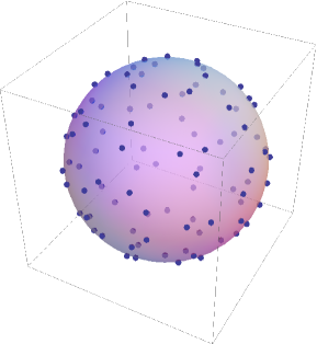
Figure 1: Directions of the velocity vectors $\vec{\vartheta}_{i}$ to recover up to the third order moment of the Maxwell-Jüttner distribution. The radius of the sphere is $R=\sqrt{41}$. The points represent lattice sites belonging to the sphere surface.

In order to generate on-site lattice points, let us first analyse the relativistic Boltzmann equation, which can be written as,

$$p^{0}\partial_{t}f+p^{a}\partial_{a}f=-\frac{p_{\mu}U^{\mu}}{\tau}(f-f^{\rm eq})\quad,$$ (13)

and in the ultrarelativistic regime,

$$p^{0}(\partial_{t}f+v^{a}\partial_{a}f)=-\frac{p_{\mu}U^{\mu}}{\tau}(f-f^{\rm eq})\quad.$$ (14)

where $v^{a}$ are the components of the microscopic velocity. These microscopic velocities have the same magnitude but, in general, different directions. Dividing both sides of Eq.(16) by $p^{0}$, we obtain

$$\partial_{t}f+v^{a}\partial_{a}f=-\frac{p_{\mu}U^{\mu}}{\tau p^{0}}(f-f^{\rm eq})\quad.$$ (15)

In other words, in the ultra-relativistic regime, the relativistic Boltzmann equation can be cast into a form where the time derivative and the propagation term become the same as in the non-relativistic case, at the price of an additional dependence on $p^{0}$ in the relaxation term. However, since this newly acquired dependence remains local, we shall be able to find a discrete-velocity quadrature which also allows for a lattice Boltzmann-type discretization in time and space without any interpolation. Indeed, in a cubic cell of length $\delta x=1$ there are only $6$ neighbors, which are not sufficient to satisfy the orthogonality conditions and the third order moment of the equilibrium distribution. However, by multiplying this equation by a constant $R$ at both sides, and performing a time transformation (dilatation), $\delta t\rightarrow R\delta t^{\prime}$ and $\tau\rightarrow R\tau^{\prime}$, we obtain

$$\partial_{t^{\prime}}f+\vartheta^{a}\partial_{a}f=-\frac{p_{\mu}U^{\mu}}{\tau^{\prime}p^{0}}(f-f^{\rm eq})\quad,$$ (16)

where we have defined $\vartheta^{a}=Rv^{a}$. Due to this transformation, the 4-momentum vectors are reconstructed through the relation

$$p^{\mu}=p^{0}(1,\vec{\vartheta}/R)\quad,$$ (17)

At this stage, we can choose the radius of the sphere such that the lattice points that belong to the surface of the sphere and the cubic lattice exhibit enough symmetries to satisfy both conditions. This is equivalent to solving the Diophantine equation,

$$n_{x}^{2}+n_{y}^{2}+n_{z}^{2}=R^{2}\quad,$$ (18)

where $n_{x}$, $n_{y}$, and $n_{z}$ are integer numbers, being $\vec{\vartheta}=(n_{x},n_{y},n_{z})$. Thus, we can determine the components of the discrete version of the velocities $\vec{\vartheta}$ which are needed for the streaming term in the Boltzmann equation, lhs of Eq. (16). However, on the rhs of this equation, and for the calculation of the discrete 4-momentum vectors via Eq. (17), we also need to know the discrete values of $p^{0}$. The 4-vector $p^{\mu}$ is needed to compute the orthonormality conditions given by Eq. (12) and the moments of the equilibrium distribution.

Due to the fact that $p^{0}$ is the magnitude of the 4-momentum, $p^{0}=\sqrt{p^{\mu}p_{\mu}}$, in $3+1$-dimensional spacetime, it is natural to assume that its discrete values can be calculated by using the weight function in spherical coordinates, $w(p)=4\pi Ap^{2}\exp(-p)$, where the angular components have been integrated out, and using the zeros of its respective orthonormal polynomial of fourth order (this is because we are interested in an expansion up to third order, so we need one more order to calculate the zeros). This fourth order polynomial is given by:

$${\cal R}^{(4)}(p)=\frac{1}{24\sqrt{5}}[120+p(-240+p[120+(p-20)p])]\quad.$$ (19)

To summarize, in order to calculate the discrete $p^{\mu}_{i}$ and their respective $w_{i}$, we first fix $R$ and solve the equations

$$n_{x}^{2}+n_{y}^{2}+n_{z}^{2}=R^{2}\quad,$$ (20a)

$${\cal R}^{(4)}(p)=0\quad,$$ (20b)

to obtain the solutions for $n_{x}$, $n_{y}$, $n_{z}$, and $p$. With these values, we build the discrete 4-vectors

$$p_{lm}^{\mu}=p_{l}^{0}(1,n_{x,m}/R,n_{y,m}/R,n_{z,m}/R)\quad,$$ (21)

where $l=1,...,4$ denotes the four zeros of the polynomial ${\cal R}^{(4)}(p)$, and $m=0,...,{\cal M}$ the triplets $(n_{x},n_{y},n_{z})_{m}$ that satisfy the Diophantine equation, assuming that ${\cal M}$ is the number of solutions. Here, for simplicity, we regroup the pair of indexes _lm to _i, so that we can label the discrete 4-momentums as $p^{\mu}_{i}$, where $i=1,...,{\cal N}$ with ${\cal N}=4\times{\cal M}$.

Next, we replace these values into the equations,

$$\int w(p^{0})J_{l}(p^{\mu})J_{k}(p^{\mu})\frac{d^{3}p}{p^{0}}=\sum_{i}^{\cal N}w_{i}J_{l}(p^{\mu}_{i})J_{k}(p^{\mu}_{i})=\delta_{lk}\quad,$$ (22a)

$$\int w(p^{0})p^{\mu}p^{\nu}p^{\sigma}p^{\lambda}\frac{d^{3}p}{p^{0}}=\sum_{i}^{\cal N}w_{i}p_{i}^{\mu}p_{i}^{\nu}p_{i}^{\sigma}p_{i}^{\lambda}\quad,$$ (22b)

$$\int w(p^{0})p^{\mu}p^{\nu}p^{\sigma}p^{\lambda}p^{\gamma}\frac{d^{3}p}{p^{0}}=\sum_{i}^{\cal N}w_{i}p_{i}^{\mu}p_{i}^{\nu}p_{i}^{\sigma}p_{i}^{\lambda}p_{i}^{\gamma}\quad,$$ (22c)

$$\int w(p^{0})p^{\mu}p^{\nu}p^{\sigma}p^{\lambda}p^{\gamma}p^{\beta}\frac{d^{3}p}{p^{0}}=\sum_{i}^{\cal N}w_{i}p_{i}^{\mu}p_{i}^{\nu}p_{i}^{\sigma}p_{i}^{\lambda}p_{i}^{\gamma}p_{i}^{\beta}\quad,$$ (22d)

$$w_{i}=w_{j}\quad\text{(if $p^{k}_{i}=-p^{k}_{j}$)}\quad,$$ (22e)

$$w_{i}\geq 0\quad,$$ (22f)

and look for any solution for $w_{i}$ that fulfills the above relations. Should none be found, we repeat the procedure with a different value of $R$. By performing this iteration process, we found that $R=\sqrt{41}$ is sufficient to recover up to the third order moment of the Maxwell-Jüttner distribution, and up to sixth order of this distribution in the Lorentz rest frame.

The corresponding discrete velocity vectors $\vec{\vartheta}_{m}$ are: $(\pm 6,\pm 2,\pm 1)$, $(\pm 6,\pm 1,\pm 2)$, $(\pm 2,\pm 6,\pm 1)$, $(\pm 1,\pm 6,\pm 2)$, $(\pm 1,\pm 2,\pm 6)$, $(\pm 2,\pm 1,\pm 6)$, $(\pm 5,0,\pm 4)$, $(\pm 5,\pm 4,0)$, $(0,\pm 5,\pm 4)$, $(\pm 4,\pm 5,0)$, $(0,\pm 4,\pm 5)$, $(\pm 4,0,\pm 5)$, $(\pm 4,\pm 3,\pm 4)$, $(\pm 3,\pm 4,\pm 4)$, and $(\pm 4,\pm 4,\pm 3)$; with the values for $p_{l}^{0}\simeq 0.743$, $2.572$, $5.731$, and $10.95$. Consequently, this gives a total of 4-momentum vectors ${\cal N}=384$. However, the last condition in Eq. (22) allows some weights to become zero. Therefore, in our iteration procedure, we have taken the minimal number of 4-momentum vectors $p^{\mu}_{i}$, by imposing the maximum number of $w_{i}$ to be zero. For this reason, there are only $128$ vectors $p^{\mu}_{i}$ needed to fulfill the conditions in Eq. (22). In principle, all the velocity vectors $\vec{\vartheta}_{m}$ are needed, but only some of the combinations with $p^{0}_{l}$ are required. The detailed list of the $\vec{\vartheta}_{m}$, $p^{0}_{l}$, and $p^{\mu}_{i}$, and their respective discrete weight functions $w_{i}$ are given in the Supplementary Material sup .

In Fig. 1 we report the configuration of the velocity vectors $\vec{\vartheta}$ to achieve the third order moment of the Maxwell-Jüttner distribution function. The points correspond to lattice nodes of a cubic lattice that, at the same time, belong to the surface of the respective sphere of radius $R=\sqrt{41}$. The relatively large number of discrete velocities should not come as a surprise; in the case of non-relativistic lattice Boltzmann, the number of discrete velocities also becomes high (at least 41 for achieving complete Galilean invariance in the non-thermal case and $125$ in the thermal case, see Chikatamarla and Karlin (2006, 2009)). Note that the specified values of $p^{0}$ play the same role in defining the quadrature as the reference temperature (energy) in the non-relativistic case Chikatamarla and Karlin (2006, 2009).

Finally, we can write the discrete version of the equilibrium distribution up to third order,

$$f_{i}^{\rm eq}=w_{i}\sum_{n=0}^{29}a_{n}(T,U^{\mu})J_{n}(p_{i}^{\mu})\quad,$$ (23)

which is shown in details in Appendix B, Eq. (44). Note that this distribution function recovers the first three moments of the Maxwell-Jüttner distribution in the ultrarelativistic regime,

$$\int f^{\rm eq}p^{\mu}\frac{d^{3}p}{p^{0}}=\sum_{i=1}^{128}f_{i}^{\rm eq}p_{i}^{\mu}=N^{\mu}\quad,$$ (24)

$$\int f^{\rm eq}p^{\mu}p^{\nu}\frac{d^{3}p}{p^{0}}=\sum_{i=1}^{128}f_{i}^{\rm eq}p_{i}^{\mu}p_{i}^{\nu}=T^{\mu\nu}\quad,$$ (25)

$$\int f^{\rm eq}p^{\mu}p^{\nu}p^{\lambda}\frac{d^{3}p}{p^{0}}=\sum_{i=1}^{128}f_{i}^{\rm eq}p_{i}^{\mu}p_{i}^{\nu}p^{\lambda}=P^{\mu\nu\lambda}\quad,$$ (26)

where

$$N^{\nu}=nU^{\nu}\quad,$$ (27)

$$T^{\nu\mu}=-nT\eta^{\nu\mu}+4nTU^{\nu}U^{\mu}\quad,$$ (28)

being the number of particles 4-flow and the energy-momentum tensor, respectively, and

$$P^{\nu\mu\lambda}=-4nT^{2}(\eta^{\nu\mu}U^{\lambda}+\eta^{\nu\lambda}U^{\mu} +\eta^{\mu\lambda}U^{\nu})$$ (29)

$$+24nT^{2}U^{\nu}U^{\mu}U^{\lambda}\quad,$$

with $n=2T^{3}$. However, the extension to the case of massive particles is straightforward, by changing the coefficients, $a_{n}$, in Eqs. (8) and (23).

II.4 Discrete relativistic Boltzmann equation

In the model of Anderson-Witting for the collision operator, the relativistic Boltzmann equation takes the form given by Eq. (1),

$$p^{\mu}\partial_{\mu}f=-\frac{p^{\mu}U_{\mu}}{\tau}(f-f^{\rm eq})\quad.$$ (30)

This collision operator is compatible with the Landau-Lifshitz decomposition Cercignani and Kremer (2002), which implies fulfillment of the following relations

$$U_{\mu}N^{\mu}=U_{\mu}\int fp^{\mu}\frac{d^{3}p}{p^{0}}=U_{\mu}N_{E}^{\mu}=\int f^{\rm eq}p^{\mu}\frac{d^{3}p}{p^{0}}\quad,$$ (31a)

$$U_{\mu}T^{\mu\nu}=U_{\mu}\int fp^{\mu}p^{\nu}\frac{d^{3}p}{p^{0}}=U_{\mu}T_{E}^{\mu\nu}=\int f^{\rm eq}p^{\mu}p^{\nu}\frac{d^{3}p}{p^{0}}\quad,$$ (31b)

Here, the subscript $E$ denotes the quantities calculated with the equilibrium distribution. Therefore, upon integrating Eq. (30) in momentum space, we obtain

$$\partial_{\mu}N^{\mu}=0\quad,$$ (32)

which is the conservation of the number of particles 4-flow. By multiplying by $p^{\nu}$ and integrating, we obtain the conservation of the momentum energy tensor

$$\partial_{\mu}T^{\mu\nu}=0\quad.$$ (33)

In order to calculate the transport coefficients, we need the third order moment, so that, upon multiplying Eq. (30) by $p^{\nu}p^{\beta}$, we obtain

$$\partial_{\mu}P^{\mu\nu\beta}=-\frac{1}{\tau}(U_{\mu}P^{\mu\nu\beta}-U_{\mu}P_{E}^{\mu\nu\beta})\quad,$$ (34)

and by using a Maxwellian iteration method Cercignani and Kremer (2002),

$$U_{\mu}P^{\mu\nu\beta}-U_{\mu}P_{E}^{\mu\nu\beta}=-\tau\partial_{\mu}P_{E}^{\mu\nu\beta}\quad.$$ (35)

Note that we need at least the third order moment of the equilibrium distribution, $P_{E}^{\mu\nu\beta}$, to compute the dissipation coefficients (namely, bulk and shear viscosities and heat conductivity). This requirement is fulfilled in our discrete and continuum expansions of the equilibrium distribution via Eqs. (24), (25), (26). However, to recover full dissipation, we would also need to recover the third moment of the non-equilibrium distribution, which according to the $14$ moments Grad’s theory , can be written as,

$$P^{\mu\nu\beta}=P_{E}^{\mu\nu\beta}+b_{\alpha}P_{E}^{\mu\nu\beta\alpha}+d_{\alpha\lambda}P_{E}^{\mu\nu\beta\alpha\lambda}\quad,$$ (36)

where $b_{\alpha}$ and $d_{\alpha\lambda}$ are coefficients that carry the information on the transport coefficients Cercignani and Kremer (2002). Note that we need to recover terms up to the fifth order of the equilibrium distribution. In principle, this could be done by the procedure described on this paper, but the resulting value for $R$ could be unpractically large. Nevertheless, at low velocities, $U^{\mu}\sim(1,0,0,0)$, the Maxwell-Jüttner distribution can be approximated by the weight function $w(p^{0})$, and in analogy to the discrete case, by $w_{i}$, and the fourth and fifth order are recovered via Eq. (22). As a result, at relatively low velocities, we expect the non-equilibrium third order tensor to be also fulfilled. Therefore, the transport coefficients for an ultrarelativistic gas, i.e. $\mu=0$ for the bulk viscosity, $\eta=(2/3)P\tau$ for the shear viscosity, and $\lambda=(4/5T)P\tau$ for the thermal conductivity, also apply to our model.

To discretize the relativistic Boltzmann equation, we first implement the time transformation described in the previous section and integrate in time Eq. (30) between $t^{\prime}$ and $t^{\prime}+\delta t^{\prime}$. This yields:

$$f(x^{a}+\vartheta^{a}\delta t^{\prime},t^{\prime}+\delta t^{\prime})-f(x^{a},t^{\prime})=-\frac{p^{\mu}U_{\mu}}{\tau^{\prime}p^{0}}(f-f^{\rm eq})\delta t^{\prime}\quad.$$ (37)

By changing $p^{\mu}\rightarrow p_{i}^{\mu}$, $f\rightarrow f_{i}$ and $\vartheta^{a}\rightarrow\vartheta_{i}^{a}$, we obtain

$$f_{i}(x^{a}+\vartheta_{i}^{a}\delta t^{\prime},t^{\prime}+\delta t^{\prime})-f_{i}(x^{a},t^{\prime})=-\frac{p_{i}^{\mu}U_{\mu}}{\tau^{\prime}p_{i}^{0}}(f_{i}-f_{i}^{\rm eq})\delta t^{\prime}\quad.$$ (38)

This relativistic lattice Boltzmann equation presents an exact streaming at the left hand side, and the collision operator at the right hand side looks exactly like its continuum version. Therefore, the conservation laws for the number of particles density 4-flow, and the momentum-energy tensor, are also fulfilled, as long as they are obtained by using the Landau-Lifshitz decomposition. This means that, first, we need to calculate the momentum-energy tensor,

$$T^{\alpha\beta}=\sum_{i=1}^{128}f_{i}p_{i}^{\alpha}p_{i}^{\beta}\quad,$$ (39)

and with this tensor, we solve the eigenvalue problem,

$$T^{\alpha\beta}U_{\beta}=T_{E}^{\alpha\beta}U_{\beta}=\epsilon U^{\alpha}\quad,$$ (40)

obtaining the energy density $\epsilon$ and the 4-vectors $U^{\alpha}$. Subsequently, the particle density can be calculated by

$$n=U_{\mu}N_{E}^{\mu}=U_{\mu}N^{\mu}=\sum_{i=1}^{128}f_{i}p_{i}^{\mu}U_{\mu}\quad.$$ (41)

The temperature $T$ is obtained by using the equation of state for the ultrarelativistic gas, $\epsilon=3nT$. The transport coefficients are the same as in the continuum case, with the lattice correction resulting from second order Taylor expansion of the streaming term. All factored in, the coefficients take the following expression $\mu=0$, $\eta=(2/3)P(\tau^{\prime}-\delta t^{\prime}/2)$, and $\lambda=(4/5T)P(\tau^{\prime}-\delta t^{\prime}/2)$. Note that reverting back the time transformation, we can write the transport coefficients as $\eta=(2/3)P(\tau-\delta t/2)/R$, and $\lambda=(4/5T)P(\tau-\delta t/2)/R$.

Summarizing, the present model does not present spurious dissipation in the number of particle conservation equation, in contrast to previous RLB schemes Mendoza et al. (2010a, b); Hupp et al. (2011), and also improves the dissipative terms given by the multi-relaxation time scheme Li et al. (2012). In addition, it realizes the expansion of the Maxwell-Jüttner distribution on a cubic lattice, in contrast to Ref. Romatschke et al. (2011). We can also construct a relativistic lattice Boltzmann model that recovers only up to second order (momentum-energy tensor), to compare with the third order model and determine the influence of the third order moment in the expansion. Details of the second order model can be found in Appendix A.

III Numerical Validation

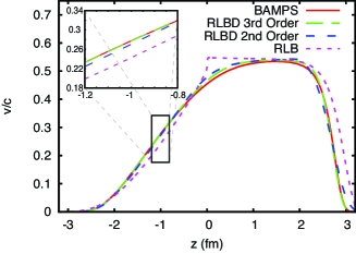
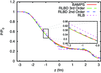
Figure 2: Velocity (top) and pressure (bottom) profiles as function of the $z$-coordinate for the case of a shockwave in quark-gluon plasma, with $\eta/s=0.1$.

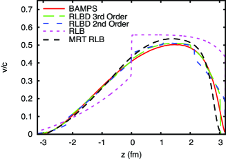
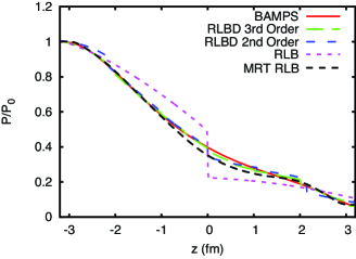
Figure 3: Velocity (top) and pressure (bottom) profiles as function of the $z$-coordinate for the case of a shockwave in quark-gluon plasma, with $\eta/s=0.5$.

In order to validate our model, we solve the Riemann problem for a quark-gluon plasma and compare the results with BAMPS and two previous relativistic Boltzmann models. The first one, proposed by Mendoza et al. Mendoza et al. (2010a, b) and later improved by Hupp et al. Hupp et al. (2011), which we will denote simply by RLB, and the second one, which is a recent extension of the RLB developed by Li et al. Li et al. (2012) to include multi-relaxation time, which we will denote by MRT RLB. BAMPS was developed by Xu and Greiner Xu and Greiner (2005) and applied to the Riemann problem in quark-gluon plasma by Bouras et al. Bouras et al. (2009). Since BAMPS solves the full relativistic Boltzmann equation, we take its result as a reference to access the accuracy of our model. However, we keep in mind that BAMPS also produces approximate solutions. The present model is hereafter denoted by RLBD (RLB with Dissipation).

For small ratios $\eta/s$, where $s$ is the entropy density, RLB and MRT RLB reproduced BAMPS results to a satisfactory degree of accuracy. However, for higher $\eta/s\geq 0.1$ and moderately fast fluids, $\gamma\sim 1.3$, RLB failed to reproduce the velocity and pressure profiles Hupp et al. (2011). MRT RLB yielded good agreement with the results at $\eta/s=0.1$, but presented notable discrepancies for $\eta/s=0.5$. The failure of both RLB and MRT RLB to solve the Riemann problem for high viscous fluids can be ascribed to their inability to recover the third order moment of the distribution Hupp et al. (2011); Li et al. (2012).

In this section, we will study the case of high $\eta/s\geq 0.1$ in a regime of moderate velocities. We perform the simulations on a lattice with $1\times 1\times 1600$ cells, only half of which are represented in our domain owing to symmetry condition (the other half is a mirror, in order to use periodic boundary conditions for simplicity). Therefore, our simulation consists of $1\times 1\times 800$ lattice sites, with $\delta x=0.008fm$ and $\delta t=\sqrt{41}\;0.008fm/c$ for RLBD third order, and $\delta t=0.024fm/c$ for RLBD second order.

The initial conditions for the pressure are $P_{0}=5.43\frac{GeV}{fm^{3}}$ and $P_{1}=0.339\frac{GeV}{fm^{3}}$. In numerical units, they correspond to $1.0$ and $0.062$, respectively. The initial temperature $z\geq 0$ is $T_{1}=200MeV$ (in numerical units $0.5$), and $T_{0}=400MeV$ for $z<0$, which corresponds to $1.0$ in numerical units. The entropy density $s$ is calculated according to the relation, $s=4n-n\ln(n/n^{\rm eq})$, where $n^{\rm eq}$ is the density calculated with the equilibrium distribution, $n^{\rm eq}=d_{G}T^{3}/\pi^{2}$, with $d_{G}=16$ being the degeneracy of the gluons.

The velocity and pressure profiles at $t=3.2\frac{fm}{c}$ with viscosity-entropy density ratios of $\eta/s=0.1$, are shown in Fig. 2. In this figure, we compare the results with BAMPS and RLB, where we can see that RLB presents a discontinuity at $z=0$, while both second order and third order RLBD get closer to the BAMPS solution. Since the only difference between second and third order RLBD is the third order moment of the distribution, we conclude that at relatively low $\eta/s$, the third order does not play a crucial role neither in the conservative dynamics nor dissipative dynamics of the system. However, note that at $z\sim 3fm$, the third order model provides an outstanding fit of the numerical results by BAMPS.

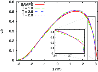
Figure 4: Velocity profile as function of the $z$-coordinate for the case of a shockwave in quark-gluon plasma, with $\eta/s=0.5$, by increasing the reference numerical temperature in the lattice, leading to a smaller relaxation time $\tau$.

On the other hand, by increasing the ratio $\eta/s$, we see from Fig. 3 that, while RLB gets worse and the second order RLBD fixes the discrepancy only in part, the 3rd order RLBD improves significantly the accuracy of the velocity and pressure profiles.

In Fig. 3, we also compare the results obtained with MRT RLB and BAMPS, for $\eta/s=0.5$. Here, we see that there is again an improvement, including the attainment of the right value of the maximum velocity (at $z\sim 1.5fm$). In the pressure profile, RLBD gets closer to BAMPS than MRT RLB in the region of the discontinuity in the initial condition ($z\sim 0$).

Note that there is a staircase shape in the results of RLBD for $\eta/s=0.5$ in Figs. 3. This is due to the large values taken by the single relaxation time in order to achieve such shear viscosity-entropy density ratios, $\tau\sim 20-40$ (in numerical units), which is beyond the hydrodynamic approximation and therefore higher order moments (fourth and higher orders) of the distribution function would be required, which is not fulfilled in our RLBD model. In order to prove this statement, we have performed separate simulations, see Fig. 4, where we observe that by increasing the value of the reference temperature of the lattice (typically set at $T=1$), so as to achieve the same shear viscosity, $\eta=(2/3)nT(\tau-1/2)/R$, the value of $\tau$ decreases and the staircase disappears. In particular, for $T\geq 2.5$, the results get closer to the ones with BAMPS, and become independent of the reference temperature. Unfortunately, due the discretization procedure used to develop this model, whenever the reference temperature $T>4$ the model becomes unstable, mostly likely because the expanded equilibrium distribution function takes negative values.

IV Conclusions and Discussions

We have introduced a new relativistic lattice Boltzmann model with improved dissipation, as compared to RLB and MRT RLB. To this purpose, we have performed an expansion of the Maxwell-Jüttner distribution onto an orthonormal basis of polynomials in the 4-momentum space. In addition, in order to make the model compatible with a regular cubic lattice, we have performed the expansion in cartesian coordinates and applied a time transformation, such that particles travel just the distance necessary to reach lattice nodes, always at the speed of light. The time transformation generates a sphere of radius $R$ which intersects the cubic lattice, the intersection points being lattice nodes by construction. In addition, we have reproduced up to second order moment of the equilibrium distribution, and up to third order moment, finding $R=3$ and $R=\sqrt{41}$ for second and third order moment compatibility, respectively.

The discrete energy component of the 4-momentum, $p^{0}$, has been calculated by using Gaussian quadrature, the nodes corresponding to the zeros of the next order polynomial. With this configuration, we need $90$ vectors for recovering second order and $384$ for the third order moment case. However, only $66$ and $128$, respectively, are actually needed to calculate the moments correctly.

In order to validate the model, we have compared our results with BAMPS, as well as previous RLB models. We have found that for $\eta/s=0.1$, our model accurately describes the Riemann problem in quark-gluon plasma, including the expansion up to second order. However, for the case of $\eta/s=0.5$, the second order model, although better than RLB, is less accurate than both MRT RLB and the third order model. The third order model yields better results than the previous RLB, but it develops a staircase shape as a consequence of the large value of the single relaxation time, which lies beyond the hydrodynamic regime. We have shown that the staircase pathology can be tamed by increasing the reference temperature in the model. Nevertheless, increasing the reference temperature beyond $T=4$ hits against stability limits of the model.

We may envisage that a multi-relaxation time extension of the present model would further improve the accuracy of the results. A similar improvement may be anticipated by implementing higher order expansions of the equilibrium distribution. However, since the transport coefficients depend on the collision operator, their calculation within a multi-relaxation time model becomes increasingly involved. On the other hand, by performing expansions to include higher order moments, the value of $R$ might become unpractically large, with several ensuing discretization issues. Notwithstanding such potential difficulties, these extensions are surely worth being analyzed in depth for the future.

Appendix A Second order relativistic lattice Boltzmann model

To construct the second order lattice Boltzmann model, we use the procedure described in this paper. We have obtained that $R=3$ presents enough symmetries to fulfill the conditions in Eqs. (22), and the velocity vectors $\vec{\vartheta}$ are given by, $(\pm 3,0,0)$, $(0,\pm 3,0)$, $(0,0,\pm 3)$, $(\pm 2,\pm 1,\pm 2)$, $(\pm 1,\pm 2,\pm 2)$, and $(\pm 2,\pm 2,\pm 1)$. The values for the discrete $p^{0}$ come from the solution of the equation,

$${\cal R}^{(3)}=\frac{1}{12}p^{0}(p^{0}-6)^{2}-2=0\quad,$$ (42)

instead of ${\cal R}^{(4)}$ for the case of the third order expansion. This gives the values $p_{l}^{0}\simeq 0.936$, $3.305$, and $7.759$. The discrete 4-momentum vectors $p_{i}^{\mu}$ are constructed with Eqs. (17), and (21), and they are in total, ${\cal N}=3\times 30=90$. However, as in the third order expansion, we have retained the minimal amount, out of $90$, that are necessary to recover the second order moment, by imposing the maximum number of $w_{i}$ to be zero. This gives only $66$ 4-momentum vectors. The value of the weight functions for every momentum vector and the relation with the $30$ directions are given in the Supplementary Material sup . In Fig. 5 we report the spatial configuration of the vectors $\vec{\vartheta}_{i}$.

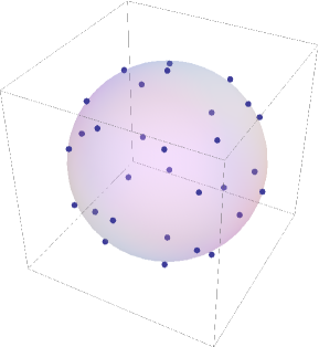
Figure 5: Directions of the velocity vectors $\vec{\vartheta}_{i}$ to recover up to the second order moment of the Maxwell-Jüttner distribution, namely the momentum-energy tensor. The radius of the sphere is $R=3$. The points represent lattice sites belonging to the surface of the sphere.

The discrete version of the relativistic Boltzmann equation, Eq. (38), still applies and the discrete equilibrium distribution function is written in detail in Appendix B, Eq. (43). However, due to the fact that the third order moment is not satisfied, an analytical theory to calculate the transport coefficients would be very complicated and goes beyond the scope of this work. Therefore, we have calculated numerically only the shear viscosity, by matching the results for low velocity with the third order moment model. This, in order to compare the results of both expansions with other models in the literature. This gives a shear viscosity $\eta_{\rm 2nd}\sim(1/7)P(\tau-\delta t/2)/R$. We could, in principle, calculate the third order moment associated with the equilibrium distribution given by Eq. (43), and, by applying the Grad method, compute the other transport coefficients. However, this procedure would need to be performed entirely numerically, since the weights $w_{i}$ and 4-momentum vectors $p_{i}^{\mu}$ are only known numerically. Since the main purpose of this paper is to improve the description of dissipative effects by performing the third order expansion and place it on a cubic lattice, we are not interested in the bulk viscosity and the thermal conductivity for this case, and leave this task for future work.

Appendix B Equilibrium Distribution Functions

The equilibrium distribution function capable to recover the first and second order moments of the equilibrium distribution is calculated by using up to the second order polynomials in Eq. (7), namely the $14$ polynomials $J_{k}$ with $k=0,...,13$, obtaining

$$f_{i}^{\rm eq} =\frac{nw_{i}}{4T}\bigg{[}{p_{i}^{0}}^{2}\left(T^{2}\left(2{U^{0}}^{2}-{U^{x}}^{2}-{U^{y}}^{2}-1\right)-2T{U^{0}}+1\right)+2{p_{i}^{0}}(T(T({U^{0}}({p_{i}^{x}}{U^{x}}+{p_{i}^{y}}{U^{y}}+{p_{i}^{z}}{U^{z}}-4{U^{0}})+1)$$ (43)

$$-{p_{i}^{x}}{U^{x}}-{p_{i}^{y}}{U^{y}}-{p_{i}^{z}}{U^{z}}+7{U^{0}})-4)+T^{2}\bigg{(}{p_{i}^{x}}^{2}\left(-{U^{0}}^{2}+2{U^{x}}^{2}+{U^{y}}^{2}+1\right)+2{p_{i}^{x}}{U^{x}}({p_{i}^{y}}{U^{y}}+{p_{i}^{z}}{U^{z}}-4{U^{0}})$$

$$+{p_{i}^{y}}^{2}\left(-{U^{0}}^{2}+{U^{x}}^{2}+2{U^{y}}^{2}+1\right)+2{p_{i}^{y}}{U^{y}}({p_{i}^{z}}{U^{z}}-4{U^{0}})+8{U^{0}}({U^{0}}-{p_{i}^{z}}{U^{z}})-2\bigg{)}$$

$$+2T(5({p_{i}^{x}}{U^{x}}+{p_{i}^{y}}{U^{y}}+{p_{i}^{z}}{U^{z}})-8{U^{0}})+12\bigg{]}\quad,$$

For the case of the third order moment expansion, we repeat the same procedure, using all the polynomials ($k=0,...,29$). This leads to the following expressions:

$$f_{i}^{\rm eq} =\frac{nw_{i}}{12T}\bigg{[}{p_{i}^{0}}^{3}(T{U^{0}}-1)\left(T^{2}\left(4{U^{0}}^{2}-3\left({U^{x}}^{2}+{U^{y}}^{2}+1\right)\right)-2T{U^{0}}+1\right)$$ (44)

$$-{p_{i}^{0}}^{2}\bigg{(}T^{3}\bigg{(}-2{U^{0}}^{2}(3{p_{i}^{x}}{U^{x}}+3{p_{i}^{y}}{U^{y}}+2{p_{i}^{z}}{U^{z}})+\left({U^{x}}^{2}+{U^{y}}^{2}+1\right)(3{p_{i}^{x}}{U^{x}}+3{p_{i}^{y}}{U^{y}}+{p_{i}^{z}}{U^{z}})$$

$$+36{U^{0}}^{3}-6{U^{0}}\left(3{U^{x}}^{2}+3{U^{y}}^{2}+4\right)\bigg{)}+3T^{2}\left(2{U^{0}}({p_{i}^{x}}{U^{x}}+{p_{i}^{y}}{U^{y}}+{p_{i}^{z}}{U^{z}})-22{U^{0}}^{2}+7\left({U^{x}}^{2}+{U^{y}}^{2}\right)+9\right)$$

$$-3T({p_{i}^{x}}{U^{x}}+{p_{i}^{y}}{U^{y}}+{p_{i}^{z}}{U^{z}}-14{U^{0}})-15\bigg{)}-3{p_{i}^{0}}\bigg{(}T^{3}\bigg{(}{U^{0}}^{3}\left({p_{i}^{x}}^{2}+{p_{i}^{y}}^{2}-24\right)-{U^{0}}\bigg{(}{p_{i}^{x}}^{2}\left(2{U^{x}}^{2}+{U^{y}}^{2}+1\right)$$

$$+2{p_{i}^{x}}{U^{x}}({p_{i}^{y}}{U^{y}}+{p_{i}^{z}}{U^{z}})+{p_{i}^{y}}\left({p_{i}^{y}}{U^{x}}^{2}+2{p_{i}^{y}}{U^{y}}^{2}+{p_{i}^{y}}+2{p_{i}^{z}}{U^{y}}{U^{z}}\right)-12\bigg{)}+12{U^{0}}^{2}({p_{i}^{x}}{U^{x}}+{p_{i}^{y}}{U^{y}}+{p_{i}^{z}}{U^{z}})$$

$$-2({p_{i}^{x}}{U^{x}}+{p_{i}^{y}}{U^{y}}+{p_{i}^{z}}{U^{z}})\bigg{)}+T^{2}\bigg{(}{p_{i}^{x}}^{2}\left(-{U^{0}}^{2}+2{U^{x}}^{2}+{U^{y}}^{2}+1\right)+2{p_{i}^{x}}{U^{x}}({p_{i}^{y}}{U^{y}}+{p_{i}^{z}}{U^{z}}-11{U^{0}})$$

$$+{p_{i}^{y}}^{2}\left(-{U^{0}}^{2}+{U^{x}}^{2}+2{U^{y}}^{2}+1\right)+2{p_{i}^{y}}{U^{y}}({p_{i}^{z}}{U^{z}}-11{U^{0}})-22{p_{i}^{z}}{U^{0}}{U^{z}}+56{U^{0}}^{2}-14\bigg{)}$$

$$+2T(6({p_{i}^{x}}{U^{x}}+{p_{i}^{y}}{U^{y}}+{p_{i}^{z}}{U^{z}})-25{U^{0}})+20\bigg{)}+T\bigg{(}{p_{i}^{x}}^{3}T^{2}{U^{x}}\left(-3{U^{0}}^{2}+4{U^{x}}^{2}+3{U^{y}}^{2}+3\right)$$

$$+{p_{i}^{x}}^{2}T\left(3\left({U^{0}}^{2}-2{U^{x}}^{2}-{U^{y}}^{2}-1\right)(-{p_{i}^{y}}T{U^{y}}+6T{U^{0}}-7)+{p_{i}^{z}}T{U^{z}}\left(-{U^{0}}^{2}+4{U^{x}}^{2}+{U^{y}}^{2}+1\right)\right)$$

$$+3{p_{i}^{x}}{U^{x}}\bigg{(}T\bigg{(}T\left({p_{i}^{y}}^{2}\left(-{U^{0}}^{2}+{U^{x}}^{2}+2{U^{y}}^{2}+1\right)+2{p_{i}^{y}}{U^{y}}({p_{i}^{z}}{U^{z}}-6{U^{0}})-12{p_{i}^{z}}{U^{0}}{U^{z}}+24{U^{0}}^{2}-4\right)$$

$$+14{p_{i}^{y}}{U^{y}}+14{p_{i}^{z}}{U^{z}}-48{U^{0}}\bigg{)}+30\bigg{)}+{p_{i}^{y}}^{3}T^{2}{U^{y}}\left(-3{U^{0}}^{2}+3{U^{x}}^{2}+4{U^{y}}^{2}+3\right)$$

$$+{p_{i}^{y}}^{2}T\left({p_{i}^{z}}T{U^{z}}\left(-{U^{0}}^{2}+{U^{x}}^{2}+4{U^{y}}^{2}+1\right)+3(6T{U^{0}}-7)\left({U^{0}}^{2}-{U^{x}}^{2}-2{U^{y}}^{2}-1\right)\right)$$

$$+6{p_{i}^{y}}{U^{y}}\left(T\left(2T\left(-3{p_{i}^{z}}{U^{0}}{U^{z}}+6{U^{0}}^{2}-1\right)+7{p_{i}^{z}}{U^{z}}-24{U^{0}}\right)+15\right)+6{p_{i}^{z}}{U^{z}}\left(2T^{2}\left(6{U^{0}}^{2}-1\right)-24T{U^{0}}+15\right)$$

$$-24{U^{0}}\left(T^{2}\left(2{U^{0}}^{2}-1\right)-5T{U^{0}}+5\right)\bigg{)}-30\left(T^{2}-2\right)\bigg{]}\quad.$$

References

- Novoselov et al. (2004) K. S. Novoselov, A. K. Geim, S. V. Morozov, D. Jiang, Y. Zhang, S. V. Dubonos, I. V. Grigorieva, and A. A. Firsov, Science 306, 666 (2004).
- Novoselov et al. (2005) K. Novoselov, A. Geim, S. Morozov, D. Jiang, M. Katsnelson, I. Grigorieva, and S. Dubonos, Nature Letters 438, 197 (2005).
- Müller et al. (2009) M. Müller, J. Schmalian, and L. Fritz, Phys. Rev. Lett. 103, 025301 (2009).
- Shuryak (2004) E. Shuryak, Progress in Particle and Nuclear Physics 53, 273 (2004), ISSN 0146-6410, heavy Ion Reaction from Nuclear to Quark Matter.
- Kovtun et al. (2005) P. K. Kovtun, D. T. Son, and A. O. Starinets, Phys. Rev. Lett. 94, 111601 (2005).
- Policastro et al. (2001) G. Policastro, D. T. Son, and A. O. Starinets, Phys. Rev. Lett. 87, 081601 (2001).
- Mendoza et al. (2010a) M. Mendoza, B. M. Boghosian, H. J. Herrmann, and S. Succi, Phys. Rev. Lett. 105, 014502 (2010a).
- Mendoza et al. (2010b) M. Mendoza, B. M. Boghosian, H. J. Herrmann, and S. Succi, Phys. Rev. D 82, 105008 (2010b).
- Benzi et al. (1992) R. Benzi, S. Succi, and Vergassola, Phys. Rep. 222, 145 (1992).
- Xu and Greiner (2005) Z. Xu and C. Greiner, Phys. Rev. C 71, 064901 (2005).
- Bouras et al. (2009) I. Bouras, E. Molnar, H. Niemi, Z. Xu, A. El, O. Fochler, C. Greiner, and D. H. Rischke, Phys. Rev. Lett. 103, 032301 (2009).
- Hupp et al. (2011) D. Hupp, M. Mendoza, I. Bouras, S. Succi, and H. J. Herrmann, Phys. Rev. D 84, 125015 (2011), URL http://link.aps.org/doi/10.1103/PhysRevD.84.125015.
- Romatschke et al. (2011) P. Romatschke, M. Mendoza, and S. Succi, Phys. Rev. C 84, 034903 (2011), URL http://link.aps.org/doi/10.1103/PhysRevC.84.034903.
- Cercignani and Kremer (2002) C. Cercignani and G. M. Kremer, The Relativistic Boltzmann Equation: Theory and Applications (Boston; Basel; Berlin: Birkhauser, 2002).
- He and Luo (1997) X. He and L.-S. Luo, Phys. Rev. E 56, 6811 (1997).
- Martys et al. (1998) N. S. Martys, X. Shan, and H. Chen, Phys. Rev. E 58, 6855 (1998), URL http://link.aps.org/doi/10.1103/PhysRevE.58.6855.
- Li et al. (2012) Q. Li, K. H. Luo, and X. J. Li, Phys. Rev. D 86, 085044 (2012), URL http://link.aps.org/doi/10.1103/PhysRevD.86.085044.
- Chikatamarla and Karlin (2006) S. S. Chikatamarla and I. V. Karlin, Phys. Rev. Lett. 97, 090601 (2006).
- Chikatamarla and Karlin (2009) S. S. Chikatamarla and I. V. Karlin, Phys. Rev. E 79, 046701 (2009).
- Anderson and Witting (1974) J. Anderson and H. Witting, Physica 74, 466 (1974).
- (21) See Supplementary Material at.