Radio light curves during the passage of cloud G2 near Sgr A^∗

Abstract

We calculate radio light curves produced by the bow shock that is likely to form in front of the G2 cloud when it penetrates the accretion disk of Sgr A^∗. The shock acceleration of the radio-emitting electrons is captured self-consistently by means of first-principles particle-in-cell simulations. We show that the radio luminosity is expected to reach maximum in early 2013, roughly a month after the bow shock crosses the orbit pericenter. We estimate the peak radio flux at $1.4\,\rm GHz$ to be $1.4-22\,\rm Jy$ depending on the assumed orbit orientation and parameters. We show that the most promising frequencies for radio observations are in the $0.1<\nu<1\,\rm GHz$ range, for which the bow shock emission will be much stronger than the intrinsic radio flux for all the models considered.

1 Introduction

The center of our Galaxy is known to host a black hole with a moderate mass of $M=4.3\times 10^{6}M_{\odot}$ (e.g., Genzel et al., 2010). This low-luminosity black hole, which is identified with the radio source Sgr A^∗, accretes at a very low accretion rate (see, e.g., Quataert et al. 1999), has not been observed to produce relativistic outflows, and only sporadically shows flares in X-rays (Baganoff et al. 2001). The quiet and unimpressive life of Sgr A^∗ is slated to change in the late summer of 2013 when a dense cloud of gas will approach it along a highly eccentric orbit (Gillessen et al., 2012a, b), with periapsis well inside the Bondi radius of the central black hole, $R_{\rm B}\approx 0.04\rm pc\approx 2\times 10^{5}R_{\rm G}$, where the gravitational radius is defined as $R_{\rm G}=GM/c^{2}=2\times 10^{-7}\rm pc$.

Gillessen et al. (2012a) discovered the gas cloud, called G2, during their extended observational campaign of stars in the vicinity of the Galactic Center. They estimated the cloud’s mass to be $\lesssim 3\;M_{\oplus}$ (Gillessen et al., 2012a) and determined the orbital parameters of its center of mass. A semi-major axis of $a=666\pm 39\rm mas$, eccentricity of $e=0.9664\pm 0.0026$, and epoch of periastron of $t_{0,\rm CM}=2013.69\pm 0.04$, yield a periapsis distance that is only $4400\pm 600R_{\rm G}$ from the black hole (Gillessen et al., 2012b). The interaction of the cloud with the accretion flow presents a unique opportunity to probe the local conditions of gas at radii $R\sim 10^{3.5}R_{\rm G}$. This corresponds to a few percent of the Bondi radius of Sgr A^∗ (Yuan et al., 2003) and is a largely unexplored region of the accretion flow around the black hole.

Using theoretical models of the accretion flow around Sgr A^∗, Narayan et al. (2012a) recently predicted that a bow shock will form ahead of G2 for a few months around the time of closest approach. This shock will likely accelerate particles and produce detectable levels of synchrotron radiation. The expected parameters of the shock correspond to a highly unusual regime for particle acceleration, one that has hardly been studied until now. Although the shock velocity is non-relativistic, at a temperature of $T\sim 10^{8.5}$ K the upstream electrons are nearly relativistic. Therefore, the electrons are more easily accelerated to high Lorentz factors and the injection problem often encountered in shock acceleration is mitigated. In addition, the unshocked gas will be already magnetized, leading to conditions that could be particularly ideal for seeing synchrotron radiation from particles accelerated by G2’s bow shock.

In this paper we extend the work by Narayan et al. (2012a) in several ways. We explore in more detail the propagation of G2 through the accretion flow around Sgr A^∗ using a general relativistic magnetohydrodynamic (GRMHD) numerical simulation of the pre-impact accretion flow (Narayan et al. 2012b). We consider various orientations of the orbit of G2 with respect to the accretion flow and utilize the simulation to determine the physical parameters of the pre-shock gas. We perform first-principles particle-in-cell calculations of particle acceleration in the shock for the range of physical parameters sampled along the orbit. We consider the net effect of particle acceleration along the cloud’s trajectory using two limiting approximations: one in which the moving cloud collects and holds on to all the relativistic electrons accelerated by the bow shock (the plowing case) and one in which electrons accelerated in the shock are left behind and radiate in the unshocked magnetic field (the local case). We calculate the spectrum of accelerated electrons along G2’s trajectory and the corresponding synchrotron radio light curves for these two possibilities.

The structure of the paper is as follows. In Section 2 we discuss the adopted model for the accretion flow around Sgr A^∗. In Section 3 we discuss the parametrization of the cloud orbit with respect to the disk equatorial plane. In Section 4 we show results of our study. We begin in Section 4.1 by calculating profiles of physical parameters of the accretion flow along the cloud orbit. In Section 4.2 we discuss the physics of electron acceleration and present the particle-in-cell simulations that we performed for relevant gas and shock parameters in order to provide estimates of the acceleration efficiency and the shape of the spectrum of non-thermal electrons. In Section 4.3 we present the predicted radio light curves and the spectrum of the radio emission from the bow shock and discuss their dependence on the orbit orientation. In Section 5, we comment on the uncertainties and optimal observing strategies of the G2 impact. Finally, we summarize our work in Section 6.

2 Model of Sgr A^∗ accretion disk

Accretion on to Sgr A^∗ is believed to occur via an advection-dominated accretion flow (ADAF: Narayan & Yi, 1994; Narayan & Yi, 1995; Narayan et al., 1995; Yuan et al., 2003; Narayan & McClintock, 2008). This mode of accretion is present whenever the mass accretion rate is low, roughly $<1\%$ of Eddington; hence, it operates in the vast majority of galactic nuclei in the Universe. In the case of Sgr A^∗, observations in radio, infrared and X-rays, coupled with theoretical models, have provided partial information on the parameters of the accretion flow. Yuan et al. (2003) used the number density of electrons at the Bondi radius $n_{\rm e}(R_{\rm B})\approx 130\,\rm cm^{-3}$ (Baganoff et al. 2003), along with a model of the radio and submillimeter emission from thermal electrons in the inner accretion disk, to estimate the mass accretion rate on to the black hole. They found $\dot{M}_{\rm BH}\approx 4\times 10^{-8}\,\rm M_{\odot}\,{\rm yr^{-1}}$. Other spectral models, based on radiative transfer calculations using post-processed numerical simulations of global accretion disks, led to somewhat lower estimates, $\dot{M}_{\rm BH}\approx 2\times 10^{-9}\,\rm M_{\odot}\,{\rm yr^{-1}}$ (Mościbrodzka et al., 2009), while measurements of Faraday rotation in the magnetized accreting gas gave values somewhere in between the two estimates: $\dot{M}_{\rm BH}\approx 10^{-8}\,\rm M_{\odot}\,{\rm yr^{-1}}$ (Marrone et al., 2007).

Although constraining, the results above do not specify the entire structure of the accretion flow. In particular, while the models are fairly reliable near the black hole and near the Bondi radius, they are poorly constrained at the intermediate radii probed by G2’s orbit. To fill in this gap, studies rely on numerical calculations. GRMHD simulations provide a proper treatment of the innermost regions as well as of the flow on larger scales.. Recently, a number of groups have studied radiatively inefficient accretion flows using such numerical models (e.g., De Villiers et al., 2003; Gammie et al., 2003; Anninos et al., 2005; Del Zanna et al., 2007; Narayan et al., 2012b; McKinney et al., 2012; , Tchekhovskoy & McKinney2012). For the work reported here, we make use of one of the ADAF models around a non-spinning black hole (spin parameter $a_{*}=0$) described in Narayan et al. (2012b). The simulated flow corresponds to a Magnetically Arrested Disk (MAD, Narayan et al. 2003), i.e., a system in which the poloidal magnetic field is strong enough to partially “arrest” the accreting gas. The MAD state is believed to be a reasonable approximation of most ADAFs in the Universe fed by gas with initially non-zero poloidal magnetic flux. The most important feature of the particular MAD simulation under consideration is that it was run for an unprecedentedly long time. The results reported in Narayan et al. (2012b) corresponded to a duration of $10^{5}GM/c^{3}$, but since then the simulation has been run further, up to a time of $2\times 10^{5}GM/c^{3}$. As a result, the accretion flow has achieved steady state out to a large radius $\sim 200R_{\rm G}$. This is important for the present work, as we explain below. The fact that the simulation assumes zero black hole spin, whereas the black hole in Sgr A^∗ probably has a moderate non-zero spin (Broderick et al., 2011), is not important since spin affects only the innermost regions of the accretion flow, whereas G2 interacts with gas that is much farther out.

At periapsis, G2 is estimated to be located at a radius of $R=4400R_{\rm G}$ from the black hole (Gillessen et al., 2012b). Therefore, in order to predict synchrotron emission from G2’s bow shock, we need to know the properties of the ambient accreting gas at this radius. However, no global GRMHD simulation can hope to obtain direct estimates at such large radii because of the prohibitive computational times required. Because of this, we extrapolate the physical quantities we obtained from smaller radii. Such an extrapolation is acceptable, provided that the simulation has reached steady state out to a large enough radius where the flow shows self-similar behavior (at small radii, the influence of the black hole causes large deviations from self-similarity.) This is what makes the MAD simulation described above particularly good for the present application. Having reached steady state out to radii $R\sim 200R_{\rm G}$, the flow properties in this simulation have almost certainly entered the self-similar regime (see Narayan et al. 2012b). Hence, we may safely extrapolate out to the radii of interest to us. In the present work, we choose $R=150R_{\rm G}$ as the anchor radius from which we carry out the extrapolation.

We present in Figure 1 the radial profiles of density (top-left), temperature (top-right), azimuthal velocity (bottom-left) and magnetic to gas pressure ratio (bottom-right). We plot the MAD simulation results for $R\leq 150R_{\rm G}$ (left of the vertical solid line) and show power-law extrapolations at larger radii, $R\geq 150R_{\rm G}$. We indicate the radius corresponding to G2’s periapsis with the vertical dash-dotted line. The various colors and line thicknesses correspond to different values of the polar angle $\theta$.

We adjusted the density normalization to match the measured density at the Bondi radius, $n_{\rm e}(R_{\rm B})=130\,\rm cm^{-3}$ (Baganoff et al. 2003), using a power-law extrapolation $R^{-1}$. The corresponding mass accretion rate at the black hole is $\dot{M}_{\rm BH}=5\times 10^{-8}\rm M_{\odot}/yr$, which is consistent with the estimates given above. The slope we chose for the density extrapolation differs from the canonical slope for an ADAF disk $R^{-3/2}$. However, as emphasized by Yuan et al. (2012a, b), an $R^{-1}$ profile provides a better description of nearly all global ADAF simulations to date This is true of our MAD simulation as well. Especially in the vicinity of the equatorial plane, we see that the simulation results at smaller radii match seamlessly to an $R^{-1}$ extrapolated power-law at larger radii. As expected, the largest densities are found at the equatorial plane ($\theta=\pi/2$) and the smallest near the polar axis ($\theta=0$).

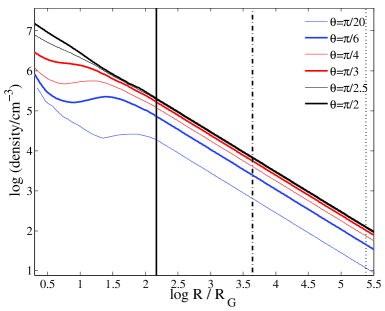
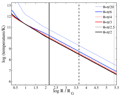
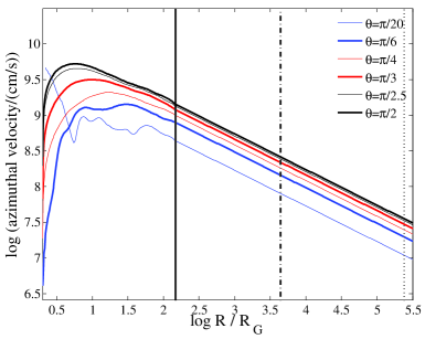
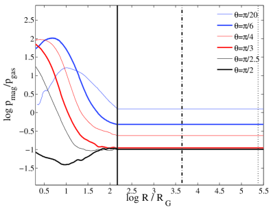
Figure 1: Numerical disk model and its extrapolation. Panels show logarithms of density (top left), gas temperature (top right), azimuthal velocity (bottom left), and magnetic to gas pressure ratio (bottom right panel). Vertical lines show the radius of extrapolation ($R=150R_{\rm G}$, solid), the periapsis of the cloud orbit ($R=4400R_{\rm G}$, dot-dashed) and the Bondi radius ($R=2\times 10^{5}R_{\rm G}$, dotted). $\theta$ is the polar angle and $\theta=\pi/2$ corresponds to the equatorial plane.

The profiles of gas temperature show equally good convergence. These again show an $R^{-1}$ dependence, indicating that the gas temperature scales proportional to the virial temperature. At a given radius, the hottest gas is above the disk surface, near the polar axis. The simulation does not distinguish between the ion and electron temperatures, whereas detailed ADAF models generally allow for a two temperature gas with $T_{i}\neq T_{e}$ (Narayan & Yi 1995). In most models, the plasma becomes two-temperature only at radii well below $10^{3}R_{G}$ (e.g., Fig. 2 in Narayan et al. 1995). At larger radii, Coulomb collisions between protons and electrons are sufficiently frequent to enforce a single temperature. For the model of the accretion flow employed in the present work, the Coulomb equilibration time between protons and electrons at pericenter of G2 is $\sim 10^{6}\,\rm s$, which is shorter than the orbital time by a factor of $\sim 50$ (and of course, shorter than the radial accretion time by an even larger factor).

The azimuthal velocity scales with radius according to the expected Keplerian dependence $R^{-1/2}$. At a given radius, the largest azimuthal velocity is seen at the equatorial plane. The further from the disk plane, the slower is the rotation. We assume the radial and vertical (in $\theta$) velocities to be zero.

The magnetic to gas pressure ratio shows the worst convergence among the four quantities shown. Only inside the bulk of the disk does it settle down to a relatively radius-independent value $\sim 0.1$, which is a typical value for most MHD accretion disks (but see Gaburov et al. 2012 for a discussion of the impact of the initial magnetic field configuration on the saturated value of the pressure ratio). Off the mid-plane, the gas is strongly magnetized and the pressure ratio does not settle down to a constant value even at $R=150R_{\rm G}$. Thus, extrapolation under the assumption of a constant ratio is not well justified. However, this will have relatively little impact on the light curves when compared to other uncertainties (see Section 5).

For convenience, in Appendix A we give analytic formulae which reasonably approximate the disk structure for $R>150R_{\rm G}$.

3 Orbit orientation

The orbital parameters of the center of mass of G2 are well constrained (Gillessen et al., 2012b). In this work we assume that the shock follows precisely this orbit, neglecting possible hydrodynamical interactions between the cloud and disk gas which might affect the cloud front. Modeling these hydrodynamic effects will require MHD simulations that include both the moving cloud and the orbiting accretion flow, which we will present in future work.

The cloud orbital plane is inclined with respect to the observer’s line-of-sight and is roughly aligned with the well-known ring of stars around Sgr A^∗ (Bartko et al. 2009; Levin & Beloborodov 2003). The orientation of the accretion disk around Sgr A^∗ is, however, poorly constrained. Therefore, in this paper, we allow the full range of possible relative orientations between the cloud orbital plane and the disk plane. Given the uncertainties in our model (see Section 5), it is unlikely, but not impossible, that the observed lightcurve will put constraints on the disk orientation.

Because of the assumed axisymmetry of the accretion flow, the following two angles completely specify the geometry: the inclination angle, $i$, and the argument of periapsis, $\omega$. Figure 2 shows a three-dimensional visualisation of three sample orbits whose orbital parameters correspond to those of G2. The inclination $i$ corresponds to the angle between the orbital plane of G2 and the equatorial plane of the accretion disk. Cloud orbits that counter-rotate with respect to the disk correspond to $i<\pi/2$, while co-rotating orbits correspond to $\pi/2<i<\pi$. The argument of periapsis $\omega$ is the angle between the line connecting the black hole and orbit pericenter and the line of nodes where the two planes cross. The orbits shown in the figure correspond to $\omega=0$ (green), $\pi/4$ (blue) and $\pi/2$ (purple line).

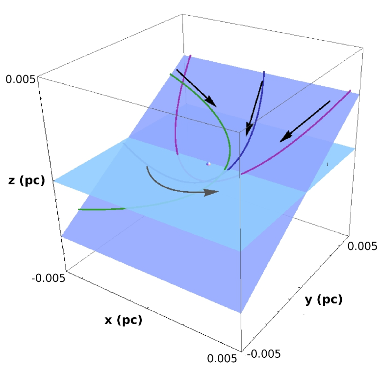
Figure 2: Three-dimensional visualisation of the orbit orientation. The orbital plane is inclined to the disk plane by an angle $i$. The argument of periapsis for the orbits shown is $\omega=0$, $\pi/4$ and $\pi/2$ for green, blue and purple orbits, respectively. The arrows denote the cloud direction of motion and the disk rotation.

The cloud crosses the disk equatorial plane twice during each full orbit. The locations and times of these crossings depend on $\omega$, but not $i$. Figure 3 shows as a function of $\omega$ the epochs when the two crossings occur for the cloud center of mass (CM). For $\omega=0$ (green orbit in Fig. 2), one of the crossings takes place exactly at periastron ($t=2013.69$), while the other occurs half an orbital period, i.e., $\sim 100\,\rm yr$ later. For $\omega=\pi/4$, the CM crossings take place at $t=2013.57$ and $t=2015.49$. For $\omega=\pi/2$, the disk equatorial plane crossings are symmetric with respect to periastron and occur at $t=2013.33$ and $2014.06$.

time (yr)
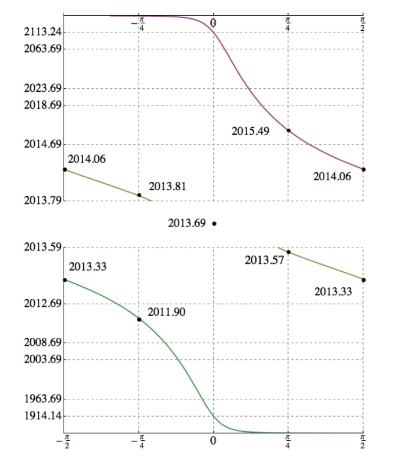
	$\omega\,\,\rm(rad)$

Figure 3: Crossing time of the disk equatorial plane (in years) by the cloud center of mass as a function of the argument of periapsis $\omega$. The vertical axis is non-uniform and follows the logarithm of $t-t_{0,\rm CM}$, where $t_{0,\rm CM}$ is the epoch of pericenter for the center of mass. Points and labels denote crossing times for $\omega=-\pi/2$, $-\pi/4$, $0$, $\pi/4$, and $\pi/2$.

The particular choices of $i$ and $\omega$ that we considered in this work are listed in Table 1 where the crossing times are given relative to the epoch of pericenter $t_{0}$.

Table 1: Orbit orientation parameters

Inclination ($i$)
$\pi/3$	counter-rotating
$\pi/4$	counter-rotating
$\pi/6$	counter-rotating
$\pi-\pi/3$	co-rotating
$\pi-\pi/4$	co-rotating
$\pi-\pi/6$	co-rotating

Argument	Disk equatorial plane crossings
of periapsis ($\omega$)	relative to the epoch of pericenter $t_{0}$
$0$	single crossing at $t=t_{0}$
$\pi/4$	two asymmetric crossings at $t=t_{0}-0.12\rm yr$ and $t_{0}+1.8\rm yr$
$\pi/2$	symmetric crossings at $t=t_{0}-0.37\rm yr$ and $t_{0}+0.37\rm yr$

4 Results

4.1 Accretion gas properties along the orbit

The radio synchrotron emission that we expect as a function of time as G2 orbits around Sgr A^∗ depends on the properties of the ambient accretion disk at various points along the orbit. Key quantities are the density, temperature and magnetic field strength in the ambient gas, and the Mach number of the cloud relative to the gas. Using the extrapolated profiles discussed in Section 2, it is straightforward to compute all these quantities along the orbit as a function of time for a given choice of the cloud orbital parameters, $i$ and $\omega$.

The top-most panels in Figure 4 show the variation of density along the orbit. The columns correspond to inclination angles $i=\pi/3$ (left, high inclination; but also $i=\pi-\pi/3$, since the scalar fields are identical when reflected), $\pi/4$ (middle), and $\pi/6$ (right, low inclination). In Figure 4, colors denote orbits with different values of the argument of periapsis $\omega$. The horizontal axis shows time relative to the epoch of periastron $t_{0}$. The green lines correspond to $\omega=0$, where the cloud crosses the disk equatorial plane only once, at pericenter. Consequently, all these density curves have a single maximum at $t=t_{0}$. Blue curves correspond to $\omega=\pi/4$, where the cloud crosses the disk plane twice. For the high inclination case there are two local maxima. The first one corresponds roughly to the first crossing of the equatorial plane ($t=t_{0}-0.12$), while the second occurs much earlier than the second crossing ($\sim t_{0}+0.3$ vs $t_{0}+1.8$) because of the fact that the decrease of density with increasing radius dominates over the effect of the latitude away from the midplane. The second peak is not visible for low inclinations because in these cases the cloud never goes very far from the mid-plane in between the two crossings. For the same reason, all the density curves in the last column (low inclination case) lie almost on top of each other. Indeed, in the limit $i\to 0$ (which corresponds to the orbital plane coinciding with the disk plane), $\omega$ will have no impact on any of the curves.

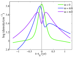
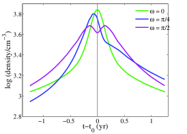
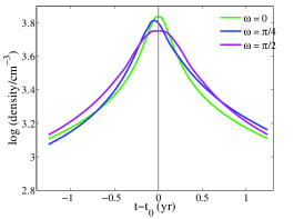
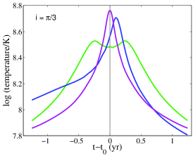
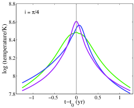
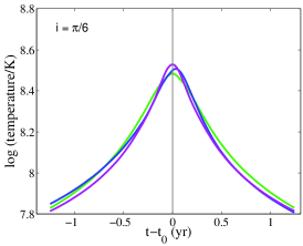
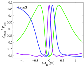
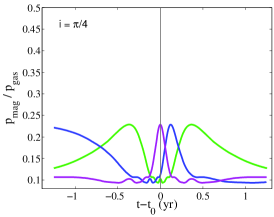
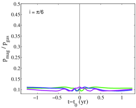
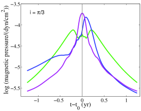
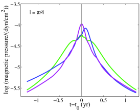
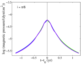
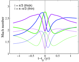
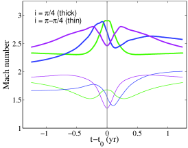
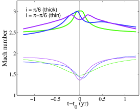
Figure 4: Profiles of (from top to bottom) density, temperature, magnetic to gas pressure ratio, magnetic pressure and Mach number along the cloud orbit for inclinations: $i=\pi/3$ (left), $\pi/4$ (middle) and $\pi/6$ (right column) as a function of time ($t_{0}$ denotes the epoch of pericenter of the shock front). Thick and thin lines in the bottom-most set of panels correspond to counter- and co-rotating orbits, respectively. Colors denote the value of the argument of periapsis $\omega$ and correspond to the orbits shown in Fig. 2.

The second row of panels shows the variation of temperature along the cloud orbit. As discussed in Section 2, at a given radius the temperature is the lowest at the mid-plane and increases towards the polar axis. As a result, for the highly inclined orbit shown in the left panel, the green curve in which the orbit crosses the disk plane exactly at pericenter has twin peaks, a few months before and after pericenter. This is when the cloud comes closest to the polar axis and encounters the hottest gas. The opposite behavior is seen for the purple curve with two symmetric disk plane crossings. Here, there is a single peak in the temperature exactly at pericenter, when the cloud moves away from the mid-plane. As in the case of the density, for orbits with low inclinations, all the curves are similar.

The third row of panels shows the magnetic to gas pressure ratio. Close to the mid-plane this parameter is approximately equal to $0.1$, while closer to the poles it takes on larger values. Qualitatively, the behavior is similar to that of the temperature, except that, being a ratio of pressures, there is no variation with radius. The shapes of the various curves in the different panels are then easy to understand. The fourth row of panels shows the magnetic pressure $P_{\rm mag}=B^{2}/8\pi$. This quantity does vary with radius and behaves quite a lot like the temperature. Thus, the curves show striking similarity to those shown in the second row of panels.

Finally, the bottom row of panels shows the cloud Mach number with respect to the disk gas. Here two sets of curves are plotted for each choice of $i$ and $\omega$, thick curves for counter-rotating orbits (inclination $=i$) and thin curves for co-rotating orbits (inclination $=\pi-i$). As expected, the Mach number is lower for co-rotating orbits. Also, the difference between counter- and co-rotating orbits increases for lower inclinations (the two curves coincide for an orbit perpendicular to the disk plane, $i=\pi/2$). The Mach number for counter-rotating orbits lies in the range $1.8-3.0$ while for co-rotating orbits it is in the range $1.3-2.0$. Most importantly, we find that the Mach number is always greater than unity in all cases. This means that a bow shock is expected to form for every orientation of the orbit and thus we always expect some level of excess synchrotron emission from shock-accelerated electrons.

4.2 Electron acceleration in the bow shock of G2

A variety of astrophysical evidence suggests that particles are accelerated efficiently via the Fermi and shock-drift acceleration mechanisms in shocks (e.g., Blandford & Eichler 1987). Typically, these processes give rise to a non-thermal power-law tail in the energy distribution of the particles. The parameters of the bow shock of G2 correspond to an interesting regime that has not been well studied. The shock is non-relativistic, but the upstream electrons are quasi-relativistic (assuming thermal equilibrium between electrons and protons), with temperature varying between $T\simeq 10^{8.0}K$ and $T\simeq 10^{8.7}K$ along the cloud orbit (see the second row of panels in Fig. 4). As a result of the relatively hot temperature in the accretion flow, the shock has a modest Mach number, ranging between ${\cal M}\approx 1.5$ and ${\cal M}\approx 3$ (see the bottom-most row of panels in Fig. 4).

We studied the acceleration of electrons in the bow shock of G2 by means of two-dimensional first-principles numerical simulations, with the particle-in-cell code TRISTAN-MP (Spitkovsky 2005). The simulation setup parallels closely the one employed by Riquelme & Spitkovsky (2011) and Narayan et al. (2012a), with the magnetic field lying initially in the simulation plane, oriented at an oblique angle with respect to the flow velocity. We fixed the angle between the upstream field and the shock velocity to be $\psi=63^{\circ}$, and the ratio of magnetic to gas pressure in the accretion flow to be $P_{\rm mag}/P_{\rm gas}=0.1$. Below, we argue that the same acceleration physics operates across a wide range of magnetic obliquities, and for ratios of magnetic to gas pressure as large as $P_{\rm mag}/P_{\rm gas}=0.5$ (see the third row of panels in Fig. 4). We explored the dependence of our results on the pre-shock temperature over the range $10^{8.1}K$ up to $10^{8.7}$ K, as appropriate for the region closest to the cloud pericenter where most of the emission will be produced, and on the shock Mach number, which we varied between $2$ and $3.5$.

For computational convenience, we chose a reduced mass ratio $m_{\rm p}/m_{\rm e}=100$, but we verified that our results remain the same for larger mass ratios, when all the physical quantities are scaled appropriately. Specifically, we ran simulations spanning the range $m_{\rm p}/m_{\rm e}=25-400$, fixing the pre-shock electron temperature (equal to the proton temperature), the shock Mach number and the ratio of magnetic to gas pressure, and we measured the time in units of the inverse proton cyclotron frequency $\omega_{\rm ci}^{-1}$. We also checked the convergence of our results with respect to the spatial resolution and the number of computational particles per cell (up to 128 per cell).

We find that at the shock, a fraction of the incoming electrons are reflected backward by the shock-compressed magnetic field (Matsukiyo et al. 2011) or by scattering off of electron whistler waves excited in the shock transition layer (Riquelme & Spitkovsky 2011). For quasi-relativistic electron temperatures, the reflected electrons are fast enough to remain ahead of the shock, resisting advection downstream by the oblique pre-shock field. As the shock-reflected electrons gyrate around the shock, they get energized by shock-drift acceleration (e.g., Begelman & Kirk 1990) and form a local non-thermal population, just upstream of the shock. The constraint that the reflected electrons be fast enough to outrun the shock along the oblique field, thus participating in the shock-drift acceleration, can be recast as an upper limit on the field obliquity $\psi$. If the characteristic electron thermal velocity is $v_{\rm th,e}=\sqrt{kT/m_{\rm e}}$ and the shock velocity is $v_{\rm sh}$, electron acceleration is possible only if $\psi\lesssim\psi_{\rm crit}$, where the critical obliquity angle $\psi_{\rm crit}$ satisfies $v_{\rm th,e}\cos\psi_{\rm crit}=v_{\rm sh}$. So, the criterion for efficient electron acceleration can be rewritten as

$$\psi\lesssim\psi_{\rm crit}\simeq\arccos\left({\cal M}\sqrt{m_{\rm e}/m_{\rm p}}\right)~{},$$ (1)

showing that, even for our largest Mach number (${\cal M}=3.5$), electron acceleration will be a common by-product of the shock evolution, being allowed for all angles $\psi\lesssim 85^{\circ}$, if we take the realistic mass ratio $m_{\rm p}/m_{\rm e}=1836$. For our reduced mass ratio $m_{\rm p}/m_{\rm e}=100$, we chose the obliquity angle $\psi=63^{\circ}$ so that the constraint $\psi\lesssim\psi_{\rm crit}$ required for efficient electron acceleration is satisfied for all the shock Mach numbers that we investigated.

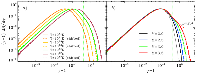
Figure 5: Electron energy spectrum just upstream of the shock, normalized to the pre-shock electron density, for parameters relevant to the orbit of G2. (Left) Electron energy spectrum at $\omega_{\rm ci}t=10.8$ for different upstream temperatures, but fixed Mach number ${\cal M}=3$. The spectra plotted with dashed lines have been shifted along the $x$-axis by $(T/10^{8.5}K)^{-1}$, to normalize the energy scale. (Right) Electron energy spectrum at $\omega_{\rm ci}t=10.8$ for different Mach numbers, but fixed electron temperature $T=10^{8.5}K$. In both panels, the vertical green dotted line marks the location of the low-energy end of the electron power-law tail, whose slope $p\simeq 2.4$ is indicated as a red dashed line in the right panel. In the right panel, the black dotted curve shows a Maxwellian distribution with $T=10^{8.5}K$.

As demonstrated by Narayan et al. (2012a) for a pre-shock flow with temperature $T=10^{9}K$, the electrons participating in the shock-drift acceleration process are accelerated ahead of the shock into a power-law tail with a slope $p\simeq 2.2$ and containing roughly $5\%$ of the incoming electrons (i.e., the so-called acceleration efficiency is $\eta\simeq 0.05$). The upper energy cutoff of the pre-shock electron spectrum steadily increases and the slope becomes flatter over time, suggesting that the distribution will asymptote at late times to a power-law tail with $p\lesssim 2.2$ extending to very large electron energies (we refer to the left panel of Fig. 2 in Narayan et al. (2012a) for details on the temporal evolution of the electron spectrum). The electron energization at early times is governed by the shock-drift mechanism, but the diffusive Fermi process is expected to dominate at late times. We find that the counter-streaming between the incoming flow and the shock-reflected electrons triggers the Weibel filamentation instability ahead of the shock (Weibel 1959, Medvedev & Loeb 1999), with the wavevector perpendicular to the pre-shock field. By scattering off of the turbulence generated by the Weibel instability, the electrons pre-accelerated by the shock-drift mechanism will be injected into the Fermi process.

If the electron acceleration in our simulations is still primarily controlled by the shock-drift mechanism, the electron energy gain $\Delta\gamma\,m_{\rm e}c^{2}$ during a time $\Delta t$ will be

$$\Delta\gamma\,m_{\rm e}c^{2}\sim q\,E\,v_{\rm e/\!/}\,\Delta t~{},$$ (2)

where $E$ is the strength of the background motional electric field (originating from the drift of the upstream frozen-in magnetic field toward the shock) and $v_{\rm e/\!/}$ is the component of the electron velocity along the electric field. By taking $v_{\rm e/\!/}\sim v_{\rm th,e}$ (or a few times larger than $v_{\rm th,e}$), we can rewrite the expression above as

$$\frac{\Delta\gamma\,m_{\rm e}c^{2}}{kT}\sim{\cal M}\sin\psi\sqrt{\frac{m_{\rm p}}{m_{\rm e}}}\;\omega_{\rm ci}\,\Delta t~{},$$ (3)

which can be used to interpret the dependence of our results on the pre-shock conditions, as we now describe.

In Figure 5, we show how the electron spectrum ahead of the shock depends on the upstream temperature (left panel, with fixed Mach number ${\cal M}=3$) and on the shock Mach number (right panel, with fixed temperature $T=10^{8.5}K$). In the left panel, we present the electron spectrum ahead of the shock for four values of the flow temperature: $T=10^{8.1}K$ (orange solid curve), $T=10^{8.3}K$ (yellow solid curve), $T=10^{8.5}K$ (green solid curve) and $T=10^{8.7}K$ (purple solid curve). The location of the thermal peak in the electron spectrum scales linearly with the pre-shock temperature. When we rescale our spectra to account for this effect (i.e., we shift them along the $x$-axis by $(T/10^{8.5}K)^{-1}$), the resulting distributions nearly overlap (compare the green solid line with the three dashed curves). The electron power-law tail starts at $\gamma-1\simeq\xi\,kT/m_{\rm e}c^{2}$, where $\xi\simeq 7.5$ is nearly insensitive to the pre-shock temperature (vertical green dotted line), and the tail contains about $5\%$ of the incoming electrons. The fact that electron spectra for different upstream temperatures are identical, modulo an overall shift in the energy scale, can be easily understood from Eqs. (1) and (3). The former demonstrates that the condition for efficient injection into the acceleration process does not depend explicitly on the flow temperature, at fixed Mach number. In addition, Eq. (3) shows that the temporal evolution of the high-energy spectral cutoff, normalized to the thermal peak, is insensitive to the upstream temperature.

The dependence of the electron spectrum on the shock Mach number is illustrated in the right panel of Figure 5, showing that the non-thermal tail is most pronounced in high-${\cal M}$ shocks. Yet, some evidence for electron acceleration to non-thermal energies is present even in the spectrum of ${\cal M}=2$ shocks (black solid line), whose high-energy end clearly departs from a Maxwellian distribution (black dotted line). We point out that the main difference among shocks with different Mach number is not in the normalization of the non-thermal tail or in the location of its low-energy end, but in the extent of the power-law component. Regardless of the Mach number, the tail contains a fraction $\sim 5\%$ of the incoming electrons, and its low-energy end is at $\gamma-1\simeq\xi\,kT/m_{\rm e}c^{2}$, where $\xi\simeq 7.5$ is nearly insensitive to the shock Mach number (vertical green dotted line). The fact that the acceleration efficiency is independent of the Mach number follows from Eq. (1), since $\psi\lesssim\psi_{\rm crit}$ for all of our choices of ${\cal M}$. Also, the increase in the high-energy spectral cutoff with Mach number is in agreement with Eq. (3), stating that the acceleration rate scales linearly with ${\cal M}$. It follows that, at a given time (in units of $\omega_{\rm ci}^{-1}$), the spectrum of shocks with higher Mach number will have stretched to more extreme energies.

The non-thermal tail in the electron spectrum of ${\cal M}=3.5$ shocks (red solid line) can be fitted as a power law of slope $p\simeq 2.4$ (red dashed line). We expect the power-law tail to become flatter with time, as its high-energy cutoff increases, and the spectral slope $p$ should approach the value $p\simeq 2.2$ found by Narayan et al. (2012a) in a flow with $T=10^{9}K$. In shocks with ${\cal M}\lesssim 3$ (black, blue and green curves), given the limited extent of the power-law tail, it is still premature to draw firm conclusions regarding the appropriate value of the power-law slope at late times. Below, we assume that, regardless of ${\cal M}$, the power-law tail in steady state will have a slope $p=2.4$. As discussed above, this is likely to be a conservative upper limit, since the power-law index at late times is expected to approach the value $p\simeq 2.2$ obtained by Narayan et al. (2012a).

We have also tested that neither the acceleration efficiency nor the spectral slope depend significantly on the ratio of magnetic to gas pressure (we have tried $P_{\rm mag}/P_{\rm gas}=0.1$, 0.3 and 0.5) or the obliquity angle $\psi$, provided that $\psi\lesssim\psi_{\rm crit}$. In fact, from Eqs. (1) and (3), we expect that the ratio $P_{\rm mag}/P_{\rm gas}$ should not appreciably change the spectral shape, whereas the field obliquity (in the range $\psi\lesssim\psi_{\rm crit}$) should only affect the evolution of the high-energy spectral cutoff, as illustrated in Eq. (3).

4.3 Radio lightcurves

As we showed in the previous sections, the bow shock that will form ahead of the cloud G2 as it moves supersonically through the ambient disk gas is likely to accelerate, via the mechanism described in the previous subsection, the already hot electrons to relativistic energies. The original thermal distribution of electrons will thus be modified and a high energy power law tail will develop. When these high energy electrons gyrate magnetic field present in the disk, they emit synchrotron radiation. As we will show below, under favorable circumstances, the emission from the shocked electrons can overwhelm the steady-state radio emission from Sgr A^∗.

In our calculations we assume the following parameters to calculate the total number of accelerated electrons. We take the cloud cross section (the transverse area of the shock perpendicular to the relative velocity between the cloud and the accretion flow) to be $A=\pi R^{2}$, with $R=10^{15}{\rm cm}$, and use an electron acceleration efficiency equal to $\eta=0.05$. We take the low-energy end of the power-law tail at $\gamma-1=\xi(kT/m_{\rm e}c^{2})$, where $\xi=7.5$ and $T$ is the electron temperature, and the slope of the high-energy tail as $p=2.4$.

Whether or not the shocked electrons will remain close to the shock is unclear. We, therefore, consider two distinct limiting cases. In one scenario, which we call the plowing model, we assume that all relativistic electrons remain in the shocked gas and radiate in the instantaneous shock-compressed magnetic field. In the second scenario, referred to as the local model, we assume that the shocked electrons are left behind at their original position in the accretion flow while the cloud and the shock move on, and that the electrons radiate in the original uncompressed field. We believe that the real situation will be somewhere between these two extremes.

4.3.1 Results from the plowing model

In the plowing model, all the accelerated electrons remain in the vicinity of the shock. Because of the long synchrotron cooling timescale ($>100\,\rm yrs$, see Narayan et al. 2012a), there is no loss of accelerated particles and hence the number of radiating relativistic electrons at each energy increases monotonically with time. However, this does not imply a monotonically increasing luminosity since the synchrotron emissivity varies with the magnetic field strength. The field in the shocked gas is proportional to the field in the ambient accretion flow, which varies as a function of position along the orbit. As discussed in the previous section (see Fig. 4), after an initial increase, the magnetic field strength drops as the cloud moves away from the central black hole. Therefore, while we expect an initial rapid increase in the synchrotron luminosity (since both the number of relativistic electrons and the magnetic field strength increase as the cloud approaches periapsis), this will be followed by a slower decay (the number of shocked electrons will continue to increase but the magnetic field will drop with time).

To calculate the lightcurve, we pre-compute the positions and velocities of the cloud as a function of time for given orbit angles $i$ and $\omega$. For each differential time interval between $t$ and $t+\Delta t$, we calculate the energy distribution of electrons accelerated in that interval,

$$\frac{{\rm d}N}{{\rm d}\gamma}_{\rm local}=Av\Delta tn_{e}\eta\frac{(p-1)(\xi kT/m_{\rm e}c^{2})^{p-1}}{(\gamma-1)^{p}}\quad\text{for}\,\gamma-1>\xi(kT/m_{\rm e}c^{2}),$$ (4)

where $n_{e}$ is the local disk number density and $v$ is the velocity of the cloud relative to the gas. The differential distributions are summed to obtain the total distribution of electrons at any given time according to

$$\frac{{\rm d}N}{{\rm d}\gamma}(t,\gamma)=\sum_{n=1}^{N(t)}\frac{{\rm d}N}{{\rm d}\gamma}_{\rm local},$$ (5)

where the sum goes over all the time steps up to the given time $t$.

The spectral synchrotron power is calculated using the standard formula for a power-law distribution of electrons (Rybicki & Lightman, 1979),

$$P_{\nu}(t)=\frac{\sqrt{3}q^{3}CB}{m_{\rm e}c^{2}(p+1)}\Gamma\left(\frac{p}{4}+\frac{19}{12}\right)\Gamma\left(\frac{p}{4}-\frac{1}{12}\right)\left(\frac{2\pi m_{\rm e}c\nu}{3qB}\right)^{-\frac{p-1}{2}},$$ (6)

where

$$C=\frac{{\rm d}N}{{\rm d}\gamma}(t,\gamma=2).$$ (7)

The strength of the magnetic field $B$ is given by

$$B=\frac{(\hat{\gamma}+1){\cal M}^{2}}{(\hat{\gamma}-1){\cal M}^{2}+2}B_{\rm disk},$$ (8)

which accounts for the amplification of the ambient disk magnetic field $B_{\rm disk}$ by a compression factor that depends on the shock Mach number ${\cal M}$ and the adiabatic index $\hat{\gamma}=5/3$. Note that only the component of the field perpendicular to the shock normal is amplified and that, for the sake of simplicity, we ignore the longitudinal component here. Taking into account the distance to Sgr A^∗ as $D=8.3\rm kpc$, we obtain the observed synchrotron flux as

$$F_{\nu}(t)=\frac{P_{\nu}(t)}{4\pi D^{2}}.$$ (9)

Figure 6 shows a set of lightcurves calculated with the above procedure for $\nu=1.4\,\rm GHz$ (where self-absorption is negligible, see Section 4.4). The rows correspond to different inclination angles, starting from $i=\pi/3$ (top), through $i=\pi/4$ (middle), to $i=\pi/6$ (bottom), while the columns correspond, from left to right, to different arguments of periapsis, $\omega=0$, $\pi/4$, and $\pi/2$. The thick and thin lines refer to counter- and co-rotating orbits, respectively. All the curves show the expected behavior, i.e., a relatively sharp increase when the cloud approaches pericenter, followed by a slower decay when the cloud and the shocked electrons move to regions with a weaker magnetic field. For all orbit inclinations, the radio emission is predicted to start rising a few months before the shock reaches pericenter. Co-rotating orbits produce significantly weaker emission due to the lower relative velocity of the cloud with respect to the gas, which results in a smaller number of accelerated electrons as well as a weaker shock-compressed field (since the shock Mach number is smaller). The maximal flux for counter-rotating orbits is in the range $13-22\,\rm Jy$, with the exact value depending on the orbit orientation. For co-rotating orbits, the range is $3-7\,\rm Jy$. In most cases, the maximal emission is occurs roughly a month after the shock reaches periapsis. For some orbit orientations two peaks are predicted in the light curve.

	$\omega=0$	$\omega=\pi/4$	$\omega=\pi/2$
$i=\pi/3$
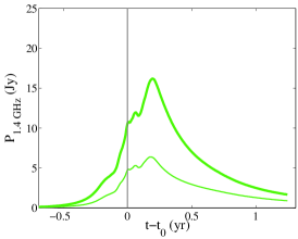
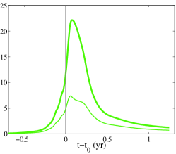
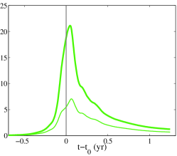
$i=\pi/4$
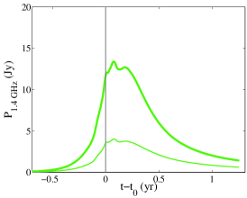
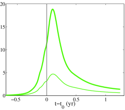
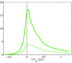
$i=\pi/6$

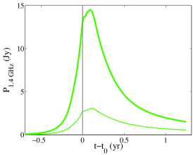
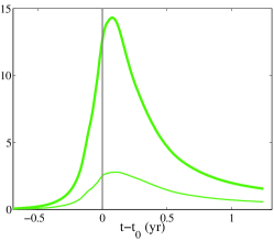
Figure 6: Radio lightcurves at 1.4 GHz for different orbit orientations assuming the plowing model for acceleration (Section 4.3.1). Rows correspond to inclination angles $i=\pi/3$, $\pi/4$ and $\pi/6$ (top to bottom). Columns correspond to the argument of periapsis $\omega=0$, $\pi/4$ and $\pi/2$ (left to right). Thick and thin lines are for counter- and co-rotating orbits, respectively. The vertical line corresponds to the bow shock epoch of periastron $t_{0}$.

4.3.2 Results from the local model

In the local model, electrons are assumed to move out of the shocked region and to remain in their original location in the accretion flow, radiating in the original uncompressed magnetic field. We neglect adiabatic expansion losses of the accelerated electrons, since the expansion time is typically larger than the evolution timescale of the cloud along its orbit. In this approximation, each accelerated electron radiates under the same conditions throughout the entire period of the cloud encounter; hence, the procedure described in the previous section has to be modified. Equation 4, which describes the energy distribution of electrons accelerated in a given time step, still holds, but instead of summing up the number of electrons and calculating the emission, here we sum up the radiation from electrons at each location that are accelerated in all the time steps up to a given time $t$, i.e.,

$$P_{\nu}(t)=\sum_{n=1}^{N(t)}P_{\nu,\,\rm local}(t),$$ (10)

where $P_{\nu,\,\rm local}(t)$ is calculated via Equation (6) but with

$$C=\frac{{\rm d}N}{{\rm d}\gamma}_{\rm local}(t,\gamma=2).$$ (11)

This last quantity corresponds to the number of accelerated electrons in a given time step at time $t$ and $B=B_{\rm disk}$ is the original uncompressed disk magnetic field.

By construction, in the local model, the emission increases monotonically with time. However, because the magnetic field is not amplified, the total emission is lower than in the plowing model. Figure 7 shows a set of light curves that exhibit exactly such behavior. All of the curves start to increase a few months before the shock reaches pericenter but none of them reaches a flux that significantly exceeds $4\,\rm Jy$. The difference in the magnitude of the maximum flux between the plowing and local models, which is roughly a factor of 5, is caused by two factors. First, the magnetic field is weaker in the local model than in the plowing model, leading to a corresponding decrease in the synchrotron emissivity. Second, because the accelerated electrons are not accumulated in the local model, fewer electrons reach the most favorable radius for emission. Depending on the orbit orientation, the maximal flux at $1.4\,\rm GHz$ lies in the $1.4-4.1\,\rm Jy$ range.

	$\omega=0$	$\omega=\pi/4$	$\omega=\pi/2$
$i=\pi/3$
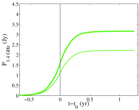
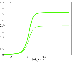
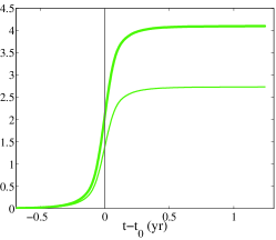
$i=\pi/4$
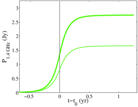
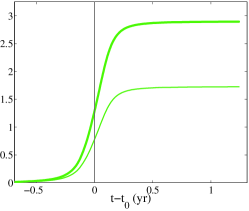
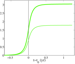
$i=\pi/6$

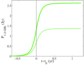
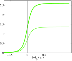
Figure 7: Similar to Figure 6 but for the local model (Section 4.3.2).

4.4 Spectra

In the preceding calculations, we assumed that the energy distribution of the shocked electrons is described by a single power law with slope $p=2.4$. This results in a power-law synchrotron spectrum ($F_{\nu}\propto\nu^{\alpha}$) with spectral index $\alpha=-(p-1)/2$ (Eq. 6), which implies that the flux is highest at low frequencies. However, at very low frequencies, the emission is limited by synchrotron self-absorption, which was estimated by Narayan et al. (2012a) to affect frequencies $\nu\lesssim 1\rm GHz$. In this section, we calculate synchrotron self-absorption for the parameters adopted in this work and plot the expected spectral energy distribution.

Synchrotron emission at a given frequency is self-absorbed when its total intensity, calculated according to Equation (6), exceeds the intensity of the local blackbody emission at the characteristic temperature corresponding to the energy of electrons responsible for emission at that frequency. The emission is then limited to the blackbody value.

Synchrotron emission peaks at frequency $\nu$ for electrons with Lorentz factor $\gamma$ given by (Rybicki & Lightman, 1979),

$$\gamma^{2}\approx\frac{4\pi m_{\rm e}c\nu}{3qB},$$ (12)

which corresponds to a temperature $T$ equal to

$$T\approx\frac{\gamma m_{\rm e}c^{2}}{3k_{\rm B}}.$$ (13)

The spectral power emitted by a black body with this temperature from a surface area $A$ is

$$P_{\nu,\,{\rm BB}}=A\pi B_{\nu}(T),$$ (14)

where $B_{\nu}(T)$ is the intensity of blackbody radiation,

$$B_{\nu}(T)=\frac{2h\nu^{3}}{c^{2}}\frac{1}{e^{h\nu/kT}-1}.$$ (15)

The critical frequency below which self-absorption limits the synchrotron emission is given by the condition

$$P_{\nu,\,\rm BB}=P_{\nu},$$ (16)

where $P_{\nu}$ is given by Equation (6) or Equation (10). For simplicity, we will not treat the transition regime in detail. Instead, we will assume that the total spectrum can be represented as a broken power law, with a slope equal to $-(p-1)/2$ in the high-frequency range and equal to $5/2$ in the low-frequency segment that is self-absorbed below the critical frequency.

In the case of the plowing model, we assume that the radiating electrons are contained within a sphere of radius $R=10^{15}\rm cm$ and $A=4\pi R^{2}$. For the local model, we correct the emission for self-absorption independently at each cloud location assuming that the differential emitting area is $\Delta A=2\pi R\rm\Delta r$, where $\rm\Delta r$ corresponds to the distance covered by the cloud between time $t$ and $t+\Delta t$. Thus, the emitting area is effectively the surface of a tube of radius $R$ traced by the cloud moving along its orbit.

Figure 8 shows our calculated spectra at $t=t_{0}+0.05$ for the most and least favorable orbit orientations considered in this work. The left and right panels correspond to the top-right and bottom-left panels in Figures 6 and 7, respectively, i.e., to orbit orientations producing the most and the least amount of emission. The solid lines in Figure 8 correspond to the plowing model and the dashed lines to the local model. As before, thick and thin lines represent the counter- and co-rotating orbits, respectively. The flux levels obtained with the various models extend over a wide range, reflecting our lack of knowledge of the orbit orientation as well as the bow shock structure.

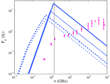
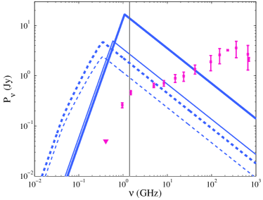
Figure 8: Spectra of bow shock synchrotron emission for most ($i=\pi/3$, $\omega=\pi/2$, left) and least ($i=\pi/6$, $\omega=\pi/2$, right panel) favorable orbit orientation (out of the orientations considered) calculated at $t=t_{0}+0.05$. Solid and dashed lines correspond to the plowing and local acceleration models, respectively. Thick lines show counter-rotating orbits while thin lines denote co-rotating orbits. Magenta points show the quiescent radio emission from Sgr A^∗ . The vertical line shows the frequency $\nu=1.4\,\rm GHz$ for which the lightcurves have been calculated.

The magenta data points in Figure 8 show the intrinsic radio emission of Sgr A^∗ compiled from the literature (Davies et al., 1976; Falcke & Markoff, 2000; Zhao et al., 2003; Marrone et al., 2008). If bow shock-related synchrotron radiation is to be unequivocally detected, the emission must exceed the quiescent emission of Sgr A^∗. It is clear that, at frequencies above $100\,\rm GHz$, none of the models predicts a detectable level of emission. The maximum emission in the plowing model occurs at $\sim 1\rm GHz$ and the flux here is well above the intrinsic emission of Sgr A^∗ . However, at the same frequency, the local model predicts the bow shock emission to be roughly comparable to the intrinsic flux. All our models predict detectable emission at levels above the intrinsic emission of Sgr A^∗ at frequencies in the range $0.1<\nu<1\,\rm GHz$.

4.5 When is $t_{0}$?

All of the light curves and spectra we calculated so far are expressed as a function of relative time with respect to the time $t_{0}$ when the bow shock reaches pericenter. The exact time corresponding to $t_{0}$ is unfortunately uncertain. Since the bow shock is expected to form in front of the cloud, $t_{0}$ is certainly earlier than the time $t_{0,\rm CM}$ when the cloud CM reaches pericenter. However, the exact location of the bow shock is poorly constrained. As a rough estimate, we can assume that the shock forms at the location corresponding to the “surface” of the original spherical cloud at $t=2000.0$, i.e., at a distance $R=1.5\times 10^{15}\rm cm$ (Gillessen et al., 2012a) ahead of the cloud CM along the orbit. This particular location precedes CM by $\sim 5$ months. Therefore, we estimate the time at which the bow shock reaches pericenter to be $t_{0}\approx 2013.2$, i.e., the bow shock should reach pericenter in March 2013. Naturally, this estimate is rather approximate since the internal structure of the cloud is unknown.

5 Discussion

5.1 Uncertainties

Apart from the uncertainty in $t_{0}$ discussed above, the model adopted here for calculating radio light curves relies on a number of other simplifications and assumptions. The most crucial of these is the adopted cross section of the shock region, which determines the number of shocked electrons and, therefore, the intensity of emission. We assumed that the effective area is constant in time, $A=\pi R^{2}$, with $R=10^{15}\,\rm cm$ corresponding to $2/3$ of the half-width at half-maximum as measured by Gillessen et al. (2012a). However, given that the cloud density is much larger than the density of the surrounding gas, it is possible that it will effectively plow gas with even larger area, thus increasing the magnitude of the flux enhancement.

A related uncertainty arises from the assumed shape of the cloud. G2 is not expected to keep its spherical shape throughout the passage: simulations show that the tidal gravitational field will first elongate it along the orbit, then squeeze it in the orbital plane at pericenter (Gillessen et al., 2012a; Saitoh et al., 2012), and finally let it decompress. However, the spatial extent of the cloud is large and the whole cloud will not become compressed at the same time. In other words, when the center of mass reaches the pericenter, only the middle part of the cloud is squeezed while its front has already decompressed and the tail lags behind.

To quantify the effects of tidal compression, we calculated the trajectories of $5000$ test particles following the approach of Gillessen et al. (2012a). We adopted the set of parameters given therein: a spherical cloud at $t=2000.0$ with Gaussian distribution of density with full-width at half-maximum (FWHM) equal $3\times 10^{15}\,\rm cm$ and a velocity dispersion $\sigma_{v}=130\,\rm km/s$. At four epochs ($t=2000.0$, $2013.0$, $2013.69$ and $2014.5$), we projected each particle onto the plane perpendicular to its nearest section of the cloud orbit and plotted their distribution in Figure 9. Due to the large density of the cloud when compared to the disk, the whole region covered by test particles may be considered likely to plow the gas. The black circle corresponding to $R=10^{15}\,\rm cm$ is always well within the projected cloud cross section. Our value is, therefore, rather conservative and the actual radio fluxes may be significantly stronger than those given in Section 4.3 if the effective area is indeed larger. In such a case, the critical frequency for the self-absorption will decrease, leading to higher flux at low frequencies, which may make the bow-shock emission easier to observe in that frequency range.

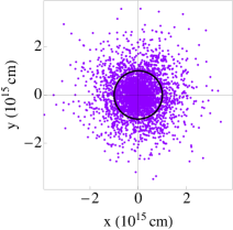
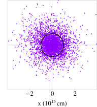
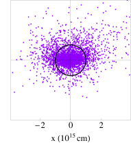
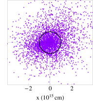
Figure 9: Cloud profile on a plane perpendicular to its orbit calculated with $5000$ test particles for (left to right) $t=2000.0$, $2013.0$, $2013.69$ (epoch of periastron) and $2014.5$. The black circle shows the region within $R=10^{15}\,\rm cm$ corresponding to the assumed cloud crossection.

In Section 4.2 we discussed the mechanism of electron acceleration. Given the long computational time required to obtain the power-law index of the accelerated electrons, we used only a coarse sampling of physical parameters throughout each potential orbit of the cloud. However, the impact of this coarse gridding is not overwhelming. For example, taking a power-law index $p=2.6$ instead of $p=2.4$ drives the calculated fluxes down only by a factor of $\sim 2$ and does not alter our conclusions regarding detectability. On the other hand, the value $p=2.4$ adopted here is likely to be a conservative upper limit. As described in section 4.2, the electron non-thermal tail should evolve toward flatter slopes at later times, approaching the value $p=2.2$ adopted by Narayan et al (2012a).

Finally, we note that there are uncertainties arising from the model for the accretion disk. While the gas temperature should always be close to virial, the disk density is poorly constrained by direct observations between the known values at the Bondi radius and the innermost regions where there is an estimate of the accretion rate (see also Psaltis 2012). We adopted a density profile $\rho\propto R^{-1}$ in between these two limits. In principle, the density may be a more complicated function of radius, which could lead to a different density along the orbit than predicted here. Given that the radio fluxes computed here are directly proportional to the local density of the accretion flow, they can easily be scaled for other models of the accretion flow.

5.2 Suggested Radio Monitoring Observations

The calculations presented in this paper indicate that the observed radio emission from Sgr A^∗  should undergo a significant brightening around or shortly after the pericentric passage of the bow shock, i.e., in spring 2013, assuming $t_{0}$ corresponds to March 2013 (see Section 4.5). In fact, given the $\sim 22$ mas displacement of the expected bow shock from the center of the accretion flow, where the long-term radio emission originates, the bow shock emission should appear as a new radio source that is, in principle, resolvable from the existing emission (Narayan et al. 2012a). In addition, we showed here that, under both the plowing and the local acceleration model assumptions, the spectrum of the bow shock emission should be different from that of quiescent emission in a number of ways. First, the emission is expected to peak at lower frequencies, around $\sim 0.3-1$ GHz. Second, the bow shock should produce detectable emission at $\nu\lesssim 1$ GHz, where the quiescent radio emission is undetectable.

The Karl V. Jansky Very Large Array (JVLA) is ideally positioned to detect and monitor the radio flux from the bow shock of G2 at frequencies around 1 GHz and above. Our “local” case with the least favorable orbit orientation produces the lowest level of flux enhancement. It nevertheless predicts a flux of 1.4 Jy at 1.4 GHz, which is comparable to the current quiescent flux from Sgr A^∗  at that frequency (see Figure 8). The plowing case, on the other hand, produces a radio signal that can be an order of magnitude or more higher than the current flux at 1.4 GHz but is shorter lived, with the flux enhancement decaying on a timescale of the order of a year. Monitoring the Galactic Center with the JVLA in 2013, therefore, should be able to not only detect the new radio emission from the bow shock but also to clearly distinguish the plowing and local models we considered here.

Given that the spectrum of the bow shock emission may also peak below 1 GHz for certain orbit orientations and acceleration models, as we discussed in Section 4, monitoring the Galactic Center at frequencies ranging from $\lesssim 100$ MHz to 1 GHz provides another optimal opportunity to probe the shock physics and the conditions of the accretion flow around pericenter. Furthermore, because Sgr A^∗  does not normally produce emission at these low frequencies, the detection of a bright radio source will deliver a definitive signature of the emission associated with G2. To this end, the Giant Metrewave Radio Telescope (GMRT), which operates at 5 frequencies between 50 MHz and 610 MHz, as well as at 1.4 GHz, is ideally placed and provides a strong complement to the JVLA. Given its latitude of 19^∘N, it is at a highly favorable location to observe the Galactic Center. In addition, GMRT has a distinct advantage in collecting area owing to 30 dishes with 45 m diameter each.

We encourage frequent monitoring at available bands between 50 MHz and 100 GHz during 2013 in order to capture the increase in the flux from Sgr A^∗ , to measure its rise time, and to detect the possible decay a year after pericentre.

6 Summary

The G2 cloud is expected to penetrate the accretion flow near Sgr A^∗ with a supersonic velocity and shock the gas in front of it. We showed that the shock parameters and the pre-shock electron temperatures are conducive to accelerating electrons to relativistic energies. These electrons can emit synchrotron radiation in the magnetic field of the accreting gas.

In this paper, we presented detailed predictions for radio light curves during the passage of the cloud. We adopted a state-of-the-art global numerical solution of a radiatively inefficient accretion flow as a base for our disk model and obtained physical disk parameters at large distances by extrapolating the numerical solution from within its converged, steady-state region. The parameters describing the electron acceleration process were determined by a set of particle-in-cell numerical simulations set up for the expected conditions as a function of the flow temperature and the shock Mach number. We considered a set of possible orientations of the orbit with respect to the accretion disk and two models for the particle acceleration: the plowing case, where all the electrons are kept in the shocked region and radiate in the shock-amplified magnetic field, and the local model, where the accelerated electrons are left behind the cloud front and radiate in their local, unshocked magnetic fields.

In both models, assuming the bow shock leads the cloud CM by half a year, we found that the radio luminosity is expected to reach peak values in spring 2013. For the plowing scenario this maximum will be followed by a decay, while for the local scenario the luminosity will stay constant due to the long cooling time of electrons. Calculated maximum luminosities at $\nu=1.4\,\rm GHz$ span the range $1.4-22\,\rm Jy$, depending on the adopted orbit orientation and acceleration mode, and are likely to exceed the intrinsic luminosity of Sgr A^∗ . At lower frequencies, the predicted emission will overwhelm the intrinsic luminosity for all the models considered by roughly an order of magnitude. We, therefore, recommend an observational campaign in 2013 at frequencies in the range $100\,{\rm MHz}-1\,{\rm GHz}$.

7 Acknowledgements

We thank Dimitrios Psaltis for useful comments. A.S. and R.N. were supported in part by NASA grant NNX11AE16G. L.S. is supported by NASA through Einstein Postdoctoral Fellowship grant number PF1-120090 awarded by the Chandra X-ray Center, which is operated by the Smithsonian Astrophysical Observatory for NASA under contract NAS8-03060. F.Ö. acknowledges support from NSF grant AST-1108753 and from the Radcliffe Institute for Advanced Study at Harvard University. The particle-in-cell simulations were performed on the Odyssey cluster at Harvard University, on XSEDE resources under contract No. TG-AST120010, and on NASA High-End Computing (HEC) resources through the NASA Advanced Supercomputing (NAS) Division at Ames Research Center.

Appendix A Approximated model for Sgr A^∗ accretion flow

For convenience, we give here analytical fits to the vertical structure of the disk at radius $R=150R_{\rm G}$, based on the GRMHD simulation discussed in Section 2. These profiles may be used to anchor extrapolations of disk properties to larger radii $R>150R_{\rm G}$. Table 2 gives expressions for vertical profiles of density, temperature, azimuthal velocity and magnetic to gas pressure ratio together with the proposed slopes for radial extrapolation. Radial and vertical velocities may be neglected. Figure 10 compares the numerical solution (red solid) with the fits (black dashed lines). The fits were obtained by least squares fitting to functions corresponding to expressions in Table 2 in the region $0.15<\theta<\pi-0.15$. The region closest to the polar axis is least reliable and was not taken into account.

Table 2: Analytical fits to disk vertical structure at $R=150R_{\rm G}$

quantity	fit	extrapolation
density [$\rm cm^{-3}$]	$\rho(\theta)=2.02\times 10^{5}\left(1-\left(\frac{\theta-\pi/2}{\pi/2}\right)^{2}\right)^{1.69}$	$\propto R^{-1}$
temperature [$\rm K$]	$\log T(\theta)=9.95+0.24\left(|\theta-\pi/2|\right)^{2.93}$	$\propto R^{-1}$
$\phi$ velocity [$\rm cm/s$]	$\log v_{\phi}(\theta)=9.15-0.24\left(|\theta-\pi/2|\right)^{2.04}$	$\propto R^{-1/2}$
$\chi=P_{\rm mag}/P_{\rm gas}$	$\chi(\theta)=0.1+0.31\left(|\theta-\pi/2|\right)^{3.89}$	$\propto R^{0}$

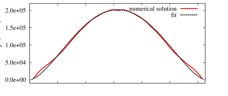
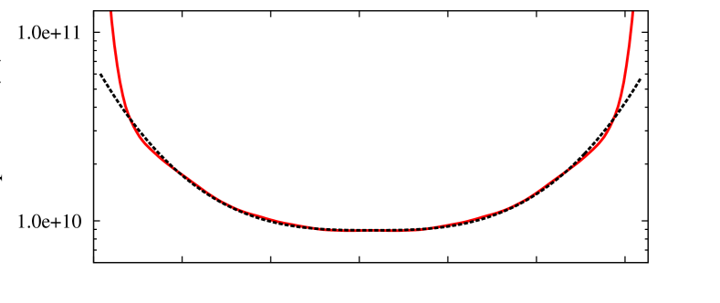
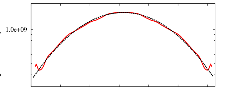
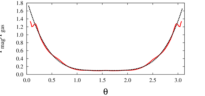
Figure 10: Vertical profiles of (top to bottom) density, gas temperature, azimuthal velocity, and magnetic to gas pressure ratio at $R=150R_{\rm G}$ for the numerical solution (red solid) and the analytical fit given in Table 2 (black dashed line). $\theta$ is the polar angle and $\theta=\pi/2$ corresponds to the equatorial plane.

References

- Anninos et al. (2005) Anninos, P., Fragile, P. C., & Salmonson, J. D. 2005, Astrophysical Journal, 635, 723
- Baganoff et al. (2001) Baganoff, F. K., Bautz, M. W., Brandt, W. N., et al. 2001, Nature, 413, 45
- Baganoff et al. (2003) Baganoff, F. K., Maeda, Y., Morris, M., et al. 2003, Astrophysical Journal, 591, 891
- Bartko et al. (2009) Bartko, H., Martins, F., Fritz, T. K., et al. 2009, Astrophysical Journal, 697, 1741
- Begelman & Kirk (1990) Begelman, M. C. & Kirk, J. G. 1990, Astrophysical Journal, 353, 66
- Blandford & Eichler (1987) Blandford, R. & Eichler, D. 1987, Physical Reports, 154, 1
- Broderick et al. (2011) Broderick, A. E., Fish, V. L., Doeleman, S. S., & Loeb, A. 2011, Astrophysical Journal, 735, 110
- Chan et al. (2009) Chan, C.-k., Liu, S., Fryer, C. L., et al. 2009, Astrophysical Journal, 701, 521
- Davies et al. (1976) Davies, R. D., Walsh, D., & Booth, R. S. 1976, Monthly Notices of the Royal Astronomical Society, 177, 319
- Del Zanna et al. (2007) Del Zanna, L., Zanotti, O., Bucciantini, N., & Londrillo, P. 2007, Astronomy & Astrophysics, 473, 11
- De Villiers et al. (2003) De Villiers, J.-P., Hawley, J. F., & Krolik, J. H. 2003, Astrophysical Journal, 599, 1238
- Falcke & Markoff (2000) Falcke, H., & Markoff, S. 2000, Astronomy & Astrophysics, 362, 113
- Gaburov et al. (2012) Gaburov, E., Johansen, A., & Levin, Y. 2012, Astrophysical Journal, 758, 103
- Gammie et al. (2003) Gammie, C. F., McKinney, J. C., & Tóth, G. 2003, Astrophysical Journal, 589, 444
- Genzel et al. (2010) Genzel, R., Eisenhauer, F., & Gillessen, S. 2010, Reviews of Modern Physics, 82, 3121
- Gillessen et al. (2012a) Gillessen, S., Genzel, R., Fritz, T. K., et al. 2012a, Nature, 481, 51
- Gillessen et al. (2012b) Gillessen, S., Genzel, R., Fritz, T. K., et al. 2012b, arXiv:1209.2272
- Levin & Beloborodov (2003) Levin, Y., & Beloborodov, A. M. 2003, Astrophysical Journal Letters, 590, L33
- Marrone et al. (2008) Marrone, D. P., Baganoff, F. K., Morris, M. R., et al. 2008, Astrophysical Journal, 682, 373
- Marrone et al. (2007) Marrone, D. P., Moran, J. M., Zhao, J.-H., & Rao, R. 2007, Astrophysical Journal Letters, 654, L57
- Matsukiyo et al. (2011) Matsukiyo, S., Ohira, Y., Yamazaki, R., & Umeda, T. 2011, ApJ, 742, 47
- Matsumoto et al. (2012) Matsumoto, Y., Amano, T., & Hoshino, M. 2012, ApJ, 755, 109
- McKinney et al. (2012) McKinney, J. C., Tchekhovskoy, A., & Blandford, R. D. 2012, Monthly Notices of the Royal Astronomical Society, 423, 3083
- Mościbrodzka et al. (2009) Mościbrodzka, M., Gammie, C. F., Dolence, J. C., Shiokawa, H., & Leung, P. K. 2009, Astrophysical Journal, 706, 497
- Narayan et al. (2003) Narayan, R., Igumenshchev, I. V., & Abramowicz, M. A. 2003, Publications of the Astronomical Society of Japan, 55, L69
- Narayan & McClintock (2008) Narayan, R., & McClintock, J. E. 2008, NAR, 51, 733
- Narayan et al. (2012a) Narayan, R., Özel, F., & Sironi, L. 2012a, Astrophysical Journal Letters, 757, L20
- Narayan et al. (2012b) Narayan, R., Sadowski, A., Penna, R. F., & Kulkarni, A. K. 2012b, MNRAS, accepted
- Narayan & Yi (1994) Narayan, R., & Yi, I. 1994, Astrophysical Journal Letters, 428, L13
- Narayan & Yi (1995) Narayan, R., & Yi, I. 1995, Astrophysical Journal, 452, 710
- Narayan et al. (1995) Narayan, R., Yi, I., & Mahadevan, R. 1995, Nature, 374, 623
- (32) Tchekhovskoy A., McKinney J. C., 2012, Monthly Notices of the Royal Astronomical Society, 423, L55
- Quataert et al. (1999) Quataert, E., Narayan, R., & Reid, M. J. 1999, Astrophysical Journal Letters, 517, L101
- Pang et al. (2011) Pang, B., Pen, U.-L., Matzner, C. D., Green, S. R., & Liebendörfer, M. 2011, Monthly Notices of the Royal Astronomical Society, 415, 1228
- Pen et al. (2003) Pen, U.-L., Matzner, C. D., & Wong, S. 2003, Astrophysical Journal Letters, 596, L207
- Psaltis (2012) Psaltis, D. 2012, Astrophysical Journal, 759, 130
- Riquelme & Spitkovsky (2011) Riquelme, M. A., & Spitkovsky, A. 2011, ApJ, 733, 63
- Rybicki & Lightman (1979) Rybicki, G. B., & Lightman, A. P. 1979, New York, Wiley-Interscience, 1979. 393 p.,
- Saitoh et al. (2012) Saitoh, T. R., Makino, J., Asaki, Y., et al. 2012, arXiv:1212.0349
- Spitkovsky (2005) Spitkovsky, A. 2005, in AIP Conf. Ser., Vol. 801, 345
- Vallado (2007) Vallado, D. A. 2007, Fundamentals of Astrodynamics and Applications, by D.A. Vallado. Berlin: Springer, 2007. ISBN: 978-0-387-71831-6,
- Weibel (1959) Weibel, E. S. 1959, Physical Review Letters, 2, 83
- Yuan et al. (2012b) Yuan, F., Bu, D., & Wu, M. 2012, Astrophysical Journal, 761, 130
- Yuan et al. (2003) Yuan, F., Quataert, E., & Narayan, R. 2003, Astrophysical Journal, 598, 301
- Yuan et al. (2012a) Yuan, F., Wu, M., & Bu, D. 2012, Astrophysical Journal, 761, 129
- Zhao et al. (2003) Zhao, J.-H., Young, K. H., Herrnstein, R. M., et al. 2003, Astrophysical Journal Letters, 586, L29