url]http://www-dft.ts.infn.it/ rfantoni/

Hellmann and Feynman theorem versus diffusion Monte Carlo experiment

Abstract

In a computer experiment the choice of suitable estimators to measure a physical quantity plays an important role. We propose a new direct route to determine estimators for observables which do not commute with the Hamiltonian. Our new route makes use of the Hellmann and Feynman theorem and in a diffusion Monte Carlo simulation it introduces a new bias to the measure due to the choice of the auxiliary function. This bias is independent from the usual one due to the choice of the trial wave function. We used our route to measure the radial distribution function of a spin one half Fermion fluid.

An important component of a computer experiment of a many particles system, a fluid, is the determination of suitable estimators to measure, through a statistical average, a given physical quantity, an observable. Whereas the average from different estimators must give the same result, the variance, the square of the statistical error, can be different for different estimators. We will denote with $\langle{\cal O}\rangle_{f}$ the measure of the physical observable ${\cal O}$ and with $\langle\ldots\rangle_{f}$ the statistical average over the probability distribution $f$. In this communication we use the word estimator to indicate the function ${\cal O}$ itself, unlike the more common use of the word to indicate the usual Monte Carlo estimator $\sum_{i=1}^{\cal N}{\cal O}_{i}/{\cal N}$ of the average, where $\{{\cal O}_{i}\}$ is the set obtained evaluating ${\cal O}$ over a finite number ${\cal N}$ of points distributed according to $f$. This aspect of finding out different ways of calculating quantum properties in some ways resembles experimental physics. The theoretical concept may be perfectly well defined but it is up to the ingenuity of the experimentalist to find the best way of doing the measurement. Even what is meant by “best” is subject to debate.

In ground state Monte Carlo simulations [1, 2], unlike classical Monte Carlo simulations [3, 4, 5] and path integral Monte Carlo simulations [6], one has to resort to the use of a trial wave function [1], $\Psi$. While this is not a source of error, bias, in a diffusion Monte Carlo simulation [2] of a system of Bosons, it is for a system of Fermions, due to the sign problem [7]. Since this is always present in a Monte Carlo simulation of Fermions we will not consider any further when talking about the bias.

Another source of bias inevitably present in all three experiments, which we will not take into consideration in the following, is the finite size error. In the rest of the paper we will generally refer to the bias to indicate the error (neglecting the finite size error and the sign problem) that we make when defining different estimators of the same quantity not giving the same average.

In a ground state Monte Carlo simulation, the energy has the zero-variance principle [8]: as the trial wave function approaches the exact ground state, the statistical error vanishes. In a diffusion Monte Carlo simulation of a system of Bosons the local energy of the trial wave function, $E_{L}({\bf R})=[H\Psi({\bf R})]/\Psi({\bf R})$, where ${\bf R}$ denotes a configuration of the system of particles and $H$ is the Hamiltonian assumed to be real, is an unbiased estimator for the ground state. For Fermions, the ground state energy measurement is biased by the sign problem. For observables $O$ which do not commute with the Hamiltonian, the local estimator, $O_{L}({\bf R})=[O\Psi({\bf R})]/\Psi({\bf R})$, is inevitably biased by the choice of the trial wave function. A way to remedy to this bias can be the use of the forward walking method [9, 10] or the reptation quantum Monte Carlo method [11] to reach pure estimates. Otherwise this bias can be made of leading order $\delta^{2}$, with $\delta=\phi_{0}-\Psi$ where $\phi_{0}$ is the ground state wave function, introducing the extrapolated measure, $\overline{O}^{\rm ext}=2\langle O_{L}\rangle_{f}-\langle O_{L}\rangle_{f_{\rm vmc}}$ where the first statistical average, the mixed measure, is over the diffusion Monte Carlo (DMC) stationary probability distribution $f$ and the second, the variational measure, over the variational Monte Carlo (VMC) probability distribution $f_{\rm vmc}$ which can also be obtained as the stationary probability distribution of a DMC without branching [12].

One may follow different routes to determine estimators such as the direct microscopic route, the virial route through the use of the virial theorem, or the thermodynamic route through the use of thermodynamic identities. In an unbiased experiment the different routes to the same observable must give the same average.

In this communication we propose to use the Hellmann and Feynman theorem as a direct route for the determination of estimators in a diffusion Monte Carlo simulation. Some attempts in this direction have been tried before [13, 14]. The novelty of our approach, respect to Ref. [13], is a different definition of the correction to the variational measure, necessary in the diffusion experiment, and, respect to Ref. [14], the fact that the bias stemming from the sign problem does not exhaust all the bias due to the choice of the trial wave function.

We start with the eigenvalue expression $(H^{\lambda}-E^{\lambda})\Psi^{\lambda}=0$ for the ground state of the perturbed Hamiltonian $H^{\lambda}=H+\lambda O$, take the derivative with respect to the parameter $\lambda$, multiply on the right by the ground state at $\lambda=0$, $\phi_{0}$, and integrate over the particles configuration to get

$$\int d{\bf R}\,\phi_{0}(H^{\lambda}-E^{\lambda})\frac{\partial\Psi^{\lambda}}{\partial\lambda}=\int d{\bf R}\,\phi_{0}\left(\frac{dE^{\lambda}}{d\lambda}-\frac{dH^{\lambda}}{d\lambda}\right)\Psi^{\lambda}~{}.$$

Then we note that due to the Hermiticity of the Hamiltonian the left hand side vanishes at $\lambda=0$ so that we get further

$$\left.\frac{\int d{\bf R}\,\phi_{0}O\Psi^{\lambda}}{\int d{\bf R}\,\phi_{0}\Psi^{\lambda}}\right|_{\lambda=0}=\left.\frac{dE^{\lambda}}{d\lambda}\right|_{\lambda=0}~{}.$$ (1)

This relation holds only in the $\lambda\to 0$ limit unlike the more common form [15] which holds for any $\lambda$. Given $E^{\lambda}=\int d{\bf R}\phi_{0}H^{\lambda}\Psi^{\lambda}/\int d{\bf R}\phi_{0}\Psi^{\lambda}$ the “Hellmann and Feynman” (HF) measure in a diffusion Monte Carlo experiment is then defined as follows

$$\overline{O}^{\rm HF} = \left.\frac{dE^{\lambda}}{d\lambda}\right|_{\lambda=0}\approx\langle O_{L}({\bf R})\rangle_{f}+\langle\Delta O_{L}^{\alpha}({\bf R})\rangle_{f}+\langle\Delta O_{L}^{\beta}({\bf R})\rangle_{f}~{}.$$ (2)

The $\alpha$ correction is

$$\Delta O_{L}^{\alpha}({\bf R})=\left[\frac{H\Psi^{\prime}({\bf R})}{\Psi^{\prime}({\bf R})}-E_{L}({\bf R})\right]\frac{\Psi^{\prime}({\bf R})}{\Psi({\bf R})}~{}.$$ (3)

In a variational Monte Carlo experiment this term, usually, does not contribute to the average (with respect to $f_{\rm vmc}\propto\Psi^{2}$) due to the Hermiticity of the Hamiltonian. We will then define a Hellmann and Feynman variational (HFv) estimator as $O^{\rm HFv}=O_{L}+\Delta O_{L}^{\alpha}$. The $\beta$ correction is

$$\Delta O_{L}^{\beta}({\bf R})=[E_{L}({\bf R})-E_{0}]\frac{\Psi^{\prime}({\bf R})}{\Psi({\bf R})}~{},$$ (4)

where $E_{0}=E^{\lambda=0}$ is the ground state energy. It should be noticed that our correction differs by a factor $1/2$ from the zero-bias correction defined in Ref. [13] because these authors chose $E^{\lambda}=\int d{\bf R}\Psi^{\lambda}H^{\lambda}\Psi^{\lambda}/\int d{\bf R}(\Psi^{\lambda})^{2}$ right from the start. This correction is necessary in a diffusion Monte Carlo experiment not to bias the measure. The extrapolated Hellmann and Feynman measure will then be $\overline{O}^{\rm HF-ext}=2\overline{O}^{\rm HF}-\langle O^{\rm HFv}\rangle_{f_{\rm vmc}}$. Both corrections $\alpha$ and $\beta$ to the local estimator depend on the auxiliary function, $\Psi^{\prime}=\partial\Psi^{\lambda}/\partial\lambda|_{\lambda=0}$. Of course if, on the left hand side of Eq. (2), we had chosen $\Psi^{\lambda=0}$ as the exact ground state wave function, $\phi_{0}$, instead of the trial wave function, $\Psi$, then both corrections would have vanished. When the trial wave function is sufficiently close to the exact ground state function a good approximation to the auxiliary function can be obtained from first order perturbation theory for $\lambda\ll 1$. So the Hellmann and Feynman measure is affected by the new source of bias due to the choice of the auxiliary function which is independent from the bias due to the choice of the trial wave function.

We applied the Hellmann and Feynman route to the measurement of the radial distribution function (RDF) of the Fermion fluid studied by Paziani [16]. This is a fluid of spin one-half particles interacting with a bare pair-potential $v_{\mu}(r)={\rm erf}(\mu r)/r$ immersed in a “neutralizing” background. The pair-potential depends on the parameter $\mu$ in such way that in the limit $\mu\to 0$ one recovers the ideal Fermi gas and in the limit $\mu\to\infty$ one finds the Jellium model. We chose this model because it allows to move continuously from a situation where the trial wave function coincides with the exact ground state, in the $\mu\to 0$ limit, to a situation where the correlations due to the particles interaction become important, in the opposite $\mu\to\infty$ limit.

We chose as auxiliary function $\Psi^{\prime}=Q\Psi$, the first one of Toulouse et al. [17] (their Eq. (30)),

$$Q_{\sigma,\sigma^{\prime}}(r,{\bf R})=-\frac{r_{s}^{2}}{8\pi Vn_{\sigma}n_{\sigma^{\prime}}}\sum_{i,j\neq i}\delta_{\sigma,\sigma_{i}}\delta_{\sigma^{\prime},\sigma_{j}}\int\frac{d\Omega_{\bf r}}{4\pi}\frac{1}{|{\bf r}-{\bf r}_{ij}|}~{},$$ (5)

here $\sigma$ and $\sigma^{\prime}$ denote the spin species, $r=|{\bf r}|$ the separation between two particles, $r_{ij}$ the separation between particle $i$ and $j$, $\sigma_{i}$ the spin species of particle $i$, and $d\Omega_{\bf r}$ is the solid angle element of integration. The particles are in a recipient of volume $V$ at a density $n=n_{+}+n_{-}=1/[4\pi(a_{0}r_{s})^{3}/3]$ with $a_{0}$ the Bohr radius, $a=a_{0}r_{s}$ the lengths unit, and $n_{\sigma}$ the density of the spin $\sigma$ particles. With this choice the $\alpha$ correction partially cancels the histogram estimator $I_{\sigma,\sigma^{\prime}}(r,{\bf R})=\sum_{i,j\neq i}\delta_{\sigma,\sigma_{i}}\delta_{\sigma^{\prime},\sigma_{j}}\int\delta({\bf r}-{\bf r}_{ij})\,d\Omega_{\bf r}/(4\pi Vn_{\sigma}n_{\sigma^{\prime}})$, and one is left with a HFv estimator which goes to zero at large $r$. This is because the quantity $\langle\Delta I^{\alpha}_{\sigma,\sigma^{\prime}}(r,{\bf R})\rangle_{\Psi^{2}}$ $=-\int_{\partial V^{N}}\Psi^{2}({\bf R})\boldsymbol{\nabla}_{\bf R}Q_{\sigma,\sigma^{\prime}}(r,{\bf R})\cdot d{\bf S}/r_{s}^{2}$ equals minus one for all $r$ with ${\bf r}\in V$, instead of zero as normally expected. This is ultimately related to the behavior of the auxiliary function on the border of $V^{N}$. The measure of the $\beta$ correction also goes to zero at large $r$ because one is left with a statistical average of a quantity proportional to $E_{L}({\bf R})-E_{0}$. The Hellmann and Feynman measure needs then to be shifted by $+1$.

Our variational Monte Carlo experiments showed that in the variational measure the average of the histogram estimator agrees with the average of the HFv estimator within the square root of the variance of the average $\sigma_{\rm av}=\sqrt{\sigma^{2}{\cal K}/{\cal N}}$ (here $\sigma^{2}$ is the variance, ${\cal K}$ the correlation time of the random walk, and ${\cal N}$ the number of Monte Carlo steps) and the two $\sigma_{\rm av}$ are comparable. This is expected since the HFv estimator is defined exactly as in Ref. [13] which correctly takes into account the definition of the HF estimator within a variational Monte Carlo simulation. In the fixed nodes diffusion experiment, where one has to add the $\beta$ correction not to bias the average (note once again that this is defined by us as one half the zero-bias correction of Ref. [13]), the Hellmann and Feynman measure has an average in agreement with the one of the histogram estimator but the $\sigma_{\rm av}$ increases. This is to be expected from the extensive nature of the $\beta$ correction in which the energy appears. Of course the averages from the extrapolated Hellmann and Feynman measure and the extrapolated measure for the histogram estimator also agree.

In the simulation for the Coulomb case, $\mu\to\infty$, we made extrapolations in time step and number of walkers for each value of $r_{s}$. Given a relative precision $\delta_{e_{0}}=\Delta e_{0}/e_{p}^{x}$, where $e_{0}=\langle E_{L}\rangle_{f}/N$, $\Delta e_{0}$ is the statistical error on $e_{0}$, and $e_{p}^{x}$ is the exchange energy, we set as our target relative precision $\delta_{e_{0}}=10^{-2}\%$. The extrapolated values of the time step and number of walkers were then used for all other values of $\mu$. We chose the trial wave function of the Bijl-Dingle-Jastrow [18, 19, 20] form as a product of Slater determinants and a Jastrow factor. The pseudo-potential was chosen as in Ref. [21], ${\cal J}_{2}$, which is expected to give better results for Jellium. Comparison with the simulation of the unpolarized fluid at $r_{s}=1$ and $\mu=1$ with the pseudo potential of Ref. [22], ${\cal J}_{1}$, for which the trial wave function becomes the exact ground state wave function in the $\mu\to 0$ limit, shows that the two extrapolated measures of the unlike histogram estimator differ one from the other by less than $7\times 10^{-3}$, the largest difference being at contact (see the inset of Fig. 1). The use of more sophisticated trial wave functions, taking into account the effect of backflow and three-body correlations, is found to affect the measure by even less. In Table 1 we compare the contact values of the unlike RDF of the unpolarized fluid at various $r_{s}$ and $\mu$ from the measures of the histogram estimator and the HF measures. We see that there is disagreement between the measure from the histogram estimator and the HF measure only in the Coulomb $\mu\to\infty$ case at $r_{s}=1,2$.

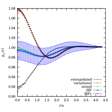
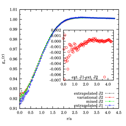
Figure 1: Unlike RDF for the unpolarized fluid of Paziani [16] at $r_{s}=1$ and $\mu=1$ with $162$ particles. On the left panel the calculation with the Jastrow ${\cal J}_{1}$ with various measures: variational histogram (variational) and variational HFv (HFv), mixed histogram (mixed) and HF (HF), and extrapolated histogram (extrapolated). On the right panel the calculation with the Jastrow ${\cal J}_{2}$ with the histogram variational (variational ${\cal J}_{2}$), mixed (mixed ${\cal J}_{2}$), and extrapolated (extrapolated ${\cal J}_{2}$) measures. Also the extrapolated measure with the Jastrow ${\cal J}_{2}$ is compared with the extrapolated measure with the Jastrow ${\cal J}_{1}$. In the inset is shown the difference between the histogram extrapolated measure of the calculation with ${\cal J}_{1}$ and the histogram extrapolated measure of the calculation with ${\cal J}_{2}$. $10^{5}$ Monte Carlo steps were used in the simulations.

Table 1: Contact values for the unlike RDF of the unpolarized fluid of Paziani [16] at various $r_{s}$ and $\mu$ from the mixed measure of the histogram estimator (hist) and the HF measure (HF) with the auxiliary function chosen as in Eq. (5), also reported are the two extrapolated measures (ext and HF-ext). The trial wave function used was of the Slater-Jastrow type with the Jastrow of Ref. [21], ${\cal J}_{2}$. The last column gives the error on the HF measure. $162$ particles were used with $10^{5}$ Monte Carlo steps.

$r_{s}$	$\mu$	hist	ext	HF	HF-ext	$\sigma_{\rm av}$ on HF
10	1/2	1.000(4)	0.91(1)	1.00	0.92	0.03
10	1	0.644(3)	0.582(8)	0.65	0.59	0.03
10	2	0.182(1)	0.146(4)	0.18	0.14	0.06
10	4	0.0506(8)	0.048(2)	0.05	0.04	0.07
10	$\infty$	0.0096(3)	0.0118(8)	0.00	0.00	0.09
5	1/2	1.034(3)	0.94(1)	1.03	0.94	0.03
5	1	0.796(3)	0.743(9)	0.79	0.73	0.02
5	2	0.405(2)	0.362(6)	0.40	0.36	0.02
5	4	0.199(1)	0.184(4)	0.20	0.18	0.03
5	$\infty$	0.0799(8)	0.080(2)	0.06	0.06	0.03
2	1/2	1.0618(4)	0.97(1)	1.05	0.95	0.04
2	1	0.927(3)	0.852(9)	0.93	0.86	0.03
2	2	0.697(3)	0.639(9)	0.69	0.63	0.02
2	4	0.511(2)	0.473(7)	0.51	0.47	0.02
2	$\infty$	0.349(2)	0.323(5)	0.32	0.30	0.02
1	1/2	1.077(3)	0.98(1)	1.07	0.97	0.02
1	1	0.994(3)	0.91(1)	0.99	0.91	0.02
1	2	0.855(3)	0.787(9)	0.86	0.81	0.02
1	4	0.730(2)	0.676(8)	0.73	0.66	0.01
1	$\infty$	0.602(2)	0.560(7)	0.58	0.53	0.01

In conclusions we defined a Hellmann and Feynman estimator to measure a given physical property either in a variational Monte Carlo experiment and in a diffusion Monte Carlo experiment. Our definition coincides with the one of Ref. [13] in the variational case but is different in the diffusion case. We proof tested our definitions on the calculation of the radial distribution function of a particular Fermion fluid. Our simulations showed that the bias is correctly accounted for in both kind of experiments but the variance increases in the diffusion experiment relative to the one of the histogram estimator. We believe it is still an open problem the one of determining the relationship between the choice of the auxiliary function and the variance of the Hellmann and Feynman measure.

The idea for the work came from discussions with Saverio Moroni. I would also like to acknowledge the hospitality of the National Institute for Theoretical Physics (NITheP) of South Africa where the work was done. The simulations were carried out at the Center for High Performance Computing (CHPC), CSIR Campus, 15 Lower Hope St., Rosebank, Cape Town, South Africa.

References

- W. L. McMillan [1965] W. L. McMillan, Phys. Rev. A 138 (1965) 442.
- M. H. Kalos, D. Levesque, and L. Verlet [1974] M. H. Kalos, D. Levesque, and L. Verlet, Phys. Rev. A 9 (1974) 2178.
- Hockney and Eastwood [1981] R. W. Hockney, J. W. Eastwood, ”Computer Simulation Using Particles”, McGraw-Hill, 1981.
- Allen and Tildesley [1987] M. P. Allen, D. J. Tildesley, Computer Simulation of Liquids, Clarendon Press, Oxford, 1987.
- D. Frenkel and B. Smit [1996] D. Frenkel and B. Smit, Understanding Molecular Simulation, Academic Press, San Diego, 1996.
- D. M. Ceperley [1995] D. M. Ceperley, Rev. Mod. Phys. 67 (1995) 279.
- Ceperley [1991] D. M. Ceperley, J. Stat. Phys. 63 (1991) 1237.
- D. M. Ceperley and M. H. Kalos [1979] D. M. Ceperley and M. H. Kalos, in: K. Binder (Ed.), Monte Carlo Methods in Statistical Physics, Springer-Verlag, Heidelberg, 1979, p. 145.
- K. S. Liu, M. H. Kalos, and G. V. Chester [1974] K. S. Liu, M. H. Kalos, and G. V. Chester, Phys. Rev. A 10 (1974) 303.
- R. N. Barnett, P. J. Reynolds, and W. A. Lester, Jr. [1991] R. N. Barnett, P. J. Reynolds, and W. A. Lester, Jr., J. Comp. Phys. 96 (1991) 258.
- S. Baroni and S. Moroni [1999] S. Baroni and S. Moroni, Phys. Rev. Lett. 82 (1999) 4745.
- C. J. Umrigar, M. P. Nightingale, and K. J. Runge [1993] C. J. Umrigar, M. P. Nightingale, and K. J. Runge, J. Chem. Phys. 99 (1993) 2865.
- R. Assaraf and M. Caffarel [2003] R. Assaraf and M. Caffarel, J. Chem. Phys. 119 (2003) 10536.
- R. Gaudoin and J. M. Pitarke [2007] R. Gaudoin and J. M. Pitarke, Phys. Rev. Lett. 99 (2007) 126406.
- L. D. Landau and E. M. Lifshitz [1977] L. D. Landau and E. M. Lifshitz, Quantum Mechanics. Non-relativistic Theory, volume 3, Pergamon Press, third edition, 1977. Course of Theoretical Physics. Eq. (11.16).
- S. Paziani, S. Moroni, P. Gori-Giorgi, and G. B. Bachelet [2006] S. Paziani, S. Moroni, P. Gori-Giorgi, and G. B. Bachelet, Phys. Rev. B 73 (2006) 155111.
- J. Toulouse, R. Assaraf, and C. J. Umrigar [2007] J. Toulouse, R. Assaraf, and C. J. Umrigar, J. Chem. Phys. 126 (2007) 244112.
- A. Bijl [1940] A. Bijl, Physica 7 (1940) 869.
- R. B. Dingle [1949] R. B. Dingle, Philos. Mag. 40 (1949) 573.
- R. Jastrow [1955] R. Jastrow, Phys. Rev. 98 (1955) 1479.
- D. M. Ceperley [2004] D. M. Ceperley, in: G. F. Giuliani and G. Vignale (Ed.), Proceedings of the International School of Physics Enrico Fermi, IOS Press, Amsterdam, 2004, pp. 3–42. Course CLVII.
- D. Ceperley [1978] D. Ceperley, Phys. Rev. B 18 (1978) 3126.