Ising-like transitions in the O($n$) loop model on the square lattice

Abstract

We explore the phase diagram of the O($n$) loop model on the square lattice in the $(x,n)$ plane, where $x$ is the weight of a lattice edge covered by a loop. These results are based on transfer-matrix calculations and finite-size scaling. We express the correlation length associated with the staggered loop density in the transfer-matrix eigenvalues. The finite-size data for this correlation length, combined with the scaling formula, reveal the location of critical lines in the diagram. For $n>>2$ we find Ising-like phase transitions associated with the onset of a checkerboard-like ordering of the elementary loops, i.e., the smallest possible loops, with the size of an elementary face, which cover precisely one half of the faces of the square lattice at the maximum loop density. In this respect, the ordered state resembles that of the hard-square lattice gas with nearest-neighbor exclusion, and the finiteness of $n$ represents a softening of its particle-particle potentials. We also determine critical points in the range $-2\leq n\leq 2$. It is found that the topology of the phase diagram depends on the set of allowed vertices of the loop model. Depending on the choice of this set, the $n>2$ transition may continue into the dense phase of the $n\leq 2$ loop model, or continue as a line of $n\leq 2$ O($n$) multicritical points.

I Introduction

The O($n$) loop model is a highly useful tool for the analysis of O($n$) symmetric $n$-component spin models Stanley ; Domea , and also for that of polymers deG ; Np ; DS . A number of such loop models in two dimensions is exactly solvable N ; Baxter ; BNW ; 3WBN ; 3WPSN ; VF ; S ; PS ; GNB . The present work investigates the nonintersecting loop model described by the partition sum

$$Z_{{\rm loop}}=\sum_{{\rm all}\;{\mathcal{G}}}x^{N_{x}}y^{N_{y}}z^{N_{z}}n^{N_{l}},$$ (1)

where ${\mathcal{G}}$ is a graph consisting of any number of $N_{l}$ closed, nonintersecting loops. Each lattice edge may be covered by at most one loop segment, and there can be 0, 2 , or 4 incoming loop segments at a vertex. In the latter case, they can be connected in two different ways without having intersections. The allowed four kinds of vertices configurations are shown in Fig. 1, together with their weights denoted $x$, $y$ and $z$. The numbers of vertices with these weights are denoted $N_{x}$, $N_{y}$, $N_{z}$ respectively.

This loop model is equivalent with an O($n$) spin model, as described by Ref. BN . The $n$-component spins are sitting in the middle of the edges of the square lattice. The Boltzmann weight for each spin configuration is the product over all vertices of the lattice of the local weights $w$

$$w = 1+x(\vec{s}_{1}\cdot\vec{s}_{2}+\vec{s}_{2}\cdot\vec{s}_{3}+\vec{s}_{3}\cdot\vec{s}_{4}+\vec{s}_{4}\cdot\vec{s}_{1})+y(\vec{s}_{1}\cdot\vec{s}_{3}+\vec{s}_{2}\cdot\vec{s}_{4})$$ (2)

$$+z[(\vec{s}_{1}\cdot\vec{s}_{2})(\vec{s}_{3}\cdot\vec{s}_{4})+(\vec{s}_{2}\cdot\vec{s}_{3})(\vec{s}_{4}\cdot\vec{s}_{1})],$$

where the spins $\vec{s}_{1}$ to $\vec{s}_{4}$ sit on the four edges incident to the vertex and are labeled anticlockwise. The spins are subject to a measure and normalization

$$\int d{\vec{s}}_{k}=1\,,~{}~{}~{}~{}~{}\int d{\vec{s}}_{k}(\vec{s}_{k}\cdot\vec{s}_{k})=n\,.$$ (3)

Expansion of the partition integral in powers of the coupling constants $x,y$ and $z$ turns the spin model into the loop model of Eq. (1).

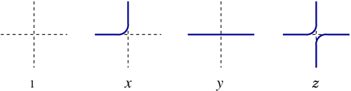
Figure 1: (Color online) The four kinds of vertices of the O($n$) loop model on the square lattice, together with their weights. Rotated versions have the same weights. The present work is restricted to two subspaces of $(x,y,z)$, namely $y=x$, $z=x^{2}$ and $y=0$, $z=x^{2}$.

Although the spin dimensionality $n$ can assume only integer values $n=1,~{}2,~{}\cdots$ in the original O($n$) spin model, $n$ can also have noninteger and even negative values in the loop model of Eq. (1), while the partition sum remains well-defined. Whereas the Boltzmann weight of Eq. (2) can become negative when $x$, $y$ and/or $\sqrt{z}$ exceeds values of order $1/n$, the Boltzmann weights of the loop model remain physical for all non-negative values of $x$, $y$, $z$ and $n$.

The parameter space of Eq. (1) contains several exactly solved “branches” BNW ; 3WBN . These solutions have shown the existence of a richness of phase behavior and “nonuniversal” lines as a function of the vertex weights and $n$ in the range $n<2$. Branches 1 and 2 describe the universal properties of the O($n$) critical point and the low-temperature dense loop phase. Branch 4 describes the superposition of the low-temperature phase and an Ising-like transition where a twofold symmetry of the loop configurations is broken, and branch 3 describes the multicritical point where the Ising-like line in the $(x,z)$ (for constant $y/x$) diagram merges with the O($n$) critical line BN . One can visualize the Ising-like degrees of freedom by assigning $+$ and $-$ spins to the faces of the square lattice, according to the rule that nearest-neighboring spins are equal only if there is a loop segment in between.

Our present aim is to supplement these findings with an analysis of the model of Eq. (1), which has not been solved for general $n$, and with particular attention to the range $n>2$ where we expect an Ising-like transition line. This expectation is based on the observation that, in the limit of large $n$, the local weights are maximal for configurations with small loops on the elementary faces of the lattice. At most one half of these faces can be covered by a loop. There exist two checkerboard-like configurations at maximum covering, similar to the ordered phase of the hard-square model with nearest-neighbor exclusion. We may thus expect a transition for sufficiently large $x$ in the Ising universality class. Since we have set $z=x^{2}$, there is, except for the nearest-neighbor exclusion, no further interaction between the hard squares in the limit $n\to\infty$.

The present work will focus on two subspaces parametrized by $n$ and the bond weight $x$, with $y=x,z=x^{2}$ and $y=0,z=x^{2}$. For large $n$, we expect only small loops, and similar behavior in both cases. However, for small $n$ larger loops exist with, if $y\neq 0$, straight segments due to the $y$-type vertices. As explained in Ref. BN , these $y$-type vertices are responsible for the flipping of an Ising-like degree of freedom along the loops. Thus, for small $n$ we may expect qualitative differences between the cases $y=x$ and $y=0$.

In Sec. II we sketch our numerical procedures used to locate the phase transition lines in the phase diagram. Section III presents the analysis of these numerical results, as well as the resulting phase diagram. The conclusions are summarized and discussed in Sec. IV.

II The transfer-matrix analysis

Our analysis is based on the numerical transfer matrix (TM) calculation of $Z_{\rm loop}$ for $L\times\infty$ square lattices wrapped on a cylinder with circumference $L$. The transfer matrix keeps track of the change of the numbers of loops and the four kinds of vertices when a new layer of $L$ sites is added. The TM techniques for the O($n$) loop model and the procedure for the sparse-matrix decomposition are already described in the literature, e.g., see Ref. BN .

The largest eigenvalue $\Lambda_{0}$ of the TM determines the free energy density $f(L)$ by

$$f(L)=\frac{\ln(\Lambda_{0})}{L}\,.$$ (4)

Its finite-size-scaling behavior at the critical point determines the conformal anomaly $c$ according to BCN ; Aff

$$f(L)\simeq f(\infty)+\frac{\pi c}{6L^{2}}+\cdots\,.$$ (5)

The magnetic correlation function of the O($n$) spin model over a distance $r$ can be expressed in terms of the probability that two vertices at this distance are connected by a single loop segment CG . Thus one may write

$$g_{m}(r)=\frac{Z^{\prime}}{Z}\,,$$ (6)

where $Z^{\prime}$ is the same as in Eq. (1), but with the sum on all loop configurations ${\mathcal{G}}^{\prime}$ that contain one additional single loop segment that runs from position 0 to $r$.

The exponential decay of $g_{m}(r)$ at large distances is determined by the magnetic correlation length $\xi_{h}(x,n,L)$, which can be obtained numerically as

$$\xi_{h}^{-1}(x,n,L)=\ln\left(\frac{\Lambda_{0}}{\Lambda_{1}}\right)\,,$$ (7)

where $\Lambda_{1}$ is the largest eigenvalues in the “magnetic sector”, which refers to the TM for $Z^{\prime}$, which is based on loop configurations with an additional single loop segment running along the cylinder. The scaled magnetic gap $X_{h}$ is defined as

$$X_{h}(x,n,L)=\frac{L}{2\pi\xi_{h}(x,n,L)}\,.$$ (8)

Its finite-size-scaling behavior JCxi ; FSS near a critical point $x_{c}$ is given by

$$X_{h}(x,n,L)=X_{h}+a(x-x_{c})L^{y_{t}}+bL^{y_{u}}+\cdots\,,$$ (9)

where $X_{h}$ is the magnetic scaling dimension, $y_{t}=2-X_{t}$ the temperature exponent, and $y_{u}$ the leading irrelevant exponent. The amplitudes $a$ and $b$ are nonuniversal quantities.

In general, one expects that two phase transitions may occur in the two-dimensional O($n$) model with $n\leq 2$ on the square lattice when the bond weight is increased BN . The first one is the transition from the dilute loop phase to the low-temperature O($n$) phase, where the loops are densely packed. The size of the longest loop diverges at this transition point. The universal properties of this transition follow from the exact solution BNW ; 3WBN for branch 1, and from the Coulomb gas analysis CG . The results for the conformal anomaly and the magnetic exponent are

$$c = 1-\frac{6(g-1)^{2}}{g}\,,$$

$$X_{h} = 1-\frac{1}{2g}-\frac{3g}{8}\,,$$ (10)

where $g$ is the Coulomb gas coupling, which is related to $n$ by $n=-2\cos(\pi g)$ and $1\leq g\leq 2$. The low-temperature phase is still critical in the sense that the magnetic correlation function decays algebraically in the infinite system. The universal properties of the low-temperature phase are characterized by a conformal anomaly $c^{({\rm LT})}$ and a magnetic scaling dimension $X_{h}^{({\rm LT})}$, which can be obtained from the results BNW ; 3WBN ; CG for branch 2 of the square-lattice loop model. They are still given by Eq. (10) and $n=-2\cos(\pi g)$, but with $0\leq g\leq 1$.

A second transition may occur inside the low-temperature phase, when the loops enter an even denser phase which breaks the Ising-like symmetry of the loop configurations BN . Its universal properties BN ; BNW were derived from the solvable case denoted as branch 4. The magnetic scaling dimension $X_{h}^{({\rm LTI})}$ and the conformal anomaly $c^{({\rm LTI})}$ at this Ising-like transition correspond with a combination of low-temperature O($n$) and Ising-like critical behavior, namely

$$X_{h}^{({\rm LTI})}=X_{h}^{({\rm LT})}+1/8$$ (11)

and

$$c^{({\rm LTI})}=c^{({\rm LT})}+1/2\,.$$ (12)

To analyze the expected transition for $n>2$, which drives the loop gas into a loop “solid” phase with a checkerboard pattern, we introduce the staggered loop density and interpret it as the order parameter. First, we define a face as “occupied” by a loop if it is surrounded by a loop or any odd number of loops. In analogy with the hard-square lattice gas, we also divide the faces of the lattice into “odd” and “even” ones. Then one defines the staggered loop density as the density of the occupied odd faces minus that for the even faces. The staggered lattice gas correlation function is thus

$$g_{s}(r)=\langle\rho_{s}(0)\rho_{s}(r)\rangle\,,$$ (13)

where $\rho_{s}(0)$ and $\rho_{s}(r)$ are the staggered densities at positions $0$ and $r$, respectively. For large $n$, we expect that the dense phase is dominated by configurations of elementary loops covering either the even or the odd faces. Therefore, the staggered correlation function is associated with the leading eigenvector $\vec{v}$ of the TM that is antisymmetric under the operation ${\bf R}$ i.e.,

$$\vec{v}=-{\bf R}\vec{v}\,,$$ (14)

where ${\bf R}$ is the operator that rotates the lattice by one lattice unit about the axis of the cylinder. As a consequence of the Perron-Frobenius theorem, the absolute value of the corresponding TM eigenvalue $\Lambda_{2}$ cannot exceed $\Lambda_{0}$ which is associated with a symmetric eigenvector, at least for $n>0$. We expect that the staggered correlation function scales in a similar way as the magnetic correlation function. Thus we describe the exponential decay of the staggered correlation function along the cylinder by means of the staggered scaled gap, defined as

$$X_{s}(x,n,L)=\frac{L}{2\pi}\ln\left(\frac{\Lambda_{0}}{\Lambda_{2}}\right)\,.$$ (15)

The scaled gap $X_{s}(x,n,L)$ is expected to behave according to Eq. (9), with $X_{h}$ replaced by the staggered lattice gas scaling dimension $X_{s}$. This transition breaks the $Z_{2}$ symmetry of odd and even lattice faces, and is thus expected in the Ising universality class: $c=1/2$ and $X_{s}=1/8$.

The critical point can be estimated by numerically solving $x$ in the scaling equation involving two different system sizes

$$X_{i}(x,n,L)=X_{i}(x,n,L^{\prime}),\ \ (i=h,s)\,,$$ (16)

of which the solution $x_{c}(L)$ scales as

$$x_{c}(L)=x_{c}+a^{\prime}L^{y_{u}-y_{t}}+\cdots\,,$$ (17)

where $a^{\prime}$ is an unknown constant. Because $y_{u}<0$ and $y_{t}>0$, $x_{c}(L)$ converges to the critical point $x_{c}$ for a sequence of increasing system sizes $L$. At $x_{c}(L)$, the scaled gap in Eq. (9) converges to the magnetic or the staggered lattice gas scaling dimension $X_{i}(n)$ according to the scaling equation

$$X_{i}(x_{c}(L),n,L)=X_{i}(n)+b^{\prime}L^{y_{u}}+\cdots\,,$$ (18)

with an unknown amplitude $b^{\prime}$. An alternative way to obtain estimates $x_{c}(L)$ of the critical point is to neglect the correction term and thus to solve for $x$ in the equation

$$X_{i}(x,n,L)=X_{i}(n)\,,$$ (19)

where $X_{i}(n)$ is the theoretical prediction for the pertinent scaling dimension. Such predictions can follow the assumption that Eq. (10) or the Ising magnetic scaling dimension $1/8$ applies. If this assumption is correct, the solutions of Eq. (19) converge to the critical point $x_{c}$ as described by Eq. (17). If the assumption is not correct, then the finite-size dependence of the solutions behaves as $L^{-y_{t}}$, so that they still converge to the critical point for $y_{t}>0$, but relatively slowly. The finite-size dependence of the solutions of Eq. (19) may thus reveal if the assumed value of $X_{h}$ is right.

In the present work, we shall make use of both Eq. (16) and Eq. (19) to determine the critical points. In most of these calculations we restrict the system size to even values, because dense loop configurations do not fit well in odd systems, which thus leads to an even-odd alternation effect.

III Results

In the range $-2\leq n\leq 2$, much is already known about the general properties of the phase diagram of the O($n$) loop model on the square lattice BNW ; BN ; 3WBN ; GBN ; GB . This is not the case for the range $n>2$. In this section we explore the phase diagram as a function of $n$, for two types of loop model described by the single bond weight $x$.

III.1 The subspace $y=x$, $z=x^{2}$

In this subsection we explore the phase diagram for the case that there are no further conditions on the set of allowed vertices, thus with vertex weights $x$, $y=x$ and $z=x^{2}$.

For $n\leq 2$, we estimate $x_{c}$ for the O($n$) critical and the low-temperature branches by extrapolating the solutions $x_{c}(L)$ of Eq. (19) with $X_{h}$ the magnetic scaling dimension of the O($n$) critical branch and the low-temperature branch, respectively. This procedure still leads to convergent results in the case that the temperature field associated with $x$ is irrelevant, but less irrelevant than the other nonzero scaling fields, i.e., the case expected for the LT phase of the O($n$) model with not too small $n$, on the basis of the results for branch 2 3WBN ; BN .

The transfer-matrix calculations were performed for system sizes up to $L=16$ or, in some cases, 18. We then calculated the free energy density $f(L)$ at the estimated $x_{c}$, and obtained the conformal anomaly $c$ by fitting these data according to Eq. (5). The numerical results for $x_{c}$ and $c$ are listed in Tables 1 and 2 respectively. Our numerical estimations of $c$ agree well with the theoretical predictions, except for $n=-2$ where the finite-size data display poor convergence.

Table 1: Numerical results for the critical points $x_{c}(n)$ and conformal anomaly $c(n)$ for the O($n$) critical branch in the range $-2\leq n\leq 2$ in the subspace $y=x,z=x^{2}$. The theoretical values for branch 1 of the conformal anomaly are also listed. Estimated numerical uncertainties in the last decimal place are shown between parentheses.

$n$	$x_{c}(n)$	$c_{\rm num}$	$c_{\rm br1}$
$-$2	0.33732317(2)	$-$1.69(1)	$-$2
$-$1.5	0.3444544(1)	$-$1.009(1)	$-$1.00961
$-$1.0	0.35259515(1)	$-$0.60000(2)	$-$3/5
$-$0.5	0.3620756(1)	$-$0.27901(1)	$-$0.279017
0.0	0.3734237(1)	0	0
0.5	0.38757234(1)	0.25594(1)	0.255949876
1.0	0.406446(2)	0.50000(1)	1/2
1.5	0.4353496(1)	0.74183(2)	0.74184247
1.8	0.4664502(1)	0.89185(1)	0.89185788
1.9	0.484688(1)	0.94432(1)	0.9443219
1.95	0.4988697(1)	0.97151(1)	0.971508
1.98	0.512488(1)	0.98835(1)	0.988346
1.99	0.519766(2)	0.99411(2)	0.994103
2.0	0.5386256(2)	1.00000(1)	1

Table 2: Numerical results for the critical point $x_{c}(n)$ and the conformal anomaly $c(n)$ for the low temperature branch (branch 2) in the range $-2\leq n\leq 2$ in the subspace $y=x,z=x^{2}$. The theoretical predictions of conformal anomaly are also listed. Estimated numerical uncertainties in the last decimal place are shown between parentheses.

$n$	$x_{c}(n)$	$c$ (numerical)	$c$ (theory)
1.99	0.559583(1)	0.99372(2)	0.993716
1.98	0.568975(1)	0.98725(2)	0.987247
1.95	0.58904(1)	0.96714(3)	0.967132
1.9	0.6145(1)	0.93180(1)	0.93179998
1.8	0.657(1)	0.8557(1)	0.855602
1.5	0.72(1)	0.588(1)	0.587572
1.4	0.74(1)	0.485(1)	0.4849998

For the Ising-like transition in the LT dense phase, the numerical results for $x_{c}$ at $n=2$ and $n=1.5$ are extrapolated from the solutions of the finite-size scaling equation (16) for $X_{h}(L)$ with even $L$. For other values of $n$, the critical points $x_{c}$ are extrapolated from the solution of the scaling equation (19), in which $X_{h}$ is taken as $X_{h}^{({\rm LTI})}$, for even system sizes up to $L=16$. The free energy density $f(L)$ at the estimated critical point is then calculated for even system sizes up to $L=16$. A fit of these data thus yields the conformal anomaly $c$, in a good agreement with $c^{({\rm LTI})}$ given in Eq. (12). The numerical results for $x_{c}$ and $c$ are listed in Table 3.

Table 3: Numerical results for the critical points $x_{c}(n)$ and the conformal anomaly $c(n)$ for the Ising-like transition inside the LT dense phase in the subspace $y=x,z=x^{2}$. Estimated numerical uncertainties in the last decimal place are shown in parentheses. The results for $c(n)$ agree well with the with the theoretical predictions $c_{\rm br4}$ for branch 4 of the square O($n$) model.

$n$	$x_{c}(n)$	$c(n)$	$c_{\rm br4}$
$-$1.5	1.580(2)	$-$14.4(4)	$-$13.9612
$-$1.0	1.463(1)	$-$6.51(1)	$-$6.5
$-$0.5	1.38398(1)	$-$3.318(1)	$-$3.31779
0.0	1.3229(1)	$-$1.501(1)	$-$1.5
0.5	1.27287(2)	$-$0.318(3)	$-$0.319736
1.0	1.23019(2)	0.50000(4)	0.5
1.2	1.21468(1)	0.759(2)	0.758346
1.5	1.19282(2)	1.088(1)	1.08757
2.0	1.15943(2)	1.502(2)	1.5

Next, we explore the phase diagram for $n>2$. For relatively large values $(n\geq 8)$, we numerically solved for $x_{c}(L)$ in Eq. (19) with the expected Ising value $X_{s}=1/8$. For $n=3,4,5$, we solved for $x_{c}(L)$ in the scaling equation (16). The critical point $x_{c}$ is then estimated for several values of $n$, according to the scaling behavior given in Eq. (17). We then calculated the free energy density $f(L)$ at the estimated critical points for even system sizes up to $L=18$. ¿From a fit of Eq. (5) to the data, we can thus obtain the conformal anomaly $c$. The best estimates of $x_{c}$ and $c$ are listed in Table 4 for several values of $n>2$. Our estimates of $c$ agree well with the expected value $c=1/2$ for the Ising universality class, at least for large $n$. However, for smaller values of $n$, the estimates of $c$ deviate from 1/2. This may be attributed to strong correction to scaling associated with the expected marginal temperature field at $n=2$.

In the limit $n\to\infty$, only loops of the smallest possible size occur, with the size of an elementary square of the lattice. The model of Eq. (1) then reduces to the lattice gas on the square lattice with nearest-neighbor exclusion and no further interactions. We make use of the existing numerical result $\mu_{c}=1.3340151002774(1)$ for the critical value of the chemical potential of this model GBhsq . By relating the weight of an elementary loop to this chemical potential, which leads to $nx_{c}^{4}=\exp(\mu_{c})$, we obtain the large-$n$ limiting behavior of $x_{c}$.

Table 4: Numerical results for the critical points $x_{c}(n)$ and the conformal anomaly $c(n)$ for the lattice-gas-like phase transitions. Results are shown for the two cases $y=x$ and $y=0$. Estimated numerical uncertainties in the last decimal place are shown in parentheses. The results for $c$ agree well with the expected Ising conformal anomaly $c=1/2$, except for $n=2$ and for some relatively small values of $n$ where poor convergence occurs.

	case $y=x$		case $y=0$
$n$	$x_{c}(n)$	$c(n)$	$x_{c}(n)$	$c(n)$
2	——–	——–	0.784(1)	1.49(2)
3	1.101(2)	2.0(6)	0.809(1)	1.3(2)
4	1.12(2)	1.5(2)	0.800(4)	0.9(3)
5	1.00(2)	1.3(2)	0.787(3)	0.6(3)
8	0.907(2)	0.5(1)	0.746(1)	0.50(1)
10	0.857(3)	0.51(1)	0.7202(1)	0.50(1)
15	0.7716(3)	0.501(3)	0.6696(1)	0.50(1)
20	0.7147(3)	0.500(1)	0.6322(1)	0.50(1)
30	0.64060(1)	0.500(1)	0.5795(2)	0.498(2)
40	0.59240(1)	0.500(1)	0.54318(1)	0.500(2)
50	0.55754(1)	0.500(1)	0.51593(1)	0.500(2)
75	0.4995(1)	0.500(1)	0.46888(1)	0.500(1)
100	0.4622(2)	0.500(1)	0.43760(1)	0.500(1)
200	0.3841(1)	0.500(1)	0.36958(1)	0.500(1)
400	0.32004(1)	0.5001(1)	0.311448(1)	0.5000(1)
800	0.26726(1)	0.5001(1)	0.262179(2)	0.5000(1)
1000	0.25230(1)	0.5001(1)	0.248007(1)	0.5000(1)
10000	0.14033(1)	0.5000(1)	0.139573(1)	0.50000(1)

The phase diagram for $n$ in the range $(-2,\infty)$ is shown in Fig. 2. In order to map the range $-2<n<\infty$ on a finite interval, a $1-8/(n+10)$ scale is chosen along the horizontal axis. The vertical axis shows the temperature-like quantity $W\equiv 1/[x(n+10)^{1/4}]$, which parametrizes the bond weight, while remaining finite in the mentioned interval. The curved line on the left is the O($n$) critical line, and a part of its continuation into the low-temperature O($n$) phase which exists only for $n\leq 2$.

Figure 2: The phase diagram of the O($n$) loop model on the square lattice in the ($n,x$) parameter space. In order to map the range $-2<n<\infty$ on a finite interval, a $1-8/(n+10)$ scale is chosen along the horizontal axis. The vertical axis shows the temperature-like quantity $W$ defined in the text. The curved line on the left is the O($n$) critical line, and a part of its continuation into the low-temperature O($n$) phase which exists only for $n\leq 2$. The vertical dashed line shows the boundary of this phase at $n=2$. The line of lattice-gas-like transitions extends all the way to $n=\infty$, where it ends in a point that is accurately known as described in the text.

III.2 subspace $y=0$, $z=x^{2}$

For $y=0$, there exists an exactly solvable case $x_{c}=z_{c}=1/2$, which is called branch 0 BN . For $n=0$ it describes the $\theta$ point of a collapsing polymer BBN . For other values of $n$, it describes a higher critical point (but not the tricritical point analyzed in Ref. GNB ). Since the present value $z=x^{2}$ is smaller than that for branch 0, we do not expect that the $y=0$, $z=x^{2}$ subspace contains the $n=0$ collapse transition. However, the fact that an Ising degree of freedom is associated with each separate loop implies that a degree of Ising ordering is introduced at the critical points for $n<2$, where the largest loops are expected to diverge. Thus, we may expect that, at least for some values of $n$, transitions occur in a different universality class than that of branch 1. Furthermore it remains to be investigated if the phase diagram displays the same topology as that for the $y\neq 0$ case.

First, we investigate that the lattice-gas-like transition persists in the present subspace with $y=0$. For $n\geq 8$, we solved for $x_{c}$ in the scaling equation Eq. (19), using $X_{s}(L)=1/8$ as the Ising magnetic scaling dimension. For $n=2,3,4,5$, we solved instead the scaling equation Eq. (16) for $X_{s}(L)$. Only even $L$ are used in these calculations. We found that the solutions converge in the way described by Eq. (17), confirming that Eq. (9) applies to $X_{s}(L)$, thus indicating that algebraic decaying of the staggered correlation function occurs in the thermodynamic limit. After extrapolation of the critical points $x_{c}$, we calculated the free energy density $f(L)$ at $x_{c}$ for even system sizes up to $L=18$. A fit of the data according to Eq. (5) then yields the conformal anomaly $c$. The results behave in a way similar to the $y=x$ case: in accurate agreement with Ising universality ($c=1/2$), except for a few relatively small $n$ values. The numerical results for $x_{c}$ and $c$ are included in Table 4.

Next we address the question whether the critical manifold continues into the $n\leq 2$ range and connects to an Ising-dense O($n$) transition. We handle this problem by solving $x_{c}(L)$ in the scaling equation (16), for even system sizes up to $L=18$. For $n<1$, the magnetic scaled gap $X_{h}(L)$ is used in Eq. (16). We find that the solution $x_{c}(L)$ converges with $L$ in the way described by Eq. (17). The estimated critical points are included in the phase diagram in the $(x,n)$ plane shown in Fig. 2. We then calculated the magnetic scaled gaps $X_{h}(L)$ for a sequence of systems with even $L$ up to $18$ at the solutions $x_{c}(L)$. Extrapolation of the gaps according to Eq. (18) yields the scaling dimension $X_{h}$, which is listed in Table 5. These results are, in a limited range, compatible with the known scaling dimension $X_{h}$ of the critical O($n$) transition, but the accuracy is low because of strong corrections to scaling, with the exception of the result at $n=0$.

We also calculated the free energy density at the estimated $x_{c}$. A fit of these data by Eq. (5) then yields estimates of the conformal anomaly $c$ for this transition, which are also listed in Table 5. For most values of $n$ these results do not agree with the known theory for the O($n$) critical line, or with a superposition of O($n$) criticality and Ising behavior.

For small finite systems with $n=-1$, the leading eigenvalue $\Lambda_{0}$ becomes twofold degenerate at $x=1/2$. The same applies to the leading eigenvalue $\Lambda_{1}$ in the odd (magnetic) sector. Moreover, these two pairs of eigenvalues are also equal. On this basis we conjecture that $x_{c}(-1)=1/2$ and $X_{h}(-1)=0$.

For $n\geq 1$, we found no solutions of the scaling equation Eq. (16) for $X_{h}(L)$ with even $L$. The staggered scaled gap $X_{s}(L)$ was used instead to study the possible transition. The scaling equation was solved for a sequence of even systems up to $L=18$. We find that the solutions $x_{c}(L)$ behave in a way consistent with convergence to a critical point $x_{c}$ as described in Eq. (17). The estimated critical points are included in the phase diagram in the $(x,n)$ plane shown in Fig. 2.

Next we calculated the scaled staggered gaps $X_{s}(L)$ for even system sizes up to $L=18$ at the solutions $x_{c}(L)$. The gaps converge to the scaling dimension $X_{s}$ according to Eq. (18). Unfortunately, the convergence of the data is not good except for $n=1$. The results for $X_{s}$ are listed in Table 5. For $n=1$ numerical result for $x_{c}$ agrees with the self-dual value $x=1/\sqrt{2}$ (see Sec. IV for further details), and the latter value was used to estimate the universal quantities for $n=1$.

We also calculated the free energy density for $1\leq n\leq 2$ at the estimated critical bond weight $x_{c}$. ¿From a fit of Eq. (5) to these data, we estimate the conformal anomaly $c$ for this transition, as also listed in Table 5.

Table 5: Numerical results for the critical points $x_{c}(n)$, the conformal anomaly $c(n)$ and scaling dimensions $X_{h}(n)$ and $X_{s}(L)$ for several values of $n$ in the subspace $y=0$. Since solutions of Eq. (16) for $X_{h}$ are absent for $n\geq 1$, the result $X_{h}(1)$ was obtained from a fit of the $X_{h,L}$ data at the self-dual value $x=1/\sqrt{2}$ of the bond weight. The latter value was also used to estimate $X_{s}(1)$ and $c(1)$. It is in accurate agreement with the numerical result obtained by fits to the $X_{s}(L)$ data for $n=1$. Satisfactory finite-size convergence is found only for $n=-1$, 0 and 1. The error margins, shown between parentheses, are difficult to estimate in some cases indicated with a question mark.

$n$	$x_{c}(n)$	$X_{h}(n)$	$c(n)$
$-1.0$	1/2	0	$-$2.00(1)
$-0.8$	0.51229(1)	0.06(2)?	$-$1.115(2)
$-0.7$	0.51889(1)	0.07(2)?	$-$0.92(1)
$-0.5$	0.53317(2)	0.07(1)	$-$0.60(1)
$-0.3$	0.54910(1)	0.09(2)	$-$0.339(1)
0.0	0.57686(2)	0.10417(5)	0
0.3	0.6106(3)	0.10(3)	0.306(1)
0.5	0.637(2)	0.16(4)?	0.506(1)
0.8	0.68(1)	0.21(3)?	0.81(1)
1.0	$1/\sqrt{2}$	0.25000000(5)	1.0000 (1)
$n$	$x_{c}(n)$	$X_{s}(n)$	$c(n)$
1.0	$1/\sqrt{2}$	1.00000000(1)	1.0000 (1)
1.2	0.731(2)	0.81(4)	1.13(2)
1.5	0.755(4)	0.5(2)	1.32(1)
1.7	0.768(2)	0.3(3)	1.41(1)
2.0	0.784(1)	0.1(3)	1.49(2)

IV Discussion

Using a finite-size-scaling analysis of results from transfer-matrix calculations, we have determined the phase diagram of the O($n$) loop model on the square lattice in the $(x,n)$ plane, where $x$ is the weight of a lattice edge covered by a loop. Two subspaces, $y=x$ and $y=0$, were investigated.

For $n>>2$ we find an Ising-like phase transition associated with the onset of a checkerboard-like ordering of the elementary loops. In this respect, the ordered state resembles that of the hard-square lattice gas. For large values of $n$ the critical points shown in Fig. 2 approach the accurately known lattice-gas limit. For the case $y=x$ the data in this figure suggest that this approach happens with a weak cusp-like singularity. This behavior can be explained by the residual presence of loops exceeding the size of an elementary faces. The next-smallest loops cover a rectangle with the size of two faces, and contain two $y$-type vertices, at the expense of an extra weight factor $x^{2}$. The presence of these larger loops thus corresponds with a repulsive potential of order $x^{2}\propto 1/\sqrt{n}$ between next-nearest-neighboring hard squares. In lowest order one then expects a linear dependence of the critical chemical potential of the hard-square model on such a repulsion. Noting that the quantity $W$ shown in Fig. 2 plays the role of this chemical potential, one expects that the critical value of $W$ depends linearly on $1/\sqrt{n}$ for large $n$. This corresponds with a square-root like singularity on the scale used in Fig. 2, which behaves as $1/n$ for large $n$. This explains the weak cusp-like singularity.

The appearance of loops exceeding the size of an elementary square, in particular loops covering two squares, can be interpreted as a softening of the nearest-neighbor repulsion. In this respect, the loop model with $n<\infty$ approaches the experimental situation of monatomic gases adsorbed on the (1,0,0) surface of a cubic crystal better than the hard-square model.

These results are in part similar to those obtained for the large-$n$ loop model on the honeycomb lattice ngt2tr , which behaves as a hard-hexagon model Baxhh , with a phase transition in the three-state Potts universality class. It appears that large-$n$ loop models generically approach the behavior of systems of hard particles, with universal properties that are dependent on the microscopic lattice structure. The universal properties may also depend on the allowed set of vertices. For instance, if we put the vertex weights $y=z=0$ in the loop model on the square lattice, then the corresponding hard-square model is subject not only to nearest-neighbor exclusion, but also to next-nearest-neighbor exclusion. The universal behavior of this system is not Ising-like FBN ; KR .

The question about a possible physical interpretation of this large-$n$ transition of the loop model in the language of the spin model specified by Eq. (2) is answered by substitution of the numerical results $x_{c}$ for the critical point, and the length scale $1/\sqrt{n}$ of the spin vectors in that equation. This shows that the Boltzmann factors of the spin model with $n>2$ can become negative at the phase transition. This exposes the unphysical nature of the lattice-gas-like transition in the language of the spin model.

In Sec. III we have also investigated the critical properties of this O($n$) model in the range $-2\leq n\leq 2$. In the case $x=y$, we found that the lattice-gas-like transition line continues into the low-temperature O($n$) phase. The universal behavior along this part of the transition line is interpreted as a superposition of Ising criticality and dense O($n$) loop model behavior, similar to earlier findings for a related square-lattice O($n$) model. For the special point $n=1$, the O($n$) critical point and the Ising-like transition are dual images of one another. The duality transformation includes the sum on the weights of the two $z$-type vertices, thus leading to a single 4-leg vertex with weight $2z$, and a replacement of the loop segments by empty edges and vice versa. The transformation maps the $x$- and $y$-type vertices on the same type, and interchanges the empty and the $z$-type vertices. The normalization of the weight of the empty vertex to 1 thus reduces $x$ and $y$ by a factor $2z$, and changes $z$ into $1/4z$. The $n=1$ results for the critical points $x_{c}$ found in Tables 1 and 3 satisfy this dual relation with one another.

Also for the case $y=0$, we find that the lattice-gas-like transition line continues into the range $n<2$, but the topology of the ($x,n$) phase diagram is different. It does not enter into the dense O($n$) phase, but continues as a line of critical points separating the disordered phase from the dense O($n$) phase. Our numerical data suggest that its universal properties do not match those of the critical O($n$) line (for most of the range $n<1$), or those of a superposition of Ising and critical O($n$) behavior. Furthermore, our results for the universal quantities differ significantly from those reported for branch 3 of the square O($n$) model BN ; BNW and for the tricritical O($n$) model NGB , at least for most of the range $n<1$. We remark that both branch 3 of the square O($n$) model and our $y=0$ critical line lie relatively close to the higher critical point of branch 0 ($x=z=1/2,~{}y=0$), but for $-1<n<1$ they reside on different sides of branch 0. This allows for the possibility that the $y=0$ critical point although also twofold unstable, is attracted by a different fixed point than branch 3. Unfortunately, the limited accuracy of our numerical data for the $y=0$ line case impedes the further identification of its universal nature in terms of possibly existing exact results.

As already mentioned in Sec. I, there exists an Ising-like degree of freedom that is frozen out along each loop for $y=0$. Thus, for $n=0$, where we allow only a single loop, it plays no role and indeed we find the O(0) or SAW critical behavior. For $n\neq 0$ more loops may appear, whose Ising degree of freedom may differ. But, depending on the weight $z$, neighboring loops will tend to meet at $z$-type vertices, and thus assume the same Ising variable. It may thus be expected that at the $y=0$ O($n$) critical point, where the largest loop diverges, there will also be some ordering of the Ising degrees of freedom, thus allowing universal behavior that is different from that of the generic O($n$) critical point.

For $n=1$, the numerical result for $x_{c}$ agrees, within an error margin of about $10^{-5}$, with the self-dual location $x_{c}(1)=1/\sqrt{2}$. Furthermore, this self-dual point can be mapped on Baxter’s 8-vertex model Baxb , by adding down- or left-pointing arrows on the edges covered by an O($n$) loop, and up- or right-pointing arrows to the empty edges. Since two of the vertex weights are zero, the symmetry relations of the 8-vertex model allow a further mapping on the 6-vertex model, with vertex weights $(a,b,c)=(1/\sqrt{2},1/\sqrt{2},1)$ in the notation used in Ref. Baxb .

Also the conjectured critical point $x_{c}(-1)=1/2$ mentioned in Sec. III.2 can be given a more firm basis. We recall that the weight $z$ is actually redundant for $n=-1$ BN . To see this, consider an arbitrary loop configuration where four loop segments come in at a given vertex. There are two possible ways to connect these segments by a $z$-type vertex, and the numbers of loops closed differ by precisely 1. Taking into account that the loop weight is $-1$, one observes that the two contributions due to the summation on the two $z$-type vertices cancel. Thus, in effect, configurations with $z$-type vertices do not contribute to the partition sum. Therefore, the $n=-1$ point of branch 0 in Ref. BN , namely $x=1/2$, is an exact critical point in our $y=0$ subspace, in spite of the fact that the weight $z$ is different. The results $X_{h}=0$ and $c=-2$ found there agree with the present findings.

- (1) H. E. Stanley, Phys. Rev. Lett. 20, 589 (1968).
- (2) E. Domany, D. Mukamel, B. Nienhuis and A. Schwimmer, Nucl. Phys. B 190 [FS3], 279 (1981).
- (3) P. G. de Gennes, Scaling Concepts in Polymer Physics (Cornell University, Ithaca 1979).
- (4) B. Nienhuis, in Fundamental Problems in Statistical Mechanics VII, edited by H. van Beijeren (Elsevier, Amsterdam 1990), p. 255.
- (5) B. Duplantier and H. Saleur Phys. Rev. Lett. 59, 539 (1987).
- (6) B. Nienhuis, Phys. Rev. Lett. 49, 1062 (1982); J. Stat. Phys. 34, 731 (1984).
- (7) R. J. Baxter, J. Phys. A 19, 2821 (1986); J. Phys. A 20, 5241 (1987).
- (8) M. T. Batchelor, B. Nienhuis and S. O. Warnaar, Phys. Rev. Lett. 62, 2425 (1989).
- (9) S. O. Warnaar, M. T. Batchelor and B. Nienhuis, J. Phys. A 25, 3077 (1992).
- (10) S. O. Warnaar, P. A. Pearce, K. A. Seaton and B. Nienhuis, J. Stat. Phys. 74, 469 (1994).
- (11) V. A. Fateev, Sov. J. Nucl. Phys. 33, 761 (1981).
- (12) C. L. Schultz, Phys. Rev. Lett. 46, 629 (1981).
- (13) J. H. H. Perk and C. L. Schultz, in Proc. RIMS Symposium on Non-Linear Integrable Systems, edited by M. Jimbo and T. Miwa (World Scientific, 1983) p. 135; and in Yang-Baxter Equation in Integrable Systems, edited by M. Jimbo (World Scientific, 1990) p. 326.
- (14) W.-A. Guo, B. Nienhuis and H. W. J. Blöte, Phys. Rev. Lett. 96, 045704 (2006).
- (15) H. W. J. Blöte and B. Nienhuis, J. Phys. A 22, 1415 (1989); B. Nienhuis, Int. J. Mod. Phys. B4, 929 (1990).
- (16) H. W. J. Blöte, J. L. Cardy and M. P. Nightingale, Phys. Rev. Lett. 56, 742 (1986).
- (17) I. Affleck, Phys. Rev. Lett. 56, 746 (1986).
- (18) B. Nienhuis, in Phase Transitions and Critical Phenomena, Vol. 11, eds. C. Domb and J. L. Lebowitz (Academic, London, 1987).
- (19) J. L. Cardy, J. Phys. A 17, L385 (1984).
- (20) For a review, see e.g. M. P. Nightingale in Finite-Size Scaling and Numerical Simulation of Statistical Systems, ed. V. Privman (World Scientific, Singapore 1990).
- (21) W.-A. Guo, H. W. J. Blöte and B. Nienhuis, Int. J. Mod. Phys. C 10, 301 (1999).
- (22) W.-A. Guo and H. W. J Blöte, Phys. Rev. E. 83, 021115 (2011).
- (23) W.-A. Guo and H. W. J. Blöte, Phys. Rev. E 66, 046140 (2002).
- (24) H. W. J. Blöte, M. T. Batchelor and B. Nienhuis, Physica A 251, 95 (1998).
- (25) W.-A. Guo, H. W. J. Blöte and F. Y. Wu, Phys. Rev. Lett. 85, 3874 (2000).
- (26) R. J. Baxter, J. Phys. A 19, 2821 (1986); J. Phys. A 20, 5241 (1987).
- (27) X. M. Feng, H. W. J. Blöte and B. Nienhuis, Phys. Rev. E 83, 061135 (2011).
- (28) K. Ramola, Ph. D. Thesis, Tata Institute of Fundamental Research, Mumbai 400005, India (2012).
- (29) B. Nienhuis, W.-A. Guo and H. W. J. Blöte, Phys. Rev. E 78, 061104 (2008).
- (30) R. J. Baxter, Exactly Solved Models in Statistical Mechanics (Academic, London, 1982).