Quantum probes to assess correlations in a composite system

Abstract

We suggest and demonstrate experimentally a strategy to obtain relevant information about a composite system by only performing measurements on a small and easily accessible part of it, which we call quantum probe. We show in particular how quantitative information about the angular correlations of couples of entangled photons generated by spontaneous parametric down conversion is accessed through the study of the trace distance between two polarization states evolved from different initial conditions. After estimating the optimal polarization states to be used as quantum probe, we provide a detailed analysis of the connection between the increase of the trace distance above its initial value and the amount of angular correlations.

The control of quantum systems plays a basic role in the experimental investigation of the predictions of quantum theory as well as in the development of quantum technologies for applications. Indeed, great attention has been recently payed to engineering the dynamics of quantum systems in order to properly generate, manipulate and exploit significant quantum features Myatt2000 ; Kraus2004 ; Chou2005 ; Verstraete2009 ; Barreiro2011 ; Krauter2011 .

Consider a large quantum system whose full characterization is only partially feasible or requires complex measurement schemes. In such a case, it is crucial to develop effective strategies in order to assess relevant pieces of information about the overall system by only monitoring a small part, which then acts as a probe. A natural procedure is to control the interaction of the small subsystem with the rest of the total system in such a way that the former can encode the information of interest. Here, we provide an explicit example of this strategy in an all-optical setup, where the system under study consists of entangled couples of photons generated by spontaneous parametric down conversion (SPDC) Hong1985 ; Joobeur1994 ; Kwiat1999 ; Gerry2005 . By properly engineering the interaction between polarization and momentum degrees of freedom of the photons via a 1D spatial light modulator (SLM), we can access some information regarding the momentum correlations between the two photons by simply performing visibility measurements on the polarization degrees of freedom.

As specific figure of merit, we exploit the trace distance between polarization states. As we shall see, an increase of the trace distance above its initial value allows to detect some information on momentum correlations, which has moved to the polarization degrees of freedom thanks to the engineered interaction. The trace-distance analysis of quantum dynamics has been recently introduced, leading to important results concerning the non-Markovianity of a quantum dynamics Breuer2009 ; Apollaro2011 ; Liu2011 ; Vacchini2011 ; Breuer2012 ; Smirne2013 , the characterization of the presence of initial correlations between the quantum system and its environment Laine2010b ; Smirne2011 ; Dajka2011 ; Gessner2011 , the relevance of non-local memory effects Laine2012 ; Liu2012 ; Laine2012b and the reservoir engineering in ultracold gases Haikka2011 ; Haikka2012 ; Haikka2013 .

The paper is structured as follows. In the next Section we describe the physical system we are going to investigate and present the details of the experimental apparatus. In Section II we illustrate the trace-distance approach to the dynamics of an open system and present the details of the calculations of its evolution for different angular and polarization states. Section III is devoted to illustrate the experimental results about the optmization of the probe and the link between the behavior of trace distance and the initial correlations in the angular degrees of freedom. Finally, Section IV closes the paper with some concluding remarks.

I The physical system and the experimental apparatus

Our overall system consists of couples of entangled photons generated by SPDC in a two-crystal geometry Kwiat1999 . The couples are detected along two beams, named signal and idler, which are centered around the directions fixed by the phase matching condition. The two-photon state generated by SPDC can be written

$$|\psi\rangle= \int d\omega_{p}d\omega_{s}d\theta_{s}d\theta_{i}A(\omega_{p})\tilde{F}(\Delta k_{\perp}){\mbox{Sinc}}(\Delta k_{\parallel}L/2)$$ (1)

$$\times\left[\cos{\alpha}|{\small{H,\theta_{s},\omega_{s}}}\rangle|{\small{H,\theta_{i},\omega_{p}-\omega_{s}}}\rangle\right.$$

$$\left.+e^{i\Phi(\omega_{p},\theta_{s},\theta_{i})}\sin{\alpha}|{\small{V,\theta_{s},\omega_{s}}}\rangle|{\small{V,\theta_{i},\omega_{p}-\omega_{s}}}\rangle\right],$$

where up to first order in frequency and angle,

$$\Delta k_{\parallel} = -\frac{\omega_{p}^{0}\theta^{0}}{2c}(\theta_{s}+\theta_{i})$$

$$\Delta k_{\perp} = \frac{\omega_{p}^{0}}{2c}(\theta_{s}-\theta_{i})+\frac{2\theta^{0}\omega_{s}}{c}.$$ (2)

Here, $\omega_{p}$ is the shift of the pump frequency with respect to the central frequency $\omega^{0}_{p}(405nm)$, $\theta_{s}$ and $\omega_{s}$ ($\theta_{i}$ and $\omega_{i}=\omega_{p}-\omega_{s}$) are the signal (idler) angle and frequency shift with respect to the phase matching condition, $\theta_{s}^{0}=\theta_{i}^{0}\equiv\theta^{0}=3^{\circ}$ and $\omega^{0}_{s}=\omega^{0}_{i}=\omega^{0}_{p}/2$, while $|{\small{P,\theta,\omega}}\rangle$ denotes the single-photon state with polarization ${\small{P=H,V}}$, angle $\theta$ and frequency $\omega$. Moreover, $A(\omega_{p})$ is the spectral amplitude of the pump, $\tilde{F}(\Delta k_{\perp})$ is the Fourier transform of its spatial amplitude and the ${\mbox{Sinc}}(\Delta k_{\parallel}L/2)$ function arises due to the finite crystal size ($L=1mm$) along the longitudinal direction. The two-crystal geometry implies that the polarization degrees of freedom of the two photons are entangled and it further introduces the phase term $\Phi(\omega_{p},\theta_{s},\theta_{i})$, which is due to the different optical paths followed by the couples of photons generated in the first and in the second crystal Rangarajan2009 ; Cialdi2010a ; Cialdi2012 . To first order this term reads $\Phi(\omega_{p},\theta_{s},\theta_{i})\approx\Phi_{0}+\Delta\tau\omega_{p}+\kappa\theta_{s}+\eta\theta_{i}$. Finally, the probabilities of generating $|{\hbox{\small VV}}\rangle$ or $|{\hbox{\small HH}}\rangle$ photons, $\sin^{2}{\alpha}$ and $\cos^{2}{\alpha}$ respectively, are determined by the polarization of the incident laser.

The overall state in Eq.(1) fixes in particular the correlations between signal and idler angular degrees of freedom. By properly engineering the two-photon evolution, relevant information about these angular correlations gets encoded into the polarization degrees of freedom and then can be easily accessed. In fact, through the SLM we can impose an arbitrary polarization- and position-dependent phase shift to the two-photon state in Eq.(1). On the one hand, a linear phase $\overline{\Phi}\equiv-\Phi_{0}-\kappa\theta_{s}-\eta\theta_{i}$ is set to offset the corresponding terms in the first-order expansion of $\Phi(\omega_{p},\theta_{s},\theta_{i})$ Rangarajan2009 ; Cialdi2010a ; Cialdi2012 ; Cialdi2010b . On the other hand, a further linear phase on both signal and idler beams emulates a time evolution of the two-photon state Cialdi2011 .

The experimental setup is shown in Fig. 1. A linearly polarized cw 405 nm diode laser (Newport LQC405-40P) passes through two cylindrical lenses, which compensate beam astigmatism (AC), then through a spatial filter (SF) composed by two lenses and a pin-hole in the Fourier plane to obtain a Gaussian profile by removing the multimode spatial structure of the laser pump. Finally, a telescopic system (TS) prepares a beam with the proper radius and divergence. A couple of 1 mm beta-barium borate crystals (C), cut for type-I downconversion, with optical axis aligned in perpendicular planes, are used as a source of polarization and momentum entangled photon pairs with $\theta^{0}=3^{\circ}$. We use a compensation crystal on the pump (DC) Cialdi2008 , which acts on the delay time between the vertical and horizontal polarization, and a couple of thin crystals ($0.5mm$) for the spatial walk-off compensation (WO). An interference filter or a long pass filter (F) is put on the signal path to select the spectral width of the radiation (10nm or 45nm). In order to obtain different spectral widths or a particular spectral profile, we use a 4f optical system after the coupler on the signal path. The 4f system consists of two gratings (G1 and G2) of $1200lines/mm$ and two achromatic lenses (L1 and L2) with $f=35mm$. The distance between the lenses and the grating is $f$ and the distance between the two lenses is 2f. In this configuration, in between the two lenses the spectral components are focalized and well separated, so that it is possible to put here a slit to select the wanted spectral width. An SLM, which is a liquid crystal phase mask $(64\times 10mm)$ divided in 640 horizontal pixels each $d=100\mu m$ wide, is set before the detectors, at 310 mm from the generating crystals, in order to introduce the spatial phase function. When the mirror (M) is switched on the radiation path a cylindrical lens (L) generates the Fourier Transform profile of the pump at his focal distance (1m), where a CCD camera is located. A couple of polarizer (P) is used to measure the visibility of the entangled state.

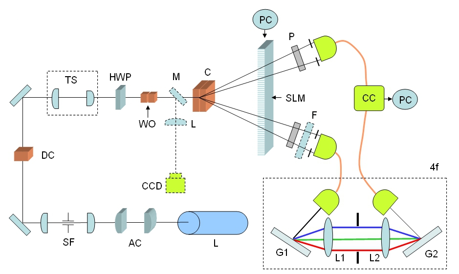
Figure 1: (Color online) Schematic diagram of the experimental setup, as described in Sect.I.

II Trace-distance analysis

II.1 General strategy

The trace distance between two quantum states $\rho^{1}$ and $\rho^{2}$ is defined as

$$D(\rho^{1},\rho^{2})=\frac{1}{2}\mbox{Tr}\left|\rho^{1}-\rho^{2}\right|=\frac{1}{2}\sum_{k}|x_{k}|,$$ (3)

with $x_{k}$ eigenvalues of the traceless operator $\rho^{1}-\rho^{2}$, and it is a metric on the space of physical states such that it holds $0\leq D(\rho^{1},\rho^{2})\leq 1$. The physical meaning of the trace distance lies in the fact that it measures the distinguishability between two quantum states Fuchs1999 . As a consequence, given an open quantum system $S$ interacting with an environment $E$ Breuer2002 , any variation of the trace distance of two open system’s states $D(\rho^{1}_{\scriptscriptstyle S}(t),\rho^{2}_{\scriptscriptstyle S}(t))$ can be read in terms of an exchange of information between the open system and the environment Breuer2009 ; Laine2010b ; Breuer2012 . Here, $\rho^{1}_{\scriptscriptstyle S}(t)$ and $\rho^{2}_{\scriptscriptstyle S}(t)$ are open system’s states evolved from different initial total states $\rho^{1}_{\scriptscriptstyle S\!E}(0)$ and $\rho^{2}_{\scriptscriptstyle S\!E}(0)$ through the relation $\rho^{k}_{\scriptscriptstyle S}(t)=\mbox{tr}_{\scriptscriptstyle E}\left\{U(t)\rho^{k}_{\scriptscriptstyle S\!E}(0)U^{{\dagger}}(t)\right\}$, $k=1,2$, where the total system $SE$ is assumed to be closed and hence evolves through a unitary dynamics $U(t)$ Breuer2002 . In particular, if there are no initial system-environment correlations, $\rho^{1}_{\scriptscriptstyle S\!E}(0)=\rho^{1}_{\scriptscriptstyle S}(0)\otimes\rho^{1}_{\scriptscriptstyle E}(0)$ and $\rho^{2}_{\scriptscriptstyle S\!E}(0)=\rho^{2}_{\scriptscriptstyle S}(0)\otimes\rho^{2}_{\scriptscriptstyle E}(0)$, an increase of the trace distance above its initial value,

$$D(\rho^{1}_{\scriptscriptstyle S}(t),\rho^{2}_{\scriptscriptstyle S}(t))>D(\rho^{1}_{\scriptscriptstyle S}(0),\rho^{2}_{\scriptscriptstyle S}(0)),$$ (4)

witnesses the difference of the two initial environmental states, i.e. $\rho^{1}_{\scriptscriptstyle E}(0)\neq\rho^{2}_{\scriptscriptstyle E}(0)$ Laine2010b ; Smirne2010 . This relation already shows how the trace distance between open system’s states allows to access nontrivial information regarding the environment. More specifically, in the following we present a quantitative link between the trace distance behavior and the environmental correlations.

In view of the trace-distance analysis, our physical system can be characterized as follows. The polarization degrees of freedom are the open system $S$ and the angular degrees of freedom the corresponding environment $E$. The latter are in turn manipulated by varying the divergence of the pump, as well as by selecting the frequency-spectrum width of the two-photon state generated by SPDC. We therefore study the evolution of the trace distance between two polarization states evolved from different initial $SE$ states, which can be considered product states thanks to the compensation of the phase term introduced by the SLM. In particular, we investigate how the trace-distance evolution of the polarization degrees of freedom, which are a small and easily accessible component of the total system, is sensitive to the different angular correlations within $\rho^{1}_{\scriptscriptstyle E}$ and $\rho^{2}_{\scriptscriptstyle E}$, thus allowing to assess this characteristic feature of the overall two-photon state. A logical scheme of the experiment is depicted in Fig.2.

Let us emphasize that our apparatus exploits all the degrees of freedom of the photons generated by SPDC: polarization degrees of freedom as the open system, angles as the environment and frequencies, together with the spatial properties of the pump, as a tool to vary the correlations within the environment.

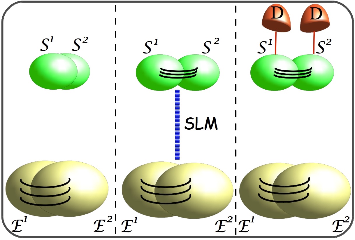
Figure 2: (Color online) Logical scheme of the experiment. In the first stage system and environment are uncorrelated, and the environmental states ($E^{1}$ and $E^{2}$) differ due to correlations. The wiring represents the information about these different correlations. In the second stage system and environment are coupled through the SLM, so that information on the environmental correlations is transferred to the couple of system states ($S^{1}$ and $S^{2}$), making them more distinguishable, and it is finally read out through the detector (D) acting on the system only, in the third and final stage. Note that the two states refer to two distinct runs of the experiment.

II.2 Trace distance evolution for different angular and polarization states

In our apparatus, the angular state after the compensation of the phase through the SLM can be described, setting $\bm{\theta}\equiv(\theta_{s},\theta_{i})$, as

$$\rho_{\scriptscriptstyle E}=\int d\bm{\theta}d\bm{\theta}^{\prime}h(\bm{\theta};\bm{\theta}^{\prime})|\small{\bm{\theta}}\rangle\langle\small{\bm{\theta}^{\prime}}|,$$ (5)

with

$$h(\bm{\theta};\bm{\theta}^{\prime})\equiv{\mbox{Sinc}}(\bm{\theta}){\mbox{Sinc}}(\bm{\theta}^{\prime})\int_{\Omega_{s}}d\omega_{s}\tilde{F}(\Delta k_{\perp})\tilde{F}^{*}(\Delta k_{\perp}^{\prime}).$$ (6)

The influence of the pump spectrum on the angular state can be neglected Cialdi2010a ; Cialdi2010b and the integration over $\omega_{s}$ is performed on the frequency interval $\Omega_{s}$ selected by the filter or the $4f$ setup on the signal path. The joint probability distribution $P(\bm{\theta})\equiv h(\bm{\theta};\bm{\theta})$ determines the angular correlations, which can be quantified as

$$C=\frac{\langle\theta_{s}\theta_{i}\rangle-\langle\theta_{s}\rangle\langle\theta_{i}\rangle}{\sqrt{V_{s}V_{i}}},$$ (7)

with $V_{j}=\langle\theta^{2}_{j}\rangle-\langle\theta_{j}\rangle^{2}$ variance of the angular distribution $P(\theta_{j})$, $j=s,i$. In particular, given a collimated beam with a large pump waist, so that the transverse momentum is nearly conserved, the signal and idler angles are the more correlated the less the selected frequency spectrum is wide. On a similar footing, for a $10nm$-spectrum and a fixed pump waist, the correlation of the angular degrees of freedom grows with decreasing pump divergence. Thus, we can control the initial correlations of the environment by selecting the frequency spectrum of the two-photon state or the divergence of the pump.

The polarization state after the purification trough the SLM reads

$$\rho_{\scriptscriptstyle S}=\gamma|\psi\rangle\langle\psi|+(1-\gamma)\rho^{m},$$ (8)

where

$$|\psi\rangle=\cos{\alpha}|{\hbox{\small HH}}\rangle+\sin{\alpha}|{\hbox{\small VV}}\rangle,$$ (9)

see Eq.(1), is a pure state and $\rho^{m}=\cos^{2}{\alpha}|{\hbox{\small HH}}\rangle\langle{\hbox{\small HH}}|+\sin^{2}{\alpha}|{\hbox{\small VV}}\rangle\langle{\hbox{\small VV}}|$ the corresponding mixture. In our setting, we can control $\alpha$ via the polarization of the pump, while $\gamma$ can be modified by changing the crystal along the pump which precompensates the delay time due to the two-crystal geometry Cialdi2008 . The purity $p=\mbox{Tr}\rho_{\scriptscriptstyle S}^{2}$ of $\rho_{\scriptscriptstyle S}$ is

$$p=1-\frac{1}{2}(1-\gamma^{2})\sin^{2}(2\alpha),$$ (10)

whereas its concurrence $\mathcal{C}$ Wootters1997 reads

$$\mathcal{C}=\gamma|\sin(2\alpha)|.$$ (11)

In the following, we will compare the evolution of polarization states evolved from different initial states $\rho^{k}_{\scriptscriptstyle S}(0)\otimes\rho^{k}_{\scriptscriptstyle E}(0)$, $k=1,2$. The two initial open system’s states $\rho^{k}_{\scriptscriptstyle S}(0)$ have polarization parameters $\alpha_{k}$ and $\gamma_{k}$, see Eqs.(8) and (9), while the two initial environmental states $\rho^{k}_{\scriptscriptstyle E}(0)$ have angular amplitudes $h_{k}(\bm{\theta};\bm{\theta}^{\prime})$, see Eqs.(5) and (6), and then joint angular probability distributions $P_{k}(\bm{\theta})=h_{k}(\bm{\theta};\bm{\theta})$. In particular, we impose through the SLM a linear phase which can be described through the unitary operators

$$U(\beta)|{\small{V\theta_{s}}}\rangle|{\small{V\theta_{i}}}\rangle=e^{i\beta(\theta_{s}-\theta_{i})}|{\small{V\theta_{s}}}\rangle|{\small{V\theta_{i}}}\rangle,$$ (12)

where $\beta$ is the evolution parameter. The polarization states for a generic value of $\beta$ are then

$$\rho^{k}_{\scriptscriptstyle S}(\beta)=\frac{\epsilon_{k}(\beta)}{\sin(2\alpha_{k})}|\psi_{k}\rangle\langle\psi_{k}|+\left(1-\frac{\epsilon_{k}(\beta)}{\sin(2\alpha_{k})}\right)\rho^{m}_{k},$$ (13)

where $|\psi_{k}\rangle=\cos{\alpha_{k}}|{\hbox{\small HH}}\rangle+\sin{\alpha_{k}}|{\hbox{\small VV}}\rangle$ and

$$\epsilon_{k}(\beta)=\gamma_{k}\sin(2\alpha_{k})\int d\theta_{s}d\theta_{i}e^{i\beta(\theta_{s}-\theta_{i})}P_{k}(\theta_{s},\theta_{i}),$$ (14)

which is a real function of $\beta$ since the joint probability distribution is symmetric under the exchange $\theta_{s}\leftrightarrow\theta_{i}$. It is worth emphasizing that the absolute value of $\epsilon_{k}(\beta)$ equals the concurrence as well as the interferometric visibility of the state $\rho^{k}_{\scriptscriptstyle S}(\beta)$. In particular, we measure the visibility by counting the coincidences with polarizers set at $45^{\circ},45^{\circ}$ and at $45^{\circ},-45^{\circ}$, see Cialdi2009 for further details. Moreover, by virtue of the specific evolution obtained through the SLM, $\epsilon_{k}(\beta)$ is fixed by the Fourier transform of the spatial profile $|\tilde{F}(\Delta k_{\perp})|^{2}$, which at first order is a function of $\theta_{s}-\theta_{i}$ and $\omega_{s}$, see Eq.(2), thus depending on both the pump divergence and the selected frequency spectrum. Thus the engineered evolution, see Eq.(12), guarantees that the interferometric visibility is sensitive to the different angular correlations in the environment.

Finally, the trace distance $D(\beta)\equiv D(\rho^{1}_{\scriptscriptstyle S}(\beta),\rho^{2}_{\scriptscriptstyle S}(\beta))$ between the polarization states is simply given by, see Eqs. (3) and (13),

$$D(\beta)=\sqrt{(\cos^{2}\alpha_{1}-\cos^{2}\alpha_{2})^{2}+\left(\epsilon_{1}(\beta)-\epsilon_{2}(\beta)\right)^{2}/4}.$$ (15)

III Experimental results

III.1 Characterization of the probe

As a first step, we show how the choice of the initial polarization states, $\rho^{1}_{\scriptscriptstyle S}(0)$ and $\rho^{2}_{\scriptscriptstyle S}(0)$, influences in a critical way whether the subsequent trace-distance evolution is an effective probe of the different angular correlations in the two initial angular states. To this aim, we fix $\rho^{1}_{\scriptscriptstyle E}(0)$ and $\rho^{2}_{\scriptscriptstyle E}(0)$ as the states corresponding to $\Delta\lambda_{1}=45nm$ and $\Delta\lambda_{2}=10nm$, respectively, that is a weakly and a strongly correlated angular state, while we consider different couples of initial polarization states. To this aim we set $\alpha=\pi/4$ for both $\rho^{1}_{\scriptscriptstyle S}(0)$ and $\rho^{2}_{\scriptscriptstyle S}(0)$, and keep $\gamma_{1}$ fixed, while we vary $\gamma_{2}$ by inserting different precompensation crystals. Specifically, we exploit a $3mm$ crystal to fully compensate the delay time $\Delta\tau$ Cialdi2008 , a $1mm$ crystal to partially compensate it and we also consider the case without any precompensation crystal. The experimental data, together with the theoretical prediction obtained by Eq.(15), are shown in Fig.3.(a). For high values of $\gamma_{2}$, the trace distance between polarization states actually satisfies Eq.(4) and then witnesses the different initial conditions in the angular degrees of freedom. The information due to the differences in $\rho^{1}_{\scriptscriptstyle E}(0)$ and $\rho^{2}_{\scriptscriptstyle E}(0)$ flows to the polarization degrees of freedom because of the engineered interaction. Thus, one can access through simple visibility measurements on the open system some information which was initially outside it. On the other hand, the revival of the trace distance above its initial value decreases with the decreasing of $\gamma_{2}$, and for low enough values of $\gamma_{2}$ the trace distance remains below its initial value for the whole evolution. The loss of purity and entanglement due to a decrease of the parameter $\gamma$ in the initial polarization states can prevent the subsequent trace distance from being an effective probe of the different correlations in the angular states.

The relative weight of vertically and horizontally polarized photons generated by SPDC is determined by the parameter $\alpha$, which can be controlled by properly rotating a half-wave plate set on the pump beam. In Fig.3.(b) we report the experimental data and theoretical predictions of the trace-distance behavior for a given value of $\alpha_{1}$ as well as fixed $\gamma_{1}$ and $\gamma_{2}$, while considering different values of $\alpha_{2}$. One can see that, even if the growth of the trace distance above its initial value decreases with the decreasing of $\alpha_{2}$, it is still visible also for a sensible imbalance between vertically and horizontally polarized photons. Indeed, for a fixed $\gamma<1$ the decrease of $\sin(2\alpha)$ in the polarization states $\rho^{k}_{\scriptscriptstyle S}(0)$ corresponds to a decrease of the concurrence, but to an increase of the purity, see Eqs.(10) and (11). Contrary to what happens for a decrease of the parameter $\gamma_{2}$, see Fig.3.(a), the open system always recovers the information initially outside it from the very beginning of its evolution and the trace-distance maximum increases with the increasing of the initial distinguishability between the two polarization states.

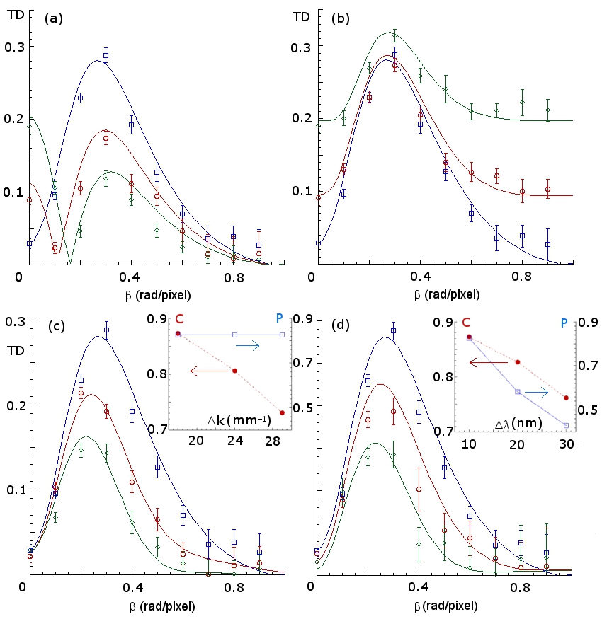
Figure 3: (Color online) Trace distance $D(\beta)$ versus the evolution parameter $\beta$ for different couples of initial system states and different environmental correlations, see Eq.(7), showing how the trace-distance growth is sensitive to the environmental correlations. (a) and (b): $\rho^{1}_{\scriptscriptstyle E}(0)$ and $\rho^{2}_{\scriptscriptstyle E}(0)$ are kept fixed ($\Delta k_{1}=\Delta k_{2}=18mm^{-1}$, $\Delta\lambda_{1}=45nm$ and $\Delta\lambda_{2}=10nm$), $\rho^{1}_{\scriptscriptstyle S}(0)$ is fixed with $\alpha_{1}=\pi/4$ and $\gamma_{1}=0.91$ (mainly due to contributions to the phase in Eq.(1) which are not compensated to the first order), $\rho^{2}_{\scriptscriptstyle S}(0)$ corresponds to $\alpha_{2}=\pi/4$ and $\gamma_{2}=0.96$ (blue line), $0.73$ (red line), $0.52$ (green line) in (a), while $\gamma_{2}=0.96$ and $\alpha_{2}=\pi/4$ (blue line), $0.675$ (red line), $0.575$ (green line) in (b). (c) and (d): $\rho^{1}_{\scriptscriptstyle S}(0)$ and $\rho^{2}_{\scriptscriptstyle S}(0)$ are fixed ($\alpha_{1}=\alpha_{2}=\pi/4$, $\gamma_{1}=0.91$ and $\gamma_{2}=0.96$), $\rho^{1}_{\scriptscriptstyle E}(0)$ is fixed with $\Delta\lambda_{1}=45nm$ and $\Delta k_{1}=18mm^{-1}$, while $\rho^{2}_{\scriptscriptstyle E}(0)$ corresponds to $\Delta\lambda_{2}=10nm$ and $\Delta k_{2}=18mm^{-1}$ (blue line), $24mm^{-1}$ (red line), $29mm^{-1}$ (green line) in (c) and to $\Delta k_{2}=18mm^{-1}$ and $\Delta\lambda_{2}=10nm$ (blue line), $20nm$ (red line), $30nm$ (green line) in (d). The insets in (c) and (d) show the angular correlations (red line) and the purity (blue line) of $\rho^{2}_{\scriptscriptstyle E}(0)$ as a function of $\Delta k_{2}$ (in (c)) or $\Delta\lambda_{2}$ (in (d)). Experimental data are reported with their error bars, the solid lines represent the theoretical predictions.

III.2 Trace distance as a witness of initial correlations in the angular degrees of freedom

The analysis of the previous paragraph shows that the optimal probe of the angular correlations is achieved by exploiting the highest amount of purity and entanglement of the polarization degrees of freedom available within our setting. Now, we study how this optimal probe reveals changes in the angular correlations. Hence, we fix $\rho^{1}_{\scriptscriptstyle S}(0)$, $\rho^{2}_{\scriptscriptstyle S}(0)$ and we investigate the trace-distance evolution $D(\rho^{1}_{\scriptscriptstyle S}(\beta),\rho^{2}_{\scriptscriptstyle S}(\beta))$ for different couples of initial angular states. In particular, we take as reference environmental state $\rho^{1}_{\scriptscriptstyle E}(0)$ the state with weak angular correlations, which is obtained by means of a collimated beam and a $45nm$-spectrum. We compare the evolution of the subsequent polarization state $\rho^{1}_{{\scriptscriptstyle S}}(\beta)$ with the evolution of a state $\rho^{2}_{\scriptscriptstyle S}(\beta)$ evolved in the presence of strong initial angular correlations in $\rho^{2}_{\scriptscriptstyle E}(0)$. We repeat this procedure by changing the amount of correlations $C$ in $\rho^{2}_{\scriptscriptstyle E}(0)$, see Eq.(7), thus studying the connection between $C$ and the effectiveness of the quantum probe of the angular correlations quantified by the increase of the trace distance above its initial value.

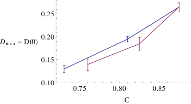
Figure 4: (Color online) Experimental values of the maximum increase of the trace distance above its initial value as a function of the angular correlations $C$, see Eq.(7). The experimental data are referred to the behavior of the trace distance for different beam divergences (blue line, compare with Fig.3.(c)) or different widths of the frequency spectrum (red line, compare with Fig.3.(d)).

In Fig.3.(c), one can see the experimental data and theoretical prediction concerning the different trace-distance evolutions $D(\rho^{1}_{\scriptscriptstyle S}(\beta),\rho^{2}_{\scriptscriptstyle S}(\beta))$ which correspond to the different beam divergences exploited, together with a $10nm$-spectrum, in the preparation of the environmental state $\rho^{2}_{{\scriptscriptstyle E}}(0)$. The divergence is enlarged by suitably setting a telescopic system of lenses, so that the FWHM $\Delta k$ of $|\tilde{F}(\Delta k_{\perp})|^{2}$ is increased, while the $220\mu m$ spot on the generating crystals is kept fixed Cialdi2012 . The increase of the trace distance above its initial value grows with the angular correlations $C$ in $\rho^{2}_{{\scriptscriptstyle E}}(0)$. The behavior of $D(\rho^{1}_{\scriptscriptstyle S}(\beta),\rho^{2}_{\scriptscriptstyle S}(\beta))$ indicates that, for the specific choice of $\rho^{1}_{\scriptscriptstyle S}(0)$ and $\rho^{2}_{\scriptscriptstyle S}(0)$, the trace distance can actually witness even a small difference in the angular correlations of $\rho^{1}_{\scriptscriptstyle E}(0)$ and $\rho^{2}_{\scriptscriptstyle E}(0)$. The direct connection between the trace distance and the correlations in the environment is further shown in Fig.4, where the difference between the maximum and the initial value of the trace distance is plotted as a function of the angular correlations. The experimental data point out that the probe represented by the trace distance is sensitive to the different amount of correlations within the environment, which is indeed not a priori entailed by Eq.(4).

As a further check of the connection between angular correlations and the increase of the trace distance above its initial value, we take into account environmental states $\rho^{2}_{\scriptscriptstyle E}(0)$ in which the angular correlations are modified by selecting different frequency spectra of the two-photon state. Besides affecting the angular correlations, this also influences the purity of $\rho^{2}_{\scriptscriptstyle E}(0)$. As it may be inferred from Eqs.(5) and (6), a wider frequency spectrum implies a lower angular purity, as a consequence of the fact that the pure state generated by SPDC in Eq.(1) also involves the frequencies. However, the trace-distance evolution does not keep track of the purity of the environmental state. In particular, the growth of the trace distance above its initial value is not affected by the different purities of $\rho^{2}_{\scriptscriptstyle E}(0)$ in the two situations, but is determined by the amount of angular correlations $C$, see the insets in Fig.3.(c), (d) and Fig.4. Indeed, this can be explained through Eqs.(14) and (15): the trace distance solely depends on the angular probability distribution $P(\theta_{s},\theta_{i})$, while it is independent of angular coherences.

IV Conclusion

We have theoretically described and experimentally demonstrated a strategy to assess relevant information about a composite system by only observing a small and easily accessible part of it. By exploiting couples of entangled photons generated by SPDC and engineering a proper interaction by means of a SLM, we could reveal correlations within the angular degrees of freedom of the photons by monitoring the trace distance evolution between couples of polarization states. After estimating the optimal probe, we have shown that the increase of the trace distance between system states above its initial value provides a signature of the amount of angular correlations in the environmental states.

- (1) C.J. Myatt, B. E. King, Q.A. Turchette, C.A. Sackett, D. Kielpinski, W.M. Itano, C. Monroe, and D.J. Wineland, Nature 403, 269 (2000)
- (2) B. Kraus and J. I. Cirac, Phys. Rev. Lett. 92, 013602 (2004)
- (3) C.W. Chou, H. de Riedmatten, D. Felinto, S.V. Polyakov, S.J. van Enk, and H.J. Kimble, Nature 438, 828 (2005)
- (4) F. Verstraete, M. M. Wolf, and J. I. Cirac, Nature Phys. 5, 633 (2009)
- (5) J.T. Barreiro, M. Müller, P. Schindler, D. Nigg, T. Monz, M. Chwalla, M. Hennrich, C.F. Roos, P. Zoller, and R. Blatt, Nature 470, 486 (2011)
- (6) H. Krauter, C.A. Muschik, K. Jensen, W. Wasilewski, J.M. Petersen, J.I. Cirac, and E.S. Polzik, Phys. Rev. Lett. 107, 080503 (2011)
- (7) C.K. Hong and L. Mandel, Phys. Rev. A 31,2409 (1985)
- (8) A. Joobeur, B.E.A. Saleh, and M.C. Teich, Phys. Rev. A 50, 3349 (1994)
- (9) P.G. Kwiat, E. Waks, A.G. White, I. Appelbaum, and P.H. Eberhard, Phys. Rev. A 60, R773 (1999)
- (10) C.C. Gerry and P.L. Knight, Introductory Quantum Optics (Cambridge University Press, Cambridge, 2005)
- (11) H.-P. Breuer, E.-M. Laine, and J. Piilo, Phys. Rev. Lett. 103, 210401 (2009); E.-M. Laine, J. Piilo, and H.-P. Breuer, Phys. Rev. A 81, 062115 (2010)
- (12) T.J.G. Apollaro, C. Di Franco, F. Plastina, and M. Paternostro, Phys. Rev. A 83, 032103 (2011)
- (13) B.H. Liu, L. Li, Y.-F. Huang, C.-F. Li, G.-C. Guo, E.-M. Laine, H.-P. Breuer, and J. Piilo, Nature Phys. 7, 931 (2011)
- (14) B. Vacchini, A. Smirne, E.-M. Laine, J. Piilo, and H.-P. Breuer, New. J. Phys. 13, 093004 (2011)
- (15) H.-P. Breuer, J.Phys. B: At. Mol. Opt. Phys. 45, 15 (2012)
- (16) A. Smirne, L. Mazzola, M. Paternostro, and B. Vacchini, arXiv:1302.2055 (2013)
- (17) E.-M. Laine, J. Piilo, and H.-P. Breuer, Europhys. Lett. 92, 60010 (2010)
- (18) A. Smirne, D. Brivio, S. Cialdi, B. Vacchini, and M. G. A. Paris, Phys. Rev. A 84, 032112 (2011)
- (19) J. Dajka, J. Łuczka, and P. Hänggi, Phys. Rev. A 84, 032120 (2011)
- (20) M. Gessner and H.-P. Breuer, Phys. Rev. Lett. 107, 180402 (2011)
- (21) E.-M. Laine, H.-P. Breuer, J. Piilo, C.-F. Li, G.-C. Guo, Phys. Rev. Lett. 108, 210402 (2012)
- (22) B.H. Liu, D.-Y. Cao, Y.-F. Huang, C.-F. Li, G.-C. Guo, H.-P. Breuer, E.-M. Laine, and J. Piilo, arXiv:1208.1358 (2012)
- (23) E.-M. Laine, H.-P. Breuer and J. Piilo, arXiv:1210.8266 (2012)
- (24) P. Haikka, S. McEndoo, G. De Chiara, G. M. Palma, and S. Maniscalco, Phys. Rev. A 84, 031602(R) (2011)
- (25) P. Haikka, J. Goold, S. McEndoo, F. Plastina, and S. Maniscalco, Phys. Rev. A 85, 060101(R) (2012)
- (26) P. Haikka, S. McEndoo, and S. Maniscalco, Phys. Rev. A 87, 012127 (2013)
- (27) R. Rangarajan, M. Goggin, and P. Kwiat, Opt. Exp. 17, 18920 (2009)
- (28) S. Cialdi, D. Brivio, and M.G.A. Paris, Appl. Phys. Lett. 97, 041108 (2010)
- (29) S. Cialdi, D. Brivio, A. Tabacchini, A.M. Kadhim, and M.G.A. Paris, Opt. Lett. 37, 3951 (2012)
- (30) S. Cialdi, D. Brivio, and M.G.A. Paris, Phys. Rev. A 81, 042322 (2010)
- (31) S. Cialdi, D. Brivio, E. Tesio, and M.G.A. Paris, Phys. Rev. A 83, 042308 (2011)
- (32) S. Cialdi, F. Castelli, I. Boscolo, and M.G.A. Paris, Appl. Opt. 47, 1832 (2008)
- (33) C. A. Fuchs, J. van de Graaf, IEEE Trans. Inf. Th. 45, 1216 (1999)
- (34) H.-P. Breuer and F. Petruccione, The Theory of Open Quantum Systems (Oxford University Press, Oxford, 2002)
- (35) A.Smirne, H.P. Breuer, J. Piilo, and B. Vacchini, Phys. Rev. A 82, 062114 (2010)
- (36) S. Hill and W. K. Wootters, Phys. Rev. Lett. 78, 5022 (1997)
- (37) S. Cialdi, F. Castelli, and M.G.A. Paris, J. Mod. Opt. 56, 215 (2009)