Null Phase Curves and Manifolds in Geometric Phase Theory

Abstract

Bargmann invariants and null phase curves are known to be important ingredients in understanding the essential nature of the geometric phase in quantum mechanics. Null phase manifolds in quantum-mechanical ray spaces are submanifolds made up entirely of null phase curves, and so are equally important for geometric phase considerations. It is shown that the complete characterization of null phase manifolds involves both the Riemannian metric structure and the symplectic structure of ray space in equal measure, which thus brings together these two aspects in a natural manner.

1 Introduction

The understanding of the structure and properties of the geometric phase in quantum mechanics, originally discovered in the context of unitary adiabatic cyclic Schrödinger evolution BE , have improved considerably on account of several important later developments. Thus it became clear in successive stages that neither the adiabatic condition nor the cyclic condition are necessary for the existence and identification of the geometric phase SI ; AA . In the latter step, an important role was played by the exploitation of the fact that the state space describing the pure states of a quantum system carries a Riemannian metric, leading to corresponding geodesics in this space. These geodesics were used to convert a general non-cyclic quantum evolution to a cyclic one, so that previous definitions of the geometric phase could then be used to show its existence. The third significant step was the elucidation of a purely kinematical approach to the geometric phase in which the Schrödinger equation and a hermitian hamiltonian operator were both shown to be inessential SB

Several precursors to the quantum-mechanical geometric phase concept have been recognized. Of these, it may be argued that the work of Pancharatnam MS1 in the context of interference phenomena in classical polarization optics, and of Bargmann in the context of the Wigner unitary-antiunitary theorem for symmetry operations in quantum mechanics PA , are particularly significant. Pancharatnam’s work has led to the fruitful concept of two quantum-mechanical Hilbert space vectors being in phase with respect to one another, and more generally to a measure of their relative phase. The phase found by him in polarization optics has been seen later to be an early manifestation of the geometric phase in a decidedly non-adiabatic though cyclic situation.

Bargmann’s work introduced a family of complex expressions into quantum bechanics, later given the name “Bargmann invariants”, which capture in powerful and elegant terms the essential role of complex numbers in the mathematical formalism of quantum mechanics. One of the outcomes of the kinematical approach to geometric phases has been to bring out the importance of the Bargmann invariants, and another has been to combine them with the geodesics mentioned earlier to show that their phases are actually geometric phases for certain cyclic evolutions SB .

The deep interrelations that exist among the ideas of Pancharatnam, Bargmann and Berry have been described elsewhere MUK .

More recently, further exploration of the kinematical treatment of geometric phases has led to the important concept of null phase curves (NPC) in quantum-mechanical Hilbert and ray spaces, which are a vast generalization of geodesics but which preserve the connection between Bargmann invariants and geometric phases RAM . This work has shown that the initial role of geodesics in geometric phase theory has been essentially fortuitous, and that it is the far more numerous NPC’s that really belong to this theory. Indeed, it has been shown that the entire theory can  be built up logically based on Bargmann invariants and NPC’s, with the definition of the latter actually based on the former MAEMM .

Traditional expositions of quantum mechanics  have tended to lay stress on the complex linear structure of Hilbert spaces, the non-commutativity of Hermitian operators representing physical observables, and then drawing out various consequences. In more recent times, with the emphasis given to the study of ray spaces that describe pure quantum states in a one-to-one manner, the rich mathematical structures that come automatically with these spaces have received a great deal of attention EMM . Thus from the familiar complex inner products among Hilbert space vectors there emerge both a Riemannian structure (mentioned above) with a non-degenerate metric on ray space, and a symplectic structure (a classical-looking phase space structure) on the same ray space. Quantum mechanical ray spaces are simultaneously Riemannian manifolds and symplectic manifolds, and this fact would naturally be expected to have important physical manifestations and consequences. The results presented in this work point in that direction.

It has been mentioned that NPC’s are far more numerous than geodesics. This is so to such an extent that it seems reasonable to ask if there are submanifolds (of various dimensions) in quantum-mechanical ray spaces such that every (sufficiently smooth) curve in any one of them is a NPC; and if so, how such submanifolds can be characterized. Such submanifolds have been called Null Phase Manifolds (NPM) and examples given MAEMM . We take up their study here and will show that the characterization of NPM’s indeed involves both the Riemannian structure (through its geodesics) and the symplectic structure of ray space (through the concept of isotropic submanifolds) in equal measure. It is quite remarkable that this should be so, and it suggests that NPM’s are important for grasping the mathematical structure of quantum mechanics at the deepest level.

The contents of this paper are arranged as follows. Section $2$ collects basic notations relating to the Hilbert and ray spaces in quantum mechanics, and the definition of Bargmann invariants and geometric phases in the kinematic approach. The role of ray space geodesics in providing a connection between Bargmann invariants and geometric phases is sketched. After introducing the NPC concept, the greatly enlarged nature of this connection is mentioned. Section $3$ begins with a set of basic relations involving Geometric Phases, NPC’s and the symplectic two-form on ray space. The general definition of a NPM in ray space is then given. While it is easy to see that a NPM is necessarily isotropic (with respect to the ray space symplectic structure), the converse is not true. It is then shown by explicit construction that the most general NPM can be characterized as follows: it is a submanifold in an isotropic and totally geodesic submanifold in ray space, though it may not itself be totally geodesic. Section $4$ gives several examples of the construction of Sect. $3$, in addition to a somewhat detailed description of a general NPC. Section $5$ contains some concluding remarks.

2 Bargmann Invariants, Geometric Phases and NPC’s

We begin by recalling basic notations and definitions from previous work. We denote by $\mathcal{H}$ the complex Hilbert space pertaining to some quantum system. Vectors and the inner product are denoted as $\psi,\phi,...$ and $\left(\phi,\psi\right)$ respectively. The unit sphere $\mathcal{B}\subset\mathcal{H}$ and the ray space $\mathcal{R}$ are respectively:

$$\begin{array}[]{c}\mathcal{B}=\left\{\psi\in\mathcal{H}\mid\text{ }\left(\psi,\psi\right)=1\right\}\subset\mathcal{H};\\ \mathcal{R}=\left\{\rho\left(\psi\right)=\psi\psi^{{\dagger}}\mid\text{ }\psi\in\mathcal{B}\right\}\end{array}$$ (1)

The projection: $\pi:\mathcal{B}\rightarrow\mathcal{R}$ maps $\psi$ to $\pi\left(\psi\right)=\rho\left(\psi\right)$, and  $\mathcal{B}$ is a $U\left(1\right)$ principal bundle over $\mathcal{R}$. If $\mathcal{H}$ is of finite complex dimension $N$, the real dimension of $\mathcal{B}\simeq S^{2N-1}$ is $\left(2N-1\right)$, and that of $\mathcal{R}\simeq CP^{N-1}$ is $2\left(N-1\right)$.

In the kinematic approach to the geometric phase theory, three kinds of curves $\mathcal{C}\subset\mathcal{B}$ of varying degrees of smoothness, and their projections $C=\pi\left[\mathcal{C}\right]$, are needed for specific purposes. With monotonic parametrization, we write uniformly in all cases:

$$\begin{array}[]{c}\mathcal{C}=\left\{\psi\left(s\right)\in\mathcal{B}|\text{ }s_{1}\leq s\leq s_{2}\right\}\subset\mathcal{B}\overset{\pi}{\longrightarrow}\\ C=\pi\left[\mathcal{C}\right]=\left\{\rho\left(s\right)=\psi\left(s\right)\psi^{{\dagger}}\left(s\right)\in\mathcal{R}|\text{ }s_{1}\leq s\leq s_{2}\right\}\subset\mathcal{R}\end{array}$$ (2)

For geodesics we require $\mathcal{C}$ to be continuous twice-differentiable with non-orthogonal endpoints. For NPC’s we need $\mathcal{C}$ continuous once-differentiable with every pair of points on $\mathcal{C}$ non-orthogonal. Finally, for geometric phases to exist we need $\mathcal{C}$ continuous, piecewise once-differentiable with non-orthogonal endpoints. We will find that we have the inclusion relations:

$$\text{Geodesics}\subset\mathrm{\text{NPC}^{\prime}s}\subset\text{Curves with geometric phase}$$ (3)

Two non-orthogonal vectors $\psi,\phi\in\mathcal{B}$ are defined to be “in phase” in the Pancharatnam sense if:

$$\left(\phi,\psi\right)=\overline{\left(\psi,\phi\right)}>0$$ (4)

i.e., $\left(\phi,\psi\right)$ is a positive real number. More generally, the phase of $\psi$ with respect to $\phi$ is defined to be $\arg\left(\phi,\psi\right)$.

The lowest order Bargmann invariant (BI) involves three pairwise non-orthogonal vectors $\psi_{1},\psi_{2},\psi_{3}\in\mathcal{B}$ and is the expression (for $\dim\mathcal{H}\geq 2$):

$$\begin{array}[]{c}\Delta_{3}\left(\psi_{1},\psi_{2},\psi_{3}\right)=\left(\psi_{1},\psi_{2}\right)\left(\psi_{2},\psi_{3}\right)\left(\psi_{3},\psi_{1}\right)=\mathrm{Tr}\left(\rho_{1}\rho_{2}\rho_{3}\right)\\ \rho_{j}=\psi_{j}\psi_{j}^{{\dagger}}\in\mathcal{R},\text{ }j=1,2,3.\end{array}$$ (5)

In a straightforward way this can be generalized to the $n$-th order BI $\Delta_{n}\left(\psi_{1},\psi_{2},...,\psi_{n}\right)$, provided successive pairs of vectors are non-orthogonal.

The geometric phase for a curve $C\subset\mathcal{R}$ (of appropriate type) is defined and most easily calculated using any lift $\mathcal{C}\subset\mathcal{B}$ of it, and it is the difference between a total (or Pancharatnam) phase and a dynamical phase:

$$\begin{array}[]{c}\varphi_{g}\left[C\right]=\varphi_{\text{tot}}\left[\mathcal{C}\right]-\varphi_{\text{dyn}}\left[\mathcal{C}\right]\\ \varphi_{\text{tot}}\left[\mathcal{C}\right]=\arg\left(\psi\left(s_{1}\right),\psi\left(s_{2}\right)\right)\\ \varphi_{\text{dyn}}\left[\mathcal{C}\right]=\text{Im}\int_{s_{1}}^{s_{2}}ds\left(\psi\left(s\right),\psi^{\prime}\left(s\right)\right)\end{array}$$ (6)

The original connection between BI’s and geometric phases involved the use of geodesics in $\mathcal{R}$ and their lifts to $\mathcal{B}$. For any $C\subset\mathcal{R}$ (of appropriate type) its length is defined as the non-degenerate functional:

$$L\left[C\right]=\int_{s_{1}}^{s_{2}}ds\left\{\left\|\frac{d\psi\left(s\right)}{ds}\right\|^{2}-\left|\left(\psi\left(s\right),\frac{d\psi\left(s\right)}{ds}\right)\right|^{2}\right\}^{1/2}$$ (7)

and the second-order ordinary differential equation determining geodesics arises from here as the corresponding Euler-Lagrange equation. Solving it one finds that given any two non-orthogonal points $\rho_{1},\rho_{2}\in\mathcal{R}$ and choosing $\psi_{1}\in\pi^{-1}\left(\rho_{1}\right),$ $\psi_{2}\in\pi^{-1}\left(\rho_{2}\right)$ in phase with one another in the Pancharatnam sense, the (shortest) geodesic from $\rho_{1}$ to $\rho_{2}$ possesses the following lift to $\mathcal{B}$:

$$\psi\left(s\right)=\psi_{1}\cos s+\frac{\psi_{2}-\psi_{1}\left(\psi_{1},\psi_{2}\right)}{\sqrt{1-\left(\psi_{1},\psi_{2}\right)^{2}}}\sin s;\text{ }0\leq s\leq\cos^{-1}\left(\psi_{1},\psi_{2}\right)\in\left(0,\pi/2\right)$$ (8)

We see that $\psi\left(s\right)$ is a real (positive) linear combination of $\psi_{1}$ and $\psi_{2}$, and $\psi\left(s\right),\psi\left(s^{\prime}\right)$ are in phase in the Pancharatnam sense for all $s,s^{\prime}$. Then the BI-geometric phase connection is:

$$\arg\Delta_{3}\left(\psi_{1},\psi_{2},\psi_{3}\right)=-\varphi_{g}\left[\text{\text{geodesic triangle in }}\mathcal{R}\text{ \text{with vertices }}\rho_{1},\rho_{2},\rho_{3}\right]$$ (9)

(This easily generalizes to higher-order BI’s). Notice that while the left-hand side depends only on the vertices, the definition of the right-hand side requires that they be connected in some manner, here by geodesics.

Now we come to the definition of a NPC. A curve $C\subset\mathcal{R}$ (of appropriate type), along with any lift $\mathcal{C}\subset\mathcal{B}$, is a NPC if:

$$\Delta_{3}\left(\psi\left(s\right),\psi\left(s^{\prime}\right),\psi\left(s^{\prime\prime}\right)\right)=\overline{\Delta_{3}\left(\psi\left(s\right),\psi\left(s^{\prime}\right),\psi\left(s^{\prime\prime}\right)\right)}>0.\quad\forall s,s^{\prime},s^{\prime\prime}\in\left[s_{1},s_{2}\right].$$ (10)

From Eq.(8) we see that every geodesic is a NPC, but it turns out that for $\dim\mathcal{H}\geq 3$ the converse is not true. The key property of a NPC is that:

$$\varphi_{g}\left[\text{\text{any connected portion of a NPC}}\right]=0$$ (11)

so connected portions of a NPC are themselves NPC’s. This definition is designed just so that in place of the connection (9) we have the vastly extended relation :

$$\begin{array}[]{c}\arg\Delta_{3}\left(\psi_{1},\psi_{2},\psi_{3}\right)=-\varphi_{g}[\text{\text{ ``triangle" in }}\mathcal{R}\text{ \text{with vertices}}\\ \rho_{1},\rho_{2},\rho_{3}\text{ \text{joined pairwise by } NPC}\text{'s}]\end{array}$$ (12)

(This also generalizes to higher orders). Hereafter it will be convenient to denote by $N_{1,2}$ a NPC from $\rho_{1}$ to $\rho_{2}$ in $\mathcal{R}$, and by $\mathcal{N}_{1,2}$ a lift of it to $\mathcal{B}$.

At this point we bring in the basic differential-geometric objects which are important for the following work. The dynamical phase $\varphi_{\text{dyn}}\left[\mathcal{C}\right]$ in Eq.(6) is the integral along $\mathcal{C}$  of a one-form $A$ on $\mathcal{B}$:

$$\varphi_{\text{dyn}}\left[\mathcal{C}\right]=\int_{\mathcal{C}}A\text{ },\text{ \ }A=-i\psi^{{\dagger}}d\psi$$ (13)

This connection one-form is not the pull-back via $\pi^{\ast}$ of any one-form on the ray space $\mathcal{R}$. However, the exterior derivative $dA$, its curvature, is the pull-back of a closed non-degenerate (symplectic) two-form $\omega$ on $\mathcal{R}$:

$$dA=\pi^{\ast}\omega\text{ },\text{ }d\omega=0\text{ },\text{ }\omega\text{ \text{non-degenerate on }}\mathcal{R}$$ (14)

If $\mathcal{S}\subset\mathcal{B}$ is any smooth connected two-dimensional surface with projection $S=\pi\left[\mathcal{S}\right]\subset\mathcal{R}$, we have:

$$\oint_{\partial\mathcal{S}}A=\int_{\mathcal{S}}dA=\int_{S}\omega$$ (15)

As a consequence, if in Eq.(6) we take $C$ to be closed, and its lift $\mathcal{C}$ to be also closed, we find that the geometric phase is a symplectic area. This is, if $\partial C=\emptyset$, $\partial\mathcal{C}=\emptyset$ and $S$ is any surface such that $\partial S=C$, then:

$$\varphi_{g}\left[C\right]=-\varphi_{\text{dyn}}\left[\mathcal{C}\right]=-\oint_{\mathcal{C}}A=-\int_{S}\omega\,.$$ (16)

Explicit forms for $A$ and $\omega$ in local (Darboux) coordinates may be easily obtained.

As mentioned earlier, it has been shown that the entire theory of the geometric phase can be built up starting from BI’s and NPC’s. In this process, the fact that (for $\dim\mathcal{H}\geq 3$) there are infinitely many NPC’s connecting any two non-orthogonal points $\rho_{1},\rho_{2}\in\mathcal{R}$, as against a single geodesic, has led to the concept of NPM’s. The precise definition of a NPM will be given in the next section. At one extreme, a single NPC is an example of a one-dimensional NPM. At the other extreme, for $\mathcal{H}$ of finite dimension, one can ask for the maximum possible dimension of a NPM. It has been shown that a NPM must be an isotropic submanifold in $\mathcal{R}$, bringing in the symplectic structure of $\mathcal{R}$. However it has also been shown that isotropy is not sufficient to obtain the NPM property. This “gap” will be examined, and a complete characterization of NPM’s obtained, in the next section.

3 NPM’s and Isotropic Totally Geodesic Submanifolds.

We begin by assembling a set of background results on geometric phases for general curves in $\mathcal{R}$. As with the notations $N_{1,2}$ and $\mathcal{N}_{1,2}$ for NPC’s, by $C_{1,2}$ we will mean a general curve (of appropriate kind) connecting given $\rho_{1},\rho_{2}\in\mathcal{R}$, and $\mathcal{C}_{1,2}$ a lift of it. The general non-additivity of geometric phases is expressed by:

$$\begin{array}[]{c}\varphi_{g}\left[C_{1,2}\cup C_{2,3}\cup...\cup C_{n-1,n}\right]=\varphi_{g}\left[C_{1,2}\right]+\varphi_{g}\left[C_{2,3}\right]+...+\varphi_{g}\left[C_{n-1,n}\right]\\ -\arg\Delta_{n}\left(\psi_{1},\psi_{2},...,\psi_{n}\right);\text{ }\rho_{j}=\psi_{j}\psi_{j}^{{\dagger}},\text{ }j=1,2,...,n\end{array}$$ (17)

An exception occurs for $n=3$ if we choose $\rho_{3}=\rho_{1}$. Then:

$$\varphi_{g}\left[C_{1,2}\cup C_{2,1}\right]=\varphi_{g}\left[C_{1,2}\right]+\varphi_{g}\left[C_{2,1}\right]$$ (18)

For a curve $C_{1,2}$, let us denote by $\widetilde{C}_{1,2}$ the reversed curve from $\rho_{2}$ to $\rho_{1}$; then the geometric phase changes sign, and from Eq.(18) we get for two curves from $\rho_{1}$ to $\rho_{2}$:

$$\varphi_{g}\left[C_{1,2}^{\prime}\right]=\varphi_{g}\left[C_{1,2}\right]-\varphi_{g}\left[C_{1,2}\cup\widetilde{C}_{1,2}^{\prime}\right]$$ (19)

As the argument of the second term is a closed loop, we can use Eq.(16) to get:

$$\varphi_{g}\left[C_{1,2}^{\prime}\right]=\varphi_{g}\left[C_{1,2}\right]-\int_{S}\omega,\text{ \ }\partial S=C_{1,2}\cup\widetilde{C}_{1,2}^{\prime}$$ (20)

This relation shows how the geometric phase changes if the endpoints are kept fixed and the connecting curve is varied smoothly.

If in Eq.(18) we take $C_{2,1}$ to be a NPC $N_{2,1}$ and then use Eq.(16), we get:

$$\varphi_{g}\left[C_{1,2}\right]=\varphi_{g}\left[C_{1,2}\cup N_{2,1}\right]=\int_{S}\omega,\text{ \ }\partial S=C_{1,2}\cup N_{2,1}$$ (21)

This is the most general way in which the geometric phase for an open curve can be converted to that for a closed loop.

In order to set up the definition of a NPC, we recall how to obtain Eq.(11) from Eq.(10) for a single NPC . Given a NPC $N$, Eq.(10) allows us to construct particular lifts $\mathcal{N}_{0}$ which have the global Pancharatnam property. For a fiducial $\rho_{0}\in N$, we choose $\psi_{0}\in\pi^{-1}\left(\rho_{0}\right)$. Then for each $\rho\in N$, we choose MAEMM ; man $\psi=\rho\psi_{0}/\sqrt{\mathrm{Tr}(\rho\rho_{0})}$ and thus build up $\mathcal{N}_{0}$. Eq.(10) then shows that any two vectors $\psi,\psi^{\prime}\in\mathcal{N}_{0}$ are also in phase in the Pancharatnam sense, so $\mathcal{N}_{0}$ is globally “in phase”. The vanishing of  geometric phases for all connected portions of $N$, Eq.(11), is now immediate. In fact, both total and dynamical phases vanish individually.

The definition of a NPM can now be given in three equivalent ways. Let $M$ be a (regular) simply connected submanifold in $\mathcal{R}$, and write the identification map as usual as: $i_{M}:M\hookrightarrow\mathcal{R}$. Then:

$$\begin{array}[]{c}M\text{ is a NPM}\\ \Leftrightarrow\text{\text{every} }C\subset M\text{ is a NPC}\\ \Leftrightarrow\Delta_{3}\left(\psi_{1},\psi_{2},\psi_{3}\right)=\overline{\Delta_{3}\left(\psi_{1},\psi_{2},\psi_{3}\right)}>0\text{ }\forall\rho_{j}=\psi_{j}\psi_{j}^{{\dagger}}\in M,\text{ }j=1,2,3\\ \Leftrightarrow\text{\text{there exist lifts }}\mathcal{M}_{0}\text{ \text{which are globally `` in phase"}}\end{array}$$ (22)

The third statement follows from the second by a construction similar to the NPC case described above. It is a simple consequence of Eqs.(22) that:

$$\rho_{1},\rho_{2}\in M\Longrightarrow\mathrm{Tr}\left(\rho_{1}\rho_{2}\right)>0$$ (23)

so a NPM does not contain mutually orthogonal points. The isotropy property of $M$ also follows easily:

$$\begin{array}[]{c}C\subset M,\text{ }\partial C=\emptyset,\text{ }C\text{ {a }}NPC\Longrightarrow\\ \int_{S}\omega_{M}=0,\text{ }\forall S\subset M,\text{ with }\partial S=C,\text{ }\omega_{M}=i_{M}^{\ast}\omega\Longrightarrow\omega_{M}=0\end{array}$$ (24)

as there is complete freedom in the choice of the closed loop $C\subset M$. Therefore a NPM is necessarily isotropic.

Now we consider the situation in the reverse direction. For a regular submanifold $M\subset\mathcal{R}$, which obeys the isotropy condition $i_{M}^{\ast}\omega=0$, what additional properties are needed to conclude that $M$ is a NPM? Let us assume hereafter that the $M$ under consideration always obeys Eq.(23). Let the curves $C_{1,2},C_{1,2}^{\prime}$ and the surface $S$ with $\partial S=C_{1,2}\cup\widetilde{C}_{1,2}^{\prime}$ all be chosen to lie within $M$. Then, given $i_{M}^{\ast}\omega=0$, from Eq.(20) we have:

$$\varphi_{g}\left[C_{1,2}^{\prime}\right]=\varphi_{g}\left[C_{1,2}\right]$$ (25)

Therefore $\varphi_{g}\left[C_{1,2}\right]$ is unchanged by continuous changes of the curve which preserve its endpoints; that is, $\varphi_{g}\left[C_{1,2}\right]$ depends only on $\partial C_{1,2}$. This falls short of showing that, for a closed loop $C\subset M$ is such that $\partial S=C$ for a surface $S\subset M$, $\varphi_{g}\left[C\right]$ always vanishes.

If now it is the case that for every pair of points $\rho_{1},\rho_{2}\in M$, the geodesic from $\rho_{1}$ to $\rho_{2}$ lies totally in $M$, then in Eq.(25) we can take $C_{1,2}^{\prime}$ to be this geodesic and then conclude that  $\varphi_{g}\left[C_{1,2}\right]=0$. This would mean that every $C$ is a NPC, and $M$ a NPM.

Actually it is clear that a weaker property of $M$ would suffice: if for  every $\rho_{1},\rho_{2}\in M$ there is at least one NPC $N_{1,2}\subset M$, then again by taking $C_{1,2}^{\prime}=N_{1,2}$ in Eq.(25) we reach the desired conclusion: $\varphi_{g}\left[C_{1,2}\right]=0$ and every $C$ is a NPC. Equally well we can take $N_{1,2}$ in Eq.(21) to be this NPC, and then also by isotropy we get the desired result. However, it would be inappropriate to assume the existence of some NPC’s in the process of proving that all $C$ are NPC’s.

A submanifold $M\subset\mathcal{R}$ (obeying Eq.(23)) with the property that the geodesics connecting pairs of points in $M$ lie totally in $M$ is said to be totally geodesic hel . We have therefore shown that a (regular, simply connected) isotropic totally geodesic submanifold $M\subset\mathcal{R}$ is definitely a NPM. However the converse is not true for a simple reason. In an $M$ which is isotropic and totally geodesic (therefore a NPM) we can choose any regular submanifold $M^{\prime}\subset M$ which will certainly be isotropic as well as a NPM, but will in general not be a totally geodesic submanifold. This gap which remains can be closed by the following argument.

Let us collect the conclusions so far obtained:

$$\begin{array}[]{c}\left(a\right)\text{ }M\text{ is a NPM}\Rightarrow M\text{ \text{is isotropic}}\\ \left(b\right)\text{ }M\text{ \text{ simply connected, isotropic totally geodesic }}\Rightarrow\text{ }M\text{ is a NPM}\\ \left(c\right)\text{ }M^{\prime}\text{ \text{a simply connected regular submanifold in \ an isotropic totally geodesic}}\\ \text{\text{submanifold }}\Longrightarrow M^{\prime}\text{ is a NPM}\end{array}$$ (26)

We now show by construction that (26-c) holds in the reverse direction as well. Dropping primes:

$$\begin{array}[]{c}M\text{ \text{is a NPM}}\Longrightarrow M\text{ \text{ is a regular submanifold in \ an}}\\ \text{\text{isotropic totally geodesic submanifold}}\end{array}$$ (27)

The construction is as follows. Given the NPM  $M\subset\mathcal{R}$, we select one of its lifts $\mathcal{M}_{0}$ which has the Pancharatnam “ in phase” property globally (cfr. Eq.(22)):

$$\begin{array}[]{c}M\subset\mathcal{R,}\text{NPM}\longrightarrow\mathcal{M}_{0}\subset\mathcal{B},\text{ }\pi\left[\mathcal{M}_{0}\right]=M;\\ \psi,\psi^{\prime}\in\mathcal{M}_{0}\Longrightarrow\left(\psi,\psi^{\prime}\right)=\overline{\left(\psi,\psi^{\prime}\right)}>0\end{array}$$ (28)

We pass now from $\mathcal{M}_{0}$ to its non-negative real linear hull, namely $\widetilde{\mathcal{M}}_{0}\subset\mathcal{B}$ made up of all (normalized) real non-negative linear combinations of all sets of vectors in $\mathcal{M}_{0}$, hence $\widetilde{\mathcal{M}}_{0}$ is simply connected. Clearly $\mathcal{M}_{0}\subseteq\widetilde{\mathcal{M}}_{0}$, and $\widetilde{\mathcal{M}}_{0}$ retains the property of isotropy since it is a NPM: because of Eq.(28) and the method of construction of $\widetilde{\mathcal{M}}_{0}$, all total and dynamical phases vanish for curves in $\widetilde{\mathcal{M}}_{0}$. In particular, the second line of (28) remains valid for all pairs of vectors in $\widetilde{\mathcal{M}}_{0}$. Now however $\widetilde{\mathcal{M}}_{0}$ (more precisely $\widetilde{M}=\pi\left[\widetilde{\mathcal{M}}_{0}\right]$) is totally geodesic since the construction in Eq.(8) of geodesics is totally in the real domain. This completes the proof of Eq.(27). $\Box$

It should be clear that we need to resort to this construction or extension $M\rightarrow\widetilde{M}$ only if $M$ is not already totally geodesic. Then it is also clear that the extension involved is minimal.

At this point we can answer the question raised at the end of Sect.2 concerning the maximum possible dimension of a NPM, assuming the dimension $N$ of $\mathcal{H}$ is finite. From the isotropy property it is clear that this maximum is $\left(N-1\right)$, one half of the real dimension of the ray space $\mathcal{R}$. This follows from $\mathcal{R}$ being a symplectic manifold of dimension $2\left(N-1\right)$. Therefore a NPM  $M$ of dimension $\left(N-1\right)$ is in fact a Lagrangian submanifold in $\mathcal{R}$ (i.e., maximal isotropic), and it is necessarily already totally geodesic, since there is no possible extension of $M$ to a larger isotropic submanifold.

4 Illustrative Examples

We now consider some examples of NPM’s, to which for illustrative purposes the construction of the previous Section can be applied. Since a single NPC, being one-dimensional, is the simplest instance of a NPM, we begin with this case.

The definition of a NPC is given in Eq.$\left(\ref{NPC.2.10}\right)$. A more explicit description has been developed in Ref.$\left[9\right]$ and is as follows. Let two distinct non-orthogonal points $\rho_{1},\rho_{2}\in\mathcal{R}$ obeying: $\mathrm{Tr}\left(\rho_{1}\rho_{2}\right)>0$ be given. Let $N\subset\mathcal{R}$ be a NPC from $\rho_{1}$ to $\rho_{2}:$

$$\begin{array}[c]{c}N=\left\{\rho\left(s\right)\in\mathcal{R}|\text{ }s_{1}\leq s\leq s_{2},\text{ }\rho\left(s_{1}\right)=\rho_{1},\text{ }\rho\left(s_{2}\right)=\rho_{2}\right\}\subset\mathcal{R}\\ \mathrm{Tr}\left(\rho\left(s\right)\rho\left(s^{\prime}\right)\rho\left(s^{\prime\prime}\right)\right)=\text{ \text{real positive }}\forall s,s^{\prime},s^{\prime\prime}\in\left[s_{1},s_{2}\right]\end{array}$$ (29)

Choose vectors $\psi_{1},\psi_{2}\in\mathcal{B}$ projecting onto $\rho_{1},\rho_{2}$ respectively, with $\left(\psi_{1},\psi_{2}\right)$ real positive, so that  $\psi_{1}$ and $\psi_{2}$ are in phase in the Pancharatnam sense. As shown in the previous Section, we can construct a lift $\mathcal{N}_{0}$ of $N$ from $\psi_{1}$ to  $\psi_{2}$ which has the global Pancharatnam property:

$$\begin{array}[c]{c}\mathcal{N}_{0}=\left\{\psi_{0}\left(s\right)\in\mathcal{B}|\text{ }s_{1}\leq s\leq s_{2},\text{ }\psi_{0}\left(s_{1}\right)=\psi_{1},\text{ }\psi_{0}\left(s_{2}\right)=\psi_{2};\text{ }\rho\left(s\right)=\pi\left(\psi_{0}\left(s\right)\right)\right\}\subset\mathcal{B}\\ \left(\psi_{0}\left(s\right),\psi_{0}\left(s^{\prime}\right)\right)=\text{ \text{real positive }}\forall s,s^{\prime}\in\left[s_{1},s_{2}\right]\end{array}$$ (30)

We express the endpoints of  $\mathcal{N}_{0}$ as:

$$\begin{array}[c]{c}\psi_{1}=e_{1},\text{ }\psi_{2}=e_{1}\cos\theta_{0}+e_{2}\sin\theta_{0},\text{ }\theta_{0}\in(0,\pi\left.{}\right)\\ \left(e_{i},e_{j}\right)=\delta_{ij},\text{ }i,j=1,2\end{array}$$ (31)

Denote by $\mathcal{H}_{\bot}$ the orthogonal complement in $\mathcal{H}$ to the two-dimensional subspace spanned by $e_{1}$ and $e_{2}$:

$$\mathcal{H}_{\bot}=\left\{\phi\in\mathcal{H}|\text{ }\left(e_{1},\phi\right)=\left(e_{2},\phi\right)=0\right\}$$ (32)

Then the vectors $\psi_{0}\left(s\right)\in\mathcal{N}_{0}$ can be expressed as:

$$\begin{array}[c]{c}\psi_{0}\left(s\right)=x_{1}\left(s\right)e_{1}+x_{2}\left(s\right)e_{2}+\chi\left(s\right)\\ \chi\left(s\right)\in\mathcal{H}_{\bot}\\ \left|x_{1}\left(s\right)\right|^{2}+\left|x_{2}\left(s\right)\right|^{2}+\left(\chi\left(s\right),\chi\left(s\right)\right)=1\end{array}$$ (33)

At $s=s_{1},s_{2}$ we have:

$$\begin{array}[c]{c}x_{1}\left(s_{1}\right)=1,\text{ }x_{2}\left(s_{1}\right)=0,\text{ }\chi\left(s_{1}\right)=0\\ x_{1}\left(s_{2}\right)=\cos\theta_{0},\text{ }x_{2}\left(s_{2}\right)=\sin\theta_{0},\text{ }\chi\left(s_{2}\right)=0\end{array}$$ (34)

If we set $s^{\prime}=s_{1},s_{2}$ in the positivity condition of Eq.(30) we find:

$$x_{1}\left(s\right),\text{ }x_{1}\left(s\right)\cos\theta_{0}+x_{2}\left(s\right)\sin\theta_{0}\text{ \text{real positive }}\forall s\in\left[s_{1},s_{2}\right]$$ (35)

We may therefore replace $x_{1}\left(s\right)$ and $x_{2}\left(s\right)$, which are both real, by the expressions:

$$x_{1}\left(s\right)=\sigma\left(s\right)\cos\theta\left(s\right),\text{ }x_{2}\left(s\right)=\sigma\left(s\right)\sin\theta\left(s\right)$$ (36)

subject to:

$$\begin{array}[c]{c}0<\sigma\left(s\right)\leq 1,\text{ }-\frac{\pi}{2}+\theta_{0}<\theta\left(s\right)<\frac{\pi}{2}\\ \theta\left(s_{1}\right)=0,\text{ }\theta\left(s_{2}\right)=\theta_{0},\text{ }\sigma\left(s_{1}\right)=\sigma\left(s_{2}\right)=1\end{array}$$ (37)

Of course, for a particular NPC  these ranges may not be fully utilized. For the squared norm of $\chi\left(s\right)$ we have:

$$\left\|\chi\left(s\right)\right\|^{2}=\left(\chi\left(s\right),\chi\left(s\right)\right)=1-\sigma\left(s\right)^{2}\geq 0$$ (38)

The remaining content of the positivity condition in Eq.(30) is:

$$\sigma\left(s\right)\sigma\left(s^{\prime}\right)\cos\left(\theta\left(s^{\prime}\right)-\theta\left(s\right)\right)+\left(\chi\left(s^{\prime}\right),\chi\left(s\right)\right)=\text{ \text{real positive }}\forall s^{\prime},s\in\left(s_{1},s_{2}\right)$$ (39)

This leads to $\left(\chi\left(s^{\prime}\right),\chi\left(s\right)\right)$ being real. It can be seen quite easily that as a consequence it should be possible to choose an orthonormal basis $\left(e_{3},e_{4},...\right)$ for  $\mathcal{H}_{\bot}$ such that:

$$\begin{array}[c]{c}\chi\left(s\right)={\displaystyle\sum\limits_{r=3,4,...}}x_{r}\left(s\right)e_{r},\text{ }x_{r}\left(s\right)\text{ \text{real}}\\ \left\|\chi\left(s\right)\right\|^{2}={\displaystyle\sum\limits_{r=3,4,...}}x_{r}\left(s\right)^{2}=1-\sigma\left(s\right)^{2}\in\left[0,1\right)\end{array}$$ (40)

Then $\left(e_{1},e_{2},e_{3},...\right)$ is an orthonormal basis for $\mathcal{H}$, with the choice of $e_{3},e_{4},...$ depending in general on the particular NPC $N$ and lift $\mathcal{N}_{0}$ being considered.

Summarizing, the vectors along the special lift $\mathcal{N}_{0}$ of $N$ are real linear combinations of the basis vectors $\left(e_{1},e_{2},e_{3},...\right)$:

$$\psi_{0}\left(s\right)={\displaystyle\sum\limits_{r=1,2,...}}x_{r}\left(s\right)e_{r}=\sigma\left(s\right)\cos\theta\left(s\right)e_{1}+\sigma\left(s\right)\sin\theta\left(s\right)e_{2}+\chi\left(s\right)$$ (41)

subject to the conditions in Eqs.(34), (37) and (39). While the conditions at $s_{1}$ and $s_{2}$ are easy to state and ensure, the non-local condition (39) has the geometrical meaning that for all $s^{\prime},s\in\left(s_{1},s_{2}\right)$ the real unit vectors $\widehat{x}\left(s^{\prime}\right)=\left\{x_{1}\left(s^{\prime}\right),x_{2}\left(s^{\prime}\right),x_{3}\left(s^{\prime}\right),...\right\}$ and  $\widehat{x}\left(s\right)=\left\{x_{1}\left(s\right),x_{2}\left(s\right),x_{3}\left(s\right),...\right\}$ must make an angle less than $\pi/2$ with each other.

Based on this description of the most general NPC from $\rho_{1}$ to $\rho_{2}$, a relatively simple class of NPC ’s suggests itself. We extend the pair $\left\{e_{1},e_{2}\right\}$ to an orthonormal basis $\left\{e_{1},e_{2},e_{3},...\right\}$ in $\mathcal{H}$ in any way we wish, and choose some $m\in\left\{3,4,...\right\}$. Then $\left\{e_{1},e_{2},...,e_{m}\right\}$ is an orthonormal set in $\mathcal{H}$, and we limit ourselves to vectors $\psi_{0}\left(s\right)\in\text{Sp}\left\{e_{1},e_{2},...,e_{m}\right\}$. Let $\mathbb{S}^{m-1}\subset\mathbb{R}^{m}$ be the real unit sphere in an $m$-dimensional real Euclidean space. Within $\mathbb{S}^{m-1}$, let us choose the region $\mathbb{S}_{+}^{m-1}$ where all $m$ coordinates are positive:

$$\mathbb{S}_{+}^{m-1}=\left\{\widehat{x}=\left(x_{1},x_{2},...,x_{m}\right)\in\mathbb{S}^{m-1}|\text{ }x_{j}>0,\text{ }j=1,2,...,m\right\}\subset\mathbb{S}^{m-1}$$ (42)

Then by choosing once-differentiable $\widehat{x}\left(s\right)\in\mathbb{S}_{+}^{m-1}$ for $s_{1}<s<s_{2}$, with $\widehat{x}\left(s_{1}\right)=\left(1,0,...\right)$ and $\widehat{x}\left(s_{2}\right)=\left(\cos\theta_{0},\sin\theta_{0},0,...\right)$, we generate a NPC $\mathcal{N}_{0}\subset\mathcal{B}$ from $\psi_{1}$ to $\psi_{2}$ as follows:

$$\begin{array}[c]{c}\psi_{0}\left(s\right)={\displaystyle\sum\limits_{r=1.}^{m}}x_{r}\left(s\right)e_{r}\\ \psi_{0}\left(s_{1}\right)=\psi_{1}=e_{1},\text{ }\psi_{0}\left(s_{2}\right)=\psi_{2}=e_{1}\cos\theta_{0}+e_{2}\sin\theta_{0}\end{array}$$ (43)

By construction we have ensured the NPC condition:

$$\left(\psi_{0}\left(s\right),\psi_{0}\left(s^{\prime}\right)\right)=\widehat{x}\left(s\right)\mathbf{\cdot}\,\widehat{x}\left(s^{\prime}\right)>0,\quad\forall s,s^{\prime}\in\left[s_{1},s_{2}\right].$$ (44)

As depicted in the figure, this NPC can be pictured as a once-differentiable curve lying in $\mathbb{S}_{+}^{m-1}$ and running from $\left(1,0,...,0\right)$ to $\left(\cos\theta_{0},\sin\theta_{0},0,...,0\right):$

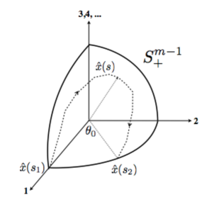
Figure 1: The dotted curve represents a special class of NPC’s pictured on $\mathbb{S}_{+}^{m-1}$.

The passage from the one-dimensional NPC  $\mathcal{N}_{0}=\left\{\psi_{0}\left(s\right)\right\}\subset\mathcal{B}$ to its real non-negative linear hull, in the manner of the previous section, leads to a (generally higher-dimensional) submanifold $\widetilde{\mathcal{M}}_{0}\subset\mathcal{B}$. This construction can be carried out, for instance, by forming all convex linear combinations of all subsets of vectors on $\mathcal{N}_{0}$, and then normalizing the result. In $\mathcal{B}$, and in the image in $\mathbb{S}_{+}^{m-1}$, we have:

$$\begin{array}[c]{c}\psi=c{\displaystyle\sum\limits_{j}}p_{j}\psi_{0}\left(s_{j}\right),\text{ }p_{j}>0,\text{ }{\displaystyle\sum\limits_{j}}p_{j}=1,\text{ }\left\|\psi\right\|=1\\ \widehat{x}=c{\displaystyle\sum\limits_{j}}p_{j}\widehat{x}\left(s_{j}\right),\text{ }\widehat{x}\mathbf{\cdot}\widehat{x}=1\text{\ }\end{array}$$ (45)

The image of  $\widetilde{\mathcal{M}}_{0}$ on $\mathbb{S}_{+}^{m-1}$ is that it is the minimal convex cone containing (the image of) $\mathcal{N}_{0}$. We can see that the arc in the $1-2$ plane from $\widehat{x}\left(s_{1}\right)$ to $\widehat{x}\left(s_{2}\right)$ is included. Going back to $\widetilde{\mathcal{M}}_{0}\subset\mathcal{B}$ and its image $\widetilde{M}=\pi\left(\widetilde{\mathcal{M}}_{0}\right)\subset\mathcal{R}$, it is clear that both isotropy and the totally geodesic property have been achieved in a minimal manner starting from $\mathcal{N}_{0}$.

To deal with the most general NPC (from $\psi_{1}$ to $\psi_{2}$) as described in Eq.(41) subject to Eqs.(35), (37) and (39 ) (and with the limitation to $\mathrm{span}\left\{e_{1},e_{2},e_{3},...,e_{m}\right\}$), we must permit the choice of $e_{3},e_{4},...,e_{m}$ to depend on the particular NPC. Then we see that in the figure above the path of the real unit vector  $\widehat{x}\left(s\right)$ can explore regions of $\mathbb{S}^{m-1}$ outside of  $\mathbb{S}_{+}^{m-1}$, while obeying the non-local positivity condition in Eq.(30). Thus for any $s$ and $s^{\prime}$, the angle between $\widehat{x}\left(s\right)$ and $\widehat{x}\left(s^{\prime}\right)$ must be less than $\pi/2$. The component $x_{1}\left(s\right)>0$ throughout, while $x_{2}\left(s\right),x_{3}\left(s\right),...,x_{m}\left(s\right)$ can each be sometimes negative. However, the image of  $\widetilde{\mathcal{M}}_{0}$ is still the minimal convex cone on $S^{m-1}$ containing the image of $\mathcal{N}_{0}$.

Turning to examples of NPM’s $M\subset\mathcal{R}$ of higher dimensions, we consider two cases from Ref.$\left[9\right]$. The first one, in the  $\mathbb{S}_{+}^{m-1}$ picture just used to discuss single NPC’s, is to take (the global Pancharatnam lift) $\mathcal{M}_{0}$ to be essentially $\ \mathbb{S}_{+}^{m-1}$:

$$\begin{array}[c]{c}\mathcal{M}_{0}=\left\{\psi\left(\widehat{x}\right)={\displaystyle\sum\limits_{r=1}^{m}}x_{r}e_{r}|\text{ }\widehat{x}\in\mathbb{S}_{+}^{m-1}\right\}\subset\mathcal{B}\\ M=\pi\left(\mathcal{M}_{0}\right)\subset\mathcal{R}\end{array}$$ (46)

Since:

$$\left(\psi\left(\widehat{x}\right),\psi\left(\widehat{x}^{\prime}\right)\right)=\widehat{x}\mathbf{\cdot}\widehat{x}^{\prime}=\text{ \text{real }}>0$$ (47)

we have the NPM property for $M$:

$$\Delta_{3}\left(\psi\left(\widehat{x}\right)\psi\left(\widehat{x}^{\prime}\right)\psi\left(\widehat{x}^{\prime\prime}\right)\right)=(\widehat{x}\mathbf{\cdot}\widehat{x}^{\prime})(\widehat{x}^{\prime}\mathbf{\cdot}\widehat{x}^{\prime\prime})(\widehat{x}^{\prime\prime}\mathbf{\cdot}\widehat{x})=\text{ \ \text{real }}>0$$ (48)

In this case, as is also obvious from the definition of $\mathcal{M}_{0}$, its real non-negative linear hull is itself: $\widetilde{\mathcal{M}}_{0}=\mathcal{M}_{0}$, so $M$ is already both isotropic and totally geodesic.

The second more concrete example involves a set of real Schrödinger wave functions in $\mathcal{H}=L^{2}\left(\mathbb{R}^{N}\right)$. We start from the ground-state wave function of the $N$-dimensional isotropic simple harmonic oscillator and and all its spatial translates:

$$\begin{array}[]{c}\psi_{0}\left(\mathbf{x}\right)=\pi^{-N/4}\exp\left(-\mathbf{x\cdot x}/2\right),\text{ }\mathbf{x\cdot x}={\displaystyle\sum\limits_{j=1}^{N}}x_{j}^{2}\\ \psi_{\mathbf{y}}(x)=\psi_{0}(\mathbf{x-y}),\;\mathbf{y}\in\mathbb{R}^{N}\end{array}$$ (49)

All these wave functions are normalized and pointwise real positive, and taken together they define $\mathcal{M}_{0}$:

$$\mathcal{M}_{0}=\left\{\psi_{\mathbf{y}}\left(\mathbf{x}\right)|\text{ }\mathbf{y}\in\mathbb{R}^{N}\right\}\subset\mathcal{B}\subset\mathcal{H}$$ (50)

As all inner products $\left(\psi_{\mathbf{y}},\psi_{\mathbf{y}^{\prime}}\right)$ are trivially real positive, $M=\pi\left(\mathcal{M}_{0}\right)$ is clearly an $N$-dimensional NPM in $\mathcal{R}$. However, on its own, $M$ is not totally geodesic. The extension of $\mathcal{M}_{0}$ to its real non-negative linear hull can be accomplished by first constructing “convex combinations” of the wave functions $\psi_{\mathbf{y}}\left(\mathbf{x}\right)$, namely:

$$\psi\left(\mathbf{x}\right)=c\int p\left(\mathbf{y}\right)\exp[-\left(\mathbf{x}-\mathbf{y}\right)\mathbf{\cdot}\left(\mathbf{x}-\mathbf{y}\right)/2]\,\,d^{N}y,\qquad p\left(\mathbf{y}\right)\geq 0$$ (51)

and then fixing $c$ so that $\psi\left(\mathbf{x}\right)$ is normalized (here we must permit choices of $p\left(\mathbf{y}\right)$ involving Dirac delta functions as well). This process clearly involves a genuine (minimal) enlargement of $\mathcal{M}_{0}$ to $\widetilde{\mathcal{M}}_{0}$, and then the totally geodesic property as well as isotropy is achieved for $\widetilde{M}=\pi\left(\widetilde{\mathcal{M}}_{0}\right)$.

The same reasoning may be applied to the class of Generalized Gaussian states SSM of the kind:

$$\psi_{\mathbf{y},U}\left(\mathbf{x}\right)=\pi^{-N/4}(\det U)^{1/4}\exp\left(-\mathbf{(x-y)}\cdot U\mathbf{(x-y)}/2\right)$$ (52)

where $\mathbf{y}$ is again an $N$-dimensional translation vector while $U$ is a real positive definite symmetric matrix. In this case $M=\pi\left(\mathcal{M}_{0}\right)$ is an $N+N(N+1)/2$-dimensional NPM and the analogue of formula (51) involves also an integral over the $N(N+1)/2$ variables that parametrize the space of real positive definite symmetric matrices, hence yielding a quadratic increase in the dimension of the manifold.

5 Concluding Remarks

It is well appreciated that the concept of the geometric phase belongs to the basic foundations of quantum mechanics. Its study has progressively revealed many important aspects of the mathematical structure of the subject and the interrelations among them. The introduction of the concepts of Bargmann invariants and null phase curves has added considerable richness to the subject.

On the other hand, the unravelling of the basic geometric features of the state or ray spaces of quantum mechanics has been receiving considerable attention EMM . It is quite remarkable that these spaces are simultaneously manifolds with Riemannian metric structures and symplectic structures. The work in this paper has brought these two aspects very close together in the context of the geometric Phase, by showing that null phase manifolds can be fully characterized only by combining these structures suitably. At an elementary level, a null phase manifold in ray space is a submanifold in which all “evolutions” have identically vanishing geometric phases. However, the fact that its understanding needs both the metric and symplectic structures of ray space  is quite remarkable, and can be expected to shed more light on the foundations of quantum mechanics.

Acnowldegments

G.M. would like to acknowledge the support provided by the Santander/UCIIIM University Chair of Exccellence Programme 2011-12.

References

(1) M.V. Berry, Proc. Roy. Soc. A392, 45 (1984).
(2) B. Simon, Phys. Rev. Lett. 51, 2167 (1983).
(3) Y. Aharonov and J. Anandan, Phys. Rev. Lett. 58, 1593 (1987).
(4) J. Samuel and R. Bhandari, Phys. Rev. Lett. 60, 2339 (1988).
(5) N. Mukunda and R. Simon, Ann. Phys. 228, 205 (1993).
(6) S. Pancharatnam, Proc. Ind. Acad. Sci. A44, 247 (1956).
(7)Pancharatnam, Bargmann and Berry phases - A retrospective., N. Mukunda in Quantum Field Theory - A 20th
century profile, Asoke N. Mitra (ed.), Hindustan Book Agency and Indian National Scoenc Academy (2000), p. 324-336.
(8) E.M. Rabei, Arvind, N. Mukunda and R. Simon, Phys. Rev. A60, 3397 (1999).
(9) N. Mukunda, Arvind, E. Ercolessi, G. Marmo, G. Morandi and R. Simon, Phys. Rev. A67, 042114 (2003).
(10) E. Ercolessi, G. Marmo and G. Morandi, La rivista del Nuovo Cimento 33, 401 (2010).
(11) V.I. Man’ko, G. Marmo, E.C.G. Sudarshan and F. Zaccaria, Phys. Lett. A 273, 1525 (2002).
(12) S. Helgason, Differential Geometry, Lie Groups and Symmetric Spaces, Academic Press, San Diego (1978).
(13) R. Simon, E.CG. Sudarshan and N. Mukunda, Phys. Rev. A37, 3028 (1988).