Phase diagram of the quantum $O(2)$-model in $2+1$ dimensions

Abstract

The quantum $O(2)$ model in $2+1$ dimensions is studied by simulating the 3d $O(2)$ model near criticality. Finite densities are introduced by a non-zero chemical potential $\mu$, and the worm algorithm is used to circumvent the sign problem. The renormalisation is discussed in some detail. We find that the onset value of the chemical potential coincides with the mass gap. The $\mu$-dependence of the density rules out Bose-Einstein condensation and might be compatible with an interacting Fermi gas. The $\mu$-$T$ phase diagram is explored using the density and the magnetic susceptibility. In the cold, but dense regime of the phase diagram, we find a superfluid phase.

I Introduction

The $O(2)$-model as a statistical field theory in three dimensions has always enjoyed great phenomenological importance: to name only a few applications, it illuminates the superfluid transition ($\lambda$ -point) of pure ${}^{4}He$ Ahlers (1976), it describes the electromagnetic penetration depth in certain high-$T_{c}$ superconducting materials Kamal et al. (1994) and it might provide insights in the Bose-Einstein condensation of atomic vapour (hard sphere bosons) Grüter et al. (1997). It is well known (see e.g. Gottlob and Hasenbusch (1993)) that the 3d classical theory possesses a second order phase transition at a critical inverse temperature $\beta_{c}=0.45420(2)$ separating the disordered phase at $\beta<\beta_{c}$ from an ordered state for $\beta>\beta_{c}$. In solid state physics, the atomic characteristic length $a$ sets the fundamental scale of the theory. For later use, we introduce the dimensionless correlation length as the physical correlation length in units of the atomic scale, i.e., $\xi_{\mathrm{latt}}(\beta):=\xi/a$. It is this correlation length which diverges at the phase transition.

The $O(2)$-model inherits its name from a global $O(2)$ symmetry, which lets us define a (Noether) current. The generalisation of the $O(2)$-model to include a finite chemical potential, which favours the proliferation of density, has recently attracted a lot of interest: The probabilistic weight is now complex, and the model inhibits the numerical study with classical Monte-Carlo methods based upon importance sampling with respect to a real and positive probabilistic weight. Thus, the model shares this notorious sign problem with the theory of strong interactions, i.e., QCD, at finite baryon densities. The QCD phase diagram as a function of temperature and chemical potential is still not known form first principle calculations, and the prospects are bleak unless a change of paradigm let us address theories with sign problems on more generic grounds. Such breakthroughs might equally well be made in the context of simplistic theories such as the $O(2)$-model at finite densities. Over the recent past, quite some progress has been made in this direction: Monte-Carlo simulations which are based upon importance sampling with respect to the density of states, an always real and positive quantity, might circumvent the sign problem Wang and Landau (2001); Langfeld et al. (2012). The so-called complex Langevin approach Parisi (1983); Karsch and Wyld (1985) is based upon a complexification of the fields and might be ideally suited to address complex action systems. This approach has been largely explored over the recent years Aarts (2009a); Aarts et al. (2010) including the $SU(3)$ spin model at finite densities Aarts and James (2012). Concerns about its reliability have been raised recently, since the approach, although it converges, does not give the correct answer in certain cases. While the Bose gas is a spectacular success story for the complex Langevin approach Aarts (2009a, b), the approach fails to produce the correct answer for a close relative, the $O(2)$-model in certain regions of parameter space Aarts and James (2010). Progress has been made recently by devising criteria for correctness of the method Aarts et al. (2011a, b). Another promising idea, firstly put forward by Chadrasekharan in Chandrasekharan (2008), is based upon a reformulation of the theory in terms of new, potentially non-local variables in a sign-problem free manner. In particular, the so-called world-line or worm algorithm Prokof’ev and Svistunov (2001, 2009) has been identified as an approach with a wide range of applications including theories with sign problems. As pointed out by Gattringer, the so-called $SU(3)$ spin model, which is motivated from dense QCD in the limit of heavy quarks, is accessible by means of worm (also called flux type) algorithms even at finite densities Mercado et al. (2011); Gattringer (2011); Mercado and Gattringer (2012); Gattringer and Schmidt (2012). Most relevant for the study here is the flux representation of the $O(2)$-model Alet and Sørensen (2003a, b). A thorough analysis of the classical model at finite densities has been presented by Chadrasekharan in Banerjee and Chandrasekharan (2010). Finally, the so-called fermion bag approach has recently been put forward in Chandrasekharan (2010); Chandrasekharan and Li (2012) and might have the potential to gain new insights into fermionic theories with sign problems.

Although a range of classical theories with sign-problems have been explored in the recent past, to the best of our knowledge such an investigation of a finite density quantum field theory has not yet been performed. In the present paper, we will bridge this gap and systematically explore the quantum limit of the $O(2)$-model at finite densities. For this purpose, we rely to a large extent on the flux type algorithm Banerjee and Chandrasekharan (2010) which will give us access to the full phase diagram as a function of temperature and chemical potential. Generic quantum phenomena such as superfluidity will be described by a first principle simulation.

On a practical note, the quantum limit of the model is accessible using simulations of the classical theory and by performing a detailed scaling analysis near the critical point. This will then reveal the properties of the quantum $O(2)$ theory in $2+1$ dimensions. Let us explore the correspondence between classical and quantum theory a bit further: In the latter context, the inverse temperature $\beta$ is re-interpreted as the spin-spin coupling strength, and the temperature $T$ is now attained by the extent of the torus in “time” direction. The inverse correlation length is now interpreted as the mass gap, $m=1/\xi$. This mass takes over the role of the fundamental scale of the quantum field theory and is kept fixed under a change of the coupling strength $\beta$. The formerly introduced atomic length $a$ (also called the lattice spacing in the quantum context) merely plays the role of a regulator. This regulator $a$ now necessarily depends on the coupling strength: $m\,a(\beta)=1/\xi_{\mathrm{latt}}(\beta)$. Tuning the coupling $\beta$ to the critical value (at a fixed value for $m$) implies that the lattice spacing tends to zero. This then installs the continuum limit of the quantum theory.

II Model set-up and symmetries

In $2+1$ dimensions, the $O(2)$-model, also called the $xy$-model, is formulated on a cubic grid of size $V=N_{t}N_{x}N_{y}$. Dynamical degrees of freedom are the angles $\phi_{x}$ which are associated with the sites $x$ of the lattice and which parametrise the unit vectors

$$\vec{n}_{x}=\Bigl{(}\cos(\phi_{x}),\sin(\phi_{x})\Bigr{)}^{T}\;.$$ (1)

Action and partition function are given by

$$S_{0} = \sum_{\ell=\langle x,\nu\rangle}\vec{n}_{x}^{T}\vec{n}_{x+\nu}\;=\;\sum_{\ell=\langle x,\nu\rangle}\cos(\phi_{x}-\phi_{x+\nu})\;,$$ (2)

$$Z = \int{\cal D}\phi_{x}\;\mathrm{exp}\Bigl{\{}\beta\,S_{0}[\phi]\Bigr{\}},$$ (3)

where $\beta$ is the coupling constant, and where $x+\nu$ is the neighbouring site of $x$ in $\nu$ direction. The sum in (2) extends over all links $\ell$ of the lattice. The model possesses a global $O(2)$ symmetry,

$$\vec{n}_{x}\to O(\phi)\vec{n}_{x}\;\Rightarrow\;\phi_{x}\to\phi_{x}+\phi\;,$$ (4)

where $O(\phi)\in O(2)$. This displacement symmetry gives rise to the Noether current:

$$j_{\mu}(x)\;\propto\;\sin(\phi_{x}-\phi_{x+\mu})\;,$$ (5)

Indeed, defining the divergence of the current by

$$\Delta_{\mu}\,j_{\mu}(x)\;\propto\;\sum_{\mu}\Bigl{[}j_{\mu}(x)-j_{\mu}(x-\mu)\Bigr{]},$$ (6)

and using the identity (for any $x_{0}$)

$$\int{\cal D}\phi_{x}\;\frac{\partial}{\partial\phi_{x_{0}}}\;\mathrm{exp}\Bigl{\{}\beta\,S_{0}[\phi]\Bigr{\}}\;=\;0\;,$$

we find that any number of insertions of the divergence (6) into the partition function causes the integral to vanish, e.g.,

$$\int{\cal D}\phi_{x}\;\Delta_{\mu}\,j_{\mu}(x_{0})\;\mathrm{exp}\Bigl{\{}\beta\,S_{0}[\phi]\Bigr{\}}\;=\;0\;.$$ (7)

The model can then be readily generalised to finite charge densities, by introducing a chemical potential $\mu$ to the action in the usual way Hasenfratz and Karsch (1983):

$$S[\phi]\;=\;\sum_{\ell=\langle x,\nu\rangle}\cos(\phi_{x}-\phi_{x+\nu}-i\,\mu\,\delta_{\nu 0})\;.$$ (8)

Thus, the imaginary part of the action is proportional to the conserved charge $j_{0}(x)$ (5), i.e.,

$$S[\phi] = \sum_{\ell=\langle x,\nu\rangle}\Bigr{[}\mathrm{cosh}(\mu)\,\cos(\phi_{x}-\phi_{x+\nu})$$

$$- i\,\mathrm{sinh}(\mu)\;\delta_{\nu 0}\;\sin(\phi_{x}-\phi_{x+\nu})\Bigr{]}\;.$$

For large values of the coupling $\beta$, the global $O(2)$ symmetry (4) is spontaneously broken in the infinite volume limit. The operator $\cos(\phi_{x})$ is not invariant under the symmetry transformation, and its expectation value serves as an order parameter in the infinite volume limit. Note, however, that for any finite volume $V$, the expectation value

$$\Bigl{\langle}\cos(\phi_{x})\Bigr{\rangle}\;=\;0,$$ (10)

i.e., it vanishes for any value of the coupling $\beta$. This can be easily seen by performing the variable transformation

$$\phi_{x}\to\phi_{x}+\varphi$$ (11)

in the integral (3). In order to trace out any indications for spontaneous symmetry breaking at finite volumes, we add a source term to the action which breaks the $O(2)$ symmetry explicitly. We then study the response of the expectation value in (10) to variations of the external source. Here, we choose

$$Z[j]\;=\;\int{\cal D}\phi_{x}\;\mathrm{exp}\Bigl{\{}\beta\,S[\phi]\,+\,j\,\sum_{x}\cos(\phi_{x})\;\Bigr{\}}.$$ (12)

The response function is defined by

$$R_{j}(\beta)\;=\;\Bigl{\langle}\cos(\phi_{x})\Bigr{\rangle}\;=\;\frac{1}{V}\,\frac{\partial}{\partial j}\,\ln Z[j]\;.$$ (13)

To decide whether the $O(2)$ symmetry is spontaneously broken, we take the limits and find

$$\lim_{j\to 0}\lim_{V\to\infty}R_{j}(\beta)\;\left\{\begin{array}[]{ll}=\;0&\hbox{Wigner-Weyl realisation }\\ \not=0&\hbox{spontaneous sym.~{}breaking , }\end{array}\right.$$

where the order of the limits is crucial. For this program, it is sufficient to study small perturbations $j$ only, which leads us in leading order and finite volumes to

$$R_{j} = \chi(\beta)\,j\;+\;{\cal O}(j^{2})\;,$$ (14)

$$\chi(\beta) = \frac{1}{V}\frac{\partial^{2}}{\partial j^{2}}\ln Z[j]|_{j=0}=\Bigl{\langle}\cos(\phi_{x_{0}})\sum_{x}\cos(\phi_{x})\Bigr{\rangle},$$

where $\chi$ is (half of) the so-called magnetic susceptibility. If $\chi$ remains finite in the infinite volume limit, the response function vanishes in the limit of vanishing source $j$, and the system is in the Wigner-Weyl phase. Hence, a diverging magnetic susceptibility in the infinite volume limit is a necessary condition for the spontaneous symmetry breakdown.

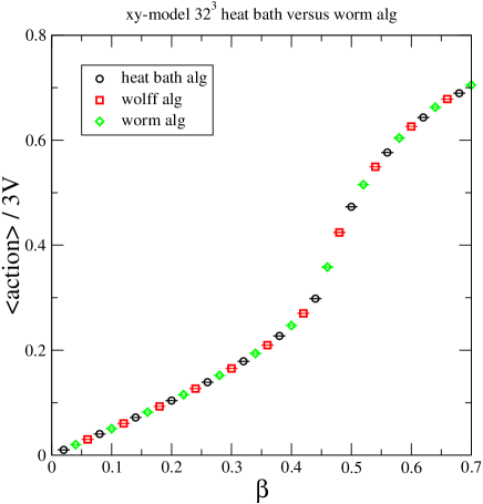
Figure 1: The average action as a function of $\beta$ for the 3d $O(2)$ model using a $32^{3}$ lattice.

Note also that $\chi$ can be viewed as the expectation value for $\sum\cos(\phi)$ where the factor $\cos(\phi_{x_{0}})$ acts as a reference against which the spin orientation is counted. The magnetic susceptibility can be written in a manifestly $O(2)$ invariant form. To this end, we rewrite the expectation value on the right hand side of (14) as

$$\frac{1}{2}\sum_{x}\Bigl{\{}\;\Bigl{\langle}\cos(\phi_{x}-\phi_{x_{0}})\Bigr{\rangle}+\Bigl{\langle}\cos(\phi_{x}+\phi_{x_{0}})\Bigr{\rangle}\;\Bigr{\}}.$$

Using the variable transform (11), we conclude that the latter expectation value vanishes for $j=0$ (at any finite volume). Thus, we can write the magnetic susceptibility as

$$\chi(\beta)\;=\;\frac{1}{2}\sum_{x}\Bigl{\langle}\cos(\phi_{x}-\phi_{x_{0}})\Bigr{\rangle}\;,$$ (15)

which is manifest $O(2)$ invariant. Introducing the spin correlation function, by

$$G(x-y)\;=\;\Bigl{\langle}\vec{n}_{x}\cdot\vec{n}_{y}\,\Bigr{\rangle}\;,$$ (16)

the magnetic susceptibility can be easily related to the integrated spin correlation function:

$$\chi(\beta)\;=\;\frac{1}{2}\,\sum_{x}\,G(x-x_{0})\;.$$ (17)

The latter identity explains the role of $\chi(\beta)$ as an order parameter for the spontaneous breaking of the $O(2)$ symmetry: in the disordered phase, the spin correlation function exponentially decreases over the distance of the correlation length $\xi$, and $\chi(\beta)$ is independent of the system size. If the correlation length near criticality exceeds the system size, we find by means of the sum at the right hand side of (17) that $\chi(\beta)$ diverges with the volume.

III The statistical field theory

III.1 Algorithms and first results

III.1.1 Wolff cluster algorithm

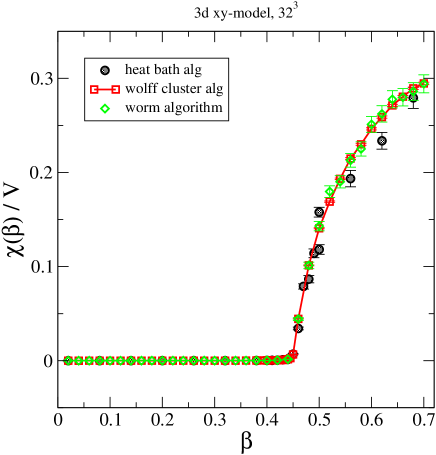
Figure 2: The magnetic susceptibility per volume as a function of $\beta$ for the 3d $O(2)$ model using a $32^{3}$ lattice.

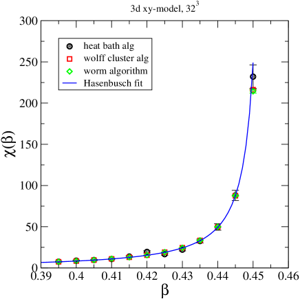
Figure 3: Detail of the magnetic susceptibility as a function of $\beta$ close but smaller than the critical value ($32^{3}$ lattice).

For vanishing chemical potential, i.e., $\mu=0$, and vanishing source $j$, the Wolff cluster algorithm Wolff (1989) offers a very efficient way to simulate the $O(2)$-model. The reason is that the clusters, which are updated in one Wolff step, grasp the physics of the model. This implies that the auto-correlation time depends only weakly on the system size as reflected by a dynamical critical exponent close to zero. The algorithms proceeds as follows:

• Choose a random unit vector $\vec{r}$;

• Activate the link between two neighbouring sites $x$ and $y$ with probability

  $$P(x,y)=1-\exp\left\{\mathrm{min}\left[0,\,-2\,\beta\,(\vec{n_{x}}\cdot\vec{r})\,(\vec{n_{y}}\cdot\vec{r})\,\right]\right\};$$

• Select a random site $x_{0}$ and find the subset $C$ of all spins which are connected to $\phi_{x_{0}}$ by activated links

• Replace

  $$\vec{n}_{x}\to\vec{n}_{x}\,-\,2\,(\vec{n_{x}}\cdot\vec{r})\,\vec{r}\hbox to28.45274pt{\hfill}\forall\;x\in C\;.$$

Observables are best calculated using the so-called improved estimators Hasenbusch (1990); Wolff (1990). In particular, the magnetic susceptibility can be directly related to the cluster properties and as such calculated “on the fly”:

$$\chi(\beta)\;=\;\Bigl{\langle}\frac{1}{V_{c}}\Bigl{(}\sum_{x\in C}\vec{r}\cdot\vec{n}_{x}\Bigr{)}^{2}\,\Bigr{\rangle}\;,$$ (18)

where $C$ denotes a particular Wolff-cluster, and $V_{c}$ is the number of sites belonging to this cluster $C$.

III.1.2 1-shot heat bath algorithm

Heat bath algorithms offer an easy access to expectation values formulated in the terms of the original spin degrees of freedom. We here use the heat bath algorithm to test and benchmark the flux algorithm outlined in the next subsection. For this purpose, we have developed a heat bath algorithm with 100% acceptance rate, which has been inspired by the method from Bazavov and Berg in Bazavov and Berg (2005). In step 1, we choose the spin $\phi_{x}$ for the local update step. If $\langle xy\rangle$ denotes the links joining the sites $x$ and $y$, the action can be written as

$$\Bigl{[} \beta\,\sum_{y\in\langle xy\rangle}\cos(\phi_{y})\,+\,j\Bigr{]}\,\cos(\phi_{x})\;+\;$$

$$\Bigl{[}\beta\,\sum_{y\in\langle xy\rangle}\sin(\phi_{y})\Bigr{]}\,\sin(\phi_{x})\;=\;A\,\cos(\phi_{x}-\psi),$$

where $A$ and $\psi$ depend on $\beta$, $j$ and the neighbouring spins. In step 2, we define

$$f(\phi_{x})\;=\;\int_{-\pi}^{\phi_{x}}\exp\Bigl{\{}A\,\cos(v-\psi)\Bigr{\}}\;dv\;.$$

We then choose a random number $u\in[0,1]$ and solve the equation

$$f(\pi)\;u\;=\;f(\phi_{x})$$

for the new value $\phi_{x}$ for the spin at site $x$. In practice, the integration was performed using the Gauss Legendre method, while the non-linear equation was solved using bisection.

III.1.3 Worm algorithm

For finite values of the chemical potential, i.e., $\mu\not=0$, the action (8) possesses imaginary parts. The theory is hampered by the infamous sign problem and cannot be simulated at reasonably sized lattices using the cluster or the heat bath algorithm. The $O(2)$-model is one of the rare cases where simulations are nevertheless feasible by using the so-called worm algorithm Prokof’ev and Svistunov (2001); Syljuasen and Sandvik (2002); Banerjee and Chandrasekharan (2010); Prokof’ev and Svistunov (2009). The algorithm has been thoroughly discussed in Banerjee and Chandrasekharan (2010). We here briefly review the algorithm for the $O(2)$-model at finite chemical potential before we take it a step further to derive the Kramers-Wannier duality in the next section. Using the identity

$$\mathrm{e}^{\beta\,\cos(\phi)}=\sum_{k=-\infty}^{\infty}I_{k}(\beta)\;\mathrm{e}^{ik\phi}\;,$$ (19)

where $I_{k}=I_{-k}$ is the modified Bessel function of the first kind, the partition function (12) becomes

$$Z[0] = \int{\cal D}\phi_{x}\;\mathrm{e}^{\beta\,S[\phi]}=\int{\cal D}\phi_{x}\;$$ (20)

$$\sum_{\{k_{\ell}\}}\prod_{\ell=\langle xy\rangle}I_{k_{\ell}}(\beta)\;\mathrm{e}^{\mu\delta_{\nu 0}\,k_{\ell}}\;\mathrm{e}^{ik_{\ell}(\phi_{x}-\phi_{y})}$$

$$= \sum_{\{k_{\ell}\}}\prod_{\ell}I_{k_{\ell}}(\beta)\;\mathrm{e}^{\mu\delta_{\nu 0}\,k_{\ell}}\;\prod_{x}\;\delta\left(\sum_{\ell\in x}k_{\ell}\right)\;,$$

where $\nu$ specifies the direction of the link $\ell$. The notation $\ell\in x$ refers to all links which are attached to the site $x$:

$$\sum_{\ell\in x}k_{\ell}\;=\;\sum_{\nu}\Bigl{(}k_{x,\nu}-k_{x-\nu,\nu}\Bigr{)}.$$

If an integer “flux” $k_{\ell}$ is associated with each link $\ell$ of the lattice, the $\delta$-function constraint in (20) implies that the total (directed) flux which enters a site must vanish.

Including the case of a finite chemical potential $\mu$, the worm algorithm has been widely used in Banerjee and Chandrasekharan (2010) to explore properties of the $O(2)$-model. The algorithm works as follows Banerjee and Chandrasekharan (2010):

• Pick a starting point $x$ and set the counter $c=0$

• Choose at random one of the 6 directions (including negative ones); let $y=x+\nu$ be the neighbouring site associated with the chosen direction ($\nu=\pm 1,\pm 2,\pm 3$) and $\ell$ the associated link $\langle xy\rangle=\ell$.

• If a positive direction was selected, with probability $\exp(\mu\delta_{\nu 0})I_{k_{\ell}+1}(\beta)/I_{k_{\ell}}(\beta)$ change $k_{\ell}$ to $k_{\ell}+1$ and move to the neighbouring site $y$. Otherwise stay. In any case, increase $c\to c+1$.

  If a negative direction was selected, with probability $\exp(-\mu\delta_{\nu 0})I_{k_{\ell}-1}(\beta)/I_{k_{\ell}}(\beta)$ change $k_{\ell}$ to $k_{\ell}-1$ and move to the neighbouring site $y$. Otherwise stay. In any case, increase $c\to c+1$.

• Stop if the current position coincides with the starting position, i.e., if $y=x_{s}$.

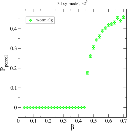
Figure 4: The percolation probability $P_{\mathrm{percol}}$ (25) as a function of $\beta$ ($32^{3}$ lattice).

The average action is easily obtained by

$$A(\beta) = \frac{\partial}{\partial\beta}\,\ln Z\;=\;\sum_{\ell}\,\left\langle\frac{I_{k_{\ell}}^{\prime}(\beta)}{I_{k_{\ell}}(\beta)}\right\rangle\;.$$ (21)

It has been argued in Banerjee and Chandrasekharan (2010) that the magnetic susceptibility is given in terms of the average number of counts $c$:

$$\chi(\beta)\;=\;\frac{1}{2}\,\langle c\rangle\;.$$ (22)

III.1.4 Action average and magnetic susceptibility

High precision simulations of the model have been reported in the literature for zero chemical potential e.g. in Hasenbusch (1990); Campostrini, Massimo and Hasenbusch, Martin and Pelissetto, Andrea and Rossi, Paolo and Vicari, Ettore (2001) and for finite densities in Banerjee and Chandrasekharan (2010). We will benchmark the outcome of our algorithms against these findings before we will move on to study the quantum field theory (QFT) limit at finite densities in the next section. We will employ

• the Wolff algorithm to obtain the correlation length in units of the lattice spacing, which will set the QFT scale,

• the worm algorithm for the simulations at finite densities,

• the heat bath algorithm to crosscheck the numerical results.

To begin with, we have compared all three algorithms by calculating the average action as a function of the coupling $\beta$ using a $32^{3}$ lattice. Our findings are shown in figure 1. We find a nice agreement for all three algorithms for a range of $\beta$ values covering the disordered phase for $\beta<\beta_{c}$, $\beta_{c}=0.45420(2)$ Hasenbusch (1990), as well as the ordered phase $\beta>\beta_{c}$. Our results for the magnetic susceptibility $\chi$ are shown in figures 2 and 3. The transition from the Wigner-Weyl phase to the phase with a spontaneously broken $O(2)$ symmetry is clearly visible in figure 2. As expected the Wolff and the worm algorithm work flawlessly in the broken phase while the results from the heat bath algorithm are plagued by large autocorrelation times. The region of $\beta$ just a bit smaller than $\beta_{c}$ is of particular interest for the QFT limit. Here, all three algorithms perform well (see figure 3). A good agreement with the fit

$$\chi(\beta) = \chi_{0}\,\Bigl{(}1-\frac{\beta}{\beta_{c}}\Bigr{)}^{-\gamma},\hbox to28.45274pt{\hfill}\beta\stackrel{{\scriptstyle<}}{{{}_{\sim}}}\beta_{c}\;,$$ (23)

$$\chi_{0} = 0.5045(1),\;\;\;\beta_{c}=0.45420(2),\;\;\;\gamma=1.324(1)\;,$$

presented in Gottlob and Hasenbusch (1993); Hasenbusch (1990) is observed (note there is a factor of $1/2$ difference in the definition of our magnetic susceptibility and that in Gottlob and Hasenbusch (1993); Hasenbusch (1990)).

III.2 Winding sectors and dual theory

III.2.1 Flux percolation

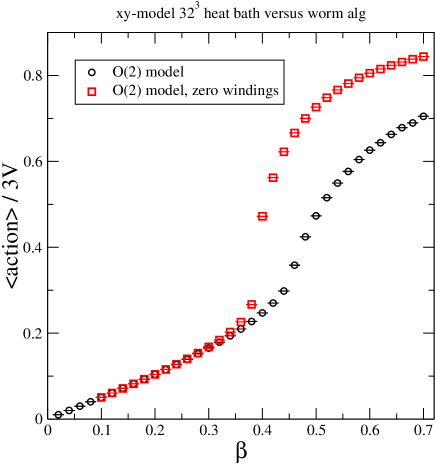
Figure 5: action density for the standard 3d-O(2) model in comparison with model with winding number $n_{w}=0$ only.

By virtue of the periodic boundary conditions, the closed flux lines of the worm algorithm might wind around the torus. Since we currently work with a symmetric lattice of equal size $N$ in all directions, we confine ourselves to the study the winding in time direction. The winding number $n_{\mathrm{w}}$ can be calculated during the construction of a particular flux line. Here, we only need to keep track how often the flux line leaves the torus at the $N_{t}=N$ and $N_{t}=1$, respectively. Every time the flux line leaves the torus at $N_{t}=N$ in positive time direction, we increase $n_{\mathrm{w}}$ by one unit while if the flux line leaves the torus at $N_{t}=1$ negative time direction, we decrease $n_{\mathrm{w}}$ by one unit. One naively might expect that the average winding number is conclusive on the winding of the flux lines. This is, however, not true due to the abundance of small size flux lines which all carry $n_{\mathrm{w}}=0$. The more interesting quantity is the percolation probability $P_{\mathrm{percol}}$: if we choose randomly a particular link of a flux line configuration, how big is the probability that this link is a part of a flux line which at least winds once through the torus? If $L$ denotes the number of links of a particular flux line and if

$$L_{w}\;=\;\left\{\begin{array}[]{ll}L&\hbox{for}\;n_{w}\not=0\\ 0&\hbox{else}\end{array}\right.\;,$$ (24)

the percolation probability is given by

$$P_{\mathrm{percol}}\;=\;\langle L_{w}\rangle\;/\;\langle L\rangle\;.$$ (25)

Figure 4 shows our numerical result as a function of $\beta$. Note that due to the integration of the $\phi_{x}$ in (20) all reference to the global $O(2)$ symmetry has been lost in the flux line representation of the partition function. Here, we find empirically that the flux lines do not percolate in the Wigner-Weyl phase while the flux lines start winding around the torus in the phase with spontaneously broken symmetry. This is intuitively clear by noting that the correlation length diverges for $\beta\to\beta_{c}$. In the flux representation, a finite average cluster size implies a finite correlation length by virtue of (30). Hence, the cluster size necessarily diverges at the critical coupling implying percolation in the finite volume system.

III.2.2 Kramers-Wannier duality

The reformulation of a classical field theory in terms of flux variables has been dubbed the dual formulation in the literature (see e.g. Schmidt et al. (2012)). By its nature, this reformulation is non-local, using the original lattice, and it is therefore quite different from the generic Kramers-Wannier duality, which employs local degrees of freedom related to the dual lattice. Starting from the worm algorithm as formulated in subsection III.1.3, we here derive the dual formulation of the dense $O(2)$ model in the Kramers-Wannier sense. We will find a close relation to the flux formulation: the dual theory turns out to be a gauge theory with the fluxes being the non-local but gauge invariant degrees of freedom of this formulation.

Starting point is the flux formulation (20). Our aim will be to resolve the $\delta$-function constraint on the flux elements $k_{\ell}$ using local variables. Naturally, the emerging dual theory is free of the sign problem at finite chemical potential as the flux line formulation (20) is. To this end, each element of the lattice, i.e., site $x$, link $\ell$, plaquette $p$ and elementary cube $c$, is mapped in the usual way to the dual lattice:

$$x\to\mathbf{c},\hbox to28.45274pt{\hfill}\ell\to\mathbf{p},\hbox to28.45274pt{\hfill}p\to\boldsymbol{\ell},\hbox to28.45274pt{\hfill}c\to\mathbf{x}\;,$$

where the “bold” quantities denote the entities on the dual lattice. Fields depending on the entities are mapped as well, e.g.,

$$k_{\ell}\to k_{\mathbf{p}}\;.$$

The $\delta$-function constraint in (20) then becomes on the dual lattice:

$$\sum_{\ell\in x}k_{\ell}=0\;\;\to\;\;\sum_{\mathbf{p}\in\mathbf{c}}k_{\mathbf{p}}=0\;,$$ (26)

where $\mathbf{p}\in\mathbf{c}$ addresses all plaquettes $\mathbf{p}$ which build up the faces of the cube $\mathbf{c}$. The crucial point is that this constraint can be solved locally for the theory with zero windings. $k_{\mathbf{p}}$ are plaquette variables on the dual lattice, and the latter constraint (26) is reminiscent of the Bianchi identity of a $Z$-gauge theory. Hence, we solve the constraint by introducing the integer valued link field $Z_{\boldsymbol{\ell}}$ of the dual lattice by

$$k_{\mathbf{p}}=\sum_{\boldsymbol{\ell}\in\mathbf{p}}Z_{\boldsymbol{\ell}}$$ (27)

The definition of the links $Z_{\boldsymbol{\ell}}$ which represent the plaquette $k_{\mathbf{p}}$ is not unique. The gauge transformed links,

$$Z^{\Omega}_{\boldsymbol{\ell}=\mathbf{x\mu}}\;=\;\Omega(\mathbf{x})\,+\,Z_{\boldsymbol{\ell}=\mathbf{x\mu}}\,-\,\Omega(\mathbf{x+\mu})\;,$$

where $\Omega(\mathbf{x})$ is integer valued, still give rise to the same plaquette in (27). A $Z$-gauge symmetry arises in the link representation of the dual theory. The partition function (20) of the dual theory can be written as:

$$Z[0] = \sum_{\{Z_{\boldsymbol{\ell}}\}}\;\prod_{\mathbf{p}}I_{k_{\mathbf{p}}}\;\exp\Bigl{\{}\mu\,k_{\mathbf{p^{\prime}}}\Bigr{\}}\;,$$ (28)

where $k_{\mathbf{p^{\prime}}}=k_{\mathbf{p}}$ for spatial plaquettes and $k_{\mathbf{p^{\prime}}}=0$ for time-like plaquettes. The dual formulation sheds light onto the “worms” of the flux line representation. By virtue of (27), this flux is given by the plaquettes of the dual $Z$-gauge theory. On the other hand, the dual plaquette defines the vorticity of the dual theory. Vorticity is conserved by the Bianchi identity, and non-trivial vorticity comes form closed staples of plaquettes. Hence, we find that the closed flux lines, i.e., the “worms”, appear to be the vortices of the dual formulation.

So far, we have established a local equivalence between the standard $O(2)$ model and the $Z$-gauge theory on the dual lattice. For a complete correspondence, we also have to match the boundary conditions of both formulations. This a non-trivial task: let us consider, e.g., periodic boundary conditions for the dual theory. If $\cal A$ is the maximal planar surface in the $xy$-plane and $({\cal A})$ its boundary, we find that the total flux through this plane necessarily vanishes:

$$\prod_{\boldsymbol{\ell}\in({\cal A})}Z_{\boldsymbol{\ell}}\;=\;0\;.$$

On the other hand, the standard formulation of the $O(2)$-model with periodic boundary conditions does not restrict the worm configurations to the sector of zero winding in $z$-direction. Obviously, we have to give up periodic boundary conditions for the $Z$-gauge theory if we want correspondence. If $n_{w}$ is the worm winding number, the corresponding $Z$-gauge theory simulating this sector features non-trivial boundary conditions such as

$$Z_{2}(x=1,1,1) = Z_{2}(x=N_{x},1,1)+n_{w},$$

(periodic else),

where the subscript “$2$” indicates the y-direction of the link. The issue, however, is that it is a priori unknown with which weight these winding sectors must contribute in order to correspond to the standard $O(2)$ model with periodic boundary conditions. We expect, however, that the non-trivial winding sectors are not important in the disordered phase. In this case, we would expect a correspondence between the standard and the dual formulation both with periodic boundary conditions.

We have verified this by a direct simulation. The action density calculated with the $Z$-gauge theory with periodic boundary conditions (i.e., zero winding number $n_{w}=0$) is contrasted to the result from the $O(2)$ model with periodic boundary conditions in figure 5. As expected, both action densities agree in the strong coupling phase for $\beta\ll\beta_{c}$. For $\beta\stackrel{{\scriptstyle<}}{{{}_{\sim}}}\beta_{c}$, the correlation length is sufficiently large to observe a sizable dependence on the boundary conditions. Large differences are observed in the broken phase when windings have a role to play.

We find that the 3d $O(2)$ (or $xy$) model is dual to a theory of vortices. This might explain part of its phenomenological success for solid state systems the thermodynamics of which are influenced by vortex dynamics (see e.g. Kamal et al. (1994)).

IV Quantum field theory - Wigner-Weyl phase

IV.1 Finite temperatures

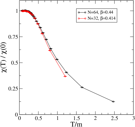
Figure 6: Magnetic susceptibility $\chi$ in the QFT limit of the 3d $O(2)$ model as a function of the temperature $T$ in units of the mass gap.

Here, we study the emerging quantum field theory in the critical limit of the $O(2)$ statistical field theory. We will consider finite temperatures, but we will confine ourselves to zero density.

If we approach the critical coupling $\beta_{c}$ from below, i.e., $\beta\stackrel{{\scriptstyle<}}{{{}_{\to}}}\beta_{c}$, the $O(2)$ theory remains in the Wigner-Weyl phase, while the correlation length $\xi(\beta)$ in units of the lattice spacing $a$ diverges. For $\beta$ close to the critical coupling, one finds a scaling relation of the type Gottlob and Hasenbusch (1993):

$$\xi(\beta)\;=\;\xi_{0}\,\cdot\,\left(1-\frac{\beta}{\beta_{c}}\right)^{-\nu}\;.$$ (29)

The correlation length is best calculated using an improved estimator and the Wolff algorithm. In fact, it was shown that the spin correlation function (16) can be estimated by Hasenbusch (1990); Wolff (1990):

$$G(x-y)\;=\;2\,\Bigl{\langle}\frac{N^{3}}{V_{c}}\,(\vec{r}\cdot\vec{n}_{x})\,(\vec{r}\cdot\vec{n}_{y})\,\theta(C,x)\,\theta(C,y)\,\Bigr{\rangle}\;,$$ (30)

where

$$\theta(C,x)\;=\;\left\{\begin{array}[]{ll}1&\hbox{for}\;x\in C\\ 0&\hbox{else.}\end{array}\right.$$

The scaling parameters have been obtained to good accuracy by fitting the scaling relation (29) to Monte-Carlo data. Reference Gottlob and Hasenbusch (1993) reports

$$\beta_{c} = 0.454157(14),\;\;\;\nu\;=\;0.6711(16),$$ (31)

$$\xi_{0} = 0.4866(26)\;.$$

from an analysis of high precision data. For large correlation length, the theory becomes independent from the underlying lattice structure and can be effectively described by a quantum field theory (QFT). The QFT limit is attained by defining a fundamental length scale which plays the role of the only free parameter of this theory. Here, we choose the so-called mass gap $m$ of the theory which is provided by the inverse correlation length. The scaling relation (29) then implies a dependence of the lattice spacing $a$ on the “bare coupling” $\beta$:

$$m\,a(\beta)=\xi^{-1}(\beta)\;.$$ (32)

The bare coupling $\beta$ is tuned towards the critical coupling. This implements the QFT limit by sending the lattice spacing (in physical units) to zero. The bare coupling $\beta$ is no longer a free parameter of the theory, but its role has been taken over by the dimensionful parameter $m$ (dimensional transmutation). In following, we will use (32) to eliminate the lattice regulator $a(\beta)$ in favour of the physical mass parameter $m$ and will assume that (29) is a good approximation for the true correlation length $\xi(\beta)$ for the range of $\beta$ values used throughout this paper. This assumption is checked by calculating observables at different renormalisation points $\beta$ and in physical units. Any violations of the scaling relation would then be detected by a non-universal behaviour. For the choice of $\beta$ values below, we found good universal scaling for the observables under discussions.

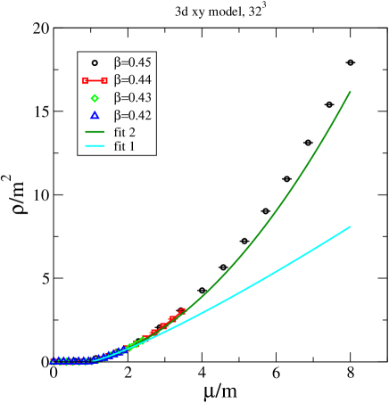
Figure 7: The charge density $\rho$ as function of the chemical potential in units of the mass gap $m$ in the QFT limit ($32^{3}$ lattice).

QFT observables are constructed from the “bare” observables by scaling the quantity of interest in units of the mass gap $m$ (to the power of its canonical dimension) and by taking into account the wave function renormalisation. Because of its relation to the correlation function, the canonical dimension of the magnetic susceptibility is two, and we write:

$$Z_{\chi}(\beta)\,\chi(\beta)\;=\;\chi_{\mathrm{qft}}a^{2}\;,$$ (33)

where $Z_{\chi}$ is the wave function (or better composite operator) renormalisation constant. With the help of (23), (29) and (32), we find:

$$\chi_{\mathrm{qft}}/m^{2}=Z_{\chi}(\beta)\,\frac{\chi(\beta)}{\xi^{2}(\beta)}=Z_{\chi}(\beta)\,\frac{\chi_{0}}{\xi_{0}^{2}}\,\Bigl{(}1-\frac{\beta}{\beta_{c}}\Bigr{)}^{2\nu-\gamma}\;.$$ (34)

In a “minimal subtraction scheme”, we would choose

$$Z_{\chi}(\beta)\;=\;\Bigl{(}1-\frac{\beta}{\beta_{c}}\Bigr{)}^{-\,d_{\chi}}\;,$$ (35)

where the anomalous dimension for this operator $d_{\chi}$ turns out to be quite small:

$$d_{\chi}\;=\;\gamma-2\nu\;\approx\;-0.018(2)\;.$$ (36)

Needless to say that the actual value of the renormalised quantity $\chi_{\mathrm{qft}}$ must be fixed by a renormalisation condition.

Finite temperatures, i.e., $T\not=0$, are implemented by reducing the extent of the lattice in the time direction:

$$T\;=\;\frac{1}{N_{t}\,a(\beta)}\hbox to28.45274pt{\hfill}T/m\;=\;\xi(\beta)/N_{t}\;,$$ (37)

where $N_{t}$ is the number of lattice points in time direction. Once the observable has been renormalised achieving vacuum values which enjoy a physical interpretation in the continuum limit $a\to 0$, we can start to make predictions at e.g. finite temperatures. Here, we study the temperature dependence of the magnetic susceptibility. To this aim, we primarily carried out calculations at $\beta=0.44$ using a $64^{2}\times N_{t}$ lattice. For a study of the lattice spacing (in-)dependence, we also did simulations utilising a $32^{2}\times N_{t}$ lattice and $\beta=0.414$. Note that both simulations implement roughly the same spatial volume since

$$a(\beta=0.414)\approx 2\,a(\beta=0.44)\;.$$

Our findings are summarised in figure 6. The overall agreement between the two curves is satisfactory bearing in mind that the last points at large $T$ correspond to $N_{t}=2$ for which we might expect quite some rotational symmetry breaking effects. We observe the magnetic susceptibility stays roughly constant for $T\stackrel{{\scriptstyle<}}{{{}_{\sim}}}0.4\,m$ while for $T\approx m$ it has fallen approximately to half its vacuum value.

IV.2 Cold, but dense matter

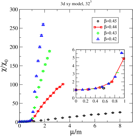
Figure 8: Magnetic susceptibility $\chi$ in the QFT limit of the 3d $O(2)$ model as a function of the chemical potential $\mu$ in units of the mass gap.

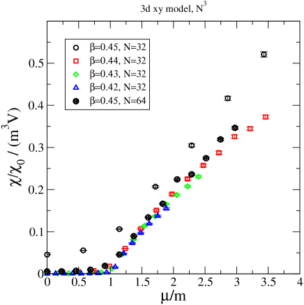
Figure 9: Magnetic susceptibility $\chi$ per total volume as a function of the chemical potential $\mu$ ($N^{3}$ lattice).

Let us now study finite densities by turning on the chemical potential. The physical chemical potential $\mu_{\mathrm{phys}}$ is related to the bare chemical potential $\mu$, the parameter e.g. featuring in (20), by

$$\mu=\mu_{\mathrm{phys}}\,a\;\;\;\Rightarrow\;\;\;\mu_{\mathrm{phys}}/m\;=\;\xi(\beta)\,\mu\;.$$ (38)

We will do so at zero temperatures, which are adopted by performing simulations using a symmetric lattice, $N=N_{t}$. Again, we study the QFT limit of the $O(2)$ theory, but now for non-zero values of the chemical potential.

The first observable which we will study is the matter density. The matter density is easily accessible using the worm algorithm (see (20)):

$$\rho = \frac{T}{V_{2}}\frac{\partial\ln Z}{\partial\mu_{\mathrm{phys}}}\;=\;\frac{1}{V_{2}N_{t}}\frac{\partial\ln Z}{\partial\mu}$$ (39)

$$= \frac{1}{V_{2}}\,\Bigl{\langle}\sum_{x\in\hbox{time slice}}k_{\ell}\Bigr{\rangle}\;,\;\;\;\ell=\langle x,0\rangle,$$

where $V_{2}=N^{2}a^{2}$ is the “spatial” volume and the summation extends over all sites $x$ which are part of a given time slice (see also Banerjee and Chandrasekharan (2010)). Due to current conservation, any choice for the time slice gives the same answer. In physical units, we find

$$\rho/m^{2}\;=\;\frac{\xi^{2}(\beta)}{N^{2}}\,\Bigl{\langle}\sum_{x\in\hbox{time slice}}k_{\ell}\Bigr{\rangle}\;\;\;\ell=\langle x,0\rangle.$$ (40)

Since the charge is conserved, there is no wave function renormalisation of the density. This is confirmed by a direct calculation (see figure 7) using several $\beta$ values ranging from $0.42$ to $0.45$ implying that the corresponding lattice spacing $a$ changes by a factor of approximately $4.2$. Yet, the density in physical units nicely falls on top of a uniform curve. Most importantly, we observe that the density vanishes for chemical potentials smaller than the mass gap, i.e., $\mu<m$. With other words, the onset chemical potential agrees with the mass gap, and the simulation is free of a Silver-Blaze problem Cohen (2003). Secondly, the density smoothly starts to rise with the chemical potential at the onset value. This is markedly different from the case of a free Bose gas for which we would observe that the density diverges logarithmically when approached from above. This would indicate the well known phenomenon of Bose-Einstein condensation. However, our data are more compatible with a quadratic rise of the density with the chemical potential which is reminiscent of a free 2d Fermi gas at low temperatures:

$$\rho_{\mathrm{Fermi}}\propto(\mu-m)^{2}\;.$$

Although the standard $O(2)$ model is formulated in terms of bosonic degrees of freedom, it is not ruled out that the model near the onset transition is well described by an effective fermion theory. To trace this out further, we have fitted the numerical data in figure 7 to a simple scaling law:

$$\rho/m^{2}\;=\;a_{0}\,(\mu/m-1)^{a_{1}}\;.$$ (41)

We find, however, that the data are not well represented by this ansatz. Performing independent fits to each set for a given $\beta$, the results are collated in the first two rows of table 1:

	$\beta=0.42$	$\beta=0.43$	$\beta=0.44$	$\beta=0.45$
$a_{0}$	$0.77(1)$	$0.82(1)$	$0.827(5)$	$0.70(2)$
$a_{1}$	$1.2(1)$	$1.27(2)$	$1.42(2)$	$1.66(2)$
$b_{0}$	$0.54(2)$	$0.55(2)$	$0.55(2)$	$0.58(1)$
$b_{1}$	$0.25(3)$	$0.26(2)$	$0.27(1)$	$0.281(6)$

Table 1: Fitting the density to the power law ansatz (41) and to (42).

We point out that the data are quite well fitted by the ansatz

$$\rho/m^{2}\;=\;b_{0}\,\mu/m\;+\;b_{1}\,(\mu/m)^{2}\;.$$ (42)

The coefficients $b_{0}$, $b_{1}$ are also listed in table 1. Figure 7 shows the curves from the fit according to (41), called fit 1, and according to (42) called fit 2. The fitting curves have been generated using the fit parameters obtained for $\beta=0.42$.

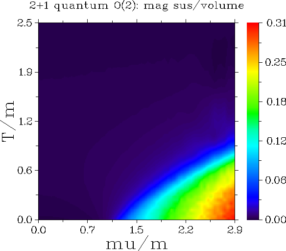
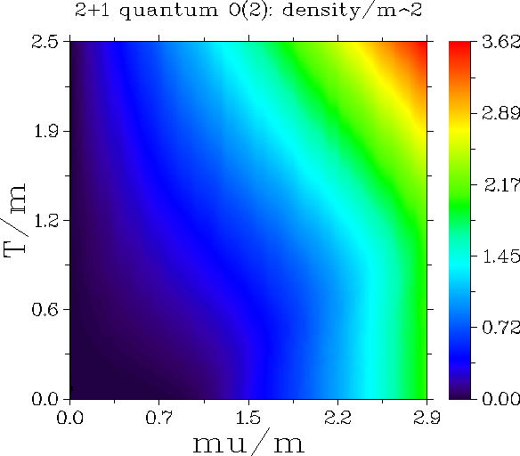
Figure 10: Phase diagram: Magnetic susceptibility $\chi$ per total volume (left) and density (right).

It is interesting to note that a free Fermi gas at small, but non-zero temperature would suggest the $\mu$-dependence shown in (42). In this case, the fitting coefficient $b_{0}$ should be proportional to the temperature. In order to explore the potential correspondence between the $O(2)$ quantum model and a Fermi gas, further simulations for different lattice sizes and aspect ratios are necessary. This is left to future studies. We also point out that in the case of a free gas of hardsphere bosons Bernardet et al. (2002) one expects a linear rise of the density with the chemical potential $\mu\stackrel{{\scriptstyle>}}{{{}_{\sim}}}\mu_{c}$. Note, however, that the coefficient $b_{1}$ should be negative in the latter case.

Let us finally explore the magnetic susceptibility $\chi$ below and above the onset value of the chemical potential. Figure 8 shows $\chi$ normalised to its zero temperature value $\chi_{0}$ in order to remove the renormalisation constant. The inlay of this figure shows that $\chi/\chi_{0}$ is indeed independent of the renormalisation point specified by $\beta$. Although the density remains zero for $\mu<m$, the chemical potential impacts on the properties of the theory as indicated by the increase of $\chi/\chi_{0}$ with $\mu$. For $\mu>m$, the data for $\chi/\chi_{0}$ largely depend on the value $\beta$. Note that the simulations (except for $\beta=0.45$) are carried out for a fixed number of lattice points. Here, a change of $\beta$ also implies a change of the lattice volume. This is indeed the cause for the apparent scaling violations: Figure 9 shows the magnetic susceptibility per volume, i.e., $\chi/\chi_{0}/(m^{3}V)$. The volume $V$ is the physical volume and the mass gap is introduced to render this factor dimensionless. The factor $\chi_{0}$ is again necessary to remove the renormalisation constant. We observe good scaling for the magnetic susceptibility in units of the (physical) volume for a wide range of $\beta$ values. An exemption is the result for $\beta=0.45$. For this $\beta$, the correlation length equals roughly a third of the system size and finite volume effects come into play. At $\beta=0.45$, we also calculated $\chi/\chi_{0}/(m^{3}V)$ for a $N^{3}=64^{3}$ lattice. A good agreement with the results from smaller $\beta$ and for a $N^{3}=32^{3}$ lattice is recovered. We interpret the physics behind these findings as follows: For $\mu>m$, matter starts populating the ground state. This alters the interaction between the spins such that the U(1) global symmetry of the model breaks spontaneously leading to a superfluid phase.

We are finally in the position to calculate the phase diagram of the $2+1$ dimensional quantum $O(2)$-theory in the $\mu/m$ and $T/m$ plane. We have carried simulations with $\beta=0.44$ using a lattice size of $64\times N_{t}$, where $N_{t}=2\ldots 32$. We performed simulations for $\mu a=0.01\ldots 0.6$ in steps of $0.01$. Naturally, the temperature steps from (37) are not equally spaced. We used a cubic spline interpolation to generate a regularly spaced $60\times 60$ data set before plotting.

To detect the superfluid phase in the phase diagram, we plotted the renormalised magnetic susceptibility in units of the physical volume, i.e., $\chi/\chi_{0}/(m^{3}V)$ where $V$ is the (physical) volume of the 3-torus, i.e., $V=L^{2}/T$. The result is shown in figure 10, left panel. As expected, we find the superfluid phase in the cold, but dense region. Increasing temperature at a fixed chemical potential $\mu>m$, rapidly dissolves the superfluid phase. Also shown is the density in the $\mu$-$T$-plane. At low temperatures, we observe the onset at $\mu\geq m$. For $\mu\approx m$, we observe an increase of the density with temperature, which is due to thermal excitations with more particles overcoming the mass gap than anti-particles.

V Conclusions

Using existing simulations techniques such as the Wolff cluster algorithm and the worm algorithm, we have thoroughly analysed the 3d $O(2)$ model in the continuum limit $\beta\to\beta_{c}$. In this limit, the model represents the quantum $O(2)$ model in $2+1$ dimensions. The mass gap $m$ takes over the role of the free (scale) parameter, while the lattice spacing $a$ is fine-tuned by the $\beta$ dependent correlation length, $ma(\beta)=1/\xi(\beta)$.

We have analysed the zero density limit by calculating the (renormalised) magnetic susceptibility as a function of the temperature. As usual, the temperature depends on the extent $N_{t}$ of the torus in time direction, i.e., $T/m=\xi(\beta)/N_{t}$. We find good scaling over more than a factor of $4$ in the lattice spacing. The magnetic susceptibility is rather independent of the temperature for $T<m/2$ while a rather steep descent is observed for $T\stackrel{{\scriptstyle>}}{{{}_{\sim}}}m$.

Charge is defined by means of the Noether current of the global $U(1)$ symmetry of the theory, and finite densities are introduced using the chemical potential $\mu$. In a first step, we analysed the $\mu$ dependence of the (renormalised) magnetic susceptibility and the density at “zero” temperature (isotropic lattice). Simulations are carried out using the worm algorithm. The onset chemical potential $\mu_{c}$ is found to agree with the mass gap $m$ of the theory. At $\mu\stackrel{{\scriptstyle>}}{{{}_{\sim}}}\mu_{c}$, the density smoothly rises with increasing $\mu$ ruling out Bose-Einstein condensation. In fact, the $\mu$ dependence of the density is more in line with a free Fermi gas (at small temperatures). More investigations are needed to understand the theory close to onset in terms of an effective theory. This is left to future work.

For $\mu\geq\mu_{c}$, the magnetic susceptibility scales with the volume and signals the spontaneous breakdown of the $U(1)$ symmetry and therefore superfluidity. We finally present the results for the full $\mu$-$T$ phase diagram. In the cold, but dense regime we find a superfluid phase, which is rapidly resolved by increasing the temperature.