Noise reduction by coupling of stochastic processes and canalization in biology

today

Randomness is an unavoidable feature of the intracellular environment due to chemical reactants being present in low copy number. That phenomenon, predicted by Delbrück long ago [1], has been detected in both prokaryotic [2, 3] and eukaryotic [4] cells after the development of the fluorescence techniques. On the other hand, developing organisms, e.g. D. melanogaster, exhibit strikingly precise spatio-temporal patterns of protein/mRNA concentrations [5, 6, 7, 8]. Those two characteristics of living organisms are in apparent contradiction: the precise patterns of protein concentrations are the result of multiple mutually interacting random chemical reactions. The main question is to establish biochemical mechanisms for coupling random reactions so that canalization, or fluctuations reduction instead of amplification, takes place. Here we explore a model for coupling two stochastic processes where the noise of the combined process can be smaller than that of the isolated ones. Such a canalization occurs if, and only if, there is negative covariance between the random variables of the model. Our results are obtained in the framework of a master equation for a negatively self-regulated – or externally regulated – binary gene and show that the precise control due to negative self regulation [9] is because it may generate negative covariance. Our results suggest that negative covariance, in the coupling of random chemical reactions, is a theoretical mechanism underlying the precision of developmental processes.

We approach the stochastic model for a binary gene operating under negative self-regulation or external regulation [10, 11]. Analytic solutions for the steady state [12, 13] and the dynamic [14, 15] regimes, as well as the symmetries [16, 17] underlying solubility have already been presented. This system has the transcription and translation treated as combined processes. The state of the system is defined by two stochastic variables, the gene state (activate or repressed) and the protein number in the cytoplasm. The gene state is defined effectively in terms of its promoter site as on/off under the action of an external agent, e.g. a protein codified by another gene, or by self-interaction.

We consider a stochastic formulation for the dynamics of the probability of finding the gene in an active (or repressed) state, indicated by $\alpha_{n}$ (or $\beta_{n}$) when $n$ proteins are found in the cytoplasm. The protein synthesis rates are given by $k$ or $\chi k$ ($0\leq\chi<1$) when the gene is, respectively, turned “on” or “off”. The degradation rate of the proteins is given by $\rho$. The “off-on” switching rate is denoted by $f$ while $h_{1}$ and $h_{2}$ indicate the opposite transition rates. The master equation is:

$$\dfrac{d\alpha_{n}}{dt} = k(\alpha_{n-1}-\alpha_{n})+\rho[(n+1)\alpha_{n+1}-n\alpha_{n}]$$ (1)

$$- ({h}_{1}n+{h}_{2})\alpha_{n}+{f}\beta_{n},$$

$$\dfrac{d\beta_{n}}{dt} = \chi k(\beta_{n-1}-\beta_{n})+\rho[(n+1)\beta_{n+1}-n\beta_{n}]$$ (2)

$$+ ({h}_{1}n+{h}_{2})\alpha_{n}-{f}\beta_{n}.$$

The existence of an “on-off” transition dependent on $n$ indicates a negative self-regulating gene ($h_{2}=0$). For an externally regulated gene, one assumes $h_{1}$ to be zero. The proportionality to $n$ is effective and has no relationship with the actual biochemical mechanisms of protein binding/unbinding to DNA regulatory regions, that might involve a plethora of chemical reactions.

Eqs. (1) and (2) might be considered as the coupling of two different Poissonian processes, each of them related to one of the gene states. The processes are coupled in terms of a second stochastic variable, the gene state. To each gene state, we associate the quantities $N_{1}=k/\rho$ and $N_{2}=\chi k/\rho$, that are the stationary averages of the isolated Poisson processes. Therefore, the biologically measurable quantities are the protein number in the cytoplasm $n$ and the protein synthesis rates $\{N_{1},N_{2}\}$ and proceed to evaluating the noise on $n$.

For that purpose, we start defining the moments of the random variables $(n,N)$ in terms of $\alpha_{n}$ and $\beta_{n}$ as:

$$\langle n^{p}N^{q}\rangle=\displaystyle\sum_{n=0}^{+\infty}(\alpha_{n}N_{1}^{q}+\beta_{n}N_{2}^{q})n^{p}.$$ (3)

The marginal probabilities of finding $n$ proteins inside the cell are given by $\phi_{n}=\alpha_{n}+\beta_{n}$, and the protein synthesis rate has a probability $p_{1}=\sum_{n=0}^{\infty}\alpha_{n}$ (or $p_{2}=\sum_{n=0}^{\infty}\beta_{n}$) to be $N_{1}$ (or $N_{2}$).

As we have two random variables, it is convenient to use the covariance between $n$ and $N$ – indicated by $\xi_{i,n}$ – for the analysis of the variance on the number of gene products, namely

$$\xi_{n,i}=\langle nN\rangle-\langle n\rangle\langle N\rangle.$$ (4)

The noise on the protein number of the composed system of the Eqs. (1) and (2) is computed in terms of the Fano factor, that is defined as the ratio between the variance and the mean of $n$,

$$\mathcal{F}=\frac{\langle n^{2}\rangle-\langle n\rangle^{2}}{\langle n\rangle}.$$ (5)

As a Poisson (or Fano) distribution has a Fano factor equals to unity, the Fano factor is used to determine how different from the Poissonian a probability distribution is. When $\mathcal{F}>1$ the distribution is spreader and named super-Poisson (or super-Fano) while it is named sub-Poisson (or sub-Fano) when $\mathcal{F}<1$. As it is shown at the supplementary material, at the stationary limit, the Fano factor can be reduced to

$$\mathcal{F}=1+\frac{\xi_{n,i}}{\langle n\rangle},$$ (6)

which value depends on the signal of the covariance between the two stochastic variables of the model. It is worth to mention that this relation for the Fano factor holds for a gene operating in two, three and so on, states of synthesis.

Eq. (6) shows the possibility of occurrence of sub, super or Poissonian distributions when we deal with the probability distributions generated by the Eqs. (1) and (2), depending on the value of $\xi_{n,i}$. As we shall show below, for an external regulating gene, the covariance, $\xi_{n,i}^{e}$ satisfies

$$\xi_{n,i}^{e}\geq 0.$$ (7)

The negatively self-regulating gene might have the covariance, $\xi_{n,i}^{s}$, to be

$$\xi_{n,i}^{s}\geq 0,\ \ {\rm or}\ \ \xi_{n,i}^{s}<0.$$ (8)

Thus, while an externally regulated gene operates only on the super-Poisson and Poisson regimes, the negative self-regulated gene operates on both regimes plus the sub-Poissonian.

A closed form for Eqs. (7) and (8), for the binary gene, is written with the help of the exact solutions of the Eqs. (1) and (2) [12, 13]. Before writing the closed forms for the covariance for the externally regulated or self-interacting gene, we redefine the model’s parameters as:

$$z_{0} = \frac{\rho}{\rho+h_{1}},\ \ N_{1}=\frac{k}{\rho},\ \ a=\frac{f}{\rho},$$

$$b = \frac{f+h_{2}}{\rho}z_{0}\,+\,N_{1}z_{0}(1-z_{0}).$$ (9)

Particularly, one takes $z_{0}=1$ (or $h_{1}=0$) and it results

$$b=\frac{f+h_{2}}{\rho},$$ (10)

for the externally regulated gene and $0\leq a\leq b$ when one compares the Eqs. (Noise reduction by coupling of stochastic processes and canalization in biology) and (10). The negative self-regulating gene has $h_{2}=0$ and

$$b=[a+N_{1}(1-z_{0})]z_{0}.$$ (11)

In the set of parameters $\{a,b,z_{0}\}$ one takes $N_{1}=\dfrac{b-az_{0}}{z_{0}(1-z_{0})}$ and, due to positivity of $N_{1}$, we see that, for a fixed $b$, $a$ lies in the interval $[0,b/z_{0}]$. The choice for a fixed $b$ is because it is the invariant characterizing the Lie symmetry of the binary model [16, 17]. Now we present explicit forms for the covariances, which demonstration is given at the supplementary material.

The covariance of the extenally regulated gene ($z_{0}=1$) is given by

$$\xi^{e}_{n,i}=\frac{N_{1}^{2}}{b+1}\frac{a}{b}\frac{b-a}{b}\geq 0,$$ (12)

since $a\leq b$.

For negatively self-regulating gene ($h_{2}=0$) the covariance has a more complicated form, given in terms of the protein mean number $\langle n\rangle=CN_{1}(az_{0}/b){\rm M}(a+1,b+1,N_{1}z_{0}(1-z_{0}))$. Namely it is given as:

$$\xi^{s}_{n,i}=az_{0}\frac{N_{1}-\langle n\rangle}{1-z_{0}}-\langle n\rangle^{2},$$ (13)

where we used the Eq. (Noise reduction by coupling of stochastic processes and canalization in biology). The reader should keep in mind that the average protein number is given as a function of the parameters $(a,b,z_{0})$ and $\langle n\rangle$ is used for shortness.

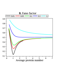
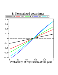
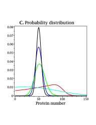
Figure 1: A. Fano factor versus the average protein number. Here we fixed $a=500$ with different colors standing for fixed values of $b$ as indicated on the legend. The Fano factor for the binary gene has 0.5 as an assymptotic limit, when the protein numbers tend to their maximum value, when $z_{0}\rightarrow 0$. This limit corresponds to the condition of protein degradation very slow. The behaviour of $\mathcal{F}$ is dependent on the value of $b$ when $z_{0}\rightarrow b/a$. It has a simple decay to 0.5 for $b>0.1$ while it presents a pronounced minimum at $\langle n\rangle=1$ for the values of $b\leq 0.1$. Surprisingly, the lowest value for the Fano factor occurs on the limit of low molecules number. B. Normalized covariance versus the probability to the gene to be active. At that graphic we have plotted the Eq. (14) versus $p_{2}$. We have fixed $z_{0}=0.45$ and, for each value of $b$, we varied $a$ from zero to $b/z_{0}$. The correlation is positive for $a<b$ and negative for $a>b$. For $a=b$ we have $p_{2}=1-z_{0}$ and the correlation is null. C. Probability distribution of the protein number for the negatively self-regulating gene ($\phi_{n}=C\frac{(a)_{n}}{(b)_{n}}\frac{(N_{1}z_{0})^{n}}{n!}{\rm M}(a+n,b+n,-Nz_{0}^{2})$). The coupling between the “on” and “off” states sharpens the probability distribution as shown by the increase of the parameters $a$ and $z_{0}$. The constants ($a$, $b$, $z_{0}$) for the lines in black, blue, green, cyan and red, are, respectively, ($5\times 10^{3}$, 1., $10^{-4}$), (50., 50., 0.5), (14., 70., 0.5), (1., 15., 0.95), (1., 2., 0.99).

Fig. (1) A shows the Fano factor versus the average protein number, for a fixed value of $a$, for the negative self-interacting gene. Each line corresponds to a fixed value of $b$ and variation of $z_{0}$. As it have been demonstrated earlier [16], the sub-Fano regimes occur only when $a>b$. Since we are exclusively interested on the sub-Fano regime we have investigated only the condition $a>b$, that corresponds to the negative covariance regime. Unexpectedly, there is a minimum value for the Fano factor for the mean protein number equals to one. The Fano factor, for the higher values of the average protein number, is smaller than the Fano factor for the Poisson process by a factor 2.

Fig. (1) B shows the covariance, as calculated from the ratio between the covariance by the variance on $n$ and the variance on $N$, namely

$$\xi^{s}_{i,n}/\sigma/\sqrt{N_{1}^{2}p_{1}p_{2}},$$ (14)

versus the probability for the gene to be active, $p_{1}$. The covariance is positive for $p_{1}<z_{0}$ (or $a<b$), when the gene has a high probability to stay repressed. The covariance is zero for $p_{1}=z_{0}$ (or $a=b$) and $\phi_{n}$ shall be a Poissonian distribution. For the condition when $p_{1}>z_{0}$ (or $a>b$), the covariance is negative and one obtains a sub-Fano regime, with located probability distributions.

Fig. (1) C shows the effect of increasing the intensity of coupling of the two gene states onto the probability distribution $\phi_{n}$ of finding $n$ proteins inside the cell in the negatively self-regulating gene. The spreader distributions, as shown by the colors cyan and red, correspond to the condition of $a$ and $z_{0}$, respectively, close to 0 and 1, that is the limit of low values for the switching rate (or coupling) constants $f$ and $h_{1}$ at the Eqs. (1) and (2). For intermediary values of the coupling constants, the distribution is still super-Poisson and gets thinner, as shown by the green colored line. A Poisson distribution is represented by the blue line. The limit when $a>b$ and $z_{0}\sim 0$, for strong coupling, the probability gets highly located, as indicated by the black line.

In the case of a sub-Poissonian process of protein synthesis, the Fano factor is smaller than that of the uncoupled Poissonian processes. Hence, the negative covariance induces canalization when two stochastic processes are coupled. We suggest this as the theoretical mechanism underlying the higher precision of the negative self-regulating gene [9]: the possibility of regimes where negative covariance between protein number and gene synthesis rates (or, equivalently, gene states) exists.

Finally, the variance, $\sigma^{2}$, on the number of products of a gene operating in multiple modes of synthesis follows directly from the expression for the Fano factor as

$$\sigma^{2}=\langle n\rangle+\xi_{n,i}.$$ (15)

It is clear from this equation that the variance for the negatively self-regulating binary gene is smaller than that of Poissonian distribution, for a fixed average protein number, when the covariance between the protein number and the gene state is negative. In other words, the probability distribution on $n$ shall be highly located around $\langle n\rangle$.

The existence of a negative covariance on a negatively self-regulating gene is intuitively predicted from the analyzis of the Eqs. (1) and (2). The coupling between these two equations is given as a function of $n$. That is interpreted as follows, the higher the number of proteins in the cytoplasm of the cell, the higher the probability for the gene to switch to the repressed state and, consequently, to have a lower value for the protein synthesis rate, i.e., an increase in $n$ might decrease $N$. Despite not easy to demonstrate, it is tempting to conjecture the existence of negative covariance regimes in negatively self-regulating genes operating in more than two modes of expressio.

Biologically, the cell processes requiring higher precision would have a biochemical machinery that implement the negative covariance. Furthermore, one would expect the gene to switch multiple times during a time interval without a significant change of the protein number. Under these two assumptions it is expectable that the variance on the protein number to be small.

In summary, in this manuscript we have shown that the higher precision on the number of gene products by the stochastic gene under negative self-regulation is due to the negative covariance between two random variables: protein number and protein synthesis rate. Our results suggest this as a general mechanism underlying the variance reduction (or canalization) in the cell environment. Further research should enlighten the biochemical implementation of negative covariance in networks or cascades of biochemical reactions. Experimental verification of our results would employ detection of both gene activation and protein numbers and analysis of their covariance.

References

- [1] M. Delbrück. Statistical fluctuations in autocatalytic reactions. J. Chem. Phys., 8:120–124, 1940.
- [2] M. B. Elowitz, A. J. Levine, E. D. Siggia, and P. S. Swain. Stochastic gene expression in a single cell. Science, 297:1183–1186, 2002.
- [3] L. Cai, N. Friedman, and X. S. Xie. Stochastic protein expression in individual cells at the single molecule level. Nature, 440:358–62, 2006.
- [4] W. J. Blake, M. Kaern, C. R. Cantor, and J. J. Collins. Noise in eukaryotic gene expression. Nature, 422:633–637, 2003.
- [5] T. Gregor, D. W. Tank, E. F. Wieschaus, and W. Bialek. Probing the limits to positional information. Cell, 130:153–164, 2007.
- [6] Manu, S. Surkova, A. V. Spirov andV. Gursky, H. Janssens, A. Kim, O. Radulescu, C. E. Vanario-Alonso, D. H. Sharp, M. Samsonova, and J. Reinitz. Canalization of gene expression in the Drosophila blastoderm by gap gene crossregulation. doi:10.371/journal.pbio.1000049, 2009.
- [7] Manu, S. Surkova, A. V. Spirov andV. Gursky, H. Janssens, A. Kim, O. Radulescu, C. E. Vanario-Alonso, D. H. Sharp, M. Samsonova, and J. Reinitz. Canalization of gene expression and domain shifts in the Drosophila blastoderm by dynamical attractors. PLoS Computational Biology, 5:e1000303, 2008. doi:10.1371/journal.pcbi.1000303.
- [8] Alistair N. Boettiger and Michael Levine. Synchronous and stochastic patterns of gene activation in the drosophila embryo. Science, 325:471–3, 2009.
- [9] A. Becskei and L. Serrano. Engineering stability in gene networks by autoregulation. Nature, 405(6786):590–3, 2000.
- [10] M. Sasai and P. G. Wolynes. Stochastic gene expression as a many-body problem. Proc Natl Acad Sci U S A, 100(5):2374–9, 2003.
- [11] J. Peccoud and B. Ycart. Markovian modelling of gene product synthesis. Theor. Popul. Biol., 48:222–234, 1995.
- [12] J. E. Hornos, D. Schultz, G. C. Innocentini, J. Wang, A. M. Walczak, J. N. Onuchic, and P. G. Wolynes. Self-regulating gene: an exact solution. Phys Rev E Stat Nonlin Soft Matter Phys, 72(5 Pt 1):051907, 2005.
- [13] G. C. Innocentini and J. E. Hornos. Modeling stochastic gene expression under repression. J Math Biol, 55(3):413–31, 2007.
- [14] A. F. Ramos, G. C. P. Innocentini, J. E. M. Hornos. Exact time-dependent solutions for a self-regulating gene. Physical Review E, 83:062902, 2011.
- [15] Iyer-Biswas S & Hayot F & Jayaprakash C. Stochasticity of gene products from transcriptional pulsing. Phys Rev E, 79:031911, 2009.
- [16] A. F. Ramos, J. E. M. Hornos. Symmetry and stochastic gene regulation. Phys Rev Lett, 99(10):108103, 2007.
- [17] A. F. Ramos and G. C. P. Innocentini and F. M. Forger and J. E. M. Hornos. Symmetry in biology: from genetic code to stochastic gene regulation. IET Systems Biology, 4:311–329, 2010.