Hamiltonian dynamics of several rigid bodies
interacting point vortices

Abstract

We derive the dynamics of several rigid bodies of arbitrary shape in a 2–dimensional inviscid and incompressible fluid, whose vorticity field is given by point vortices. We adopt the idea of Vankerschaver et al., (2009) to derive the Hamiltonian formulation via symplectic reduction from a canonical Hamiltonian system. The reduced system is described by a non-canonical symplectic form, which has previously been derived for a single, circular disk using heavy differential-geometric machinery in an infinite-dimensional setting. In contrast, our derivation makes use of the fact that the dynamics of the fluid, and thus the point vortex dynamics, is determined from first principles. Using this knowledge we can directly determine the dynamics on the reduced, finite-dimensional phase space, using only classical mechanics. Furthermore, our approach easily handles several bodies of arbitrary shapes. From the Hamiltonian description we derive a Lagrangian formulation, which enables the system for variational time integrators. We briefly describe how to implement such a numerical scheme and simulate different configurations for validation.

1 Introduction

The Hamiltonian dynamics of a single rigid body of arbitrary shape in a 2–dimensional inviscid and incompressible fluid interacting with $n$ point vortices has first been formulated by Shashikanth, (2005). The system was also studied by Borisov et al., (2007), dropping the restriction of zero circulation around the cylinder. Conceptually, both works use a momentum balance approach to derive the equations of motion, i.e., changes in fluid momentum are compensated by the body. This approach is inherently restricted to a single rigid body, since it is not clear how to distribute changes in fluid momentum over several bodies.
A different approach was taken by Vankerschaver et al., (2009), who derived the dynamics for the case of a single circular disk by considering the dynamics as geodesics on a Riemannian manifold, in the spirit of Arnold’s geometric description of fluid dynamics (Arnold,, 1966). The manifold here is the Cartesian product of $\mathrm{SE}(2)$ with a subset of volume-preserving embeddings of the initial fluid configuration into $\mathbb{R}^{2}$, compatible with the time-dependent pose of the body. The Riemannian metric is given by the kinetic energy. When reducing the system to fluid velocity fields generated by point vortices, one obtains a finite-dimensional phase space with magnetic symplectic form, which yields the coupling between rigid body and point vortex motion. While in principle it is possible to extend this to several bodies of arbitrary shape, the derivation is challenging and requires heavy differential-geometric machinery in an infinite-dimensional setting: One has to determine the curvature of the mechanical connection on unreduced phase space, which is already challenging for a single, circular disk.
Our derivation makes use of the fact that the dynamics of the fluid, and thus the point vortex dynamics, is already known. Using this knowledge we can directly determine the dynamics on the reduced, finite-dimensional phase space, using only classical mechanics. The derivation readily handles the case of several bodies of arbitrary shape.

The system that we study here can be viewed as the superposition of two simpler and well-understood systems: Point vortex dynamics in the plane, and rigid body dynamics in potential flow. In fact, as we will show later, at large distance the two systems evolve independently.
The study of point vortex dynamics dates back to the seminal work by Helmholtz, (1858). Since then it has been an active area of research, see, for instance, Saffman, (1992); Newton, (2001). Apart from being a rich source for mathematical research (Aref,, 2007), point vortices are of great interest for numerical simulation of fluid flow since Chorin, (1973), supported by strong analytical results (Majda and Bertozzi,, 2002). The dynamics is governed by a Hamiltonian system which is non-canonical in the sense that point vortex positions are already points in phase space. Physically, this means that one cannot assign an initial velocity or momentum to the vortices, their motion is determined completely from fluid dynamics.
The dynamics of several rigid bodies in potential flow (i.e., no vorticity) has been studied by Nair and Kanso, (2007). Their work is based on Lamb, (1895), also Milne-Thomson, (1968) provides an extensive treatment of fluid-body interaction. Kirchhoff, (1870) was the first to discover that the kinetic energy of a surrounding potential flow can be incorporated into the kinetic energy of rigid motion as added mass. In contrast to the case of a single rigid body, the kinetic energy of potential flow around several rigidly moving obstacles is no longer a constant quadratic form on body velocities, but depends on the relative poses of the different bodies. Still, the dynamics of this system is Hamiltonian in a canonical way: The kinetic energy defines a Riemannian metric on the configuration space, and geodesics solve Hamilton’s equations with respect to the canonical symplectic form on the cotangent bundle, and kinetic energy as the Hamiltonian.

In this paper we introduce the Hamiltonian dynamics of several rigid bodies interacting with point vortices, for the case of zero circulation around the individual bodies, but arbitrary strengths of the point vortices. The dynamics of this system has been known only for the case of a single rigid body. In order to derive the equations of motion we adopt the description of the reduced phase space from Vankerschaver et al., (2009) and extend it to the case of several rigid bodies. On the reduced phase space we determine the magnetic symplectic form directly, using only general properties of the magnetic symplectic form, and first principles of fluid dynamics. From the Hamiltonian formulation we give a Lagrangian description of the system, which enables the system for variational integrators (Marsden and West,, 2001).
From the smooth Lagrangian description we briefly describe how to construct a numerical scheme to simulate the time evolution of the system. The Lagrangian here is degenerate, so the system fits into the framework of variational integrators for degenerate Lagrangian systems (Rowley and Marsden,, 2002). We develop a variational time integrator which captures the qualitative behavior of the dynamics over long simulation times, has excellent energy behavior, and preserves momentum and symplectic structure exactly. For validation we apply our method to some integrable and chaotic configurations.

2 Physical Model

2.1 Rigid Bodies

The motion of a rigid body is described by a time-dependent Euclidean transformation

$$g\colon\,z \mapsto Rz+y, R =\left(\!\!\begin{array}[]{cc}\cos\theta&-\sin\theta\\ \sin\theta&\cos\theta\end{array}\!\!\right),$$

where $R\in\mathrm{SO}(2)$ is a $2\times 2$-rotation matrix, $\theta\in\left[0,2\pi\right)$ specifies the angle of rotation, and $y=(y_{1},y_{2})\in\mathbb{R}^{2}$ describes the location of the center of the body. It is convenient to identify Euclidean transformations with $3\times 3$-matrices, acting on homogeneous vectors:

$$g\colon\quad z \mapsto Rz+y\quad\longleftrightarrow\quad\left(\!\!\begin{array}[]{cc}R&y\\ 0&1\end{array}\!\!\right)\colon\,\left(\!\!\begin{array}[]{c}z\\ 1\end{array}\!\!\right)\mapsto\left(\!\!\begin{array}[]{c}Rz+y\\ 1\end{array}\!\!\right).$$ (7)

Concatenation of Euclidean transformations becomes matrix multiplication in this representation. The time derivative of $g$ can be expressed as

$$\dot{g} =\left(\!\!\begin{array}[]{cc}\dot{R}&\dot{y}\\ 0&0\end{array}\!\!\right)=\underbrace{\left(\!\!\begin{array}[]{cc}R&y\\ 0&1\end{array}\!\!\right)}_{g}\underbrace{\left(\!\!\begin{array}[]{cc}\Omega\times&V\\ 0&0\end{array}\!\!\right)}_{\Xi}, \Omega\times =\left(\!\!\begin{array}[]{cc}0&-\Omega\\ \Omega&0\end{array}\!\!\right),$$ (16)

where we have denoted the angular velocity by $\Omega=\dot{\theta}$ and the linear velocity by $V=R^{t}\dot{y}$. The matrix $\Omega\times$ acts as a stretched $90^{\circ}$ rotation, i.e., as cross-product with $\Omega e_{3}$. Here $g$ transforms the velocity field

$$\Xi\colon\quad z\mapsto\Omega\times z+V\quad\longleftrightarrow\quad\left(\!\!\begin{array}[]{cc}\Omega\times&V\\ 0&0\end{array}\!\!\right)\colon\,\left(\!\!\begin{array}[]{c}z\\ 1\end{array}\!\!\right)\mapsto\left(\!\!\begin{array}[]{c}\Omega\times z+V\\ 1\end{array}\!\!\right)$$ (23)

which we can also identify with $3\times 3$-matrices. We call $\Xi$ the body velocity, it represents the instantaneous velocity field expressed in the body frame. By a change of variables (through conjugation with $g$) we obtain from $\Xi$ the spatial velocity $\xi$:

$$\xi=g\,\Xi\,g^{-1}=\left(\!\!\begin{array}[]{cc}\Omega\times&RV+y\times\Omega\\ 0&0\end{array}\!\!\right)=:\left(\!\!\begin{array}[]{cc}\omega\times&v\\ 0&0\end{array}\!\!\right).$$

We will also identify body/spatial velocity with 3–vectors of angular and linear velocity components: $\Xi=(\Omega,V)$, $\xi=(\omega,v)$. In this representation, velocity conversion between body and spatial frame corresponds to matrix multiplication:

$$\xi =g\,\Xi\,g^{-1}=\mathop{\mathrm{Ad}_{g}}\nolimits\,\Xi, \mathop{\mathrm{Ad}_{g}}\nolimits =\left(\!\!\begin{array}[]{cc}I&0\\ y\times&R\end{array}\!\!\right).$$ (26)

The kinetic energy of a moving rigid body is

$$T =\frac{m}{2}\|V\|^{2}+\frac{\imath}{2}\|\Omega\|^{2},$$

where $m$ is the body mass and $\imath$ the body’s moment of inertia, i.e., its resistance against changes in angular velocity. We can write $T$ as

$$T =\frac{1}{2}{\Big{\langle}}\mathbb{M}\,\Xi,\Xi{\Big{\rangle}}=\frac{1}{2}{\Big{\langle}}M,\Xi{\Big{\rangle}}, \mathbb{M} =\left(\!\!\begin{array}[]{cc}\imath&0\\ 0&mI\end{array}\!\!\right)$$ where (29)

is the mass-inertia tensor of the body, mapping body velocity $\Xi=(\Omega,V)$ to body momentum $M=(A,L)$. $A$ and $L$ denote angular and linear momentum, respectively. As for velocity we can also express momentum in the spatial frame, i.e., the spatial momentum $m=(a,\ell)$ satisfies $\langle m,\xi\rangle=\langle M,\Xi\rangle$. This gives

$$m=\mathop{\mathrm{Ad}^{*}_{g^{-1}}}\nolimits M=\left(\!\!\begin{array}[]{cc}I&(y\times)R\\ 0&R\end{array}\!\!\right)\left(\!\!\begin{array}[]{c}A\\ L\end{array}\!\!\right)=\left(\!\!\begin{array}[]{c}A+y\times RL\\ RL\end{array}\!\!\right)=:\left(\!\!\begin{array}[]{c}a\\ \ell\end{array}\!\!\right),$$ (38)

where $\mathop{\mathrm{Ad}^{*}_{g^{-1}}}\nolimits$ denotes the matrix transpose of $\mathop{\mathrm{Ad}_{g^{-1}}}\nolimits$, defined in Equation (26).

The space of rigid motions forms the Lie group $\mathrm{SE}(2)$. Using the representation in terms of $3\times 3$-matrices, the group law (i.e., concatenation of Euclidean transformations), is just matrix multiplication. The tangent space $T_{g}\mathrm{SE}(2)$ at $g$ consists of elements of the form $\delta g=g\Gamma$, where $\Gamma$ is a $3\times 3$ matrix representing the body velocity field $\Gamma:z\mapsto\Lambda\times z+U$, see Equation (23). The space of such matrices (or velocity vector fields) is the Lie algebra $\mathfrak{se}(2)$, which we identify with $\mathbb{R}^{3}$ through $\Gamma=(\Lambda,U)$.
In order to express the equations of motion of rigid bodies and point vortices we need the notion of the left gradient of a scalar function $f(g)$. The differential $D_{g}f$ is a linear map of tangent vectors $\delta g=g\Gamma$ to the real numbers. It follows that $D_{g}f$ is also linear in $\Gamma$, and we define the left gradient $\mathop{\mathrm{lgrad}}\nolimits f(g)$ as the 3-vector which satisfies

$${\Big{\langle}}\mathop{\mathrm{lgrad}}\nolimits f(g),\Gamma{\Big{\rangle}}=D_{g}f(\delta g).$$ (39)

2.2 Fluid Configuration

The time-dependent fluid domain $\mathcal{F}$ is covered with a fluid which is at rest at infinity and whose motion is given by a time-dependent fluid velocity field $u$. Its vorticity field $\omega=\mathop{\mathrm{curl}}\nolimits u$ is zero everywhere, except for isolated point vortices $\gamma=\{\gamma_{1},\ldots,\gamma_{m}\}$. There the vorticity field is concentrated in a delta-function-like manner. The circulation around each vortex is constant in time (due to Kelvin’s circulation theorem) and measures the strength $K_{i}$ of the vortex $\gamma_{i}$. We assume zero circulation around the individual bodies, and impose no-through boundary conditions. That is, the normal component of the velocity field must coincide with the body boundary normal velocity, while the tangent velocity is arbitrary:

$${\Big{\langle}}u(z),n_{j}(z){\Big{\rangle}} ={\Big{\langle}}\xi_{j}(z),n_{j}(z){\Big{\rangle}}={\Big{\langle}}\omega_{j}\times z+v_{j},n_{j}(z){\Big{\rangle}}\text{ for }z\in\partial{\mathcal{B}}_{j}.$$ (40)

Here $\xi_{j}=(\omega_{j},v_{j})$ denotes the velocity field of $\mathcal{B}_{j}$’s motion in the spatial frame of reference, and $n_{j}$ is the normal vector field along $\partial\mathcal{B}_{j}$, also in the spatial frame.

2.2.1 Hodge-Helmholtz Decomposition

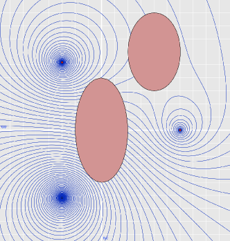
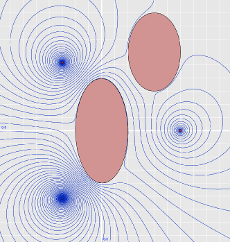
Figure 1: Two bodies surrounded by three point vortices with strengths $1$, $2$, $-3$. The instantaneous fluid motion is along the stream lines (blue), with velocity proportional to the level density. Left: Stream lines of the velocity field $u_{\gamma}$ generated by the point vortices, ignoring the bodies. Right: Stream lines of the velocity field $u_{\|}=u_{\gamma}+u_{I}$. Here the image vorticity makes the fluid flow nicely around the bodies.

We will now construct the fluid velocity field $u$ for a given configuration $(g,\xi,\gamma)$ of $m$ bodies and $n$ point vortices. Here, $g$ and $\xi$ contain the individual body poses $g_{j}$ and motion states $\xi_{j}$, and $\gamma$ encodes the $m$ point vortex positions $\gamma_{i}$. In the absence of bodies, the fluid velocity field whose vorticity is given by the point vortices $\gamma$ with strengths $K$ is determined by the Biot-Savart law:

$$u_{\gamma}(z)=\sum_{i}K_{i}\left(J\frac{\gamma_{i}-z}{\|\gamma_{i}-z\|^{2}}\right),\qquad J=\left(\!\!\begin{array}[]{cc}0&-1\\ 1&0\end{array}\!\!\right).$$ (41)

When bodies are present, the velocity field $u_{\gamma}$ makes fluid particles move across the body boundaries, see Figure 1, left. To fix this, we construct a potential field $u_{I}=\mathop{\mathrm{grad}}\nolimits\phi_{I}$ on $\mathcal{F}$ which compensates the normal flux of $u_{\gamma}$ through the body boundaries, thus satisfying the boundary condition

$${\Big{\langle}}u_{I}(z),n_{j}(z){\Big{\rangle}} =-{\Big{\langle}}u_{\gamma}(z),n_{j}(z){\Big{\rangle}},\text{ for }z\in\partial{\mathcal{B}}_{j}.$$ (42)

The subscript $I$ reflects the fact that $u_{I}$ can be represented as image vorticity inside of the bodies or on their boundaries, see Saffman, (1992, §2.4). The potential $\phi_{I}$ of $u_{I}$ is uniquely determined by the Neumann problem

$$\frac{\partial\phi_{I}}{\partial n}(z) =-{\Big{\langle}}u_{\gamma}(z),n(z){\Big{\rangle}},\text{ for }z\in\partial\mathcal{F}, \Delta\phi_{I}(z) =0, \lim_{z\rightarrow\infty}u_{I}(z) =0.$$ (43)

The superposition $u_{\|}=u_{\gamma}+u_{I}$ satisfies the boundary condition $\langle u_{\|}(z),n(z)\rangle=0$ on $\partial\mathcal{F}$, see Figure 1, right. In other words, it is the correct fluid velocity field as long as the bodies are at rest.

When the bodies move we achieve boundary condition (40) by adding another potential field $u_{\mathcal{B}}=\mathop{\mathrm{grad}}\nolimits\phi_{\mathcal{B}}$, obtained from the Neumann problem

$$\frac{\partial\phi_{\mathcal{B}}}{\partial n}(z) ={\Big{\langle}}\omega_{j}\times z+v_{j},n_{j}(z){\Big{\rangle}},\text{ for }z\in\partial\mathcal{B}_{j}, \Delta\phi_{\mathcal{B}}(z) =0, \lim_{z\rightarrow\infty}u_{\mathcal{B}}(z) =0.$$ (44)

The superposition $u=u_{\gamma}+u_{I}+u_{\mathcal{B}}$ is the unique fluid velocity field which satisfies boundary condition (40), has zero circulation around the individual bodies, vanishes at infinity, and has its’ vorticity field is given by the point vortices $\gamma_{i}$ with strengths $K_{i}$.

The velocity potential $\phi_{\mathcal{B}}$ depends linearly on body velocities $\xi_{j}=(\omega_{j},v_{j})$, due to the linearity of the Neumann problem. Because of (26) it also depends linearly on $\Xi_{j}=(\Omega_{j},V_{j})$, i.e., on velocity in the body frame. We use the notation $\Phi_{\mathcal{B}}$ and $\Phi_{\mathcal{B}_{j}}$ for the corresponding vector-valued potential in body coordinates:

$$\Phi_{\mathcal{B}_{j}}(z) =(\phi_{\mathcal{B}}^{3j}(z),\phi_{\mathcal{B}}^{3j+1}(z),\phi_{\mathcal{B}}^{3j+2}(z))\in\mathbb{R}^{3}, \Phi_{\mathcal{B}}(z) =(\phi_{\mathcal{B}}^{1}(z),\ldots,\phi_{\mathcal{B}}^{3m}(z))\in\mathbb{R}^{3m}.$$

Then we can write $\phi_{\mathcal{B}}$, using the standard inner product, as

$$\phi_{\mathcal{B}}(z) =\sum_{j}{\Big{\langle}}\Phi_{\mathcal{B}_{j}}(z),\Xi_{j}{\Big{\rangle}}={\Big{\langle}}\Phi_{\mathcal{B}}(z),\Xi{\Big{\rangle}}.$$ (45)

Equivalently we can represent the velocity fields $u_{I}$ and $u_{\mathcal{B}}$ in terms of their stream functions $\psi_{I}$ and $\psi_{\mathcal{B}}$. That is:

$$u=\mathop{\mathrm{grad}}\nolimits\phi=J\mathop{\mathrm{grad}}\nolimits\psi.$$

As for the potential $\phi_{\mathcal{B}}$, also $\psi_{\mathcal{B}}$ depends linearly on body velocity. In analogy to (45) we denote the vector-valued stream functions by $\Psi_{\mathcal{B}}$ and $\Psi_{\mathcal{B}_{j}}$:

$$\psi_{\mathcal{B}}(z) =\sum_{j}{\Big{\langle}}\Psi_{\mathcal{B}_{j}}(z),\Xi_{j}{\Big{\rangle}}={\Big{\langle}}\Psi_{\mathcal{B}}(z),\Xi{\Big{\rangle}}.$$ (46)

This representation is important since kinetic energy and the equations of motion are most easily expressed using stream functions.

2.3 Kinetic Energy

The kinetic energy of the fluid velocity field $u$ is

$$\frac{1}{2}\int_{\mathcal{F}}\|u\|^{2}=\frac{1}{2}\int_{\mathcal{F}}\|u_{\|}\|^{2}+\frac{1}{2}\int_{\mathcal{F}}\|u_{\mathcal{B}}\|^{2},$$

since $u_{\|}$ and $u_{\mathcal{B}}$ are $L^{2}$-orthogonal. The kinetic energy associated to $u_{\mathcal{B}}$ can be expressed in terms of added mass as a quadratic form on body velocity, similar to the kinetic energy (29):

$$\frac{1}{2}\int_{\mathcal{F}}\|u_{\mathcal{B}}\|^{2}=\frac{1}{2}{\Big{\langle}}\mathbb{A}(g)\,\Xi,\Xi{\Big{\rangle}}.$$ (47)

The matrix $\mathbb{A}(g)$ is called the added mass tensor, and the main difference to the mass-inertia tensor $\mathbb{M}$ is that $\mathbb{A}(g)$ depends on $g$, while $\mathbb{M}$ is a constant matrix which depends only on the body shapes and mass distributions. For a single rigid body the derivation of (47) goes back to Kirchhoff, (1870), see Nair and Kanso, (2007) for the case of several rigid bodies. Together with the kinetic energy associated to the rigid body motion, we define the Kirchhoff tensor $\mathcal{K}=\mathbb{M}+\mathbb{A}(g)$. The corresponding energy,

$$T_{\mathcal{B}}=\frac{1}{2}{\Big{\langle}}\mathcal{K}\,\Xi,\Xi{\Big{\rangle}},$$ (48)

can be viewed as a function of Kirchhoff momentum $M=\mathcal{K}\Xi$. Then

$$H_{\mathcal{B}}=\frac{1}{2}{\Big{\langle}}M,\mathcal{K}^{-1}M{\Big{\rangle}}$$ (49)

is the Hamiltonian for rigid bodies in potential flow.

The kinetic energy associated to $u_{\|}$ contains infinite self-energy terms that we ignore. The finite part is given as the negative of the Kirchhoff-Routh function $W_{G}$ (Lin,, 1941; Shashikanth,, 2005):

$$W_{G}=\frac{1}{2}\sum_{i}K_{i}\left(\psi_{I}(\gamma_{i})+\sum_{i\neq j}\psi_{\gamma_{j}}(\gamma_{i})\right),$$ (50)

where $\psi_{\gamma_{j}}(z)=-K_{j}\log{\|\gamma_{j}-z\|}$ is the stream function of the point vortex $\gamma_{j}$. In the absence of bodies (or other boundaries) the kinetic energy of $u_{\|}=u_{\gamma}$ reduces to

$$H_{\gamma}=-\frac{1}{2}\sum_{i}K_{i}\sum_{j\neq i}\psi_{\gamma_{j}}(\gamma_{i}),$$ (51)

which is the Hamiltonian of $m$ point vortices in the plane. Note that gradient of $W_{G}$ with respect to a point vortex $\gamma_{i}$ encodes the velocity field $u_{\|}(\gamma_{j})$:

$$\mathop{\mathrm{grad}}\nolimits_{\gamma_{i}}W_{G}=-K_{i}Ju_{\|}(\gamma_{i}).$$ (52)

The total kinetic energy of the coupled system is

$$H=H_{\mathcal{B}}-W_{G}=T_{\mathcal{B}}-W_{G}.$$ (53)

3 Equations of Motion

We consider $m$ rigid bodies (topological disks) in the plane, surrounded by an inviscid and incompressible fluid. The circulation around the individual bodies is zero, and the whole vorticity of the fluid is concentrated at $n$ isolated point vortices $\gamma_{i}\in\mathbb{R}^{2}$, with strengths $K_{i}$. Euclidean transformations and velocity states of the different bodies are denoted by $g_{j}$ and $\Xi_{j}=(\Omega_{j},V_{j})$, as in Section 2.1. We define

$$M_{C} =\sum_{i}K_{i}\Psi_{\mathcal{B}}(\gamma_{i}), W_{\mathcal{B}} =\sum_{i}K_{i}\psi_{\mathcal{B}}(\gamma_{i})={\Big{\langle}}M_{C},\Xi{\Big{\rangle}},$$

and the generalized momentum $M=\mathcal{K}\,\Xi+M_{C}$ with components $M_{j}=(A_{j},L_{j})$ corresponding to angular and linear momentum.

Theorem 1.

The motion of the coupled system described above is governed by the following system of differential equations:

$$\left(\!\!\begin{array}[]{c}\dot{A}_{j}+V_{j}\times L_{j}\\[1.42271pt] \dot{L}_{j}+\Omega_{j}\times L_{j}\end{array}\!\!\right) =-\Big{(}\mathop{\mathrm{lgrad}}\nolimits(H_{\mathcal{B}}-W_{G}-W_{\mathcal{B}})\Big{)}_{j},$$ (54)

$$\Xi =\mathcal{K}^{-1}(M-M_{C}),$$

$$\dot{g}_{j} =g_{j}\Xi_{j},$$

$$\dot{\gamma}_{i} =u(\gamma_{i}).$$

This theorem will be proven in the remainder of this section.

3.1 Hamiltonian Formulation

The starting point for our derivation was made by Vankerschaver et al., (2009), who determined the dynamics of a single, circular disk with point vortices through the framework of cotangent bundle reduction (Marsden et al.,, 2007). Appendix A summarizes the derivation of the reduced phase space for the system. We emphasize here that the derivation readily generalizes to several bodies. Apart from the reduced phase space, one needs to determine the reduced symplectic form in order to fully describe the dynamics. Vankerschaver et al., (2009) use the general framework of cotangent bundle reduction, which determines the symplectic form through the curvature of the mechanical connection. While it is in principle possible to extend this approach to several bodies of arbitrary shape, the derivation requires heavy differential-geometric machinery, takes place in unreduced, infinite-dimensional phase space, and is already challenging for the case of a single, circular disk.

We make use of the fact that the dynamics of the surrounding fluid, and thus the point vortex dynamics, is completely determined from first principles. This allows to determine the symplectic form in finite-dimensional reduced phase space, using standard methods. In particular, we use the fact that point vortices are, by Helmholtz’ law, advected along the fluid velocity field $u$. Further we will show that the dynamics of rigid bodies and point vortices decouples asymptotically. These two properties uniquely determine the symplectic form, and we obtain the equations of motion by computing Hamilton’s equations

$$\sigma(X,\dot{q})=\mathrm{d}H(X),\quad\forall_{X}\in T_{q}{\mathcal{M}}.$$ (55)

Here $\mathcal{M}$ is the reduced phase space, $\sigma$ is the symplectic form, and $H\colon\,{\mathcal{M}}\rightarrow\mathbb{R}$ is the Hamiltonian. The reduced phase space for the coupled system of $n$ bodies and $m$ point vortices is (see Appendix A)

$${\mathcal{M}}=T^{*}\mathrm{SE}(2)^{n}\times\mathbb{R}^{2m},$$ (56)

where $T^{*}\mathrm{SE}(2)^{n}$ is the cotangent bundle of $\mathrm{SE}(2)^{n}$. A point $q=(\mu,g,\gamma)\in{\mathcal{M}}$ encodes body poses $g\in SE(2)^{n}$, body momentum through the covector $\mu\in T_{g}^{*}SE(2)^{n}$, and the $m$ point vortex locations $\gamma\in\mathbb{R}^{2m}$. The two factors of ${\mathcal{M}}$ are already symplectic manifolds, they are the phase spaces of the two uncoupled systems:

• $(T^{*}\mathrm{SE}(2)^{n},\sigma_{can})$ is the phase space of $n$ rigid bodies. Any cotangent bundle carries a canonical symplectic structure, in this case $\sigma_{can}=\mathrm{d}\mu\wedge\mathrm{d}g$. Hamilton’s equations with Hamiltonian $H_{\mathcal{B}}$ (49) describe the motion of $n$ rigid bodies in potential flow.

• $(\mathbb{R}^{2m},\sigma_{\gamma})$ is the phase space of $m$ point vortices in the plane. The symplectic form is $\sigma_{\gamma}=-\sum_{i}K_{i}\mathrm{d}x_{i}\wedge\mathrm{d}y_{i}$, the weighted sum of canonical symplectic forms on the individual $\mathbb{R}^{2}$ factors. Hamilton’s equations with Hamiltonian $H_{\gamma}$ (51) describe the motion of $m$ point vortices in the plane.

We know from general theory of cotangent bundle reduction that the Hamiltonian of the system is the kinetic energy (53), and that the symplectic form $\sigma$ on ${\mathcal{M}}$ is of the form

$$\sigma=\sigma_{can}+\mathrm{d}\alpha+\sigma_{\gamma}.$$ (57)

Here $\sigma_{can}$ and $\sigma_{\gamma}$ are the symplectic forms on the individual factors, and $\mathrm{d}\alpha$ is a magnetic or Coriolis term, which is responsible for the dynamical coupling between rigid bodies and point vortices. The two-form $\mathrm{d}\alpha$ lives on $\mathrm{SE}(2)^{n}\times\mathbb{R}^{2m}$, i.e., it is independent of $\mu$. In the remainder of this section we will determine the magnetic term $\mathrm{d}\alpha$, and then derive the equations of motion (54) from Hamilton’s equations (55).

3.1.1 Asymptotic Decoupling

We will now study the behavior of the coupled dynamical system in the limit when rigid bodies and point vortices are far apart. Assume that both bodies and point vortices are contained in two disjoint disks of finite radius, and let $d$ denote the minimal distance between these disks. We will now show that in the limit $d\rightarrow\infty$ the system decouples:

Lemma 1.

The dynamical system decouples in the limit $d\rightarrow\infty$, i.e.,

$$\lim_{d\rightarrow\infty}\mathrm{d}\alpha=0.$$

Proof.

We consider the difference of Hamilton’s equations of the coupled and the two uncoupled systems. For the difference of the symplectic forms we obtain

$$\sigma-\sigma_{can}-\sigma_{\gamma}=\mathrm{d}\alpha,$$

and the difference of the Hamiltonians is

$$H-H_{\mathcal{B}}-H_{\gamma}=-W_{G}-H_{\gamma}=-\frac{1}{2}\sum_{i}K_{i}\psi_{I}(\gamma_{i}).$$

The difference of Hamilton’s equations in the limit $d\rightarrow\infty$ is

$$\lim_{d\rightarrow\infty}\mathrm{d}\alpha((\Gamma,\delta{\gamma}),(\Xi,\dot{\gamma})) =\lim_{d\rightarrow\infty}\mathrm{d}(H-H_{\mathcal{B}}-H_{\gamma})(\Gamma,\delta{\gamma})$$

$$=\lim_{d\rightarrow\infty}\sum_{i}K_{i}\left(-\frac{1}{2}\delta_{g}\psi_{I}(\gamma_{i})+\langle Ju_{I}(\gamma_{i}),{\delta{\gamma}}_{i}\rangle\right).$$

The right hand side vanishes because of Lemma 2 and the construction of $u_{I}$, see the Equation (43). ∎

It remains to determine the asymptotic behavior of the stream functions $\psi_{I}$, $\psi_{\mathcal{B}}$ and their variations with respect to $g$:

Lemma 2.

The functions $\psi_{I}$, $\psi_{\mathcal{B}}$, $\delta_{g}\psi_{I}$ and $\delta_{g}\psi_{\mathcal{B}}$ are ${\mathcal{O}}(|z|^{-1})$.

Proof.

Let $u$ be $u_{I}$ or $u_{\mathcal{B}}$, and $\psi$ the stream function of $u$. We represent $\psi$ as a single layer potential with density $\tau$, i.e.,

$$\psi(z)= \sum_{j}\nolimits\psi^{j}(z) \psi^{j}(z)= \oint_{\partial\mathcal{B}_{j}}\tau(\eta)\log\|\eta-g_{j}^{-1}(z)\|\,d\eta.$$

Note that we can also view $\tau$ as the strength of a vortex sheet (i.e., a distribution of point vortices) on $\partial\mathcal{B}$, which generates $u$ via the Biot-Savart law (41). Since the circulation of $u=\mathop{\mathrm{grad}}\nolimits\phi$ around any $\mathcal{B}_{j}$ is zero, the total density of $\tau$ on each $\partial\mathcal{B}_{j}$, as well as its variation with respect to $g$, vanish:

$$\oint_{\partial\mathcal{B}_{j}}\tau(\eta)\,d\eta=\oint_{\partial\mathcal{B}_{j}}(\delta_{g}\tau)(\eta)\,d\eta=0.$$ (58)

This implies $\psi^{j}(z)=\psi(z)={\mathcal{O}}(|z|^{-1})$. For the variation with respect to $g$ we obtain

$$\delta_{g}\psi^{j}(z)={\Big{\langle}}\oint_{\partial\mathcal{B}_{j}}\tau(\eta)\frac{\eta-g_{j}^{-1}(z)}{\|\eta-g_{j}^{-1}(z)\|^{2}}\,d\eta,-\delta g_{j}^{-1}(z){\Big{\rangle}}+\oint_{\partial\mathcal{B}_{j}}(\delta_{g}\tau)(\eta)\log\|\eta-g_{j}^{-1}(z)\|\,d\eta.$$

The second term is also a single layer potential and ${\mathcal{O}}(|z|^{-1})$ because of (58). The boundary integral in the first term is a rotated version (by $-\pi/2$) of the velocity field $u$ generated by the single layer density $\tau$ on $\partial\mathcal{B}_{j}$. Thus it is ${\mathcal{O}}(|z|^{-2})$ because of (58), while $\delta g_{j}^{-1}(z)$ is ${\mathcal{O}}(|z|)$. So the first term is ${\mathcal{O}}(|z|^{-1})$ as well. ∎

3.1.2 Dynamics of Hydrodynamically Coupled Rigid Bodies

The dynamics of rigid bodies in potential flow is a canonical Hamiltonian system with phase space ${\mathcal{M}}=T^{*}\mathrm{SE}(2)^{n}$ and Hamiltonian $H_{\mathcal{B}}$, see Equation (49). We use the left trivialization

$$\mathcal{M}=\mathbb{R}^{3n}\times SE(2)^{n}\cong T^{*}\mathrm{SE}(2)^{n}$$ (59)

that is, we identify a covector $\mu\in T_{g}^{*}\mathrm{SE}(2)^{n}$ with its corresponding body momentum $M\in\mathbb{R}^{3n}$. In this way we obtain the equations of motion in the body frame of reference, as an evolution equation for $M$. The canonical symplectic form on $\mathcal{M}$ is derived in Appendix B. Now we compute Hamilton’s equations (55) using the Hamiltonian $H_{\mathcal{B}}$ (49). We have $\dot{q}=(\dot{M},\Xi)$, $X=(\delta M,\Gamma)$, and obtain

$${\Big{\langle}}\delta{M},\Xi{\Big{\rangle}}-{\Big{\langle}}\dot{M}-\mathop{\mathrm{ad}^{*}_{\Xi}}\nolimits M,\Gamma{\Big{\rangle}}={\Big{\langle}}\delta{M},\mathcal{K}^{-1}M{\Big{\rangle}}+{\Big{\langle}}\mathop{\mathrm{lgrad}}\nolimits H_{\mathcal{B}},\Gamma{\Big{\rangle}}.$$

Comparing $\delta{M}$-coefficients gives $M=\mathcal{K}\Xi$ while the $\Gamma$-coefficients give the equations of motion as an evolution equation for $M$:

$$\dot{M}-\mathop{\mathrm{ad}^{*}_{\Xi}}\nolimits M=-\mathop{\mathrm{lgrad}}\nolimits H_{\mathcal{B}}\qquad\Longleftrightarrow\qquad\left(\!\!\begin{array}[]{c}\dot{A}_{j}+V_{j}\times L_{j}\\ \dot{L}_{j}+\Omega_{j}\times L_{j}\end{array}\!\!\right)=-\big{(}\mathop{\mathrm{lgrad}}\nolimits H_{\mathcal{B}}\big{)}_{j}.$$

3.1.3 Point Vortex Dynamics

According to Helmholtz’ law (see, for instance, Saffman, (1992)), point vortices are frozen into the fluid velocity field: $\dot{\gamma}_{i}=u(\gamma_{i})$. The Hamiltonian formulation of the system is obtained as follows. The symplectic form for $m$ point vortices $\gamma\in\mathbb{R}^{2m}$ with strengths $K_{i}$ is

$$\sigma_{\gamma}=-\sum_{i}K_{i}\,\mathrm{d}x_{i}\wedge\mathrm{d}y_{i},\quad\text{ i.e., }\quad\sigma_{\gamma}(\delta{\gamma},\dot{\gamma})=\sum_{i}K_{i}{\Big{\langle}}\delta{\gamma}_{i},J\dot{\gamma}_{i}{\Big{\rangle}}.$$

In the absence of boundaries the Hamiltonian is $H_{\gamma}$ (51). Computing Hamilton’s equations,

$$\sigma_{\gamma}(\delta{\gamma},\dot{\gamma})=\mathrm{d}H_{\gamma}(\delta{\gamma})\qquad\Longleftrightarrow\qquad\sum_{i}K_{i}{\Big{\langle}}{\delta{\gamma}}_{i},J\dot{\gamma}_{i}{\Big{\rangle}}=\sum_{i}K_{i}{\Big{\langle}}Ju_{\gamma}(\gamma_{i}),{\delta{\gamma}}_{i}{\Big{\rangle}},$$

we obtain, as expected, $\dot{\gamma}_{i}=u_{\gamma}(\gamma_{i})$. This holds also for a fluid with fixed boundaries, i.e., for fixed body configuration. In this case we can choose the negative of the Kirchhoff-Routh function $-W_{G}$ (Equation (50)) as the Hamiltonian and obtain $\dot{\gamma}_{i}=u_{\|}(\gamma_{i})$. In both cases the Hamiltonian is the kinetic energy of the fluid velocity field (with infinite self-energy terms excluded), and the Hamiltonian is a constant of motion.

In the case of rigidly moving boundaries we use the generalized Kirchhoff-Routh function, extended to rigidly moving boundaries by Shashikanth et al., (2002):

$$W=W_{G}+W_{\mathcal{B}},\quad W_{\mathcal{B}}=\sum_{i}K_{i}\psi_{\mathcal{B}}(\gamma_{i}).$$ (60)

Choosing $-W$ as the Hamiltonian gives the correct point vortex dynamics for the case that some agency moves the bodies around. Here the Hamiltonian depends explicitly on time, thus it is not a constant of motion.

3.1.4 Dynamics of the Coupled System

Looking at the dynamics of point vortices in a fluid with rigidly moving boundaries (Section 3.1.3), it is not surprising that the function $W_{\mathcal{B}}$ (60) needs to make its way into Hamilton’s equations of the coupled system. However, the Hamiltonian of the system is already known: It is the kinetic energy $H=-W_{G}+H_{\mathcal{B}}$ of the combined fluid-body system, given in Equation (53). On the other hand, $W_{\mathcal{B}}$ can be viewed as a one-form on $\mathrm{SE}(2)^{n}\times\mathbb{R}^{2m}$. We will now show that $\alpha=W_{\mathcal{B}}$ is in fact a primitive of the magnetic term $\mathrm{d}\alpha$.

Lemma 3.

The one-form

$$\alpha(\Xi,\dot{\gamma}) :=W_{\mathcal{B}}={\Big{\langle}}M_{C},\Xi{\Big{\rangle}}, M_{C} =\sum_{i}K_{i}\Psi_{\mathcal{B}}(\gamma_{i})$$ (61)

on $\mathrm{SE}(2)^{n}\times\mathbb{R}^{2m}$ is a primitive one-form of the magnetic term $\mathrm{d}\alpha$.

Proof.

Let us compute Hamilton’s equations for the coupled system, i.e.,

$$\sigma\left(X,\dot{q}\right)=\mathrm{d}H(X),$$ (62)

with $\dot{q}=(\dot{M},\Xi,\dot{\gamma})$ and $X=(\delta{M},\Gamma,\delta{\gamma})$ is an arbitrary tangent vector at $q=(M,g,\gamma)$:

$$\mathrm{d}H(X) ={\Big{\langle}}\delta{M},\mathcal{K}^{-1}M{\Big{\rangle}}+{\Big{\langle}}\mathop{\mathrm{lgrad}}\nolimits_{g}H,\Gamma{\Big{\rangle}}+\sum_{i}K_{i}{\Big{\langle}}Ju_{\|}(\gamma_{i}),{\delta{\gamma}}_{i}{\Big{\rangle}},$$ (63)

$$\sigma(X,\dot{q}) ={\Big{\langle}}\delta{M},\Xi{\Big{\rangle}}-{\Big{\langle}}\dot{M}-\mathop{\mathrm{ad}^{*}_{\Xi}}\nolimits M,\Gamma{\Big{\rangle}}+\sigma_{\gamma}(X,\dot{\gamma})+\mathrm{d}\alpha\left((\Gamma,\delta{\gamma}),(\Xi,\dot{\gamma})\right).$$

From the $\delta{M}$-coefficients we immediately obtain $M=\mathcal{K}\Xi$. Further, using the linearity of $\mathrm{d}\alpha$ with respect to $(\Gamma,\delta{\gamma})$, we have

$$\sigma_{\gamma}(\delta{\gamma},\dot{\gamma})+\mathrm{d}\alpha((0,\delta{\gamma}),(\Xi,\dot{\gamma}))=\sum_{i}K_{i}{\Big{\langle}}Ju_{\|}(\gamma_{i}),{\delta{\gamma}}_{i}{\Big{\rangle}}.$$ (64)

By virtue of Helmholtz’ law point vortices are frozen into the fluid, i.e., $\dot{\gamma}_{i}=u(\gamma_{i})$. Therefore we can rewrite the right hand side using $u_{\|}=u-u_{\mathcal{B}}$ and obtain

$$\sum_{i}K_{i}{\Big{\langle}}Ju_{\|}(\gamma_{i}),{\delta{\gamma}}_{i}{\Big{\rangle}} =\sum_{i}K_{i}{\Big{\langle}}J(\dot{\gamma}_{i}-u_{\mathcal{B}}(\gamma_{i})),{\delta{\gamma}}_{i}{\Big{\rangle}}$$

$$=\sigma_{\gamma}(\delta{\gamma},\dot{\gamma})+{\Big{\langle}}\mathop{\mathrm{grad}}\nolimits_{\gamma}W_{\mathcal{B}},\delta{\gamma}{\Big{\rangle}}=\sigma_{\gamma}(\delta{\gamma},\dot{\gamma})+{\Big{\langle}}\mathop{\mathrm{grad}}\nolimits_{\gamma}\langle M_{C},\Xi\rangle,\delta{\gamma}{\Big{\rangle}}.$$

Subtracting $\sigma_{\gamma}$ on both sides of (64) we have

$$\mathrm{d}\alpha\left((0,\delta{\gamma}),(\Xi,\dot{\gamma})\right)={\Big{\langle}}\mathop{\mathrm{grad}}\nolimits_{\gamma}\langle M_{C},\Xi\rangle,\delta{\gamma}{\Big{\rangle}}.$$ (65)

From the general theory of cotangent-bundle reduction we know that $\mathrm{d}\alpha$ does not dependent on $M$. In particular, we can consider $M=0$ which implies $\Xi=0$ and thus verify that $\mathrm{d}\alpha\left((0,\delta{\gamma}),(0,\dot{\gamma})\right)=0$. As a consequence, we can assume $\alpha$ to be of the form

$$\alpha(\Xi,\dot{\gamma})={\Big{\langle}}M_{\alpha}(g,\gamma),\Xi{\Big{\rangle}}.$$

We compute $\mathrm{d}\alpha$ and obtain

$$\mathrm{d}\alpha((\Gamma,\delta{\gamma}),(\Xi,\dot{\gamma})) =\delta{\Big{\langle}}{M}_{\alpha},\Xi{\Big{\rangle}}-{\Big{\langle}}{M}_{\alpha},\Gamma{\Big{\rangle}}\dot{}$$ (66)

$$={\Big{\langle}}\mathop{\mathrm{lgrad}}\nolimits\langle M_{\alpha},\Xi\rangle,\Gamma{\Big{\rangle}}+{\Big{\langle}}\mathop{\mathrm{grad}}\nolimits_{\gamma}\langle M_{\alpha},\Xi\rangle,\delta\gamma{\Big{\rangle}}-{\Big{\langle}}\dot{M}_{\alpha}-\mathop{\mathrm{ad}^{*}_{\Xi}}\nolimits M_{\alpha},\Gamma{\Big{\rangle}}.$$

When equating (65) and (66) (for $\Gamma=0$) we obtain

$$\mathop{\mathrm{grad}}\nolimits_{\gamma}{\Big{\langle}}M_{\alpha},\Xi{\Big{\rangle}}=\mathop{\mathrm{grad}}\nolimits_{\gamma}{\Big{\langle}}M_{C},\Xi{\Big{\rangle}}.$$

This determines $M_{\alpha}$ up to a contribution that is independent of $\gamma$, i.e., $M_{\alpha}=M_{C}+\tilde{M}(g)$. It remains to be shown that $\tilde{M}$ does not contribute to $\mathrm{d}\alpha$. Let us write $\alpha=\hat{\alpha}+\tilde{\alpha}$ with

$$\hat{\alpha}(\Xi,\dot{\gamma}) ={\Big{\langle}}M_{C},\Xi{\Big{\rangle}}, \tilde{\alpha}(\Xi,\dot{\gamma}) ={\Big{\langle}}\tilde{M},\Xi{\Big{\rangle}}.$$

When we consider the limit $d\rightarrow\infty$ (distance between point vortices and bodies), it follows from Lemma 2 that $\lim_{d\rightarrow\infty}\mathrm{d}\hat{\alpha}=0$. Lemma 1 on the other hand guarantees that the system decouples in this limit, i.e., $\lim_{d\rightarrow\infty}\mathrm{d}\alpha=0$. It follows that $\mathrm{d}\tilde{\alpha}$ vanishes identically, since it is independent of $\gamma$, and thus of $d$. ∎

Now we are able to verify the equations of motion given in Theorem 1:

Proof of Theorem 1.

The magnetic term is (see Equation (66), with $M_{\alpha}=M_{C}$)

$$\mathrm{d}\alpha ={\Big{\langle}}\mathop{\mathrm{lgrad}}\nolimits W_{\mathcal{B}},\Gamma{\Big{\rangle}}-\sum_{i}K_{i}{\Big{\langle}}Ju_{\mathcal{B}}(\gamma_{i}),\delta\gamma_{i}{\Big{\rangle}}-{\Big{\langle}}\dot{M}_{C}-\mathop{\mathrm{ad}^{*}_{\Xi}}\nolimits M_{C},\Gamma{\Big{\rangle}}.$$

Substituting into Hamilton’s equations ((62) and (63)) and bringing the first two terms to the right hand side gives

$$RHS ={\Big{\langle}}\delta{M},\mathcal{K}^{-1}M{\Big{\rangle}}+{\Big{\langle}}\mathop{\mathrm{lgrad}}\nolimits_{g}(H_{\mathcal{B}}-W),\Gamma{\Big{\rangle}}+\sum_{i}K_{i}{\Big{\langle}}Ju(\gamma_{i}),{\delta{\gamma}}_{i}{\Big{\rangle}},$$

$$LHS ={\Big{\langle}}\delta M,\Xi{\Big{\rangle}}-{\Big{\langle}}(\dot{M}+\dot{M}_{C})-\mathop{\mathrm{ad}^{*}_{\Xi}}\nolimits(M+M_{C}),\Gamma{\Big{\rangle}}+\sum_{i}K_{i}{\Big{\langle}}J\dot{\gamma}_{i},\delta{\gamma}_{i}{\Big{\rangle}}.$$

Comparing coefficients gives the equations of motion (54). ∎

4 Lagrangian Formulation and Total Momentum

For any canonical Hamiltonian system on a cotangent bundle $\mathcal{M}=T^{*}\mathcal{Q}$ with canonical symplectic form $\sigma=\mathrm{d}\Theta$, a Lagrangian description is obtained through the Legendre transformation. That is, momentum is expressed as a function on the tangent bundle $T\mathcal{Q}$, and the Lagrangian is $L=\Theta-H$, also viewed as a function on $T\mathcal{Q}$. The corresponding Euler-Lagrange equations give the same dynamics as the Hamiltonian system, a classical result which can be found in any mechanics textbook.

The above construction does not apply to point vortices, since the phase space is not a cotangent bundle, and it is thus not clear (and in general not even possible) how to split this space into configurations and momenta. Nevertheless, if $\beta_{\gamma}$ is a primitive for $\sigma_{\gamma}=\mathrm{d}\beta_{\gamma}$, one can show that the Lagrangian $L=\beta_{\gamma}-H_{\gamma}$ describes the dynamics of point vortices, see Rowley and Marsden, (2002). We will now verify that this approach also gives a Lagrangian description for the coupled dynamics of rigid bodies and point vortices.

A primitive one-form of $\sigma=\sigma_{can}+\sigma_{\gamma}+\mathrm{d}\alpha$ is easily found: The canonical symplectic form on $T^{*}\mathrm{SE}(2)^{n}$ is the exterior derivative of $\beta_{can}=\langle M,\Xi\rangle=\langle\mathcal{K}\Xi,\Xi\rangle$, see Appendix B. For $\sigma_{\gamma}$ we use the primitive

$$\beta_{\gamma}=-\frac{1}{2}\sum_{i}K_{i}\det(\gamma_{i},\dot{\gamma}_{i})=-\frac{1}{2}\sum_{i}K_{i}{\Big{\langle}}\gamma_{i},J\dot{\gamma}_{i}{\Big{\rangle}}.$$

With $\alpha=W_{\mathcal{B}}=\langle M_{C},\Xi\rangle$ obtain as the Lagrangian

$$L =\beta-H=\underbrace{{\Big{\langle}}\mathcal{K}\Xi,\Xi{\Big{\rangle}}}_{2T_{\mathcal{B}}}+\beta_{\gamma}+W_{\mathcal{B}}-T_{\mathcal{B}}+W_{G}=T_{\mathcal{B}}+\beta_{\gamma}+W,$$ (67)

where we have expressed the Kirchhoff kinetic energy $H_{\mathcal{B}}$ as a function on the tangent bundle, denoted by $T_{\mathcal{B}}$. We will now verify that $L$ is indeed a Lagrangian for the system. At the same time we will determine the total momentum of the system, by keeping track of the end points when using integration by parts:

$$0=\delta S_{L} =\delta\int_{t_{0}}^{t_{1}}L\,dt=\int_{t_{0}}^{t_{1}}\delta\beta_{\gamma}+\delta(T_{\mathcal{B}}+W)\,dt$$

$$=\int_{t_{0}}^{t_{1}}{\Big{\langle}}\mathop{\mathrm{lgrad}}\nolimits(T_{\mathcal{B}}+W),\Gamma{\Big{\rangle}}+{\Big{\langle}}\underbrace{\mathcal{K}\Xi+M_{C}}_{M},\delta\Xi{\Big{\rangle}}\,dt$$

$$+\sum_{i}K_{i}\int_{t_{0}}^{t_{1}}\frac{1}{2}{\Big{\langle}}\delta\gamma_{i},J\dot{\gamma}_{i}{\Big{\rangle}}+\frac{1}{2}{\Big{\langle}}\gamma_{i},J\delta\dot{\gamma}_{i}{\Big{\rangle}}-{\Big{\langle}}Ju(\gamma_{i}),\delta\gamma_{i}{\Big{\rangle}}\,dt.$$

Now we use $\delta\Xi=\dot{\Gamma}+\mathop{\mathrm{ad}_{\Xi}}\nolimits\Gamma$ (see Equation (74) in Appendix B) and integration by parts, i.e.,

$${\Big{\langle}}M,\Gamma{\Big{\rangle}}\Big{|}_{t_{0}}^{t_{1}} =\int_{t_{0}}^{t_{1}}{\Big{\langle}}\dot{M},\Gamma{\Big{\rangle}}+{\Big{\langle}}M,\dot{\Gamma}{\Big{\rangle}}\,dt,$$

$$\frac{1}{2}{\Big{\langle}}\gamma_{i},J\delta{\gamma}_{i}{\Big{\rangle}}\Big{|}_{t_{0}}^{t_{1}} =\frac{1}{2}\int_{t_{0}}^{t_{1}}{\Big{\langle}}\dot{\gamma}_{i},J\delta\gamma_{i}{\Big{\rangle}}+{\Big{\langle}}\gamma_{i},\delta\dot{\gamma}_{i}{\Big{\rangle}}\,dt,$$

and obtain

$$\delta S_{L} =\int_{t_{0}}^{t_{1}}{\Big{\langle}}\mathop{\mathrm{lgrad}}\nolimits(T_{\mathcal{B}}+W)+\mathop{\mathrm{ad}^{*}_{\Xi}}\nolimits M-\dot{M},\Gamma{\Big{\rangle}}+\sum_{i}K_{i}{\Big{\langle}}J(\dot{\gamma}_{i}-u(\gamma_{i})),\delta\gamma_{i}{\Big{\rangle}}\,dt$$

$$+\left({\Big{\langle}}M,\Gamma{\Big{\rangle}}+\frac{1}{2}\sum_{i}K_{i}{\Big{\langle}}\gamma_{i},J\delta\gamma_{i}{\Big{\rangle}}\right)\Big{|}_{t_{0}}^{t_{1}}.$$

For variations with fixed end points we obtain the equations of motion (Theorem 1) as critical values of $S_{L}$. The Euler-Lagrange equations of the system are

$$\mathop{\mathrm{lgrad}}\nolimits(T_{\mathcal{B}}+W)+\mathop{\mathrm{ad}^{*}_{\Xi}}\nolimits M-\dot{M} =0, \dot{\gamma}_{i}-u(\gamma_{i}) =0.$$ (68)

Since $\mathop{\mathrm{lgrad}}\nolimits T_{\mathcal{B}}=-\mathop{\mathrm{lgrad}}\nolimits H_{\mathcal{B}}$ we have proven:

Corollary 1.

The function $L=T_{\mathcal{B}}+\beta_{\gamma}+W$ is a Lagrangian for the coupled system of rigid bodies and point vortices.

The total momentum of the system is obtained by applying an infinitesimal Euclidean motion to a solution $q$ of the Euler-Lagrange equations. The corresponding variation $\delta q$ has the form

$$\delta g_{j} =\underbrace{\left(\!\!\begin{array}[]{cc}\tilde{\omega}\times&\tilde{v}\\ 0&0\end{array}\!\!\right)}_{c}g_{j}=g_{j}\Gamma_{j}, \delta\gamma_{i}=\tilde{\omega}\times\gamma_{i}+\tilde{v}.$$

Since $q$ solves the Euler-Lagrange equations (68) we obtain

$$\delta S_{L}=\left(\sum_{j}{\Big{\langle}}M_{j},\mathop{\mathrm{Ad}_{g_{j}^{-1}}}\nolimits c{\Big{\rangle}}+\frac{1}{2}\sum_{i}K_{i}{\Big{\langle}}\gamma_{i},J\delta\gamma_{i}{\Big{\rangle}}\right)\Big{|}_{t_{0}}^{t_{1}}.$$ (69)

On the other hand, $T_{\mathcal{B}}+W$ does not change under a Euclidean motion. Hence

$$\delta S_{L} =\int_{t_{0}}^{t_{1}}\delta\beta_{\gamma}\,dt=\frac{1}{2}\sum_{i}K_{i}\int_{t_{0}}^{t_{1}}{\Big{\langle}}\delta\gamma_{i},J\dot{\gamma}_{i}{\Big{\rangle}}+{\Big{\langle}}\gamma_{i},J\delta\dot{\gamma}_{i}{\Big{\rangle}}\,dt$$ (70)

$$=\sum_{i}K_{i}\int_{t_{0}}^{t_{1}}{\Big{\langle}}\delta\gamma_{i},J\dot{\gamma}_{i}{\Big{\rangle}}\,dt+\frac{1}{2}\sum_{i}K_{i}{\Big{\langle}}\gamma_{i},J\delta{\gamma}_{i}{\Big{\rangle}}\Big{|}_{t_{0}}^{t_{1}}$$

$$={\Big{\langle}}\sum_{i}K_{i}\left(\!\!\begin{array}[]{c}\frac{1}{2}\|\gamma_{i}\|^{2}\\ J\gamma_{i}\end{array}\!\!\right),\left(\!\!\begin{array}[]{c}\tilde{\omega}\\ \tilde{v}\end{array}\!\!\right){\Big{\rangle}}\Big{|}_{t_{0}}^{t_{1}}+\frac{1}{2}\sum_{i}K_{i}{\Big{\langle}}\gamma_{i},J\delta{\gamma}_{i}{\Big{\rangle}}\Big{|}_{t_{0}}^{t_{1}}.$$

Here we have again used integration by parts and the fact that

$${\Big{\langle}}\frac{d}{dt}\Big{|}_{t=0}\left(\!\!\begin{array}[]{c}\frac{1}{2}\|\gamma_{i}\|^{2}\\ J\gamma_{i}\end{array}\!\!\right),\left(\!\!\begin{array}[]{c}\tilde{\omega}\\ \tilde{v}\end{array}\!\!\right){\Big{\rangle}}={\Big{\langle}}\delta\gamma_{i},J\dot{\gamma}_{i}{\Big{\rangle}}.$$

The total momentum is obtained by equating (69) and (70), and using the fact that this equation holds for any $t_{1}$:

Corollary 2.

The coupled system of rigid bodies and point vortices has the following constants of motion induced by the Euclidean symmetry group:

$$const. =\sum_{j}\left(\!\!\begin{array}[]{c}a_{j}\\ \ell_{j}\end{array}\!\!\right)-\sum_{i}K_{i}\left(\!\!\begin{array}[]{c}\frac{1}{2}\|\gamma_{i}\|^{2}\\ J\gamma_{i}\end{array}\!\!\right), \left(\!\!\begin{array}[]{c}a_{j}\\ \ell_{j}\end{array}\!\!\right) =\mathop{\mathrm{Ad}^{*}_{g_{j}^{-1}}}\nolimits M_{j}=\left(\!\!\begin{array}[]{c}A_{j}y_{j}\times R_{j}L_{j}\\ R_{j}L_{j}\end{array}\!\!\right).$$

5 Numerical Simulation

In this section we briefly describe how to implement a numerical method to simulate the dynamics of the coupled system, and validate our method by simulating different configurations.

We have chosen to construct a variational integrator Marsden and West, (2001) for the system, based on the Lagrangian formulation given in Section 4. The Lagrangian of the system is partly degenerate, so it fits into the framework of variational integrators for degenerate Lagrangian systems, see Rowley and Marsden, (2002). Some aspects of implementation regarding the Lie group configuration space can be found in (Kobilarov et al.,, 2009).

Our implementation uses a midpoint scheme, i.e., we discretize the smooth action integral by evaluating in between two configurations (along a geodesic connecting them), and multiplying the corresponding value with the time step:

$$L^{d}(q_{k},q_{k+1})=hL\left((q,\dot{q})\big{|}_{k+\frac{1}{2}}\right).$$

Here the indices correspond to the discrete time evolution. The discrete time evolution is then obtained by subsequently solving the discrete Euler-Lagrange equations

$$D_{2}L^{d}(q_{k-1},q_{k})+D_{1}L^{d}(q_{k},q_{k+1})=0,$$

for $q_{k+1}$, with $q_{k-1}$ and $q_{k}$ known. In order to evaluate the Lagrangian $L$ (67) we discretize the system as follows: We replace the smooth body boundaries by polygons, and represent the potential fields $u_{I}$ and $u_{\mathcal{B}}$ using point sources, which are attached to the rigid bodies. This discretization has previously been used to compute the Kirchhoff tensor of 3D bodies (Weißmann and Pinkall,, 2012). This allows to explicitly compute all quantities and variations needed for evaluating the discrete Euler-Lagrange equations, and we have implemented a numerical scheme in this way. For validation we have simulated the following configurations:

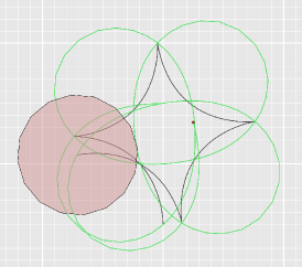
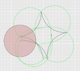
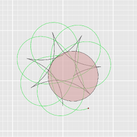
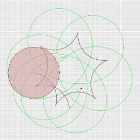
Figure 2: Interaction of a unit disk with one point vortex. Top: The two figures show the simulation of the same initial setup, but with different time step (0.025 vs. 0.25) and body discretization (16 vs. 64 edges). Note that the overall structure is identical, even though both discretization and time step are very different. Bottom: Simulations with a light (density 0.1) and a heavy (density 4.0) disk. Mass affects the frequency of the periodic motion.

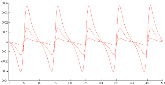
Figure 3: Energy oscillation of the disk-vortex interaction. The three plots correspond to time steps 0.025, 0.1 and 0.25. Note that the oscillations agree precisely, but the magnitude is proportional to the time step.

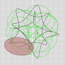
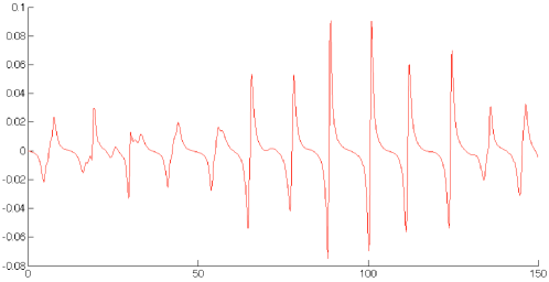
Figure 4: Interaction of a point vortex with an ellipse, with time step 0.1. The motion is chaotic, in contrast to disk/vortex interaction. The plot shows energy oscillations. Large peeks correspond to high dynamical interaction, when body and point vortex are close together.

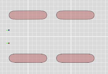
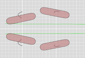
Figure 5: Fluid flow inside of a channel, initial configuration (left) and configuration after the vortex pair has traveled through the channel (right). Because of the higher velocity the pressure is lower in between the walls (Bernoulli’s principle), dragging them together.

Disk with single point vortex: This case is particularly interesting, since it is one of the rare cases where fluid-body interaction is integrable (Borisov and Mamaev,, 2003). The system has periodic (and even closed) orbits, i.e., disk and vortex “dance” around each other, producing a regular, periodic pattern. The mass of the disk determines the frequency of the oscillating motion. Different motions are shown in Figure 2.

Ellipse with single point vortex: This case can be viewed as a distortion of the integrable case of a disk. However, this small change drastically changes the behavior of the system: There are no closed orbits and the motion is chaotic, see Figure 4.

Flow through a channel: This configuration (Figure 5) illustrates Bernoulli’s principle, i.e., pressure is low in regions of high velocity. A vortex pair travels through a channel made out of four flat objects. Due to higher velocity in between the walls are pulled together.

All simulations preserve linear and angular momentum (in the absence of external forces) up to the precision used when solving the discrete Euler-Lagrange equations. The total energy of the system oscillates around its true value during the simulations. The magnitude of these oscillations appears to be proportional to the chosen time step (Figure 3), while the body discretization has no significant influence. These oscillations can be large at times of high dynamical interaction, i.e., when the vortices are very close to the bodies. Nevertheless there is no drift, only oscillations around the true energy level (Figure 4, right). All simulations were computed on a Macbook Pro with a 2.7 GHz Intel Core i7 and 16 GB RAM. The implementation is done in Matlab, and uses no performance optimization such as GPU computations. Configurations with one body take about 0.5 s per time step, the channel example (Figure 5) with 4 bodies around 30 s per time step.

6 Conclusions and Outlook

We have introduced the Hamiltonian description for several rigid bodies interacting with point vortices, assuming zero circulation around the individual bodies, but arbitrary point vortex strengths. We have used the general framework of cotangent bundle reduction only to determine the reduced phase space of the system, as well as the general structure of the symplectic form on the reduced phase space. From there we have determined the symplectic form directly, without resorting to the abstract framework of mechanical connections. From the Hamiltonian formulation we have given a Lagrangian description of the dynamics, and derived a variational time integrator following Marsden and West, (2001) and Rowley and Marsden, (2002). Using polygonal bodies and point sources, we have implemented a numerical algorithm to simulate the coupled dynamics and validated the implementation with different configurations.
We expect that our formulation generalizes to the 3D case, describing the dynamics of several rigid bodies interacting with vortex filaments. So far the dynamics is only known for the case of a single rigid body (Shashikanth et al.,, 2008).

Acknowledgment: Ulrich Pinkall proposed the basic idea for deriving the symplectic form. It is my great pleasure to thank him for invaluable discussions and suggestions. Felix Knöppel and David Chubelaschwili helped working out many of the details. Eva Kanso and the anonymous reviewers provided important feedback for improving the exposition. This work is supported by the DFG Research Center Matheon and the SFB/TR 109 “Discretization in Geometry and Dynamics”.

Appendix A Cotangent Bundle Reduction of Fluid-Body Dynamics

In analogy to Arnold’s geometric description of fluid dynamics (Arnold,, 1966), the dynamics of rigid bodies interacting with a surrounding incompressible fluid can be viewed as a geodesic problem on a Riemannian manifold. The kinetic energy defines a Riemannian metric on the configuration space, and geodesics satisfy Hamilton’s equations on the cotangent bundle with kinetic energy as the Hamiltonian. This insight is due to Vankerschaver et al., (2009) (VKM). The authors use the framework of cotangent bundle reduction (Marsden et al.,, 2007) to obtain a reduced Hamiltonian system with magnetic symplectic form for the case of a single body in a fluid whose vorticity field is concentrated at point vortices.

The Hamiltonian formulation by VKM is an extension of Arnold’s original work (Arnold,, 1966), which describes the motion of an incompressible inviscid fluid in a fixed fluid domain $\mathcal{F}$ as a geodesic on the group $\mathop{\mathrm{Diff}}\nolimits_{\mathop{\mathrm{vol}}\nolimits}(\mathcal{F})$ of volume-preserving diffeomorphisms on $\mathcal{F}$. However, when the fluid interacts with rigid bodies, the fluid domain is no longer fixed. The idea of VKM is to consider the space $\mathop{\mathrm{Emb}}\nolimits_{\mathop{\mathrm{vol}}\nolimits}(\mathcal{F}^{0},\mathbb{R}^{2})$ of volume-preserving embeddings of an initial reference configuration $\mathcal{F}^{0}$ into $\mathbb{R}^{2}$ instead of $\mathop{\mathrm{Diff}}\nolimits_{\mathop{\mathrm{vol}}\nolimits}(\mathcal{F})$. Any incompressible fluid motion is then described by a curve in the subset $\mathcal{Q}^{\mathcal{F}}\subset\mathop{\mathrm{Emb}}\nolimits_{\mathop{\mathrm{vol}}\nolimits}(\mathcal{F}^{0},\mathbb{R}^{2})$ which is compatible with the body motion. The configuration space of the coupled system is $\mathcal{Q}=\mathrm{SE}(2)^{n}\times\mathcal{Q}^{\mathcal{F}}$, and the dynamics is a canonical Hamiltonian system on $T^{*}\mathcal{Q}$ with kinetic energy as the Hamiltonian.

The kinetic energy is invariant under volume-preserving diffeomorphisms of the initial fluid configuration $\mathcal{F}^{0}$ (particle relabeling symmetry), i.e., the symmetry group $\mathop{\mathrm{Diff}}\nolimits_{\mathop{\mathrm{vol}}\nolimits}(\mathcal{F}^{0})$ acts from the right on $\mathcal{Q}^{\mathcal{F}}$, and thus on $\mathcal{Q}$. This action turns $\mathcal{Q}$ into a principal fiber bundle over $\mathrm{SE}(2)^{n}$. This structure allows to follow the famous Kaluza-Klein approach to determine the Hamiltonian dynamics. In order to factor out the $\mathop{\mathrm{Diff}}\nolimits_{\mathop{\mathrm{vol}}\nolimits}(\mathcal{F}^{0})$-symmetry one needs to fix a value of the associated momentum map, which corresponds to choosing an initial vorticity field of the fluid. This is where the assumption is used that vorticity is concentrated at $m$ point vortices. The reduced phase space is $\mathcal{M}=T^{*}SE(2)^{n}\times\mathbb{R}^{2m}$, see VKM, § 4.2, and the dynamics is given by a reduced symplectic form $\sigma$ on $\mathcal{M}$ with kinetic energy as the Hamiltonian. The following theorem formulates the starting point for the derivations made in this paper.

Theorem 2.

The dynamics of $n$ rigid bodies interacting with $m$ isolated point vortices is a Hamiltonian system. The Hamiltonian is the kinetic energy (53), and the phase space is

$$\mathcal{M}=T^{*}\mathrm{SE}(2)^{n}\times\mathbb{R}^{2m}.$$

The cotangent bundle $T^{*}\mathrm{SE}(2)^{n}$ corresponds to the rigid body configuration, and $\mathbb{R}^{2m}$ is the phase space for $m$ point vortices. The symplectic form is

$$\sigma=\sigma_{can}+\mathrm{d}\alpha+\sigma_{\gamma},$$

where $\sigma_{can}$ is the canonical symplectic form on the cotangent bundle $T^{*}\mathrm{SE}(2)^{n}$, $\sigma_{\gamma}$ is the Kirillov-Kostant-Sariou form on the coadjoint orbit $\mathbb{R}^{2n}$, and and $\mathrm{d}\alpha$ is a magnetic term, i.e., a two-form on $SE(2)^{n}\times\mathbb{R}^{2m}$.

Proof.

This has been proven in VKS, §4. We emphasize here that the proofs do not rely on the fact that only a single rigid body was considered. ∎

Appendix B The Cotangent Bundle of Euclidean Motions

In this section we consider the Lie group of Euclidean motions $\mathrm{SE}(2)$ and denote the pairing between covectors and vectors by $\left(.,.\right)$. For any covector $\mu\in T_{g}^{*}\mathrm{SE}(2)$ we can find a body momentum $M\in\mathbb{R}^{3}\cong\mathfrak{se}^{*}(2)$ such that $\left(\mu,\delta g\right):=\langle M,\Lambda\rangle$, for any $\delta g=g\Lambda$. Note that $\Theta(\delta\mu,\delta g):=\left(\mu,\delta g\right)$ is a one-form on the contangent bundle $T^{*}\mathrm{SE}(2)$, and $\langle M,\Lambda\rangle$ is its push-forward to the left trivialization $\mathbb{R}^{3}\times\mathrm{SE}(2)\cong T^{*}\mathrm{SE}(2)$. It is the canonical one-form, and its exterior derivative gives the canonical symplectic form on $T^{*}\mathrm{SE}(2)$. We will now compute the symplectic form when pushed forward to the left trivialization $\mathbb{R}^{3}\times\mathrm{SE}(2)$, using the general formula for the exterior derivative of a one-form:

$$\mathrm{d}\Theta(X,Y)=\nabla_{X}\Theta(Y)-\nabla_{Y}\Theta(X)-\Theta([X,Y]).$$ (71)

Here $X$ and $Y$ are vector fields and $[X,Y]$ is the Jacobi-Lie bracket of $X$ and $Y$. Consider a two-parameter family $(M(s,t),g(s,t))$ in $\mathbb{R}^{3}\times\mathrm{SE}(2)$, whose partial derivatives (denoted by $\delta$ and ^′, respectively) commute. The vector fields will be $X=(\delta M,\delta g)$ and $Y=(M^{\prime},g^{\prime})$, where $\delta g=g\Gamma$ and $g^{\prime}=g\Xi$ with $\Xi=(\Omega,V)$. One can check that the partial derivatives of $g$ commute if and only if

$$\Gamma^{\prime} =\delta\Xi-\mathop{\mathrm{ad}_{\Xi}}\nolimits\Gamma, \mathop{\mathrm{ad}_{\Xi}}\nolimits =\left(\!\!\begin{array}[]{cc}0&0\\ V\times&\Omega\times\end{array}\!\!\right).$$ (74)

The commuting partial derivatives ensure that the Jacobi-Lie bracket in (71) vanishes. The covariant derivatives are usual directional derivatives here, so we obtain the canonical symplectic two–form $\sigma=\mathrm{d}\Theta$ in the left-trivialization as

$$\sigma\left((\delta M,\Gamma),(M^{\prime},\Xi)\right)=\delta{{\Big{\langle}}M,\Xi{\Big{\rangle}}}-{\Big{\langle}}M,\Gamma{\Big{\rangle}}^{\prime}={\Big{\langle}}\delta M,\Xi{\Big{\rangle}}-{\Big{\langle}}M^{\prime}-\mathop{\mathrm{ad}^{*}_{\Xi}}\nolimits M.\Gamma{\Big{\rangle}},$$ (75)

Here $\mathop{\mathrm{ad}^{*}_{\Xi}}\nolimits$ is the matrix transpose of $\mathop{\mathrm{ad}_{\Xi}}\nolimits$:

$$\mathop{\mathrm{ad}^{*}_{\Xi}}\nolimits=-\left(\!\!\begin{array}[]{cc}0&V\times\\ 0&\Omega\times\end{array}\!\!\right).$$ (78)

References

• Aref, (2007) Aref, H. (2007). Point vortex dynamics: A classical mathematics playground. J. Math. Phys., 48(6).
• Arnold, (1966) Arnold, V. I. (1966). Sur la géométrie différentielle des groupes de lie de dimension infinie et ses applications à l’hydrodynamique des fluides parfaits. Annales de l’institut Fourier, 16(1):319–361.
• Borisov and Mamaev, (2003) Borisov, A. V. and Mamaev, I. S. (2003). An integrability of the problem on motion of cylinder and vortex in the ideal fluid. Regul. Chaotic Dyn., pages 163–166.
• Borisov et al., (2007) Borisov, A. V., Mamaev, I. S., and Ramodanov, S. M. (2007). Dynamic interaction of point vortices and a two-dimensional cylinder. J. Math. Phys., 48(6).
• Chorin, (1973) Chorin, A. (1973). Numerical study of slightly viscous flow. J. Fluid Mech., 57:785–796.
• Helmholtz, (1858) Helmholtz, H. (1858). Über Integrale der hydrodynamischen Gleichungen, welche den Wirbelbewegungen entsprechen. Reine Angew. Math., 55:25–55.
• Kirchhoff, (1870) Kirchhoff, G. R. (1870). Über die Bewegung eines Rotationskörpers in einer Flüssigkeit. Reine Angew. Math., 71:237–262.
• Kobilarov et al., (2009) Kobilarov, M., Crane, K., and Desbrun, M. (2009). Lie group integrators for animation and control of vehicles. ACM Trans. Graph., 28(2).
• Lamb, (1895) Lamb, H. (1895). Hydrodynamics. Cambridge University Press.
• Lin, (1941) Lin, C. C. (1941). On the motion of vortices in two dimensions - I and II. Proc. Natl. Acad. Sci. U.S.A., 27:570–575.
• Majda and Bertozzi, (2002) Majda, A. J. and Bertozzi, A. L. (2002). Vorticity and incompressible flow. Cambridge Texts in Applied Mathematics. Cambridge University Press.
• Marsden et al., (2007) Marsden, J., Misiolek, G., and Ortega, J. P. (2007). Hamiltonian Reduction by Stages. Lecture Notes in Mathematics. Springer, Berlin.
• Marsden and West, (2001) Marsden, J. E. and West, M. (2001). Discrete mechanics and variational integrators. Acta Numer., 10:357–514.
• Milne-Thomson, (1968) Milne-Thomson, L. M. (1968). Theoretical Hydrodynamics. MacMillan and Co. Ltd., London, 5th edition.
• Nair and Kanso, (2007) Nair, S. and Kanso, E. (2007). Hydrodynamically coupled rigid bodies. J. Fluid Mech., 592:393–411.
• Newton, (2001) Newton, P. K. (2001). The N-Vortex Problem: Analytical Techniques, volume 145 of Applied Mathematical Sciences. Springer.
• Rowley and Marsden, (2002) Rowley, C. W. and Marsden, J. E. (2002). Variational integrators for degenerate Lagrangians, with application to point vortices. Proc. 41st IEEE Conference on Decision and Control, 2:1521–1527.
• Saffman, (1992) Saffman, P. G. (1992). Vortex Dynamics. Cambridge University Press.
• Shashikanth, (2005) Shashikanth, B. N. (2005). Poisson brackets for the dynamically interacting system of a 2D rigid cylinder and N point vortices: The case of arbitrary smooth cylinder shapes. Regul. Chaotic Dyn., 10(1):1–14.
• Shashikanth et al., (2002) Shashikanth, B. N., Marsden, J. E., Burdick, J. W., and Kelly, S. D. (2002). The Hamiltonian structure of a two-dimensional rigid circular cylinder interacting dynamically with N point vortices. Phys. Fluids, 14(3):1214–1227.
• Shashikanth et al., (2008) Shashikanth, B. N., Sheshmani, A., Kelly, S. D., and Marsden, J. E. (2008). Hamiltonian structure for a neutrally buoyant rigid body interacting with N vortex rings of arbitrary shape: the case of arbitrary smooth body shape. Theor. Comput. Fluid Dyn., 22:37–64.
• Vankerschaver et al., (2009) Vankerschaver, J., Kanso, E., and Marsden, J. E. (2009). The geometry and dynamics of interacting rigid bodies and point vortices. J Geom Mech., 1(2):223–266.
• Weißmann and Pinkall, (2012) Weißmann, S. and Pinkall, U. (2012). Underwater rigid body dynamics. ACM Trans. Graph., 31(4).