Alternating proximal gradient method for
sparse nonnegative Tucker decomposition

Abstract

Multi-way data arises in many applications such as electroencephal-ography (EEG) classification, face recognition, text mining and hyperspectral data analysis. Tensor decomposition has been commonly used to find the hidden factors and elicit the intrinsic structures of the multi-way data. This paper considers sparse nonnegative Tucker decomposition (NTD), which is to decompose a given tensor into the product of a core tensor and several factor matrices with sparsity and nonnegativity constraints. An alternating proximal gradient method (APG) is applied to solve the problem. The algorithm is then modified to sparse NTD with missing values. Per-iteration cost of the algorithm is estimated scalable about the data size, and global convergence is established under fairly loose conditions. Numerical experiments on both synthetic and real world data demonstrate its superiority over a few state-of-the-art methods for (sparse) NTD from partial and/or full observations. The MATLAB code along with demos are accessible from the author’s homepage.

1 Introduction

A tensor is a multi-dimensional array. For example, a vector is a first-order tensor, and a matrix is a second-order tensor. The order of a tensor is the number of dimensions, also called way or mode. Tensors naturally arise in the applications that collect data along multiple dimensions, including space, time, and spectrum, from different subjects (e.g., patients), under varying conditions, and in different modalities. They can also be created by tensorization of lower dimensional data [6]. Examples include medical data (CT, MRI, EEG), text data and hyperspectral images. An efficient approach to elicit the intrinsic structure of multi-dimensional data is tensor decomposition. Two commonly used tensor decompositions are CANDECOMP/PARAFAC decomposition (CPD) [5, 13] and Tucker decomposition (TD) [33]. CPD decomposes an $N$th-order tensor $\boldsymbol{\mathcal{M}}$ into the product of $N$ factor matrices $\mathbf{A}_{1},\cdots,\mathbf{A}_{N}$, and TD decomposes $\boldsymbol{\mathcal{M}}$ into the product of a core tensor $\boldsymbol{\mathcal{C}}$ and $N$ factor matrices $\mathbf{A}_{1},\cdots,\mathbf{A}_{N}$.

This paper focuses on sparse nonnegative Tucker decomposition (NTD) [18], which imposes nonnegativity and uses $\ell_{1}$-regularization terms to promote sparsity structure on the core tensor and/or factor matrices. Nonnegativity allows only additivity, so the solutions are often intuitive to understand and explain. Promoting the sparsity of the core tensor aims at improving the interpretability of the solutions. Roughly speaking, the core tensor interacts with all the factor matrices, and a simple one is often preferred [15]. Consider a three-way tensor, for example. The $(1,1,1)$-th component of the core tensor couples the first columns of three factor matrices together. If it is not zero, then the three columns interacts with each other. Otherwise, they have no or only weak relations. Forcing the core tensor to be sparse can often keep strong interactions between the factor matrices and remove the weak ones. Sparse factor matrices make the decomposed parts more meaningful and can enhance uniqueness as explained in [26]. Sparse NTD has found a large number of applications such as in EEG classification [8], hyperspectral data analysis [38], text mining [26], face recoginition [37], and so on.

1.1 Related work

NTD is a highly non-convex problem, and sparse regularizers make the problem even harder. A natural and often efficient way to solve the problem is to alternatingly update the core tensor and factor matrices. It includes, but not limited to, alternating least squares method (ALS) [12], column-wise coordinate descent (CCD) [24], higher-order multiplicative update (HONMF) [26], and hierarchical alternating least squares (HALS) [28]. ALS alternatingly updates the core tensor and factor matrices by solving a sequence of nonnegative least squares (NLS) problems, which requires to calculate matrix inverse and make ALS unsuitable for large-scale problems. For this reason, [12] simply restricts the core tensor to be super-diagonal in its numerical tests. CCD has closed form update for each column of a factor matrix. However, to update the core tensor, it still requires to solve a big NLS problem, which makes CCD unsuitable for large-scale problems either. HONMF is an extension of the multiplicative update method in [21] for nonnegative matrix factorization [27, 20] and has a relatively low per-iteration cost. At each iteration, it only needs some tensor-matrix multiplications and component-wise divisions. The drawback of HONMF is its slow convergence, which makes the algorithm often run a large number of iterations to reach an acceptable data fitting. Like ALS, HALS needs to solve a sequence of NLS problems, but it updates factor matrices in a column-wise way and the core tensor component-wisely, which enables closed form solutions for all subproblems. In addition, HALS often converges faster than HONMF. However, as shown in [29], the convergence speed of HALS is still not satisfying.

There are also algorithms that update the core tensor and factor matrices simultaneously, such as the damped Gauss-Newton method (dGN) in [29]. It is demonstrated that dGN overwhelmingly outperforms HONMF and HALS in terms of convergence speed.

Recently, [35] proposed an alternating proximal gradient method (APG) for solving NCP, and it was observed superior to some other algorithms such as the alternating direction method of multiplier (ADMM) [39] and alternating nonnegative least squares method (ANLS) [16, 17] in both speed and solution quality. Unlike ANLS that exactly solves each subproblem, APG updates every factor matrix by solving a relaxed subproblem with a separable quadratic objective. Each relaxed subproblem has a closed form solution, which makes low per-iteration cost. Using an extrapolation technique, APG also converges very fast.

1.2 Overview of tensor

Notation. We use small letters $a,x,\cdots$ for scalars, bold small letters ${\bf a},{\bf x},\cdots$ for vectors, bold capital letters $\mathbf{A},\mathbf{B},\cdots$ for matrices and bold caligraphic letters $\boldsymbol{\mathcal{C}},\boldsymbol{\mathcal{M}},\cdots$ for tensors. The components of a tensor $\boldsymbol{\mathcal{X}}$ are written in the form of $x_{i_{1}i_{2}\cdots i_{N}}$, which denotes the $(i_{1},i_{2},\cdots,i_{N})$-th component of $\boldsymbol{\mathcal{X}}$.

Before proceeding with the model, we overview some tensor related concepts. For more details, we refer the readers to the nice review paper [19].

• A fiber of $\boldsymbol{\mathcal{X}}$ is a vector obtained by fixing all indices of $\boldsymbol{\mathcal{X}}$ except one.

• The vectorization of $\boldsymbol{\mathcal{X}}$ gives a vector, which is obtained by stacking all mode-1 fibers of $\boldsymbol{\mathcal{X}}$ and denoted by $\mathrm{vec}(\boldsymbol{\mathcal{X}})$.

• The mode-$n$ matricization of $\boldsymbol{\mathcal{X}}$ is a matrix denoted by $\mathbf{X}_{(n)}$ whose columns are mode-$n$ fibers of $\boldsymbol{\mathcal{X}}$ in the lexicographical order.

• The mode-$n$ product of $\boldsymbol{\mathcal{X}}\in\mathbb{R}^{I_{1}\times\cdots\times I_{N}}$ with $\mathbf{A}\in\mathbb{R}^{J\times I_{n}}$ is written as $\boldsymbol{\mathcal{X}}\times_{n}\mathbf{A}\in\mathbb{R}^{I_{1}\times\cdots\times I_{n-1}\times J\times I_{n+1}\times\cdots\times I_{N}}$, defined component-wisely by

  $$(\boldsymbol{\mathcal{X}}\times_{n}\mathbf{A})_{i_{1}\cdots i_{n-1}ji_{n+1}\cdots i_{N}}=\sum_{i_{n}=1}^{I_{n}}x_{i_{1}i_{2}\cdots i_{N}}a_{ji_{n}}.$$

• The inner product of $\boldsymbol{\mathcal{A}},\boldsymbol{\mathcal{B}}\in\mathbb{R}^{I_{1}\times\cdots\times I_{N}}$ is $\langle\boldsymbol{\mathcal{A}},\boldsymbol{\mathcal{B}}\rangle\triangleq\sum_{i_{1},\cdots,i_{N}}a_{i_{1}\cdots i_{N}}b_{i_{1}\cdots i_{N}}.$ The Frobenious norm of $\boldsymbol{\mathcal{X}}$ is $\|\boldsymbol{\mathcal{X}}\|_{F}\triangleq\sqrt{\langle\boldsymbol{\mathcal{X}},\boldsymbol{\mathcal{X}}\rangle}.$

• Given $\boldsymbol{\mathcal{M}}\in\mathbb{R}^{I_{1}\times\cdots\times I_{N}}$, the Tucker decomposition of $\boldsymbol{\mathcal{M}}$ is to find a core tensor $\boldsymbol{\mathcal{C}}\in\mathbb{R}^{R_{1}\times\cdots\times R_{N}}$ with $R_{n}\leq I_{n},\forall n$ and $N$ factor matrices $\mathbf{A}_{n}\in\mathbb{R}^{I_{n}\times R_{n}},n=1,\cdots,N$ such that

  $$\boldsymbol{\mathcal{M}}\approx\boldsymbol{\mathcal{C}}\times_{1}\mathbf{A}_{1}\cdots\times_{N}\mathbf{A}_{N}.$$ (1)

It is not difficult to verify that if $\boldsymbol{\mathcal{X}}=\boldsymbol{\mathcal{C}}\times_{1}\mathbf{A}_{1}\cdots\times_{N}\mathbf{A}_{N}$, then

$$\mathrm{vec}(\boldsymbol{\mathcal{X}})=\big{(}\otimes_{n=N}^{1}\mathbf{A}_{n}\big{)}\mathrm{vec}(\boldsymbol{\mathcal{C}}),$$ (2)

where

$$\otimes_{n=N}^{1}\mathbf{A}_{n}\triangleq\mathbf{A}_{N}\otimes\cdots\otimes\mathbf{A}_{1},$$ (3)

and $\mathbf{A}\otimes\mathbf{B}$ denotes the Kronecker product of $\mathbf{A}$ and $\mathbf{B}$. In addition,

$$\mathbf{X}_{(n)}=\mathbf{A}_{n}\mathbf{C}_{(n)}\left(\otimes_{\begin{subarray}{c}i=N\\ i\neq n\end{subarray}}^{1}\mathbf{A}_{i}\right)^{\top}.$$ (4)

1.3 Contributions

We apply and improve the APG method proposed in [35] to the sparse NTD problem

$$\begin{array}[]{l}\underset{\boldsymbol{\mathcal{C}},\mathbf{A}}{\min}\ F(\boldsymbol{\mathcal{C}},\mathbf{A})\equiv\ell(\boldsymbol{\mathcal{C}},\mathbf{A})+\lambda_{c}\|\boldsymbol{\mathcal{C}}\|_{1}+\overset{N}{\underset{n=1}{\sum}}\lambda_{n}\|\mathbf{A}_{n}\|_{1},\\[5.69046pt] \text{ s.t. }\boldsymbol{\mathcal{C}}\in\mathbb{R}^{R_{1}\times\cdots\times R_{N}}_{+},\mathbf{A}_{n}\in\mathbb{R}^{I_{n}\times R_{n}}_{+},~{}n=1,\cdots,N,\end{array}$$ (5)

where $\mathbb{R}^{I_{n}\times R_{n}}_{+}$ contains all $I_{n}\times R_{n}$ matrices with nonnegative components, $\mathbf{A}$ denotes $(\mathbf{A}_{1},\cdots,\mathbf{A}_{N})$,

$$\ell(\boldsymbol{\mathcal{C}},\mathbf{A})=\frac{1}{2}\|\boldsymbol{\mathcal{C}}\times_{1}\mathbf{A}_{1}\cdots\times_{N}\mathbf{A}_{N}-\boldsymbol{\mathcal{M}}\|_{F}^{2}$$

is a data fitting term that measures the approximation in (1), $\boldsymbol{\mathcal{M}}\in\mathbb{R}^{I_{1}\times\cdots\times I_{N}}_{+}$ is a given tensor, $\|\boldsymbol{\mathcal{C}}\|_{1}\triangleq\sum_{i_{1},\cdots,i_{N}}|c_{i_{1}\cdots i_{N}}|$ is used to promote the sparsity of $\boldsymbol{\mathcal{C}}$, and $\lambda_{c},\lambda_{1},\cdots,\lambda_{N}$ are parameters balancing the data fitting and sparsity level.

Our algorithm iteratively updates the core tensor $\boldsymbol{\mathcal{C}}$ and factor matrices alternatingly in the order of $\boldsymbol{\mathcal{C}},\mathbf{A}_{1},\boldsymbol{\mathcal{C}},\mathbf{A}_{2},\cdots,\boldsymbol{\mathcal{C}},\mathbf{A}_{N}$. We analyze the algorithm’s per-iteration complexity and give its global convergence. The algorithm is modified to sparse NTD with missing values. We also consider some extensions of NTD including sparse higher-order principal component analysis [1]. Our algorithm is carefully implemented in MATLAB and compared to some state-of-the-art methods for solving (sparse) NTD from partial and/or full observations on both synthetic and real world data. Numerical results show that the proposed algorithm makes superior performance over all the compared ones in almost all cases.

1.4 Outline

The rest of the paper is organized as follows. Section 2 applies APG to sparse NTD problem. The algorithm is modified for sparse NTD with missing values in section 3, and some extensions are considered in section 4. Numerical results are shown in section 5. Finally, section 6 concludes the paper.

2 Sparse nonnegative Tucker decomposition

2.1 Bound constraints for well-definedness

Note that for any positive scalars $s_{c},s_{1},\cdots,s_{N}$ such that their product equals one, $(s_{c}\boldsymbol{\mathcal{C}},s_{1}\mathbf{A}_{1},\cdots,s_{N}\mathbf{A}_{N})$ does not change the value of $\ell$. Hence, if some $\lambda$’s vanish, the corresponding variables would be unbounded such that the variables with positive $\lambda$’s would approach to zero, and (5) may not admit a solution. To tackle this problem, if $\lambda_{n}=0$, we add

$$\mathbf{A}_{n}\leq\max(1,\|\boldsymbol{\mathcal{M}}\|_{\infty})$$ (6)

to bound $\mathbf{A}_{n}$, where $\|\boldsymbol{\mathcal{M}}\|_{\infty}$ denotes the maximum component of $\boldsymbol{\mathcal{M}}$. If $\lambda_{c}=0$, we add

$$\boldsymbol{\mathcal{C}}\leq\max(1,\|\boldsymbol{\mathcal{M}}\|_{\infty})$$ (7)

to bound $\boldsymbol{\mathcal{C}}$. The constraints in (6) and (7) are reasonable according to the following proposition, which is not difficult to show.

Proposition 1.

If $\boldsymbol{\mathcal{M}}=\tilde{\boldsymbol{\mathcal{C}}}\times_{1}\tilde{\mathbf{A}}_{1}\cdots\times_{N}\tilde{\mathbf{A}}_{N}$ for some $(\tilde{\boldsymbol{\mathcal{C}}},\tilde{\mathbf{A}}_{1},\cdots,\tilde{\mathbf{A}}_{N})$, then there exists some $({\boldsymbol{\mathcal{C}}},{\mathbf{A}}_{1},\cdots,{\mathbf{A}}_{N})$ satisfying (6) and (7) such that $\boldsymbol{\mathcal{M}}={\boldsymbol{\mathcal{C}}}\times{\mathbf{A}}_{1}\cdots\times_{N}{\mathbf{A}}_{N}$ and $({\boldsymbol{\mathcal{C}}},{\mathbf{A}}_{1},\cdots,{\mathbf{A}}_{N})$ has the same sparsity as that of $(\tilde{\boldsymbol{\mathcal{C}}},\tilde{\mathbf{A}}_{1},\cdots,\tilde{\mathbf{A}}_{N})$.

Remark 2.1.

If $\tilde{\boldsymbol{\mathcal{C}}}\times_{1}\tilde{\mathbf{A}}_{1}\cdots\times_{N}\tilde{\mathbf{A}}_{N}$ is not exactly equal but close to $\boldsymbol{\mathcal{M}}$, one can magnify the bounds in (6) and (7) by multiplying some $\tau>1$.

2.2 APG for sparse NTD

For convenience, we assume all $\lambda$’s to be positive in the derivation of our algorithm, so there are no constraints as in (6) and (7) present. Our algorithm is based on the APG method proposed in [35]. Suppose the current iterate is $(\tilde{\boldsymbol{\mathcal{C}}},\tilde{\mathbf{A}})$. We update $\boldsymbol{\mathcal{C}}$ by

$$\boldsymbol{\mathcal{C}}_{\mathrm{new}} =\operatorname*{argmin}_{\boldsymbol{\mathcal{C}}\geq 0}\langle\nabla_{\boldsymbol{\mathcal{C}}}\ell(\hat{\boldsymbol{\mathcal{C}}},\tilde{\mathbf{A}}),\boldsymbol{\mathcal{C}}-\hat{\boldsymbol{\mathcal{C}}}\rangle+\frac{L_{c}}{2}\|\boldsymbol{\mathcal{C}}-\hat{\boldsymbol{\mathcal{C}}}\|_{F}^{2}+\lambda_{c}\|\boldsymbol{\mathcal{C}}\|_{1},$$ (8)

$$=\max\left(0,\hat{\boldsymbol{\mathcal{C}}}-\frac{1}{L_{c}}\nabla_{\boldsymbol{\mathcal{C}}}\ell(\hat{\boldsymbol{\mathcal{C}}},\tilde{\mathbf{A}})-\frac{\lambda_{c}}{L_{c}}\right),$$ (9)

where $L_{c}$ is a Lipschitz constant of $\nabla_{\boldsymbol{\mathcal{C}}}\ell(\boldsymbol{\mathcal{C}},\tilde{\mathbf{A}})$ with respect to $\boldsymbol{\mathcal{C}}$, namely,

$$\|\nabla_{\boldsymbol{\mathcal{C}}}\ell(\boldsymbol{\mathcal{C}}_{1},\tilde{\mathbf{A}})-\nabla_{\boldsymbol{\mathcal{C}}}\ell(\boldsymbol{\mathcal{C}}_{2},\tilde{\mathbf{A}})\|_{F}\leq L_{c}\|\boldsymbol{\mathcal{C}}_{1}-\boldsymbol{\mathcal{C}}_{2}\|_{F},\ \forall~{}\boldsymbol{\mathcal{C}}_{1},\boldsymbol{\mathcal{C}}_{2},$$

and $\hat{\boldsymbol{\mathcal{C}}}$ is an extrapolated point. Similarly, if the current iterate is $(\tilde{\boldsymbol{\mathcal{C}}},\tilde{\mathbf{A}})$, a factor matrix $\mathbf{A}_{n}$ is updated by

$$(\mathbf{A}_{n})_{\mathrm{new}}= \operatorname*{argmin}_{\mathbf{A}_{n}\geq 0}\langle\nabla_{\mathbf{A}_{n}}\ell(\tilde{\boldsymbol{\mathcal{C}}},\tilde{\mathbf{A}}_{j<n},\hat{\mathbf{A}}_{n},\tilde{\mathbf{A}}_{j>n}),\mathbf{A}_{n}-\hat{\mathbf{A}}_{n}\rangle$$ (10)

$$\hskip 8.5359pt+\frac{L_{n}}{2}\|\mathbf{A}_{n}-\hat{\mathbf{A}}_{n}\|_{F}^{2}+\lambda_{n}\|\mathbf{A}_{n}\|_{1},$$ (11)

$$= \max\left(0,\hat{\mathbf{A}}_{n}-\frac{1}{L_{n}}\nabla_{\mathbf{A}_{n}}\ell(\tilde{\boldsymbol{\mathcal{C}}},\tilde{\mathbf{A}}_{j<n},\hat{\mathbf{A}}_{n},\tilde{\mathbf{A}}_{j>n})-\frac{\lambda_{n}}{L_{n}}\right),$$ (12)

where $L_{n}$ is a Lipschitz constant of $\nabla_{\mathbf{A}_{n}}\ell(\tilde{\boldsymbol{\mathcal{C}}},\tilde{\mathbf{A}}_{j<n},{\mathbf{A}}_{n},\tilde{\mathbf{A}}_{j>n})$ with respect to $\mathbf{A}_{n}$, and $\hat{\mathbf{A}}_{n}$ is an extrapolated point.

One can perform (9) and (12) to update $\boldsymbol{\mathcal{C}}$ and $\mathbf{A}$ in different manners. Directly applying the APG method proposed in [35] leads to the order of $\boldsymbol{\mathcal{C}},\mathbf{A}_{1},\cdots,\mathbf{A}_{N}$. However, since the core tensor $\boldsymbol{\mathcal{C}}$ interacts with all $\mathbf{A}_{n}$’s, updating it more frequently is expected to speed up the convergence of the algorithm. Hence, a more efficient way would be to update the variables in the order of $\boldsymbol{\mathcal{C}},\mathbf{A}_{1},\boldsymbol{\mathcal{C}},\mathbf{A}_{2},\cdots,\boldsymbol{\mathcal{C}},\mathbf{A}_{N}$. Figure 1 shows the convergence behavior of APG with two different updating orders on a synthetic tensor and the Swimmer dataset [11]. From the figure, we see that APG with the updating order $\boldsymbol{\mathcal{C}},\mathbf{A}_{1},\cdots,\mathbf{A}_{N}$ performs comparably well as that with the order $\boldsymbol{\mathcal{C}},\mathbf{A}_{1},\boldsymbol{\mathcal{C}},\mathbf{A}_{2},\cdots,\boldsymbol{\mathcal{C}},\mathbf{A}_{N}$ on the randomly generated data. However, the former behaves much worse than the latter on the Swimmer dataset. For this reason, we only consider the latter one, whose pseudocode is shown in Algorithm 1.

Fig. 1: Results by APG with two different orders of updating the core tensor and factor matrices. (a). APG on a Gaussian random $20\times 20\times 20\times 20$ tensor $\boldsymbol{\mathcal{M}}$ with core size $5\times 5\times 5\times 5$; (b). APG on the $32\times 32\times 256$ Swimmer dataset [11] with core size $24\times 20\times 20$.

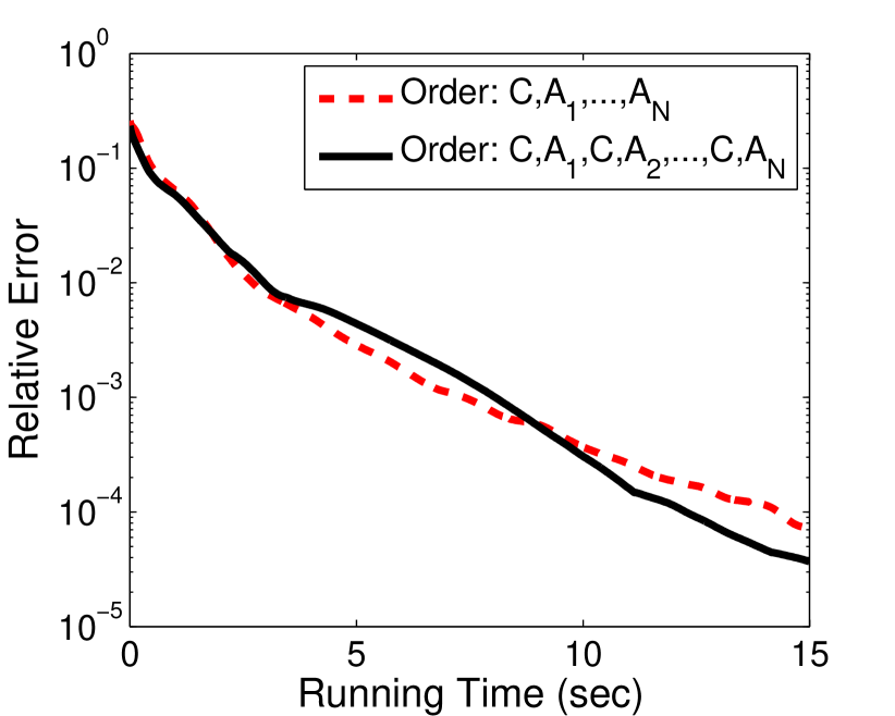
(a) random dataset

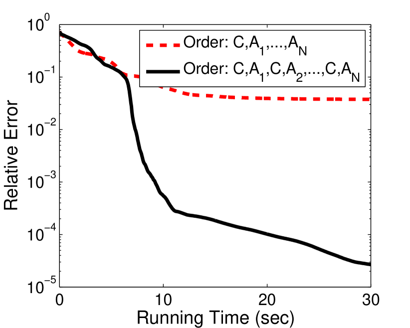
(b) Swimmer dataset

Data: tensor $\boldsymbol{\mathcal{M}}$, core dimension $(R_{1},\cdots,R_{N})$, parameters $\lambda_{c},\lambda_{1},\cdots,\lambda_{N}\geq 0$, and $(\boldsymbol{\mathcal{C}}^{-1},\mathbf{A}^{-1})=(\boldsymbol{\mathcal{C}}^{0},\mathbf{A}^{0})$.

for $k=1,2,\cdots$ do

       Set $\boldsymbol{\mathcal{C}}^{k,-1}=\boldsymbol{\mathcal{C}}^{k,0}=\boldsymbol{\mathcal{C}}^{0}$ if $k=1$ and $\boldsymbol{\mathcal{C}}^{k,-1}=\boldsymbol{\mathcal{C}}^{k-1,N-1},\ \boldsymbol{\mathcal{C}}^{k,0}=\boldsymbol{\mathcal{C}}^{k-1,N}$ otherwise.

       for $n=1,\cdots,N$ do

             Choose $L_{c}^{k,n}$ to be a Lipschitz constant of $\nabla_{\boldsymbol{\mathcal{C}}}\ell(\boldsymbol{\mathcal{C}},\mathbf{A}_{j<n}^{k},\mathbf{A}_{j\geq n}^{k-1})$ about $\boldsymbol{\mathcal{C}}$.

             Choose $\omega_{c}^{k,n}\geq 0$ and set $\hat{\boldsymbol{\mathcal{C}}}^{k,n}={\boldsymbol{\mathcal{C}}}^{k,n-1}+\omega_{c}^{k,n}({\boldsymbol{\mathcal{C}}}^{k,n-1}-{\boldsymbol{\mathcal{C}}}^{k,n-2})$.

             Update $\boldsymbol{\mathcal{C}}$ by

$${\boldsymbol{\mathcal{C}}}^{k,n}=\max\left(0,\hat{\boldsymbol{\mathcal{C}}}^{k,n}-\frac{1}{L_{c}^{k,n}}\nabla_{\boldsymbol{\mathcal{C}}}\ell(\hat{\boldsymbol{\mathcal{C}}}^{k,n},\mathbf{A}_{j<n}^{k},\mathbf{A}_{j\geq n}^{k-1})-\frac{\lambda_{c}}{L_{c}^{k,n}}\right);$$ (13)

Choose $L_{n}^{k}$ to be a Lipschitz constant of $\nabla_{\mathbf{A}_{n}}\ell(\boldsymbol{\mathcal{C}}^{k,n},\mathbf{A}_{j<n}^{k},\mathbf{A}_{n},\mathbf{A}_{j<n}^{k-1})$ about $\mathbf{A}_{n}$.

             Choose $\omega_{n}^{k}\geq 0$ and set $\hat{\mathbf{A}}_{n}^{k}=\mathbf{A}_{n}^{k-1}+\omega_{n}^{k}(\mathbf{A}_{n}^{k-1}-\mathbf{A}_{n}^{k-2})$.

             Update $\mathbf{A}_{n}$ by

$$\mathbf{A}_{n}^{k}=\max\left(0,\hat{\mathbf{A}}_{n}^{k}-\frac{1}{L_{n}^{k}}\nabla_{\mathbf{A}_{n}}\ell(\boldsymbol{\mathcal{C}}^{k,n},\mathbf{A}_{j<n}^{k},\hat{\mathbf{A}}_{n}^{k},\mathbf{A}_{j>n}^{k-1})-\frac{\lambda_{n}}{L_{n}^{k}}\right).$$ (14)

if $F({\boldsymbol{\mathcal{C}}}^{k,n},\mathbf{A}_{j\leq n}^{k},\mathbf{A}_{j>n}^{k-1})>F({\boldsymbol{\mathcal{C}}}^{k,n-1},\mathbf{A}_{j<n}^{k},\mathbf{A}_{j\geq n}^{k-1})$ then

                  ReDo Re-update ${\boldsymbol{\mathcal{C}}}^{k,n}$ and $\mathbf{A}_{n}^{k}$ by (13) and (14) with $\hat{\boldsymbol{\mathcal{C}}}^{k,n}={\boldsymbol{\mathcal{C}}}^{k,n-1}$ and $\hat{\mathbf{A}}_{n}^{k}=\mathbf{A}_{n}^{k-1}$, respectively.

                  

            

       Set $\boldsymbol{\mathcal{C}}^{k}=\boldsymbol{\mathcal{C}}^{k,N}$.

       if Some stopping conditions are satisfied then

             Output $(\boldsymbol{\mathcal{C}}^{k},\mathbf{A}_{1}^{k},\cdots,\mathbf{A}_{N}^{k})$ and stop.

      

Algorithm 1 Alternating proximal gradient for sparse NTD

Remark 2.2.

We do re-update in Line 1 to make the objective nonincreasing. The monotonicity of the objective is important since the algorithm may perform unstably without the re-update. The computational cost of one objective evaluation is much cheaper than, actually not in the same order as, one gradient computation. Detailed complexity analysis is listed in Appendix B. Moreover, in each one of our experiments, the re-update occurs only a few times (often less than 10), so it needs only a little more computations.

If some $\lambda_{n}$ and/or $\lambda_{c}$ vanish, we further do projections

$$\boldsymbol{\mathcal{C}}^{k,n}=\min\left(\max(1,\|\boldsymbol{\mathcal{M}}\|_{\infty}),\boldsymbol{\mathcal{C}}^{k,n}\right)$$ (15)

after (13) and

$$\mathbf{A}_{n}^{k}=\min\left(\max(1,\|\boldsymbol{\mathcal{M}}\|_{\infty}),\mathbf{A}_{n}^{k}\right)$$ (16)

after (14). Omitting the superscript, it is easy to show that (15) and (16) respectively solve (8) and (10) with the extra constraints (7) and (6).

2.3 Parameter settings

In our implementation of Algorithm 1, we set

$$L_{c}^{k,n}=\max\big{(}1,\left\|(\mathbf{A}_{N}^{k-1})^{\top}\mathbf{A}_{N}^{k-1}\otimes\cdots\otimes(\mathbf{A}_{n}^{k-1})^{\top}\mathbf{A}_{n}^{k-1}\otimes(\mathbf{A}_{n-1}^{k})^{\top}\mathbf{A}_{n-1}^{k}\otimes\cdots\otimes(\mathbf{A}_{1}^{k})^{\top}\mathbf{A}_{1}^{k}\right\|\big{)},$$

where $\|\cdot\|$ denotes matrix operator norm. Note that computing $L_{c}^{k,n}$ does not need to form the expensive Kronecker product because

$$\left\|\mathbf{A}_{N}^{\top}\mathbf{A}_{N}\otimes\cdots\otimes\mathbf{A}_{1}^{\top}\mathbf{A}_{1}\right\|=\prod_{i=1}^{N}\left\|\mathbf{A}_{i}^{\top}\mathbf{A}_{i}\right\|.$$

In the same way, we set

$$L_{n}^{k}=\max\big{(}1,\|\mathbf{B}_{n}^{k}(\mathbf{B}_{n}^{k})^{\top}\|\big{)},$$ (17)

where

$$\mathbf{B}_{n}^{k}=\mathbf{C}_{(n)}^{k,n}\left(\mathbf{A}_{N}^{k-1}\otimes\cdots\otimes\mathbf{A}_{n+1}^{k-1}\otimes\mathbf{A}_{n-1}^{k}\otimes\cdots\otimes\mathbf{A}_{1}^{k}\right)^{\top}.$$ (18)

In addition, we take

$$\omega_{c}^{k,n}=\min\left(\hat{\omega}_{c}^{k,n},0.9999\sqrt{\frac{L_{c}^{k,n-1}}{L_{c}^{k,n}}}\right),$$ (19)

where $\hat{\omega}_{c}^{k,n}$ follows

$$\hat{\omega}_{c}^{k,n}=\frac{t^{k,n-1}-1}{t^{k,n}},$$ (20a)

$$t^{1,0}_{c}=1,\ t^{k,0}_{c}=t^{k-1,N}_{c},\text{ for }k\geq 2,$$ (20b)

$$t^{k,n}_{c}=\frac{1}{2}\left(1+\sqrt{1+4(t^{k,n-1}_{c})^{2}}\right),\text{ for }k\geq 1,n=1,\cdots,N.$$ (20c)

In the same way,

$$\omega_{n}^{k}=\min\left(\hat{\omega}^{k},0.9999\sqrt{\frac{L_{n}^{k-1}}{L_{n}^{k}}}\right),$$ (21)

where $\hat{\omega}^{k}$ follows

$$\hat{\omega}^{k}=\frac{t^{k-1}-1}{t^{k}},$$ (22a)

$$t^{0}=1,\ t^{k}=\frac{1}{2}\left(1+\sqrt{1+4(t^{k-1})^{2}}\right),\text{ for }k\geq 1.$$ (22b)

Remark 2.3.

We perform “min” operation in (19) and (21) for convergence; see Theorem 2. The weights $\hat{\omega}_{c}^{k,n}$ in (20) and $\hat{\omega}^{k}$ in (22) are the same as that used in [3] for convex problems. Numerically, we observe that the extrapolation technique using the weights given in (19) and (21) can significantly speed up our algorithm. We also tested APG with the dynamically updated weight used in [34, 23] for non-convex matrix completion problem and observed that APG performs as well as that with the above extrapolation weights.

2.4 Per-iteration complexity

Suppose $\boldsymbol{\mathcal{M}}\in\mathbb{R}^{I_{1}\times\ldots\times I_{N}}$ and the core tensor $\boldsymbol{\mathcal{C}}\in\mathbb{R}^{R_{1}\times\ldots\times R_{N}}$. Then the per-iteration cost of Algorithm 1 is roughly

$$N\cdot\mathcal{O}\left(\sum_{j=1}^{N}\big{(}\prod_{i=1}^{j}R_{i}\big{)}\big{(}\prod_{i=j}^{N}I_{i}\big{)}+\sum_{j=1}^{N}\big{(}\prod_{i=1}^{j}I_{i}\big{)}\big{(}\prod_{i=j}^{N}R_{i}\big{)}\right).$$ (23)

The detailed analysis is given in Appendix B.

Remark 2.4.

If $N=\mathcal{O}(1)$ and $\max_{n}R_{n}\leq\mathcal{O}(\log\prod_{i=1}^{N}I_{i})$, then the per-iteration cost of Algorithm 1 is scalable about the data size $\prod_{i=1}^{N}I_{i}$.

2.5 Convergence results

It is shown in [35] that the APG method with cyclic block updating rule has global convergence to a stationary point. Since Algorithm 1 uses a different block updating order, its convergence cannot be directly obtained from [35]. However, we can still obtain the global convergence, which is summarized in Theorem 2. Although the proof idea for Theorem 2 is similar to that in [35], some places need careful modifications. Hence, for completeness, we include a modified proof in the Appendix.

Theorem 2.

Let $\big{\{}\boldsymbol{\mathcal{W}}^{k}\triangleq(\boldsymbol{\mathcal{C}}^{k},\mathbf{A}^{k})\big{\}}$ be the sequence generated by Algorithm 1. If $\lambda_{c},\lambda_{1},\cdots,\lambda_{N}$ are all positive, and

1. There exist positive constants $L_{d},L_{u}$ such that $L_{c}^{k,n},L_{n}^{k}\in[L_{d},L_{u}]$;

2. There is a positive constant $\delta_{\omega}<1$ such that $\omega_{c}^{k,n}\leq\delta_{\omega}\sqrt{\frac{L_{c}^{k,n-1}}{L_{c}^{k,n}}}$ and $\omega_{n}^{k}\leq\delta_{\omega}\sqrt{\frac{L_{n}^{k-1}}{L_{n}^{k}}}$ for all $n$ and $k$, where we use the notation $L_{c}^{k,0}=L_{c}^{k-1,N}$;

then $\boldsymbol{\mathcal{W}}^{k}$ converges to a stationary point $\bar{\boldsymbol{\mathcal{W}}}$ of (5).

Remark 2.5.

Positivity of sparse parameters implies the boundedness of $\{\boldsymbol{\mathcal{W}}^{k}\}$, and thus the existence of $L_{d}$ and $L_{u}$ can be guaranteed if $L_{c}^{k,n}$ and $L_{n}^{k}$ are taken as in section 2.3.

3 Sparse nonnegative Tucker decomposition with missing values

For some applications, $\boldsymbol{\mathcal{M}}$ may not be fully observed. This section modifies Algorithm 1 to handle this case. The problem is formulated as

$$\begin{array}[]{l}\underset{\boldsymbol{\mathcal{C}},\mathbf{A}}{\min}\ F_{\Omega}(\boldsymbol{\mathcal{C}},\mathbf{A})\equiv\frac{1}{2}\|\mathcal{P}_{\Omega}(\boldsymbol{\mathcal{C}}\times_{1}\mathbf{A}_{1}\cdots\times_{N}\mathbf{A}_{N}-\boldsymbol{\mathcal{M}})\|_{F}^{2}+\lambda_{c}\|\boldsymbol{\mathcal{C}}\|_{1}+\overset{N}{\underset{n=1}{\sum}}\lambda_{n}\|\mathbf{A}_{n}\|_{1},\\[5.69046pt] \text{ s.t. }\boldsymbol{\mathcal{C}}\in\mathbb{R}^{R_{1}\times\cdots\times R_{N}}_{+},\mathbf{A}_{n}\in\mathbb{R}^{I_{n}\times R_{n}}_{+},~{}n=1,\cdots,N,\end{array}$$ (24)

where $\Omega$ indexes the observed entries of $\boldsymbol{\mathcal{M}}$, and $\mathcal{P}_{\Omega}(\boldsymbol{\mathcal{A}})$ keeps the entries of $\boldsymbol{\mathcal{A}}$ in $\Omega$ and zeros out all others. As did in [34, 36], we introduce variable $\boldsymbol{\mathcal{X}}$, restrict $\mathcal{P}_{\Omega}(\boldsymbol{\mathcal{X}})=\mathcal{P}_{\Omega}(\boldsymbol{\mathcal{M}})$, and write (24) equivalently to

$$\begin{array}[]{cl}\underset{\boldsymbol{\mathcal{C}},\mathbf{A},\boldsymbol{\mathcal{X}}}{\min}&\frac{1}{2}\|\boldsymbol{\mathcal{C}}\times_{1}\mathbf{A}_{1}\cdots\times_{N}\mathbf{A}_{N}-\boldsymbol{\mathcal{X}}\|_{F}^{2}+\lambda_{c}\|\boldsymbol{\mathcal{C}}\|_{1}+\overset{N}{\underset{n=1}{\sum}}\lambda_{n}\|\mathbf{A}_{n}\|_{1},\\[5.69046pt] \text{ s.t. }&\boldsymbol{\mathcal{C}}\in\mathbb{R}^{R_{1}\times\cdots\times R_{N}}_{+},\mathbf{A}_{n}\in\mathbb{R}^{I_{n}\times R_{n}}_{+},~{}n=1,\cdots,N,~{}\mathcal{P}_{\Omega}(\boldsymbol{\mathcal{X}})=\mathcal{P}_{\Omega}(\boldsymbol{\mathcal{M}}).\end{array}$$ (25)

To modify Algorithm 1 for (24) or equivalently (25), we set $\boldsymbol{\mathcal{X}}^{0}=\mathcal{P}_{\Omega}(\boldsymbol{\mathcal{M}})$ in the beginning. At the $k$-th iteration of Algorithm 1, we use $\boldsymbol{\mathcal{M}}=\boldsymbol{\mathcal{X}}^{k-1}$, wherever $\boldsymbol{\mathcal{M}}$ is referred to. After Line 1 of Algorithm 1, update $\boldsymbol{\mathcal{X}}$ by

$$\boldsymbol{\mathcal{X}}^{k}=\mathcal{P}_{\Omega}(\boldsymbol{\mathcal{M}})+\mathcal{P}_{\Omega^{c}}(\boldsymbol{\mathcal{C}}^{k}\times_{1}\mathbf{A}_{1}^{k}\cdots\times_{N}\mathbf{A}_{N}^{k}).$$ (26)

Compared to Algorithm 1, the modified method needs extra computation for the update (26), which costs about $2\sum_{j=1}^{N}\big{(}\prod_{i=1}^{j}I_{i}\big{)}\big{(}\prod_{i=j}^{N}R_{i}\big{)}.$ Therefore, the per-iteration complexity of the modified algorithm is still scalable about the data size if $N=\mathcal{O}(1)$ and $\max_{n}R_{n}\leq\mathcal{O}(\log\prod_{i=1}^{N}I_{i})$. In addition, following the proof of Theorem 2, one can show that the same convergence result holds for the modified algorithm.

4 Extensions

For some applications, the core tensor $\boldsymbol{\mathcal{C}}$ may not be required nonnegative [10]. Algorithm 1 can be modified to handle this case by changing (13) to

$${\boldsymbol{\mathcal{C}}}^{k,n}=\mathcal{S}_{\frac{\lambda_{c}}{L_{c}^{k,n}}}\left(\hat{\boldsymbol{\mathcal{C}}}^{k,n}-\frac{1}{L_{c}^{k,n}}\nabla_{\boldsymbol{\mathcal{C}}}\ell(\hat{\boldsymbol{\mathcal{C}}}^{k,n},\mathbf{A}_{j<n}^{k},\mathbf{A}_{j\geq n}^{k-1})\right),$$ (27)

where $\mathcal{S}_{\mu}(\boldsymbol{\mathcal{X}})$ is a soft-thresholding operator defined component-wisely as

$$\mathcal{S}_{\mu}(x)={\mathrm{sign}}(x)\cdot\max(0,|x|-\mu).$$

The APG method can also be adapted to solve sparse higher-order principal component analysis (HOPCA), which imposes orthogonality constraint on each factor matrix. The problem is formulated as

$$\begin{array}[]{l}\underset{\boldsymbol{\mathcal{C}},\mathbf{A}}{\min}~{}\frac{1}{2}\|\boldsymbol{\mathcal{C}}\times_{1}\mathbf{A}_{1}\cdots\times_{N}\mathbf{A}_{N}-\boldsymbol{\mathcal{M}}\|_{F}^{2}+\lambda_{c}\|\boldsymbol{\mathcal{C}}\|_{1}+\overset{N}{\underset{n=1}{\sum}}\lambda_{n}\|\mathbf{A}_{n}\|_{1},\\ \text{ s.t. }\mathbf{A}_{n}^{\top}\mathbf{A}_{n}=\mathbf{I}_{n},~{}n=1,\cdots,N,\end{array}$$ (28)

where $\mathbf{I}_{n}$ is an identity matrix of appropriate size. When $\lambda_{c}=0$, the optimal $\boldsymbol{\mathcal{C}}=\boldsymbol{\mathcal{M}}\times_{1}\mathbf{A}_{1}^{\top}\cdots\times_{N}\mathbf{A}_{N}$, and one can eliminate $\boldsymbol{\mathcal{C}}$ as shown in [19]. The concurrency of sparsity and orthogonality constraints makes the problem much more difficult. The work [1] considers rank-1 factor matrix with only one column and relaxes the orthogonality constraint to $\mathbf{A}_{n}^{\top}\mathbf{A}_{n}\leq 1$. Then it applies block coordinate minimization method to solve the relaxed problem. When some $\mathbf{A}_{n}$ has more than one columns, we relax (28) to

$$\begin{array}[]{l}\underset{\boldsymbol{\mathcal{C}},\mathbf{A}}{\min}~{}\frac{1}{2}\|\boldsymbol{\mathcal{C}}\times_{1}\mathbf{A}_{1}\cdots\times_{N}\mathbf{A}_{N}-\boldsymbol{\mathcal{M}}\|_{F}^{2}+\lambda_{c}\|\boldsymbol{\mathcal{C}}\|_{1}+\overset{N}{\underset{n=1}{\sum}}\lambda_{n}\|\mathbf{A}_{n}\|_{1}+\frac{\mu}{2}\overset{N}{\underset{n=1}{\sum}}\underset{i\neq j}{\sum}\left({\bf a}_{n,i}^{\top}{\bf a}_{n,j}\right)^{2}\\ \text{ s.t. }\|{\bf a}_{n,j}\|_{2}\leq 1,~{}n=1,\cdots,N,\forall j,\end{array}$$ (29)

where ${\bf a}_{n,j}$ denotes the $j$-th column of $\mathbf{A}_{n}$, $\sum_{i\neq j}\left({\bf a}_{n,i}^{\top}{\bf a}_{n,j}\right)^{2}$ is used to promote the orthogonality of $\mathbf{A}_{n}$, and $\mu$ is a penalty parameter. We want to mention that our orthogonality regularization term is similar to that used in [30] for promoting the discrepancy of dictionaries and also that used on pp. 222 of [7].

Our method for (29) is similar to Algorithm 1 and cycles over the variables by $\boldsymbol{\mathcal{C}},\mathbf{A}_{1},\boldsymbol{\mathcal{C}},\mathbf{A}_{2},\cdots,\boldsymbol{\mathcal{C}},\mathbf{A}_{N}$. The update of $\boldsymbol{\mathcal{C}}$ is done by (27), and $\mathbf{A}_{n}$ is updated one column by one column. Specifically, assume the current iterate is $(\boldsymbol{\mathcal{C}}^{k,n},\mathbf{A}_{i<n}^{k},\mathbf{A}_{i\geq n}^{k-1})$. Let $\mathbf{B}_{n}^{k}$ be the one obtained from (18). Using (37), we update the columns of $\mathbf{A}_{n}$ from $j=1$ to $R_{n}$ by

$${\bf a}_{n,j}^{k}=\operatorname*{argmin}_{\|{\bf a}_{n,j}\|_{2}\leq 1} ~{}\frac{1}{2}\big{\|}{\bf a}_{n,j}{\bf b}_{n}^{k,j}+(\tilde{\mathbf{A}}_{n}^{k})_{j^{c}}(\mathbf{B}_{n}^{k})^{j^{c}}-\mathbf{M}_{(n)}\big{\|}_{F}^{2}+\lambda_{n}\|{\bf a}_{n,j}\|_{1}$$ (30)

$$+\mu\left(\big{\langle}(\tilde{\mathbf{A}}_{n}^{k})_{j^{c}}(\tilde{\mathbf{A}}_{n}^{k})_{j^{c}}^{\top}\hat{{\bf a}}_{n,j}^{k},{\bf a}_{n,j}-\hat{{\bf a}}_{n,j}^{k}\big{\rangle}+\frac{L_{n,j}^{k}}{2}\|{\bf a}_{n,j}-\hat{{\bf a}}_{n,j}^{k}\|_{2}^{2}\right),$$

where ${\bf b}_{n}^{k,j}$ denotes the $j$-th row of $\mathbf{B}_{n}^{k}$, $(\mathbf{B}_{n}^{k})^{j^{c}}$ is the submatrix by taking all rows of $\mathbf{B}_{n}^{k}$ except the $j$-th one,

$$\hat{{\bf a}}_{n,j}^{k}={{\bf a}}_{n,j}^{k-1}+\omega_{n,j}^{k}({{\bf a}}_{n,j}^{k-1}-{{\bf a}}_{n,j}^{k-2})$$

is an extrapolated point, $(\tilde{\mathbf{A}}_{n}^{k})_{j^{c}}$ is short for $\big{(}{\bf a}_{n,1}^{k},\cdots,{\bf a}_{n,j-1}^{k},{\bf a}_{n,j+1}^{k-1},\cdots,{\bf a}_{n,R_{n}}^{k-1}\big{)}$, and $L_{n,j}^{k}$ is a Lipschitz constant of the gradient of

$$\frac{1}{2}\left(\sum_{i<j}\big{(}{\bf a}_{n,j}^{\top}{\bf a}_{n,i}^{k}\big{)}^{2}+\sum_{i>j}\big{(}{\bf a}_{n,j}^{\top}{\bf a}_{n,i}^{k-1}\big{)}^{2}\right)$$

with respect to ${\bf a}_{n,j}$. One can easily write the update in (30) explicitly as

$${\bf a}_{n,j}^{k}=\mathcal{P}_{B_{1}}\left[\mathcal{S}_{\frac{\lambda_{n}}{b+\mu L}}\left(\frac{\mu L}{b+\mu L}\hat{{\bf a}}_{n,j}^{k}-\frac{\big{(}(\tilde{\mathbf{A}}_{n}^{k})_{j^{c}}(\mathbf{B}_{n}^{k})^{j^{c}}-\mathbf{M}_{(n)}\big{)}\big{(}{\bf b}_{n}^{k,j}\big{)}^{\top}}{b+\mu L}-\frac{\mu}{b+\mu L}(\tilde{\mathbf{A}}_{n}^{k})_{j^{c}}(\tilde{\mathbf{A}}_{n}^{k})_{j^{c}}^{\top}\hat{{\bf a}}_{n,j}^{k}\right)\right],$$ (31)

where $b=\|{\bf b}_{n}^{k,j}\|_{2}^{2}$, $L=L_{n,j}^{k}$, and $\mathcal{P}_{B_{1}}$ denotes the projection to unit Euclidean ball.

Following the proof of Theorem 2, one can show that the method described above has global convergence if the parameters $L_{n,j}^{k}$, $\omega_{n,j}^{k},L_{c}^{k,n},\omega_{c}^{k,n}$ satisfy conditions as those in Theorem 2. We do not repeat it here.

5 Numerical experiments

In this section, we compare Algorithm 1 (APG), HONMF in [26], and HALS in [28] for solving (sparse) NTD on both synthetic and real world data. Also, we test the modified version of Algorithm 1 and HONMF for solving (sparse) NTD with missing values. The code of all compared solvers is accessible online. There are of course more other solvers for (sparse) NTD such as dGN in [29], ALS in [12], and CCD in [24]. However, we do not get the code of dGN, and the code of CCD and ALS only handles the case where the core tensor is fixed to identity tensor.

All the tests are performed on a laptop with an i7-620m CPU and 3GB RAM and running 32-bit Windows 7 and MATLAB 2010b with Statistics Toolbox and Tensor Toolbox of version 2.5 [2].

5.1 Implementation details

This subsection specifies the implementation of Algorithm 1 in details about initialization and stopping criteria. Unless specified, all parameters for HONMF and HALS are set to their default values.

Initialization

For all the compared algorithms, we use the same starting point. Throughout the tests, we first randomly generate ${\mathbf{A}}_{1}^{0},\cdots,{\mathbf{A}}_{N}^{0}$ and then process them by the Higher-order Orthogonal Iteration algorithm in [9]. Specifically, for (5), let

$$\boldsymbol{\mathcal{B}}=\boldsymbol{\mathcal{M}}\times_{1}(\mathbf{A}_{1}^{0})^{\top}\cdots\times_{n-1}(\mathbf{A}_{n-1}^{0})^{\top}\times_{n+1}(\mathbf{A}_{n+1}^{0})^{\top}\times_{N}(\mathbf{A}_{N}^{0})^{\top},$$ (32)

and update $\mathbf{A}_{n}^{0}=\max(\epsilon_{machine},\mathbf{U}_{n})$ alternatively for $n=1,\cdots,N$, where $\epsilon_{machine}$ stands for machine precision and $\mathbf{U}_{n}$ contains the left $R_{n}$ singular vectors of $\mathbf{B}_{(n)}$. Then set

$$\boldsymbol{\mathcal{C}}^{0}=\boldsymbol{\mathcal{M}}\times_{1}(\mathbf{A}_{1}^{0})^{\top}\cdots\times_{N}(\mathbf{A}_{N}^{0})^{\top}.$$ (33)

For (24), we use the same initialization except replacing $\boldsymbol{\mathcal{M}}$ to $\mathcal{P}_{\Omega}(\boldsymbol{\mathcal{M}})$ in (32) and (33). It is observed that all the algorithms perform better with this kind of starting point than a random one, in both convergence speed and chance of avoiding local minima. The use of strictly positive initial points is mainly due to the consideration that HONMF does not allow its iterates to have zero components.

Stopping criteria

We stop Algorithm 1 and its modified version in section 3 if a maximum number of iterations or maximum time is reached or one of the following conditions is satisfied

$$\frac{\|\mathcal{P}_{\Omega}\big{(}\boldsymbol{\mathcal{C}}^{k}\times_{1}\mathbf{A}_{1}^{k}\cdots\times_{N}\mathbf{A}_{N}^{k}-\boldsymbol{\mathcal{M}}\big{)}\|_{F}}{\|\mathcal{P}_{\Omega}(\boldsymbol{\mathcal{M}})\|_{F}}\leq tol,\ \text{ for some }k,$$ (34a)

$$\frac{|F_{\Omega}^{k}-F_{\Omega}^{k+1}|}{1+F_{\Omega}^{k}}\leq tol,\ \text{ for three consecutive }k\text{'s},$$ (34b)

where $F_{\Omega}^{k}\triangleq F_{\Omega}(\boldsymbol{\mathcal{C}}^{k},\mathbf{A}_{1}^{k},\cdots,\mathbf{A}_{N}^{k})$ and $tol$ is a small positive value specified below. Note that for Algorithm 1, $\Omega$ contains all indices.

5.2 Nonnegative Tucker decomposition

In this subsection, we compare APG, HONMF, and HALS on solving NTD, i.e., (5) with all of $\lambda_{c},\lambda_{1},\cdots,\lambda_{N}$ set to zero. We first test them on two sets of synthetic data and then on two image datasets.

Synthetic data

In the first synthetic dataset, each tensor has the form $\boldsymbol{\mathcal{M}}=\boldsymbol{\mathcal{C}}\times_{1}\mathbf{A}_{1}\times_{2}\mathbf{A}_{2}\times_{3}\mathbf{A}_{3}$, where $\boldsymbol{\mathcal{C}}$ is generated by MATLAB’s command rand(5,5,5) and each $\mathbf{A}_{i}$ by command max(0,randn(80,5)). Then $\boldsymbol{\mathcal{M}}$ is re-scaled to have unit maximum component. Each tensor $\boldsymbol{\mathcal{M}}$ in the second test is generated in the same way but has an unbalanced dimension $10\times 10\times 1000$, and the core tensor is $3\times 3\times 30$. We emphasize that uniformly random $\boldsymbol{\mathcal{C}}$ makes the problem more difficult than Gaussian random one because the former is not zero-mean. The true dimension is used in our tests, namely, $I_{n}=50,R_{n}=5,\forall n$ is set in (5) for the first dataset and $(I_{1},I_{2},I_{3})=(10,10,1000),(R_{1},R_{2},R_{3})=(3,3,30)$ for the second one.

We add normalized noise to each tensor, namely, we input to each algorithm with $\boldsymbol{\mathcal{M}}^{nois}=\boldsymbol{\mathcal{M}}+\eta\frac{\|\boldsymbol{\mathcal{M}}\|_{F}}{\|\boldsymbol{\mathcal{N}}\|_{F}}\boldsymbol{\mathcal{N}}$, where the entries of $\boldsymbol{\mathcal{N}}$ follow i.i.d standard Gaussian distribution. We run each algorithm to $t_{\max}$ (sec) and compare their relative error $\frac{\|\boldsymbol{\mathcal{C}^{r}}\times_{1}\mathbf{A}_{1}^{r}\times_{2}\mathbf{A}_{2}^{r}\times_{3}\mathbf{A}_{3}^{r}-\boldsymbol{\mathcal{M}}\|_{F}}{\|\boldsymbol{\mathcal{M}}\|_{F}}$, where $(\boldsymbol{\mathcal{C}}^{r},\mathbf{A}_{1}^{r},\mathbf{A}_{2}^{r},\mathbf{A}_{3}^{r})$ is a solution obtained by running an algorithm. Table 1 shows the average relative error and number of iterations for the three algorithms over 20 independent runs with $t_{\max}=10$ and different $\eta$’s. Figure 2 plots how the relative error changes with respect to the running time for each algorithm with $t_{\max}=20$ and also to iterations.

From the table, we see that APG performs significantly better than HONMF and HALS for noiseless case. When there is noise, i.e., $\eta>0$, APG is still much better than HONMF and comparable to HALS. From the figure, we see that HONMF converges very slowly in both cases and HALS works well for $\boldsymbol{\mathcal{M}}$ with balanced dimension but converges slowly for the unbalanced one. APG converges faster than both HONMF and HALS, in particular for the unbalanced case.

To see how the algorithms perform on decomposing nonnegative tensors with larger ranks, we also test them on random tensors generated in the same way as above with size $80\times 80\times 80$ and each mode rank $r$, where $r$ varies from 3 to 30 with increment 3. Each algorithm runs to 1,000 iterations. Figure 3 plots the average relative errors of 10 independent runs for each algorithm. From the figure, we see that APG performs consistently better than HONMF and HALS and much better when $r$ is small.

Table 1: Average results over 20 independent runs by APG, HONMF and HALS on two synthetic datasets

	APG		HONMF		HALS
noise level	rel. err.	# iter	rel. err.	# iter	rel. err.	# iter
$(I_{1},I_{2},I_{3})=(80,80,80),(R_{1},R_{2},R_{3})=(5,5,5)$
$\eta=0.00$	7.09e-004	467	6.06e-002	87	2.45e-003	758
$\eta=0.05$	2.79e-003	468	6.86e-002	48	3.27e-003	732
$\eta=0.10$	4.78e-003	466	7.15e-002	47	5.44e-003	759
$(I_{1},I_{2},I_{3})=(10,10,1000),(R_{1},R_{2},R_{3})=(3,3,30)$
$\eta=0.00$	5.12e-004	653	2.52e-002	287	2.97e-003	737
$\eta=0.05$	1.49e-002	668	3.00e-002	232	1.50e-002	739
$\eta=0.10$	3.02e-002	670	3.84e-002	222	3.01e-002	740

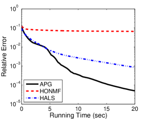
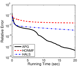
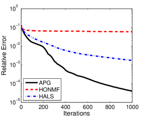
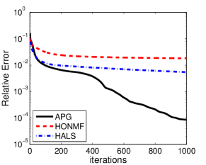
Fig. 2: Convergence behavior of APG, HONMF and HALS on synthetic data. Left: $80\times 80\times 80$ nonnegative tensor $\boldsymbol{\mathcal{M}}$ and $5\times 5\times 5$ core tensor $\boldsymbol{\mathcal{C}}$; Right: $10\times 10\times 1000$ nonnegative tensor $\boldsymbol{\mathcal{M}}$ and $3\times 3\times 30$ core tensor $\boldsymbol{\mathcal{C}}$.

Image data

The first test uses the Swimmer dataset constructed in [11], which has 256 swimmer images and each one has resolution of $32\times 32$. We form a $32\times 32\times 256$ tensor $\boldsymbol{\mathcal{M}}$ using the dataset and then re-scale it to have unit maximum component. The core dimension is set to $(24,20,20)$. We run APG, HONMF, and HALS to $t_{\max}=30$ (sec) and plot their relative errors on the left of Figure 4. The second test uses a brain MRI image of size $181\times 217\times 181$, which has been tested in [24] for sparse nonnegative tensor decomposition. We re-scale it to have unit maximum pixel and set the core size to $(30,30,30)$. All the three algorithms run to $t_{\max}=600$ (sec), and the relative errors are plotted on the right of Figure 4. From the figure, we see that HONMF performs the worst and HALS decreases the objective faster than APG in the beginning but APG eventually converges faster. In particular for the test with Swimmer dataset, the overall convergence speed of APG is much faster than that of HALS, and APG reaches much lower relative errors while HALS seems to be trapped at some local solution.

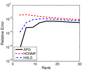
Fig. 3: Average relative errors of 10 independent runs for APG, HONMF, and HALS on synthetic tensors of size $80\times 80\times 80$ and with each mode rank $r$.

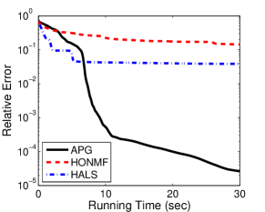
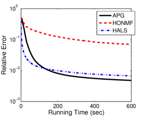
Fig. 4: Convergence behavior of APG, HONMF, and HALS on Swimmer dataset (left) and a brain MRI image (right).

5.3 Sparse nonnegative Tucker decomposition

In this subsection, we compare APG and HONMF for solving sparse NTD, i.e., (5) with at least one of $\lambda_{c},\lambda_{1},\cdots,\lambda_{N}$ set to be positive. HALS is not coded for sparse NTD. Hence, we do not include HALS for comparison.

We compare APG and HONMF on the brain MRI image used above and the CBCL face image dataset which has been tested in [32] for nonnegative tensor decomposition. For the brain MRI image, we set $R_{1}=R_{2}=R_{3}=30$ and $\lambda_{c}=\lambda_{1}=\lambda_{2}=\lambda_{3}=0.5$ in (5). We run APG and HONMF to $t_{\max}=300$ (sec) and report the results at time $t=100,200,300$ (sec). Table 2 summarizes the average results of 10 independent runs. The “core den.” is calculated by $\frac{\#\text{ nonzeros of }\boldsymbol{\mathcal{C}}^{r}}{30^{3}}$ and “fac. den.” by $\frac{\sum_{n=1}^{3}\#\text{ nonzeros of }\mathbf{A}_{n}^{r}}{30\cdot(181+217+181)}$. We see that APG reaches much lower objective values and relative errors than those by HONMF. In addition, the solutions obtained by APG are sparser than those by HONMF and are potentially easier to interpret.

The CBCL dataset has 6977 face images, and each one is $19\times 19$. We use all these images to form a $19\times 19\times 6977$ nonnegative tensor $\boldsymbol{\mathcal{M}}$, which is then re-scaled to have unit maximum component. The core size is set to $(R_{1},R_{2},R_{3})=(5,5,50)$ and the sparsity parameters to $\lambda_{c}=0.5,\lambda_{1}=\lambda_{2}=\lambda_{3}=0$, namely, we only want the core tensor to be sparse. Table 3 reports the average results obtained by APG and HONMF at running time $t=25,50,75,100$ (sec). We see that APG reaches much lower objective values and also lower relative errors than those by HONMF. The solutions given by APG are much sparser than those by HONMF. This may be because APG uses the constraints (6) while HONMF simply normalizes each factor matrix after every iteration. However, it somehow validates the use of the constraints (6).

Table 2: Average results by APG and HONMF on a brain MRI image with the core size $R_{1}=R_{2}=R_{3}=30$

	APG					HONMF
time	obj.	rel. err.	fac. den.	core den.	# iter	obj.	rel. err.	fac. den.	core den.	# iter
100	1.6622e+3	6.15e-2	32.45%	7.62%	185	6.2934e+3	1.77e-1	32.47%	31.84%	31
200	8.4659e+2	2.94e-2	23.22%	14.45%	370	4.7762e+3	1.48e-1	30.61%	31.01%	48
300	6.8898e+2	2.25e-2	20.49%	16.87%	555	4.0240e+3	1.30e-1	29.14%	29.91%	63

Table 3: Average results by APG and HONMF on CBCL dataset with the core size $(R_{1},R_{2},R_{3})=(5,5,50)$

	APG				HONMF
time	obj.	rel. err.	core den.	# iter	obj.	rel. err.	core den.	# iter
25	3.2469e+4	2.72e-1	11.45%	135	5.9824e+4	3.63e-1	90.19%	29
50	3.1453e+4	2.68e-1	7.56%	271	5.3017e+4	3.40e-1	69.26%	57
75	3.1370e+4	2.68e-1	6.78%	408	4.9786e+4	3.28e-1	58.03%	84
100	3.1344e+4	2.67e-1	6.46%	545	4.7289e+4	3.20e-1	51.26%	112

5.4 Sparse nonnegative Tucker decomposition with missing values

In this subsection, we test APG for solving (24) on synthetic data and compare it to HONMF on the brain MRI image used above.

Performance of APG with different sample ratios

First, we show that APG using partial observations can achieve similar accuracies as that using full observations. Each tensor has the form $\boldsymbol{\mathcal{M}}=\boldsymbol{\mathcal{C}}\times_{1}\mathbf{A}_{1}\times_{2}\mathbf{A}_{2}\times_{3}\mathbf{A}_{3}$ and is re-scaled to have unit maximum component, where $\boldsymbol{\mathcal{C}}$ is generated by MATLAB’s command max(0,randn(R,R,R)) and each factor matrix $\mathbf{A}_{n}$ by max(0,randn(50,R)) with R varying among $\{5,8,11,14,17,20,23,26\}$. We choose $\text{SR}=10\%,30\%,50\%,100\%$ samples uniformly at random and compare the performance of APG using different SRs. The maximum number of iterations is set to 5,000 and the stopping tolerance to $tol=10^{-5}$. Figure 5 plots the average relative errors and running time (sec) of APG over 20 independent trials. We see that APG using 30% and 50% samples gives similar accuracies as that using full observations. APG with 10% samples can still make relative errors low to about 1% as $R\leq 14$, but $10\%$ samples seem not enough when $R\geq 17$. Longer time by APG with partial observations is due to the extra update (26) and more iterations. When $R\geq 17$, the running time of APG with 10% samples decreases because it stops earlier.

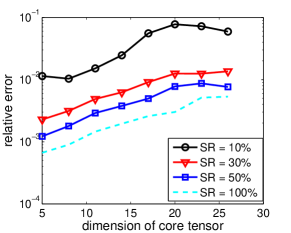
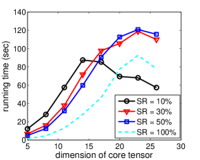
Fig. 5: Average relative errors (left) and runnting time (right) by APG using different sample ratios

Comparison with HONMF

Secondly, we compare APG to HONMF on the brain MRI image used above. The core dimension is set to $R_{1}=R_{2}=R_{3}=30$ and sparsity parameters to $\lambda_{c}=\lambda_{1}=\lambda_{2}=\lambda_{3}=0.5$. We compare the two algorithms using $\text{SR}=10\%,30\%,50\%$ uniformly randomly chosen samples and run them to $t_{\max}=600$ (sec). Table 4 shows the average results at time $t=150,300,450,600$ for different SRs over 5 independent trials. From the table, we see that HONMF fails with 10% samples while APG can still work reasonably. In all cases, APG performs better than HONMF in both accuracy and speed. The solutions given by APG are sparser than those by HONMF for $\text{SR}=30\%,50\%$.

Table 4: Average results by APG and HONMF on a brain MRI image from different samples

	APG					HONMF
time	obj.	rel. err.	fac. den.	core den.	# iter	obj.	rel. err.	fac. den.	core den.	# iter
SR = 10%
150	1.3418e+3	2.32e-1	30.49%	0.72%	208	1.5608e+4	1.00e+0	0.00%	0.00%	67
300	9.3130e+2	1.80e-1	17.03%	0.88%	416	1.5608e+4	1.00e+0	0.00%	0.00%	150
450	7.9761e+2	1.60e-1	14.28%	1.23%	623	1.5608e+4	1.00e+0	0.00%	0.00%	232
600	7.4748e+2	1.53e-1	13.60%	1.40%	831	1.5608e+4	1.00e+0	0.00%	0.00%	315
SR = 30%
150	1.5808e+3	1.27e-1	35.15%	2.31%	191	2.4525e+3	1.88e-1	31.80%	41.87%	40
300	9.0284e+2	8.17e-2	19.65%	4.38%	384	1.9277e+3	1.58e-1	28.90%	38.48%	67
450	7.0151e+2	6.25e-2	17.29%	6.34%	576	1.6362e+3	1.38e-1	26.44%	33.07%	96
600	6.2076e+2	5.34e-2	15.69%	7.60%	769	1.4587e+3	1.25e-1	24.54%	30.12%	129
SR = 50%
150	1.8767e+3	1.08e-1	35.03%	3.64%	184	3.7494e+3	1.91e-1	31.75%	36.66%	40
300	9.5363e+2	5.88e-2	22.42%	7.55%	367	2.8367e+3	1.59e-1	28.70%	40.15%	64
450	7.0877e+2	4.03e-2	19.29%	10.74%	550	2.3369e+3	1.37e-1	26.48%	42.33%	92
600	6.2737e+2	3.32e-2	17.75%	12.41%	733	2.0265e+3	1.23e-1	24.96%	42.58%	124

5.5 Sparse higher-order principal component analysis

We use a simple test with synthetic data to show that (29) can be better than unregularized HOPCA that sets all of $\lambda_{c},\lambda_{1},\cdots,\lambda_{N}$ to zero in (28). We use the APG method described in Section 4 for (29) and HOOI [9] for the unregularized HOPCA. We set $L_{n,j}^{k}=\|(\tilde{\mathbf{A}}_{n}^{k})_{j^{c}}(\tilde{\mathbf{A}}_{n}^{k})_{j^{c}}^{\top}\|$ in (31) and $\omega_{n,j}^{k}$ in the same way as in (21).

We generate a $50\times 50\times 50$ tensor in the form of $\boldsymbol{\mathcal{M}}=\boldsymbol{\mathcal{C}}\times_{1}\mathbf{A}_{1}\times_{2}\mathbf{A}_{2}\times\mathbf{A}_{3}+\boldsymbol{\mathcal{N}}$. Here, $\boldsymbol{\mathcal{C}}$ is $3\times 3\times 3$, and each element is drawn from standard Gaussian distribution. Then 60% components of $\boldsymbol{\mathcal{C}}$ are selected uniformly at random and set to zero. Factor matrices have sparsity patterns shown in Figure 6, and each non-zero element is drawn from standard Gaussian distribution. Then each column is normalized. $\boldsymbol{\mathcal{N}}$ is Gaussian random noise and makes the signal-to-noise-ratio $\text{SNR}=60$. The sparsity parameters are set to $\lambda_{c}=\lambda_{1}=\lambda_{2}=\lambda_{3}=0.02$, and orthogonality parameter is tuned to $\mu=0.1$ in (29). The sparsity patterns of the original $\boldsymbol{\mathcal{C}}$ and $\mathbf{A}$ and those given by APG are plotted in Figure 6. We see that the solution given by APG have almost the same sparsity pattern as the original ones. To see how close to orthogonality each factor matrix is given by APG, we first normalize each column of the factor matrices and then calculate $\|\mathbf{A}_{n}^{\top}\mathbf{A}_{n}-\mathbf{I}\|_{F}/\|\mathbf{I}\|_{F}$, which are $2.95\times 10^{-3},1.36\times 10^{-3},7.24\times 10^{-5}$, respectively for $n=1,2,3$. Hence, they are almost orthogonal. Although the solution by HOOI makes a relatively higher data fitting, it is highly dense with no zero element. Therefore, the relaxed model (29) can potentially give better solution than (28) for some applications such as classification.

Fig. 6: Sparsity pattern of the orginal $\boldsymbol{\mathcal{C}}$ and $\mathbf{A}$ and those given by APG method

Original $\mathbf{A}$	APG’s $\mathbf{A}$

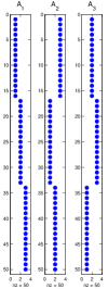
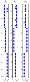
Original $\boldsymbol{\mathcal{C}}$

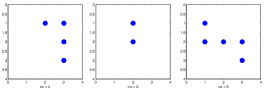
APG’s $\boldsymbol{\mathcal{C}}$

6 Conclusions

Sparse NTD aims at decomposing a tensor into the product of a core tensor and some factor matrices with nonnegativity and sparsity constraints. Existing algorithms for this problem either converge rapidly with very expensive per-iteration cost or have low per-iteration cost with very slow convergence speed. We have proposed the APG method, which owns both low per-iteration complexity and fast convergence speed. Moreover, the algorithm has been modified for sparse NTD from partial observations of a target tensor. The modified algorithm also has low per-iteration cost and can give similar decompositions from half of or even fewer observations as those from full observations.

Appendix A Efficient computation

The most expensive step in Algorithm 1 is the computation of $\nabla_{\boldsymbol{\mathcal{C}}}\ell(\boldsymbol{\mathcal{C}},\mathbf{A})$ and $\nabla_{\mathbf{A}_{n}}\ell(\boldsymbol{\mathcal{C}},{\mathbf{A}})$ in (13) and (14), respectively. Note that we have omitted the superscript. Next, we discuss how to efficiently compute them.

Computation of $\nabla_{\boldsymbol{\mathcal{C}}}\ell$

According to (2), we have

$$\ell(\boldsymbol{\mathcal{C}},\mathbf{A})=\frac{1}{2}\big{\|}\big{(}\otimes_{n=N}^{1}\mathbf{A}_{n}\big{)}\mathrm{vec}(\boldsymbol{\mathcal{C}})-\mathrm{vec}(\boldsymbol{\mathcal{M}})\big{\|}_{2}^{2}.$$

Using the properties of Kronecker product (see [14], for example), we have

$$\mathrm{vec}\big{(}\nabla_{\boldsymbol{\mathcal{C}}}\ell(\boldsymbol{\mathcal{C}},\mathbf{A})\big{)}=\big{(}\otimes_{n=N}^{1}\mathbf{A}_{n}^{\top}\mathbf{A}_{n}\big{)}\mathrm{vec}(\boldsymbol{\mathcal{C}})-\big{(}\otimes_{n=N}^{1}\mathbf{A}_{n}^{\top}\big{)}\mathrm{vec}(\boldsymbol{\mathcal{M}}).$$ (35)

It is extremely expensive to explicitly reformulate the Kronecker products in (35). Fortunately, we can use (2) again to have

$$\big{(}\otimes_{n=N}^{1}\mathbf{A}_{n}^{\top}\mathbf{A}_{n}\big{)}\mathrm{vec}(\boldsymbol{\mathcal{C}})=\mathrm{vec}\big{(}\boldsymbol{\mathcal{C}}\times_{1}\mathbf{A}_{1}^{\top}\mathbf{A}_{1}\cdots\times_{N}\mathbf{A}_{N}^{\top}\mathbf{A}_{N}\big{)}$$

and

$$\big{(}\otimes_{n=N}^{1}\mathbf{A}_{n}^{\top}\big{)}\mathrm{vec}(\boldsymbol{\mathcal{M}})=\mathrm{vec}\big{(}\boldsymbol{\mathcal{M}}\times_{1}\mathbf{A}_{1}^{\top}\cdots\times_{N}\mathbf{A}_{N}^{\top}\big{)}.$$

Hence, we have from (35) and the above two equalities that

$$\nabla_{\boldsymbol{\mathcal{C}}}\ell(\boldsymbol{\mathcal{C}},\mathbf{A})=\boldsymbol{\mathcal{C}}\times_{1}\mathbf{A}_{1}^{\top}\mathbf{A}_{1}\cdots\times_{N}\mathbf{A}_{N}^{\top}\mathbf{A}_{N}-\boldsymbol{\mathcal{M}}\times_{1}\mathbf{A}_{1}^{\top}\cdots\times_{N}\mathbf{A}_{N}^{\top}.$$ (36)

Computation of $\nabla_{\mathbf{A}_{n}}\ell$

According to (4), we have

$$\ell(\boldsymbol{\mathcal{C}},\mathbf{A})=\frac{1}{2}\big{\|}\mathbf{A}_{n}\mathbf{C}_{(n)}\big{(}\otimes_{\begin{subarray}{c}i=N\\ i\neq n\end{subarray}}^{1}\mathbf{A}_{i}\big{)}^{\top}-\mathbf{M}_{(n)}\big{\|}_{F}^{2}.$$ (37)

Hence,

$$\nabla_{\mathbf{A}_{n}}\ell(\boldsymbol{\mathcal{C}},\mathbf{A})=\mathbf{A}_{n}(\mathbf{B}_{n}\mathbf{B}_{n}^{\top})-\mathbf{M}_{(n)}\mathbf{B}_{n}^{\top}$$ (38)

where

$$\mathbf{B}_{n}=\mathbf{C}_{(n)}\big{(}\otimes_{\begin{subarray}{c}i=N\\ i\neq n\end{subarray}}^{1}\mathbf{A}_{i}\big{)}^{\top}.$$ (39)

Similar to what has been done to (35), we do not explicitly reformulate the Kronecker product in (39) but let

$$\boldsymbol{\mathcal{X}}=\boldsymbol{\mathcal{C}}\times_{1}\mathbf{A}_{1}\cdots\times_{n-1}\mathbf{A}_{n-1}\times_{n+1}\mathbf{A}_{n+1}\cdots\times_{N}\mathbf{A}_{N}.$$ (40)

Then we have $\mathbf{B}_{n}=\mathbf{X}_{(n)}$ according to (4).

Appendix B Complexity analysis of Algorithm 1

The main cost of Algorithm 1 lies in computing $\nabla_{\boldsymbol{\mathcal{C}}}\ell(\boldsymbol{\mathcal{C}},\mathbf{A})$ and $\nabla_{\mathbf{A}_{n}}\ell(\boldsymbol{\mathcal{C}},\mathbf{A})$, which are required in (13) and (14), respectively. Note that we have omitted all superscripts for simplicity. Through (36), the computation of $\nabla_{\boldsymbol{\mathcal{C}}}\ell(\boldsymbol{\mathcal{C}},\mathbf{A})$ requires

$$C\left(\sum_{j=1}^{N}R_{j}^{2}I_{j}+\sum_{j=1}^{N}R_{j}\prod_{i=1}^{N}R_{i}+\sum_{j=1}^{N}\big{(}\prod_{i=1}^{j}R_{i}\big{)}\big{(}\prod_{i=j}^{N}I_{i}\big{)}\right)$$ (41)

flops, where $C\approx 2$, the first part comes from the computation of all $\mathbf{A}_{i}^{\top}\mathbf{A}_{i}$’s, and the second and third parts are respectively from the computations of the first and second terms in (36). Disregarding the time for unfolding a tensor and using (38), we have the cost for $\nabla_{\mathbf{A}_{n}}\ell(\boldsymbol{\mathcal{C}},\mathbf{A})$ to be

$$C\left(\underset{\text{part 1}}{\underbrace{\sum_{j=1}^{n-1}\big{(}\prod_{i=1}^{j}I_{i}\big{)}\big{(}\prod_{i=j}^{N}R_{i}\big{)}+R_{n}\big{(}\prod_{i=1}^{n-1}I_{i}\big{)}\sum_{j=n+1}^{N}\big{(}\prod_{i=n+1}^{j}I_{i}\big{)}\big{(}\prod_{i=j}^{N}R_{i}\big{)}}}\right.$$ (42)

$$\hskip 28.45274pt\left.+\underset{\text{part 2}}{\underbrace{R_{n}^{2}\prod_{i\neq n}I_{i}+R_{n}^{2}I_{n}}}+\underset{\text{part 3}}{\underbrace{R_{n}\prod_{i=1}^{N}I_{i}}}\right),$$ (43)

where $C$ is the same as that in (41), “part 1” is for the computation of $\mathbf{B}_{n}$ via (40), “part 2” and “part 3” are respectively from the computations of the first and second terms in (38).

Suppose $R_{i}<I_{i}$ for all $i=1,\cdots,N$. Then the quantity of (41) is dominated by the third part because in this case,

$$R_{j}^{2}I_{j}<\big{(}\prod_{i=1}^{j}R_{i}\big{)}\big{(}\prod_{i=j}^{N}I_{i}\big{)},\qquad R_{j}\prod_{i=1}^{N}R_{i}<\big{(}\prod_{i=1}^{j}R_{i}\big{)}\big{(}\prod_{i=j}^{N}I_{i}\big{)}.$$

The quantity of (42) is dominated by the first and third parts. Only taking account of the dominating terms, we claim that the quantities of (41) and (42) are similar. To see this, assume $R_{i}=R,I_{i}=I,$ for all $i$’s. Then the third part of (41) is $\sum_{j=1}^{N}R^{j}I^{N-j+1}$, and the sum of the first and third parts of (42) is

$$\sum_{j=1}^{n-1}\big{(}\prod_{i=1}^{j}I_{i}\big{)}\big{(}\prod_{i=j}^{N}R_{i}\big{)}+R_{n}\big{(}\prod_{i=1}^{n-1}I_{i}\big{)}\sum_{j=n+1}^{N}\big{(}\prod_{i=n+1}^{j}I_{i}\big{)}\big{(}\prod_{i=j}^{N}R_{i}\big{)}+R_{n}\prod_{i=1}^{N}I_{i}$$

$$= \sum_{j=1}^{n-1}I^{j}R^{N-j+1}+\sum_{j=n+1}^{N}I^{j-1}R^{N-j+2}+RI^{N}$$

$$= \sum_{j=N-n+2}^{N}R^{j}I^{N-j+1}+\sum_{j=2}^{N-n+1}R^{j}I^{N-j+1}+RI^{N}$$

$$= \sum_{j=1}^{N}R^{j}I^{N-j+1}.$$

Hence, the costs for computing $\nabla_{\boldsymbol{\mathcal{C}}}\ell(\boldsymbol{\mathcal{C}},\mathbf{A})$ and $\nabla_{\mathbf{A}_{n}}\ell(\boldsymbol{\mathcal{C}},\mathbf{A})$ are similar.

After obtaining the partial gradients $\nabla_{\boldsymbol{\mathcal{C}}}\ell(\boldsymbol{\mathcal{C}},\mathbf{A})$ and $\nabla_{\mathbf{A}_{n}}\ell(\boldsymbol{\mathcal{C}},\mathbf{A})$, it remains to do some projections to nonnegative orthant to finish the updates in (13) and (14), and the cost is proportional to the size of $\boldsymbol{\mathcal{C}}$ and $\mathbf{A}_{n}$, i.e., $C_{p}\prod_{i=1}^{N}R_{i}$ and $C_{p}I_{n}R_{n}$ with $C_{p}\approx 4$. The data fitting term can be evaluated by

$$\ell(\boldsymbol{\mathcal{C}},\mathbf{A})=\frac{1}{2}\left(\langle\mathbf{A}_{n}^{\top}\mathbf{A}_{n},\mathbf{B}_{n}\mathbf{B}_{n}^{\top}\rangle-2\langle\mathbf{A}_{n},\mathbf{M}_{(n)}\mathbf{B}_{n}^{\top}\rangle+\|\boldsymbol{\mathcal{M}}\|_{F}^{2}\right),$$

where $\mathbf{B}_{n}$ is defined in (39). Note that $\mathbf{A}_{n}^{\top}\mathbf{A}_{n}$, $\mathbf{B}_{n}\mathbf{B}_{n}^{\top}$ and $\mathbf{M}_{(n)}\mathbf{B}_{n}^{\top}$ have been obtained during the computation of $\nabla_{\boldsymbol{\mathcal{C}}}\ell(\boldsymbol{\mathcal{C}},\mathbf{A})$ and $\nabla_{\mathbf{A}_{n}}\ell(\boldsymbol{\mathcal{C}},\mathbf{A})$, and $\|\boldsymbol{\mathcal{M}}\|_{F}^{2}$ can be pre-computed before running the algorithm. Hence, we need $C(R_{n}^{2}+I_{n}R_{n})$ additional flops to evaluate $\ell(\boldsymbol{\mathcal{C}},\mathbf{A})$, where $C\approx 2$. To get the objective value, we need $C(\prod_{i=1}^{N}R_{i}+\sum_{i=1}^{N}I_{i}R_{i})$ more flops for the regularization terms.

Some more computations occur in choosing Lipschitz constants $L_{c}$ and $L_{n}$’s. When $R_{n}\ll I_{n}$ for all $n$, the cost for computing Lipschitz constants, projection to nonnegative orthant and objective evaluation is negligible compared to that for computing partial gradients $\nabla_{\boldsymbol{\mathcal{C}}}\ell(\boldsymbol{\mathcal{C}},\mathbf{A})$ and $\nabla_{\mathbf{A}_{n}}\ell(\boldsymbol{\mathcal{C}},\mathbf{A})$. Omitting the negligible cost and only accounting the main cost in (41) and (42), the per-iteration complexity of Algorithm 1 is

$$N\cdot\mathcal{O}\left(\sum_{j=1}^{N}\big{(}\prod_{i=1}^{j}R_{i}\big{)}\big{(}\prod_{i=j}^{N}I_{i}\big{)}+\sum_{j=1}^{N}\big{(}\prod_{i=1}^{j}I_{i}\big{)}\big{(}\prod_{i=j}^{N}R_{i}\big{)}\right).$$ (44)

Appendix C Proof of Theorem 2

C.1 Subsequence convergence

First, we give a subsequence convergence result, namely, any limit point of $\{\boldsymbol{\mathcal{W}}^{k}\}$ is a stationary point. Using Lemma 2.1 of [35], we have

$$F(\boldsymbol{\mathcal{C}}^{k,n-1},\mathbf{A}_{j<n}^{k},\mathbf{A}_{j\geq n}^{k-1})-F(\boldsymbol{\mathcal{C}}^{k,n},\mathbf{A}_{j<n}^{k},\mathbf{A}_{j\geq n}^{k-1})$$ (45)

$$\geq \frac{L_{c}^{k,n}}{2}\|\hat{\boldsymbol{\mathcal{C}}}^{k,n}-\boldsymbol{\mathcal{C}}^{k,n}\|_{F}^{2}+L_{c}^{k,n}\left\langle\hat{\boldsymbol{\mathcal{C}}}^{k,n}-\boldsymbol{\mathcal{C}}^{k,n-1},\boldsymbol{\mathcal{C}}^{k,n}-\hat{\boldsymbol{\mathcal{C}}}^{k,n}\right\rangle$$ (46)

$$= \frac{L_{c}^{k,n}}{2}\|\boldsymbol{\mathcal{C}}^{k,n-1}-\boldsymbol{\mathcal{C}}^{k,n}\|_{F}^{2}-\frac{L_{c}^{k,n}}{2}(\omega_{c}^{k,n})^{2}\|\boldsymbol{\mathcal{C}}^{k,n-2}-\boldsymbol{\mathcal{C}}^{k,n-1}\|_{F}^{2}$$ (47)

$$\geq \frac{L_{c}^{k,n}}{2}\|\boldsymbol{\mathcal{C}}^{k,n-1}-\boldsymbol{\mathcal{C}}^{k,n}\|_{F}^{2}-\frac{L_{c}^{k,n-1}}{2}\delta_{\omega}^{2}\|\boldsymbol{\mathcal{C}}^{k,n-2}-\boldsymbol{\mathcal{C}}^{k,n-1}\|_{F}^{2},$$ (48)

where we have used $\omega_{c}^{k,n}\leq\delta_{\omega}\sqrt{\frac{L_{c}^{k,n-1}}{L_{c}^{k,n}}}$ to get the last inequality. Note that if the re-update in Line 1 is performed, then $\omega_{c}^{k,n}=0$ in (47), and (48) still holds. Similarly, we have

$$\begin{array}[]{ll}&F(\boldsymbol{\mathcal{C}}^{k,n},\mathbf{A}_{j<n}^{k},\mathbf{A}_{j\geq n}^{k-1})-F(\boldsymbol{\mathcal{C}}^{k,n},\mathbf{A}_{j\leq n}^{k},\mathbf{A}_{j>n}^{k-1})\\[2.84544pt] \geq&\frac{L_{n}^{k}}{2}\|\mathbf{A}_{n}^{k-1}-\mathbf{A}_{n}^{k}\|_{F}^{2}-\frac{L_{n}^{k-1}}{2}\delta_{\omega}^{2}\|\mathbf{A}_{n}^{k-2}-\mathbf{A}_{n}^{k-1}\|_{F}^{2}.\end{array}$$ (49)

Summing (48) and (49) together over $n$ and noting $\boldsymbol{\mathcal{C}}^{k,-1}=\boldsymbol{\mathcal{C}}^{k-1,N-1},\boldsymbol{\mathcal{C}}^{k,0}=\boldsymbol{\mathcal{C}}^{k-1,N}$ yield

$$F(\boldsymbol{\mathcal{W}}^{k-1})-F(\boldsymbol{\mathcal{W}}^{k})$$ (50)

$$\geq \sum_{n=1}^{N}\left(\frac{L_{c}^{k,n}}{2}\|\boldsymbol{\mathcal{C}}^{k,n-1}-\boldsymbol{\mathcal{C}}^{k,n}\|_{F}^{2}-\frac{L_{c}^{k,n-1}}{2}\delta_{\omega}^{2}\|\boldsymbol{\mathcal{C}}^{k,n-2}-\boldsymbol{\mathcal{C}}^{k,n-1}\|_{F}^{2}\right.$$ (51)

$$\hskip 22.76228pt\left.+\frac{L_{n}^{k}}{2}\|\mathbf{A}_{n}^{k-1}-\mathbf{A}_{n}^{k}\|_{F}^{2}-\frac{L_{n}^{k-1}}{2}\delta_{\omega}^{2}\|\mathbf{A}_{n}^{k-2}-\mathbf{A}_{n}^{k-1}\|_{F}^{2}\right)$$ (52)

$$= \frac{L_{c}^{k,N}}{2}\|\boldsymbol{\mathcal{C}}^{k,N-1}-\boldsymbol{\mathcal{C}}^{k,N}\|_{F}^{2}-\frac{L_{c}^{k-1,N}}{2}\delta_{\omega}^{2}\|\boldsymbol{\mathcal{C}}^{k-1,N-1}-\boldsymbol{\mathcal{C}}^{k-1,N}\|_{F}^{2}$$ (53)

$$+\sum_{n=1}^{N-1}\frac{(1-\delta_{\omega}^{2})L_{c}^{k,n}}{2}\|\boldsymbol{\mathcal{C}}^{k,n-1}-\boldsymbol{\mathcal{C}}^{k,n}\|_{F}^{2}$$ (54)

$$+\sum_{n=1}^{N}\left(\frac{L_{n}^{k}}{2}\|\mathbf{A}_{n}^{k-1}-\mathbf{A}_{n}^{k}\|_{F}^{2}-\frac{L_{n}^{k-1}}{2}\delta_{\omega}^{2}\|\mathbf{A}_{n}^{k-2}-\mathbf{A}_{n}^{k-1}\|_{F}^{2}\right).$$

Summing (53) over $k$, we have

$$F(\boldsymbol{\mathcal{W}}^{0})-F(\boldsymbol{\mathcal{W}}^{K})$$ (55)

$$\geq \sum_{k=1}^{K}\sum_{n=1}^{N}\left(\frac{(1-\delta_{\omega}^{2})L_{c}^{k,n}}{2}\|\boldsymbol{\mathcal{C}}^{k,n-1}-\boldsymbol{\mathcal{C}}^{k,n}\|_{F}^{2}+\frac{(1-\delta_{\omega}^{2})L_{n}^{k}}{2}\|\mathbf{A}_{n}^{k-1}-\mathbf{A}_{n}^{k}\|_{F}^{2}\right)$$ (56)

$$\geq \frac{(1-\delta_{\omega}^{2})L_{d}}{2}\sum_{k=1}^{K}\sum_{n=1}^{N}\left(\|\boldsymbol{\mathcal{C}}^{k,n-1}-\boldsymbol{\mathcal{C}}^{k,n}\|_{F}^{2}+\|\mathbf{A}_{n}^{k-1}-\mathbf{A}_{n}^{k}\|_{F}^{2}\right).$$ (57)

Letting $K\to\infty$ and observing $F$ is lower bounded, we have

$$\sum_{k=1}^{\infty}\sum_{n=1}^{N}\left(\|\boldsymbol{\mathcal{C}}^{k,n-1}-\boldsymbol{\mathcal{C}}^{k,n}\|_{F}^{2}+\|\mathbf{A}_{n}^{k-1}-\mathbf{A}_{n}^{k}\|_{F}^{2}\right)<\infty.$$ (58)

Suppose $\bar{\boldsymbol{\mathcal{W}}}=(\bar{\boldsymbol{\mathcal{C}}},\bar{\mathbf{A}}_{1},\cdots,\bar{\mathbf{A}}_{N})$ is a limit point of $\{\boldsymbol{\mathcal{W}}^{k}\}$. Then there is a subsequence $\{\boldsymbol{\mathcal{W}}^{k^{\prime}}\}$ converging to $\bar{\boldsymbol{\mathcal{W}}}$. Since $\{L_{c}^{k,n},L_{n}^{k}\}$ is bounded, passing another subsequence if necessary, we assume $L_{c}^{k^{\prime},n}\to\bar{L}_{c}^{n}$ and $L_{n}^{k^{\prime}}\to\bar{L}_{n}$. Note that (58) implies $\mathbf{A}^{k^{\prime}-1}\to\bar{\mathbf{A}}$ and $\boldsymbol{\mathcal{C}}^{m,n}\to\bar{\boldsymbol{\mathcal{C}}}$ for all $n$ and $m=k^{\prime},k^{\prime}-1,k^{\prime}-2$, as $k\to\infty$. Hence, $\hat{\boldsymbol{\mathcal{C}}}^{k^{\prime},n}\to\bar{\boldsymbol{\mathcal{C}}}$ for all $n$, as $k\to\infty$. Recall that

$$\boldsymbol{\mathcal{C}}^{k^{\prime},n}=\operatorname*{argmin}_{\boldsymbol{\mathcal{C}}\geq 0}\left\langle\nabla_{\boldsymbol{\mathcal{C}}}\ell(\hat{\boldsymbol{\mathcal{C}}}^{k^{\prime},n},\mathbf{A}_{j<n}^{k^{\prime}},\mathbf{A}_{j\geq n}^{k^{\prime}-1}),\boldsymbol{\mathcal{C}}-\hat{\boldsymbol{\mathcal{C}}}^{k^{\prime},n}\right\rangle+\frac{L_{c}^{k^{\prime},n}}{2}\|\boldsymbol{\mathcal{C}}-\hat{\boldsymbol{\mathcal{C}}}^{k^{\prime},n}\|_{F}^{2}+\lambda_{c}\|\boldsymbol{\mathcal{C}}\|_{1}.$$ (59)

Letting $k\to\infty$ and using the continuity of the objective in (59) give

$$\bar{\boldsymbol{\mathcal{C}}}=\operatorname*{argmin}_{\boldsymbol{\mathcal{C}}\geq 0}\left\langle\nabla_{\boldsymbol{\mathcal{C}}}\ell(\bar{\boldsymbol{\mathcal{C}}},\bar{\mathbf{A}}),\boldsymbol{\mathcal{C}}-\bar{\boldsymbol{\mathcal{C}}}\right\rangle+\frac{\bar{L}_{c}^{n}}{2}\|\boldsymbol{\mathcal{C}}-\bar{\boldsymbol{\mathcal{C}}}\|_{F}^{2}+\lambda_{c}\|\boldsymbol{\mathcal{C}}\|_{1}.$$

Hence, $\bar{\boldsymbol{\mathcal{C}}}$ satisfies the first-order optimality condition

$$\left\langle\nabla_{\boldsymbol{\mathcal{C}}}\ell(\bar{\boldsymbol{\mathcal{C}}},\bar{\mathbf{A}})+\lambda_{c}\boldsymbol{\mathcal{P}}_{c},\boldsymbol{\mathcal{C}}-\bar{\boldsymbol{\mathcal{C}}}\right\rangle\geq 0,~{}\text{for all }\boldsymbol{\mathcal{C}}\geq 0,\text{ some }\boldsymbol{\mathcal{P}}_{c}\in\partial\|\bar{\boldsymbol{\mathcal{C}}}\|_{1}.$$ (60)

Similarly, we have for all $n$ that

$$\left\langle\nabla_{\mathbf{A}_{n}}\ell(\bar{\boldsymbol{\mathcal{C}}},\bar{\mathbf{A}})+\lambda_{n}\boldsymbol{\mathbf{P}}_{n},\mathbf{A}_{n}-\bar{\mathbf{A}}_{n}\right\rangle\geq 0,~{}\text{for all }\mathbf{A}_{n}\geq 0,\text{ some }\boldsymbol{\mathbf{P}}_{n}\in\partial\|\bar{\mathbf{A}}_{n}\|_{1}.$$ (61)

Note (60) together with (61) gives the first-order optimality conditions of (5). Hence, $\bar{\boldsymbol{\mathcal{W}}}$ is a stationary point.

C.2 Global convergence

Next we show the entire sequence $\{\boldsymbol{\mathcal{W}}^{k}\}$ converges to a limit point $\bar{\boldsymbol{\mathcal{W}}}$. Since all $\lambda_{c},\lambda_{1},\cdots,\lambda_{N}$ are positive, the sequence $\{\boldsymbol{\mathcal{W}}^{k}\}$ is bounded and admits a finite limit point $\bar{\boldsymbol{\mathcal{W}}}$. Let $E=\{\boldsymbol{\mathcal{W}}:\|\boldsymbol{\mathcal{W}}\|_{F}\leq 4\nu\}$, where $\|\boldsymbol{\mathcal{W}}\|_{F}\triangleq\sqrt{\|\boldsymbol{\mathcal{C}}\|_{F}^{2}+\|\mathbf{A}\|_{F}^{2}}$ and $\nu$ is a constant such that $\|(\boldsymbol{\mathcal{C}}^{k,n},\mathbf{A}^{k})\|_{F}\leq\nu$ for all $k,n$. Let $L_{G}$ be a uniform Lipschitz constant of $\nabla_{\boldsymbol{\mathcal{C}}}\ell(\boldsymbol{\mathcal{W}})$ and $\nabla_{\mathbf{A}_{n}}\ell(\boldsymbol{\mathcal{W}}),n=1,\cdots,N,$ over $E$, namely,

$$\|\nabla_{\boldsymbol{\mathcal{C}}}\ell(\boldsymbol{\mathcal{Y}})-\nabla_{\boldsymbol{\mathcal{C}}}\ell(\boldsymbol{\mathcal{Z}})\|_{F}\leq L_{G}\|\boldsymbol{\mathcal{Y}}-\boldsymbol{\mathcal{Z}}\|_{F},~{}\forall\boldsymbol{\mathcal{Y}},\boldsymbol{\mathcal{Z}}\in E,$$ (62a)

$$\|\nabla_{\mathbf{A}_{n}}\ell(\boldsymbol{\mathcal{Y}})-\nabla_{\mathbf{A}_{n}}\ell(\boldsymbol{\mathcal{Z}})\|_{F}\leq L_{G}\|\boldsymbol{\mathcal{Y}}-\boldsymbol{\mathcal{Z}}\|_{F},~{}\forall\boldsymbol{\mathcal{Y}},\boldsymbol{\mathcal{Z}}\in E,~{}\forall n,$$ (62b)

Let

$$H(\boldsymbol{\mathcal{C}},\mathbf{A})=\ell(\boldsymbol{\mathcal{C}},\mathbf{A})+\lambda_{c}\|\boldsymbol{\mathcal{C}}\|_{1}+\delta_{+}(\boldsymbol{\mathcal{C}})+\overset{N}{\underset{n=1}{\sum}}\big{(}\lambda_{n}\|\mathbf{A}_{n}\|_{1}+\delta_{+}(\mathbf{A}_{n})\big{)}$$

and

$$r_{c}(\boldsymbol{\mathcal{C}})=\lambda_{c}\|\boldsymbol{\mathcal{C}}\|_{1}+\delta_{+}(\boldsymbol{\mathcal{C}}),\quad r_{n}(\mathbf{A}_{n})=\lambda_{n}\|\mathbf{A}_{n}\|_{1}+\delta_{+}(\mathbf{A}_{n}),\ n=1,\cdots,N,$$

where $\delta_{+}(\cdot)$ is the indicator function on nonnegative orthant, namely, it equals zero if the argument is component-wise nonnegative and $+\infty$ otherwise.

Note that (5) is equivalent to

$$\min_{\boldsymbol{\mathcal{C}},\mathbf{A}}H(\boldsymbol{\mathcal{C}},\mathbf{A}).$$ (63)

Recall that $H$ satisfies the KL property (see [25, 4] for example) at $\bar{\boldsymbol{\mathcal{W}}}$, namely, there exist $\gamma,\rho>0$, $\theta\in[0,1)$, and a neighborhood $B(\bar{\boldsymbol{\mathcal{W}}},\rho)\triangleq\{\boldsymbol{\mathcal{W}}:\|\boldsymbol{\mathcal{W}}-\bar{\boldsymbol{\mathcal{W}}}\|_{F}\leq\rho\}$ such that

$$|H(\boldsymbol{\mathcal{W}})-H(\bar{\boldsymbol{\mathcal{W}}})|^{\theta}\leq\gamma\cdot\text{dist}(\mathbf{0},\partial H(\boldsymbol{\mathcal{W}})),~{}\text{for all }\boldsymbol{\mathcal{W}}\in B(\bar{\boldsymbol{\mathcal{W}}},\rho).$$ (64)

Denote $H_{k}=H(\boldsymbol{\mathcal{W}}^{k})-H(\bar{\boldsymbol{\mathcal{W}}})$. Then $H_{k}\downarrow 0$. Since $\bar{\boldsymbol{\mathcal{W}}}$ is a limit point of $\{\boldsymbol{\mathcal{W}}^{k}\}$ and $\|\mathbf{A}^{k}-\mathbf{A}^{k+1}\|_{F}\to 0,\|\boldsymbol{\mathcal{C}}^{k,n-1}-\boldsymbol{\mathcal{C}}^{k,n}\|_{F}\to 0$ for all $k,n$ from (58), for any $T>0$, there must exist $k_{0}$ such that $\boldsymbol{\mathcal{W}}^{j}\in B(\bar{\boldsymbol{\mathcal{W}}},\rho),j=k_{0},k_{0}+1,k_{0}+2$ and

$$T\big{(}H_{k_{0}}^{1-\theta}+\|\mathbf{A}^{k_{0}}-\mathbf{A}^{k_{0}+1}\|_{F}+\|\mathbf{A}^{k_{0}+1}-\mathbf{A}^{k_{0}+2}\|_{F}+\|\boldsymbol{\mathcal{C}}^{k_{0}+2,N-1}-\boldsymbol{\mathcal{C}}^{k_{0}+2,N}\|_{F}\big{)}$$

$$\hskip 8.5359pt+\|\boldsymbol{\mathcal{W}}^{k_{0}+2}-\bar{\boldsymbol{\mathcal{W}}}\|_{F}<\rho.$$

Take $T$ as specified in (97) and consider the sequence $\{\boldsymbol{\mathcal{W}}^{k}\}_{k\geq k_{0}}$, which is equivalent to starting the algorithm from $\boldsymbol{\mathcal{W}}^{k_{0}}$ and, thus without loss of generality, let $k_{0}=0$, namely, $\boldsymbol{\mathcal{W}}^{j}\in B(\bar{\boldsymbol{\mathcal{W}}},\rho),j=0,1,2$, and

$$T\big{(}H_{0}^{1-\theta}+\|\mathbf{A}^{0}-\mathbf{A}^{1}\|_{F}+\|\mathbf{A}^{1}-\mathbf{A}^{2}\|_{F}+\|\boldsymbol{\mathcal{C}}^{2,N-1}-\boldsymbol{\mathcal{C}}^{2,N}\|_{F}\big{)}+\|\boldsymbol{\mathcal{W}}^{2}-\bar{\boldsymbol{\mathcal{W}}}\|_{F}<\rho.$$ (65)

The idea of our proof is to show

$$\boldsymbol{\mathcal{W}}^{k}\in B(\bar{\boldsymbol{\mathcal{W}}},\rho),~{}\text{for all }k,$$ (66)

and employ the KL inequality (64) to show $\{\boldsymbol{\mathcal{W}}^{k}\}$ is a Cauchy sequence, thus the entire sequence converges. Assume $\boldsymbol{\mathcal{W}}^{k}\in B(\bar{\boldsymbol{\mathcal{W}}},\rho)$ for $0\leq k\leq K$. We go to show $\boldsymbol{\mathcal{W}}^{K+1}\in B(\bar{\boldsymbol{\mathcal{W}}},\rho)$ and conclude (66) by induction.

Note that

$$\partial H(\boldsymbol{\mathcal{W}}^{k})=\left\{\partial r_{1}(\mathbf{A}_{1}^{k})+\nabla_{\mathbf{A}_{1}}\ell(\boldsymbol{\mathcal{W}}^{k})\right\}\times\cdots\times\left\{\partial r_{N}(\mathbf{A}_{N}^{k})+\nabla_{\mathbf{A}_{N}}\ell(\boldsymbol{\mathcal{W}}^{k})\right\}\times\left\{\partial r_{c}(\boldsymbol{\mathcal{C}}^{k,N})+\nabla_{\boldsymbol{\mathcal{C}}}\ell(\boldsymbol{\mathcal{W}}^{k})\right\},$$

and for all $n$ and $k$

$$-L_{n}^{k}(\mathbf{A}_{n}^{k}-\hat{\mathbf{A}}_{n}^{k})-\nabla_{\mathbf{A}_{n}}\ell(\boldsymbol{\mathcal{C}}^{k,n},\mathbf{A}_{j<n}^{k},\hat{\mathbf{A}}_{n}^{k},\mathbf{A}_{j\geq n}^{k-1})+\nabla_{\mathbf{A}_{n}}\ell(\boldsymbol{\mathcal{W}}^{k})\in \partial r_{n}(\mathbf{A}_{n}^{k})+\nabla_{\mathbf{A}_{n}}\ell(\boldsymbol{\mathcal{W}}^{k}),$$

$$-L_{c}^{k,N}(\boldsymbol{\mathcal{C}}^{k,N}-\hat{\boldsymbol{\mathcal{C}}}^{k,N})-\nabla_{\boldsymbol{\mathcal{C}}}\ell(\hat{\boldsymbol{\mathcal{C}}}^{k,N},\mathbf{A}_{j<N}^{k},{\mathbf{A}}_{N}^{k-1})+\nabla_{\boldsymbol{\mathcal{C}}}\ell(\boldsymbol{\mathcal{W}}^{k})\in \partial r_{c}(\boldsymbol{\mathcal{C}}^{k,N})+\nabla_{\boldsymbol{\mathcal{C}}}\ell(\boldsymbol{\mathcal{W}}^{k}).$$

Hence, for all $k\leq K$,

$$\text{dist}\big{(}\mathbf{0},\partial H(\boldsymbol{\mathcal{W}}^{k})\big{)}$$ (67)

$$\leq \big{\|}(L_{1}^{k}(\mathbf{A}_{1}^{k}-\hat{\mathbf{A}}_{1}^{k}),\cdots,L_{1}^{k}(\mathbf{A}_{1}^{k}-\hat{\mathbf{A}}_{1}^{k}),L_{c}^{k,n}(\boldsymbol{\mathcal{C}}^{k,N}-\hat{\boldsymbol{\mathcal{C}}}^{k,N}))\big{\|}_{F}$$ (68)

$$+\sum_{n=1}^{N}\big{\|}\nabla_{\mathbf{A}_{n}}\ell(\boldsymbol{\mathcal{C}}^{k,n},\mathbf{A}_{j<n}^{k},\hat{\mathbf{A}}_{n}^{k},\mathbf{A}_{j\geq n}^{k-1})-\nabla_{\mathbf{A}_{n}}\ell(\boldsymbol{\mathcal{W}}^{k})\big{\|}_{F}$$ (69)

$$+\big{\|}\nabla_{\boldsymbol{\mathcal{C}}}\ell(\hat{\boldsymbol{\mathcal{C}}}^{k,N},\mathbf{A}_{j<N}^{k},{\mathbf{A}}_{N}^{k-1})-\nabla_{\boldsymbol{\mathcal{C}}}\ell(\boldsymbol{\mathcal{W}}^{k})\big{\|}_{F}$$ (70)

$$\leq L_{u}\big{(}\|\mathbf{A}^{k}-\mathbf{A}^{k-1}\|_{F}+\|\mathbf{A}^{k-1}-\mathbf{A}^{k-2}\|_{F}\big{)}+L_{u}\big{(}\|\boldsymbol{\mathcal{C}}^{k,N}-\boldsymbol{\mathcal{C}}^{k,N-1}\|_{F}+\|\boldsymbol{\mathcal{C}}^{k,N-1}-\boldsymbol{\mathcal{C}}^{k,N-2}\|_{F}\big{)}$$ (71)

$$+\sum_{n=1}^{N}L_{G}\big{(}\|\boldsymbol{\mathcal{C}}^{k,n}-\boldsymbol{\mathcal{C}}^{k,N}\|_{F}+\|\mathbf{A}^{k}-\mathbf{A}^{k-1}\|_{F}+\|\mathbf{A}^{k-1}-\mathbf{A}^{k-2}\|_{F}\big{)}$$ (72)

$$+L_{G}\big{(}\|\boldsymbol{\mathcal{C}}^{k,N}-\boldsymbol{\mathcal{C}}^{k,N-1}\|_{F}+\|\boldsymbol{\mathcal{C}}^{k,N-1}-\boldsymbol{\mathcal{C}}^{k,N-2}\|_{F}+\|\mathbf{A}^{k}-\mathbf{A}^{k-1}\|_{F}\big{)}$$ (73)

$$\leq \big{(}L_{u}+(N+1)L_{G}\big{)}\left(\|\mathbf{A}^{k}-\mathbf{A}^{k-1}\|_{F}+\|\mathbf{A}^{k-1}-\mathbf{A}^{k-2}\|_{F}\right.$$ (74)

$$\hskip 22.76228pt\left.+\|\boldsymbol{\mathcal{C}}^{k,N}-\boldsymbol{\mathcal{C}}^{k,N-1}\|_{F}+\sum_{n=1}^{N-1}\|\boldsymbol{\mathcal{C}}^{k,n-1}-\boldsymbol{\mathcal{C}}^{k,n}\|_{F}\right),$$

where we have used $L_{n}^{k},L_{c}^{k,n}\leq L_{u},~{}\forall k,n$ and (62) to have the second inequality, and the third inequality is obtained from $\|\boldsymbol{\mathcal{C}}^{k,n}-\boldsymbol{\mathcal{C}}^{k,N}\|_{F}\leq\sum_{i=n}^{N-1}\|\boldsymbol{\mathcal{C}}^{k,i}-\boldsymbol{\mathcal{C}}^{k,i+1}\|_{F}$ and doing some simplification. Using the KL inequality (64) at $\boldsymbol{\mathcal{W}}=\boldsymbol{\mathcal{W}}^{k}$ and the inequality

$$\frac{s^{\theta}}{1-\theta}(s^{1-\theta}-t^{1-\theta})\geq s-t,~{}\forall s,t\geq 0,$$

we get

$$\frac{\gamma}{1-\theta}\text{dist}(\mathbf{0},\partial H(\boldsymbol{\mathcal{W}}^{k}))(H_{k}^{1-\theta}-H_{k+1}^{1-\theta})\geq H_{k}-H_{k+1}.$$ (75)

By (53), we have

$$H_{k}-H_{k+1}\geq \frac{L_{c}^{k+1,N}}{2}\|\boldsymbol{\mathcal{C}}^{k+1,N-1}-\boldsymbol{\mathcal{C}}^{k+1,N}\|_{F}^{2}-\frac{L_{c}^{k,N}}{2}\delta_{\omega}^{2}\|\boldsymbol{\mathcal{C}}^{k,N-1}-\boldsymbol{\mathcal{C}}^{k,N}\|_{F}^{2}$$ (76)

$$+\sum_{n=1}^{N-1}\frac{(1-\delta_{\omega}^{2})L_{c}^{k+1,n}}{2}\|\boldsymbol{\mathcal{C}}^{k+1,n-1}-\boldsymbol{\mathcal{C}}^{k+1,n}\|_{F}^{2}$$ (77)

$$+\sum_{n=1}^{N}\left(\frac{L_{n}^{k+1}}{2}\|\mathbf{A}_{n}^{k}-\mathbf{A}_{n}^{k+1}\|_{F}^{2}-\frac{L_{n}^{k}}{2}\delta_{\omega}^{2}\|\mathbf{A}_{n}^{k-1}-\mathbf{A}_{n}^{k}\|_{F}^{2}\right).$$

Combining (74), (75), (76) and noting $L_{c}^{k+1,n}\geq L_{d}$ yield

$$\frac{\gamma(L_{u}+(N+1)L_{G})}{1-\theta}(H_{k}^{1-\theta}-H_{k+1}^{1-\theta})\big{[}\|\mathbf{A}^{k}-\mathbf{A}^{k-1}\|_{F}+\|\mathbf{A}^{k-1}-\mathbf{A}^{k-2}\|_{F}$$ (78)

$$\hskip 113.81102pt+\|\boldsymbol{\mathcal{C}}^{k,N}-\boldsymbol{\mathcal{C}}^{k,N-1}\|_{F}+\sum_{n=1}^{N-1}\|\boldsymbol{\mathcal{C}}^{k,n-1}-\boldsymbol{\mathcal{C}}^{k,n}\|_{F}\big{]}$$ (79)

$$+\delta_{\omega}^{2}\left\|(\sqrt{L_{1}^{k}}\mathbf{A}_{1}^{k-1},\cdots,\sqrt{L_{N}^{k}}\mathbf{A}_{N}^{k-1},\sqrt{L_{c}^{k,N}}\boldsymbol{\mathcal{C}}^{k,N-1})\right.$$ (80)

$$\hskip 28.45274pt\left.-(\sqrt{L_{1}^{k}}\mathbf{A}_{1}^{k},\cdots,\sqrt{L_{N}^{k}}\mathbf{A}_{N}^{k},\sqrt{L_{c}^{k,N}}\boldsymbol{\mathcal{C}}^{k,N})\right\|_{F}^{2}$$ (81)

$$\geq \left\|(\sqrt{L_{1}^{k+1}}\mathbf{A}_{1}^{k},\cdots,\sqrt{L_{N}^{k+1}}\mathbf{A}_{N}^{k},\sqrt{L_{c}^{k+1,N}}\boldsymbol{\mathcal{C}}^{k+1,N-1})\right.$$ (82)

$$\hskip 11.38092pt\left.-(\sqrt{L_{1}^{k+1}}\mathbf{A}_{1}^{k+1},\cdots,\sqrt{L_{N}^{k+1}}\mathbf{A}_{N}^{k+1},\sqrt{L_{c}^{k+1,N}}\boldsymbol{\mathcal{C}}^{k+1,N})\right\|_{F}^{2}$$

$$+\frac{(1-\delta_{\omega}^{2})L_{d}}{2}\sum_{n=1}^{N-1}\|\boldsymbol{\mathcal{C}}^{k+1,n-1}-\boldsymbol{\mathcal{C}}^{k+1,n}\|_{F}^{2}.$$

By Cauchy-Schwart inequality, we estimate

$$\sqrt{\text{right side of inequality \eqref{eq:ineq5}}}$$

$$\geq \frac{1+\delta_{\omega}}{2}\left\|(\sqrt{L_{1}^{k+1}}\mathbf{A}_{1}^{k},\cdots,\sqrt{L_{N}^{k+1}}\mathbf{A}_{N}^{k},\sqrt{L_{c}^{k+1,N}}\boldsymbol{\mathcal{C}}^{k+1,N-1})\right.$$ (83)

$$\hskip 34.14322pt\left.-(\sqrt{L_{1}^{k+1}}\mathbf{A}_{1}^{k+1},\cdots,\sqrt{L_{N}^{k+1}}\mathbf{A}_{N}^{k+1},\sqrt{L_{c}^{k+1,N}}\boldsymbol{\mathcal{C}}^{k+1,N})\right\|_{F}$$

$$+\eta\sum_{n=1}^{N-1}\|\boldsymbol{\mathcal{C}}^{k+1,n-1}-\boldsymbol{\mathcal{C}}^{k+1,n}\|_{F},$$ (84)

where $\eta>0$ is sufficiently small and depends on $\delta_{\omega},L_{d},N$, and

$$\sqrt{\text{left side of inequality \eqref{eq:ineq5}}}$$ (85)

$$\leq \frac{\mu\gamma(L_{u}+(N+1)L_{G})}{4(1-\theta)}(H_{k}^{1-\theta}-H_{k+1}^{1-\theta})$$ (86)

$$+\frac{1}{\mu}\big{[}\|\mathbf{A}^{k}-\mathbf{A}^{k-1}\|_{F}+\|\mathbf{A}^{k-1}-\mathbf{A}^{k-2}\|_{F}+\|\boldsymbol{\mathcal{C}}^{k,N}-\boldsymbol{\mathcal{C}}^{k,N-1}\|_{F}+\sum_{n=1}^{N-1}\|\boldsymbol{\mathcal{C}}^{k,n-1}-\boldsymbol{\mathcal{C}}^{k,n}\|_{F}\big{]}$$ (87)

$$+\delta_{\omega}\left\|(\sqrt{L_{1}^{k}}\mathbf{A}_{1}^{k-1},\cdots,\sqrt{L_{N}^{k}}\mathbf{A}_{N}^{k-1},\sqrt{L_{c}^{k,N}}\boldsymbol{\mathcal{C}}^{k,N-1})-(\sqrt{L_{1}^{k}}\mathbf{A}_{1}^{k},\cdots,\sqrt{L_{N}^{k}}\mathbf{A}_{N}^{k},\sqrt{L_{c}^{k,N}}\boldsymbol{\mathcal{C}}^{k,N})\right\|_{F},$$

where $\mu>0$ is a sufficiently large constant such that $\frac{1}{\mu}<\min(\eta,\frac{1-\delta_{\omega}}{4}\sqrt{\frac{L_{d}}{2}}).$ Combining (82),(86), (84) and summing them over $k$ from $2$ to $K$ give

$$\frac{\mu\gamma(L_{u}+(N+1)L_{G})}{4(1-\theta)}(H_{2}^{1-\theta}-H_{K+1}^{1-\theta})$$ (88)

$$+\frac{1}{\mu}\sum_{k=2}^{K}\big{[}\|\mathbf{A}^{k}-\mathbf{A}^{k-1}\|_{F}+\|\mathbf{A}^{k-1}-\mathbf{A}^{k-2}\|_{F}+\|\boldsymbol{\mathcal{C}}^{k,N}-\boldsymbol{\mathcal{C}}^{k,N-1}\|_{F}+\sum_{n=1}^{N-1}\|\boldsymbol{\mathcal{C}}^{k,n-1}-\boldsymbol{\mathcal{C}}^{k,n}\|_{F}\big{]}$$ (89)

$$+\delta_{\omega}\sum_{k=2}^{K}\left\|(\sqrt{L_{1}^{k}}\mathbf{A}_{1}^{k-1},\cdots,\sqrt{L_{N}^{k}}\mathbf{A}_{N}^{k-1},\sqrt{L_{c}^{k,N}}\boldsymbol{\mathcal{C}}^{k,N-1})-(\sqrt{L_{1}^{k}}\mathbf{A}_{1}^{k},\cdots,\sqrt{L_{N}^{k}}\mathbf{A}_{N}^{k},\sqrt{L_{c}^{k,N}}\boldsymbol{\mathcal{C}}^{k,N})\right\|_{F}$$ (90)

$$\geq \frac{1+\delta_{\omega}}{2}\sum_{k=2}^{K}\left\|(\sqrt{L_{1}^{k+1}}\mathbf{A}_{1}^{k},\cdots,\sqrt{L_{N}^{k+1}}\mathbf{A}_{N}^{k},\sqrt{L_{c}^{k+1,N}}\boldsymbol{\mathcal{C}}^{k+1,N-1})\right.$$ (91)

$$\hskip 28.45274pt\left.-(\sqrt{L_{1}^{k+1}}\mathbf{A}_{1}^{k+1},\cdots,\sqrt{L_{N}^{k+1}}\mathbf{A}_{N}^{k+1},\sqrt{L_{c}^{k+1,N}}\boldsymbol{\mathcal{C}}^{k+1,N})\right\|_{F}+\eta\sum_{k=2}^{K}\sum_{n=1}^{N-1}\|\boldsymbol{\mathcal{C}}^{k+1,n-1}-\boldsymbol{\mathcal{C}}^{k+1,n}\|_{F}.$$

Simplifying the above inequality, we have

$$\frac{\mu\gamma(L_{u}+(N+1)L_{G})}{4(1-\theta)}(H_{2}^{1-\theta}-H_{K+1}^{1-\theta})$$

$$+\frac{1}{\mu}\sum_{k=2}^{K}\left(\|\mathbf{A}^{k}-\mathbf{A}^{k-1}\|_{F}+\|\mathbf{A}^{k-1}-\mathbf{A}^{k-2}\|_{F}+\|\boldsymbol{\mathcal{C}}^{k,N}-\boldsymbol{\mathcal{C}}^{k,N-1}\|_{F}\right)$$

$$+\delta_{\omega}\big{\|}(\sqrt{L_{1}^{2}}\mathbf{A}_{1}^{1},\cdots,\sqrt{L_{N}^{2}}\mathbf{A}_{N}^{1},\sqrt{L_{c}^{2,N}}\boldsymbol{\mathcal{C}}^{2,N-1})-(\sqrt{L_{1}^{2}}\mathbf{A}_{1}^{2},\cdots,\sqrt{L_{N}^{2}}\mathbf{A}_{N}^{2},\sqrt{L_{c}^{2,N}}\boldsymbol{\mathcal{C}}^{2,N})\big{\|}_{F}$$

$$\geq \frac{1+\delta_{\omega}}{2}\left\|(\sqrt{L_{1}^{K+1}}\mathbf{A}_{1}^{K},\cdots,\sqrt{L_{N}^{K+1}}\mathbf{A}_{N}^{K},\sqrt{L_{c}^{K+1,N}}\boldsymbol{\mathcal{C}}^{K+1,N-1})\right.$$ (92)

$$\hskip 42.67912pt\left.-(\sqrt{L_{1}^{K+1}}\mathbf{A}_{1}^{K+1},\cdots,\sqrt{L_{N}^{K+1}}\mathbf{A}_{N}^{K+1},\sqrt{L_{c}^{K+1,N}}\boldsymbol{\mathcal{C}}^{K+1,N})\right\|_{F}$$

$$+\frac{1-\delta_{\omega}}{2}\sum_{k=2}^{K-1}\left\|(\sqrt{L_{1}^{k+1}}\mathbf{A}_{1}^{k},\cdots,\sqrt{L_{N}^{k+1}}\mathbf{A}_{N}^{k},\sqrt{L_{c}^{k+1,N}}\boldsymbol{\mathcal{C}}^{k+1,N-1})\right.$$

$$\hskip 56.9055pt\left.-(\sqrt{L_{1}^{k+1}}\mathbf{A}_{1}^{k+1},\cdots,\sqrt{L_{N}^{k+1}}\mathbf{A}_{N}^{k+1},\sqrt{L_{c}^{k+1,N}}\boldsymbol{\mathcal{C}}^{k+1,N})\right\|_{F}$$

$$+(\eta-\frac{1}{\mu})\sum_{k=2}^{K}\sum_{n=1}^{N-1}\|\boldsymbol{\mathcal{C}}^{k+1,n-1}-\boldsymbol{\mathcal{C}}^{k+1,n}\|_{F}.$$

Note that

$$\left\|(\sqrt{L_{1}^{k+1}}\mathbf{A}_{1}^{k},\cdots,\sqrt{L_{N}^{k+1}}\mathbf{A}_{N}^{k},\sqrt{L_{c}^{k+1,N}}\boldsymbol{\mathcal{C}}^{k+1,N-1})\right.$$ (93)

$$\hskip 8.5359pt\left.-(\sqrt{L_{1}^{k+1}}\mathbf{A}_{1}^{k+1},\cdots,\sqrt{L_{N}^{k+1}}\mathbf{A}_{N}^{k+1},\sqrt{L_{c}^{k+1,N}}\boldsymbol{\mathcal{C}}^{k+1,N})\right\|_{F}^{2}$$

$$= \sum_{n=1}^{N}L_{n}^{k+1}\|\mathbf{A}_{n}^{k}-\mathbf{A}_{n}^{k+1}\|_{F}^{2}+L_{c}^{k+1,N}\|\boldsymbol{\mathcal{C}}^{k+1,N-1}-\boldsymbol{\mathcal{C}}^{k+1,N}\|_{F}^{2}$$

$$\geq L_{d}(\|\mathbf{A}^{k}-\mathbf{A}^{k+1}\|_{F}^{2}+\|\boldsymbol{\mathcal{C}}^{k+1,N-1}-\boldsymbol{\mathcal{C}}^{k+1,N}\|_{F}^{2}$$

$$\geq \frac{L_{d}}{2}(\|\mathbf{A}^{k}-\mathbf{A}^{k+1}\|_{F}+\|\boldsymbol{\mathcal{C}}^{k+1,N-1}-\boldsymbol{\mathcal{C}}^{k+1,N}\|_{F})^{2}$$ (94)

Plugging (94) to inequality (92) gives

$$\frac{\mu\gamma(L_{u}+(N+1)L_{G})}{4(1-\theta)}(H_{2}^{1-\theta}-H_{K+1}^{1-\theta})$$ (95)

$$+\frac{1}{\mu}\sum_{k=2}^{K}\left(\|\mathbf{A}^{k}-\mathbf{A}^{k-1}\|_{F}+\|\mathbf{A}^{k-1}-\mathbf{A}^{k-2}\|_{F}+\|\boldsymbol{\mathcal{C}}^{k,N}-\boldsymbol{\mathcal{C}}^{k,N-1}\|_{F}\right)$$

$$+\delta_{\omega}\|(\sqrt{L_{1}^{2}}\mathbf{A}_{1}^{1},\cdots,\sqrt{L_{N}^{2}}\mathbf{A}_{N}^{1},\sqrt{L_{c}^{2,N}}\boldsymbol{\mathcal{C}}^{2,N-1})-(\sqrt{L_{1}^{2}}\mathbf{A}_{1}^{2},\cdots,\sqrt{L_{N}^{2}}\mathbf{A}_{N}^{2},\sqrt{L_{c}^{2,N}}\boldsymbol{\mathcal{C}}^{2,N})\|_{F}$$

$$\geq \frac{1+\delta_{\omega}}{2}\sqrt{\frac{L_{d}}{2}}(\|\mathbf{A}^{K}-\mathbf{A}^{K+1}\|_{F}+\|\boldsymbol{\mathcal{C}}^{K+1,N-1}-\boldsymbol{\mathcal{C}}^{K+1,N}\|_{F})$$

$$+\frac{1-\delta_{\omega}}{2}\sqrt{\frac{L_{d}}{2}}\sum_{k=2}^{K-1}(\|\mathbf{A}^{k}-\mathbf{A}^{k+1}\|_{F}+\|\boldsymbol{\mathcal{C}}^{k+1,N-1}-\boldsymbol{\mathcal{C}}^{k+1,N}\|_{F})$$

$$+(\eta-\frac{1}{\mu})\sum_{k=2}^{K}\sum_{n=1}^{N-1}\|\boldsymbol{\mathcal{C}}^{k+1,n-1}-\boldsymbol{\mathcal{C}}^{k+1,n}\|_{F},$$

which implies by noting $H_{0}\geq H_{k}\geq 0$, $\boldsymbol{\mathcal{C}}^{k+1,0}=\boldsymbol{\mathcal{C}}^{k,N}$ and $L_{n}^{k},L_{c}^{k,n}\leq L_{u},~{}\forall k,n$ that

$$\frac{\mu\gamma(L_{u}+(N+1)L_{G})}{4(1-\theta)}H_{0}^{1-\theta}+\frac{1}{\mu}\left(2\|\mathbf{A}^{1}-\mathbf{A}^{2}\|_{F}+\|\mathbf{A}^{0}-\mathbf{A}^{1}\|_{F}+\|\boldsymbol{\mathcal{C}}^{2,N}-\boldsymbol{\mathcal{C}}^{2,N-1}\|_{F}\right)$$

$$+\delta_{\omega}\sqrt{L_{u}}\big{(}\|\mathbf{A}^{1}-\mathbf{A}^{2}\|_{F}+\|\boldsymbol{\mathcal{C}}^{2,N-1}-\boldsymbol{\mathcal{C}}^{2,N}\|_{F}\big{)}$$

$$\geq \frac{1+\delta_{\omega}}{2}\sqrt{\frac{L_{d}}{2}}\big{(}\|\mathbf{A}^{K}-\mathbf{A}^{K+1}\|_{F}+\|\boldsymbol{\mathcal{C}}^{K+1,N-1}-\boldsymbol{\mathcal{C}}^{K+1,N}\|_{F}\big{)}$$

$$+(\frac{1-\delta_{\omega}}{2}\sqrt{\frac{L_{d}}{2}}-\frac{2}{\mu})\sum_{k=2}^{K-1}\big{(}\|\mathbf{A}^{k}-\mathbf{A}^{k+1}\|_{F}+\|\boldsymbol{\mathcal{C}}^{k+1,N-1}-\boldsymbol{\mathcal{C}}^{k+1,N}\|_{F}\big{)}$$

$$+(\eta-\frac{1}{\mu})\sum_{k=2}^{K}\|\boldsymbol{\mathcal{C}}^{k,N}-\boldsymbol{\mathcal{C}}^{k+1,N-1}\|_{F},$$

$$\geq \tau\big{(}\|\mathbf{A}^{K}-\mathbf{A}^{K+1}\|_{F}+\|\boldsymbol{\mathcal{C}}^{K,N}-\boldsymbol{\mathcal{C}}^{K+1,N}\|_{F}\big{)}$$ (96)

$$+\tau\sum_{k=2}^{K-1}\big{(}\|\mathbf{A}^{k}-\mathbf{A}^{k+1}\|_{F}+\|\boldsymbol{\mathcal{C}}^{k,N}-\boldsymbol{\mathcal{C}}^{k+1,N}\|_{F}\big{)},$$

where $\tau=\min\left(\frac{1-\delta_{\omega}}{2}\sqrt{\frac{L_{d}}{2}}-\frac{2}{\mu},~{}\eta-\frac{1}{\mu}\right).$ Let

$$T=\max\left(\frac{\mu\gamma(L_{u}+(N+1)L_{G})}{4\tau(1-\theta)},~{}\frac{1}{2\mu\tau}+\frac{\delta_{\omega}}{\tau}\sqrt{L_{u}}\right).$$ (97)

Then (96) implies

$$T\big{(}H_{0}^{1-\theta}+\|\mathbf{A}^{0}-\mathbf{A}^{1}\|_{F}+\|\mathbf{A}^{1}-\mathbf{A}^{2}\|_{F}+\|\boldsymbol{\mathcal{C}}^{2,N-1}-\boldsymbol{\mathcal{C}}^{2,N}\|_{F}\big{)}$$

$$\geq \|\boldsymbol{\mathcal{W}}^{K}-\boldsymbol{\mathcal{W}}^{K+1}\|_{F}+\sum_{k=2}^{K-1}\|\boldsymbol{\mathcal{W}}^{k}-\boldsymbol{\mathcal{W}}^{k+1}\|_{F},$$ (98)

from which we have

$$\|\boldsymbol{\mathcal{W}}^{K+1}-\bar{\boldsymbol{\mathcal{W}}}\|_{F}$$

$$\leq \|\boldsymbol{\mathcal{W}}^{K}-\boldsymbol{\mathcal{W}}^{K+1}\|_{F}+\sum_{k=2}^{K-1}\|\boldsymbol{\mathcal{W}}^{k}-\boldsymbol{\mathcal{W}}^{k+1}\|_{F}+\|\boldsymbol{\mathcal{W}}^{2}-\bar{\boldsymbol{\mathcal{W}}}\|_{F}$$

$$\leq T\big{(}H_{0}^{1-\theta}+\|\mathbf{A}^{0}-\mathbf{A}^{1}\|_{F}+\|\mathbf{A}^{1}-\mathbf{A}^{2}\|_{F}+\|\boldsymbol{\mathcal{C}}^{2,N-1}-\boldsymbol{\mathcal{C}}^{2,N}\|_{F}\big{)}+\|\boldsymbol{\mathcal{W}}^{2}-\bar{\boldsymbol{\mathcal{W}}}\|_{F}<\rho.$$

Hence, $\boldsymbol{\mathcal{W}}^{K+1}\in B(\bar{\boldsymbol{\mathcal{W}}},\rho)$. By induction, we have $\boldsymbol{\mathcal{W}}^{k}\in B(\bar{\boldsymbol{\mathcal{W}}},\rho)$ for all $k$, so (98) holds for all $K$. Letting $K\to\infty$ gives $\sum_{k=2}^{\infty}\|\boldsymbol{\mathcal{W}}^{k}-\boldsymbol{\mathcal{W}}^{k+1}\|_{F}<\infty$, namely, $\{\boldsymbol{\mathcal{W}}^{k}\}$ is a Cauchy sequence and, thus $\boldsymbol{\mathcal{W}}^{k}$ converges. Since $\bar{\boldsymbol{\mathcal{W}}}$ is a limit point of $\{\boldsymbol{\mathcal{W}}^{k}\}$, then $\boldsymbol{\mathcal{W}}^{k}\to\bar{\boldsymbol{\mathcal{W}}}$. This completes the proof.

References

- [1] G.I. Allen, Sparse higher-order principal components analysis, in Artificial Intelligence and Statistics, 2012.
- [2] B. W. Bader, T. G. Kolda, et al., Matlab tensor toolbox version 2.5, January 2012.
- [3] A. Beck and M. Teboulle, A fast iterative shrinkage-thresholding algorithm for linear inverse problems, SIAM Journal on Imaging Sciences, 2 (2009), pp. 183–202.
- [4] J. Bolte, A. Daniilidis, and A. Lewis, The Lojasiewicz inequality for nonsmooth subanalytic functions with applications to subgradient dynamical systems, SIAM Journal on Optimization, 17 (2007), pp. 1205–1223.
- [5] J.D. Carroll and J.J. Chang, Analysis of individual differences in multidimensional scaling via an N-way generalization of “Eckart-Young” decomposition, Psychometrika, 35 (1970), pp. 283–319.
- [6] A. Cichocki, D. Mandic, A.H. Phan, C. Caiafa, G. Zhou, Q. Zhao, and L. De Lathauwer, Tensor Decompositions for Signal Processing Applications: from Two-way to Multiway Component Analysis, IEEE SPM, (2014).
- [7] A. Cichocki, R. Zdunek, A.H. Phan, and S. Amari, Nonnegative matrix and tensor factorizations: applications to exploratory multi-way data analysis and blind source separation, John Wiley & Sons, (2009).
- [8] F. Cong, A.H. Phan, Q. Zhao, Q. Wu, T. Ristaniemi, and A. Cichocki, Feature extraction by nonnegative tucker decomposition from EEG data including testing and training observations, Neural Information Processing, (2012), pp. 166–173.
- [9] L. De Lathauwer, B. De Moor, and J. Vandewalle, On the best rank-1 and rank- approximation of higher-order tensors, SIAM Journal on Matrix Analysis and Applications, 21 (2000), pp. 1324–1342.
- [10] Chris HQ Ding, Tao Li, and Michael I Jordan, Convex and semi-nonnegative matrix factorizations, Pattern Analysis and Machine Intelligence, IEEE Transactions on, 32 (2010), pp. 45–55.
- [11] D. Donoho and V. Stodden, When does non-negative matrix factorization give a correct decomposition into parts, Advances in neural information processing systems, 16 (2003).
- [12] M.P. Friedlander and K. Hatz, Computing non-negative tensor factorizations, Optimisation Methods and Software, 23 (2008), pp. 631–647.
- [13] R.A. Harshman, Foundations of the parafac procedure: models and conditions for an” explanatory” multimodal factor analysis, UCLA working papers in Phonetics, 16 (1970), pp. 1–84.
- [14] R.A. Horn and C.R. Johnson, Topics in matrix analysis, Cambridge Univ. Press Cambridge etc, 1991.
- [15] H.A.L. Kiers, Joint orthomax rotation of the core and component matrices resulting from three-mode principal components analysis, Journal of Classification, 15 (1998), pp. 245–263.
- [16] H. Kim and H. Park, Non-negative matrix factorization based on alternating non-negativity constrained least squares and active set method, SIAM J. Matrix Anal. Appl, 30 (2008), pp. 713–730.
- [17] J. Kim and H. Park, Toward faster nonnegative matrix factorization: A new algorithm and comparisons, in Data Mining, 2008. ICDM’08. Eighth IEEE International Conference on, IEEE, 2008, pp. 353–362.
- [18] Y.D. Kim and S. Choi, Nonnegative Tucker decomposition, in Computer Vision and Pattern Recognition, 2007. CVPR’07. IEEE Conference on, IEEE, 2007, pp. 1–8.
- [19] T.G. Kolda and B.W. Bader, Tensor decompositions and applications, SIAM review, 51 (2009), p. 455.
- [20] D.D. Lee and H.S. Seung, Learning the parts of objects by non-negative matrix factorization, Nature, 401 (1999), pp. 788–791.
- [21] D.D. Lee and H.S. Seung, Algorithms for Non-Negative Matrix Factorization, Advances in Neural Information Processing Systems, 13 (2001), pp. 556–562.
- [22] H. Lee, Y. Kim, A. Cichocki, and S. Choi, Nonnegative tensor factorization for continuous EEG classification, International journal of neural systems, 17 (2007), pp. 305–317.
- [23] Q. Ling, Y. Xu, W. Yin, and Z. Wen, Decentralized low-rank matrix completion, International Conference on Acoustics, Speech, and Signal Processing (ICASSP), SPCOM-P1.4 (2012).
- [24] J. Liu, J. Liu, P. Wonka, and J. Ye, Sparse non-negative tensor factorization using columnwise coordinate descent, Pattern Recognition, (2011).
- [25] S. Łojasiewicz, Sur la géométrie semi-et sous-analytique, Ann. Inst. Fourier (Grenoble), 43 (1993), pp. 1575–1595.
- [26] M. Mørup, L.K. Hansen, and S.M. Arnfred, Algorithms for sparse nonnegative Tucker decompositions, Neural computation, 20 (2008), pp. 2112–2131.
- [27] P. Paatero and U. Tapper, Positive matrix factorization: A non-negative factor model with optimal utilization of error estimates of data values, Environmetrics, 5 (1994), pp. 111–126.
- [28] A.H. Phan and A. Cichocki, Extended hals algorithm for nonnegative tucker decomposition and its applications for multiway analysis and classification, Neurocomputing, 74 (2011), pp. 1956–1969.
- [29] A.H. Phan, P. Tichavsky, and A. Cichocki, Damped gauss-newton algorithm for nonnegative tucker decomposition, in Statistical Signal Processing Workshop (SSP), IEEE, 2011, pp. 665–668.
- [30] Ignacio Ramirez, Pablo Sprechmann, and Guillermo Sapiro, Classification and clustering via dictionary learning with structured incoherence and shared features, in IEEE Conference on Computer Vision and Pattern Recognition (CVPR), 2010, pp. 3501–3508.
- [31] M. Schatz, T. Low, V. Geijn, A. Robert, and T. Kolda, Exploiting Symmetry in Tensors for High Performance: Multiplication with Symmetric Tensors, arXiv preprint arXiv:1301.7744, (2013).
- [32] A. Shashua and T. Hazan, Non-negative tensor factorization with applications to statistics and computer vision, in Proceedings of the 22nd international conference on Machine learning, ACM, 2005, pp. 792–799.
- [33] L.R. Tucker, Some mathematical notes on three-mode factor analysis, Psychometrika, 31 (1966), pp. 279–311.
- [34] Z. Wen, W. Yin, and Y. Zhang, Solving a low-rank factorization model for matrix completion by a nonlinear successive over-relaxation algorithm, Mathematical Programming Computation, (2012), pp. 1–29.
- [35] Y. Xu and W. Yin, A block coordinate descent method for regularized multi-convex optimization with applications to nonnegative tensor factorization and completion, SIAM Journal on Imaging Sciences, 6 (2013), pp. 1758–1789.
- [36] Y. Xu, W. Yin, Z. Wen, and Y. Zhang, An alternating direction algorithm for matrix completion with nonnegative factors, Journal of Frontiers of Mathematics in China, Special Issue on Computational Mathematics, 7 (2011), pp. 365–384.
- [37] S. Zafeiriou, Discriminant nonnegative tensor factorization algorithms, Neural Networks, IEEE Transactions on, 20 (2009), pp. 217–235.
- [38] Q. Zhang, H. Wang, R.J. Plemmons, and V. Pauca, Tensor methods for hyperspectral data analysis: a space object material identification study, JOSA A, 25 (2008), pp. 3001–3012.
- [39] Y. Zhang, An alternating direction algorithm for nonnegative matrix factorization, Rice Technical Report, (2010).