Extending the eigCG algorithm to nonsymmetric Lanczos for linear systems with multiple right-hand sides

Abstract

The technique that was used to build the eigCG algorithm for sparse symmetric linear systems is extended to the nonsymmetric case using the BiCG algorithm. We show that, similarly to the symmetric case, we can build an algorithm that is capable of computing a few smallest magnitude eigenvalues and their corresponding left and right eigenvectors of a nonsymmetric matrix using only a small window of the BiCG residuals while simultaneously solving a linear system with that matrix. For a system with multiple right-hand sides, we give an algorithm that computes incrementally more eigenvalues while solving the first few systems and then uses the computed eigenvectors to deflate BiCGStab for the remaining systems. Our experiments on various test problems, including Lattice QCD, show the remarkable ability of eigBiCG to compute spectral approximations with accuracy comparable to that of the unrestarted, nonsymmetric Lanczos. Furthermore, our incremental eigBiCG followed by appropriately restarted and deflated BiCGStab provides a competitive method for systems with multiple right-hand sides.

1 Introduction

Many scientific and engineering applications require the solution of linear systems of equations with many right-hand sides $b_{i}$:

$$Ax_{i}=b_{i},\quad\quad i=1,2,\dots,n_{s},$$ (1)

where $A$ is a large, sparse, nonsymmetric matrix of dimension $n$. Efficient algorithms should take advantage of the fact that all these systems correspond to the same matrix. Because of size and sparsity, dense-matrix methods that reuse the matrix factorization cannot be used. Krylov iterative methods [1, 2] are the fundamental tool to solve such systems. However, they build a separate iteration for each system and, thus, can be inefficient, especially when the number of right-hand sides is large. Variants of Krylov methods that exploit the common matrix on multiple right hand sides have been proposed in the literature. These include block methods [1, 3, 4, 5, 6, 7, 8, 9, 10], seed methods [11, 12, 13, 14, 15], deflation methods [16, 17, 18, 19, 20, 21, 22, 23, 24], and their combinations [25, 26]. We focus on deflation methods as they do not require all the right-hand sides to be available from the start (as block methods do) and extract intrinsic information about the common matrix, not in relation to the right hand sides (as seed methods do).

Deflation is based on the fact that, for a large class of ill conditioned problems, the slow convergence of Krylov linear system solvers is caused by small eigenvalues of the matrix $A$. If the eigenvectors corresponding to those small eigenvalues were known, one could project them out (deflate them) from the initial residual and then solve the deflated system, which will converge much faster. Although other issues relating to eigenvalue distribution and conditioning may also cause problems to nonsymmetric Krylov methods, for many applications the problem is in the small eigenvalues, and where most current deflation research focuses. Moreover, preconditioners are often used to deal with these other issues, and deflation can applied on the preconditioned matrix for further improvements.

In principle, one can use a separate eigensolver [27, 28] to compute small eigenvalues of $A$ and then use them to deflate (1). However, it is more efficient to compute the small eigenvalues simultaneously while solving the linear systems. Recently, we proposed an algorithm that uses such strategy for Symmetric Positive Definite (SPD) matrices [22]. The algorithm—called eigCG—has the following features:

1. The linear system is solved with the Conjugate-Gradient (CG) algorithm which is computationally and memory efficient.

2. While solving the linear system, eigCG computes a few small eigenvalues and eigenvectors using only a small window of the CG residuals.

3. The computation of the eigenvalues does not affect the solution of the linear system, and no restarting of the linear system occurs.

4. eigCG computes small eigenvalues with the same efficiency and almost the same accuracy as unrestarted Lanczos, using much smaller memory requirements.

The number and precision of the few eigenvalues computed by eigCG while solving a single right-hand side are usually not sufficient for efficient deflation of subsequent systems. To compute more eigenvalues and improve their accuracy, we developed the Incremental eigCG algorithm. Our tests on various problems showed that Incremental eigCG was able to compute accurately a large number of eigenvalues and solve systems with multiple right hand sides with speed-ups up to an order of magnitude over undeflated CG.

The reason for the success of eigCG can be traced to a combination of thick and locally optimal restarting techniques for eigenvalue problems [29, 30, 31]. These techniques manage to maintain appropriate orthogonality information during restarts of a search space so that the optimality of the Galerkin procedure continues to hold as if on the unrestarted Krylov space. What is surprising with eigCG is that these techniques continue to work when future iteration vectors are not generated based on this space (as in subspace iteration) but borrowed from a Lanczos or CG process [22].

In this paper we study the extension of eigCG to the nonsymmetric case. Our goal is similar: approximate eigenvectors from a small search space that is obtained as a by-product of some Krylov method (of Arnoldi or BiCG type) and maintains approximately the orthogonality over all seen Krylov vectors. The subspace built by Arnoldi type methods is typically restarted, and thus loses global orthogonality against past vectors which cannot be recovered effectively with our eigCG technique. Other efforts to correct this have resulted in somewhat limited success [32, 33]. Therefore, we turn to the BiCG method because (1) it uses an inexpensive three term recurrence to produce a biorthogonal Krylov basis, at least in exact arithmetic, and (2) the restarting technique used in eigCG is effective in the context of biorthogonal eigenvalue solvers [34].

The new algorithm is called eigBiCG and computes a few eigenvalues and their corresponding left and right eigenvectors using a small window of BiCG residuals while solving a linear system. The BiCG method is unaffected. For multiple right-hand sides, we extend the Incremental eigCG to the Incremental eigBiCG algorithm. We first solve a few systems accumulating eigenvectors with Incremental eigBiCG. Using these eigenvectors, the rest of the systems are solved by deflated BiCGStab, which can especially benefit from deflation with both left and right eigenvectors [35].

For the eigenvalue computation phase, we use BiCG instead of BiCGStab because the Lanczos parameters and space are readily available in BiCG. Recently, it has been shown that Ritz values and right Ritz vectors could be computed using the $IDR$ algorithm, which is related to BiCGStab [36]. Such a method might solve the initial few linear systems a little more efficiently than BiCG, but it would incur additional costs to find the eigenvectors. More importantly, it is not clear how to obtain the left eigenvector space from BiCGStab. Either way, the majority of the systems are already solved with deflated BiCGStab, so exploring this potential method is beyond the scope of the current paper.

There are other algorithms in the literature for solving systems with multiple right-hand sides using deflation. We mention in particular Lanczos with deflated restarting (Lan-DR) [23, 37], GMRes with deflated restarting (GMRes-DR and GMRes-Proj) for the nonsymmetric case [17, 38, 24], and Recycled Krylov methods [18, 19]. The algorithms we propose are different in several ways. GMRes type algorithms solve both the linear system and eigenvalue problem with restarted Arnoldi while eigBiCG solves the linear system with an unrestarted method. Although our eigenvector search space is restarted, our experiments show that convergence is similar to the unrestarted bi-Lanczos. In some cases, this yields better eigenvalue approximations than the restarted Arnoldi. Also, GMRes-DR obtains the eigenvectors from a single linear system and does not update them subsequently. Recycled BiCG is closer to eigBiCG as it is a two sided method and uses a small eigenvector search space borrowed from unrestarted BiCG. However, without the locally optimal restarting technique, its spectral approximations are not accurate eigenvectors and therefore have been used mainly in applications where the matrix changes between right hand sides. On the other hand, the deflated nonsymmetric Lanczos in [37] is a thick restarted eigensolver. For deflation, other methods project the obtained eigenvectors at every step (GMRes, Recycled BiCG) or at every restart (GMRes-Proj). This adds an expensive overhead when the number of eigenvectors is large. Our methods deflate a linear system only a small, constant number of times which is independent of the convergence of the system.

We want to point out at the outset an inherent limitation of all deflation methods. For many applications, such as PDEs or our motivating application from lattice quantum chromodynamics (QCD), the density of the eigenvalues near zero grows linearly with the matrix size, $n$. Thus, to achieve a constant number of iterations with growing $n$, the cost of deflation becomes $O(n^{2})$, and the cost of obtaining these eigenvectors becomes $O(n^{3})$. Although the constants in the complexity are small, for a sufficient large $n$ multigrid methods should scale better than deflation [39]. Recent advances in lattice QCD, in particular, have resulted in a version of algebraic multigrid where the interpolators are generated by an approximate near null eigenspace [40, 41]. Generating this preconditioner is also expensive, but researchers have started to see benefits in some of the larger lattices today. In this paper, we focus on problems that do not fall in this asymptotic realm or on problems where the preconditioner has not fully removed all low magnitude eigenvalues.

In the following we denote by $\bar{A}$, $A^{T}$, $A^{\dagger}$ the complex conjugate, the transpose, and the Hermitian conjugate of a non-defective matrix $A$ respectively. We denote by $<w,v>=w^{\dagger}v$ the dot product of two vectors $v$ and $w$, and we use $||\cdot||$ as the 2-norm of vectors and matrices. The complex conjugate and the norm of a complex number $\alpha$ are denoted by $\bar{\alpha}$ and $|\alpha|$ respectively. $V^{(m)}$, or $V$ when there is no ambiguity, represents a matrix whose columns are the vectors $v_{1},v_{2},\dots,v_{m}$. When the number of columns is changing we use the notation $V=[v_{1},v_{2},\dots]$.

2 Background

2.1 Eigenvalue computation in eigCG

We first review how the eigCG algorithm computes approximations to a few eigenvalues inside CG using a subspace of limited size and how this subspace is restarted. Assume we look for $k$ smallest eigenpairs of an SPD matrix $A$ of dimension $n$. Let $m>k$ be the maximum dimension of the subspace that will be used to compute the approximate eigenvectors. Denote by $V^{(m)}\in\Re^{n\times m}$ an orthonormal basis of this subspace. After $m$ steps of Lanczos (or CG), $V^{(m)}$ holds the first $m$ Lanczos vectors (or CG residuals properly normalized). In a plain thick restarting approach [21, 20], we would compute $k$ Ritz vectors of interest and restart the subspace with these $k$ Ritz vectors (see Figure 1). Then, we would continue the iteration, filling the remaining $m-k$ positions in the basis with new Lanczos vectors. This approach is followed in Recycled MINRES but does not approximate the eigenpairs very well [18]. In eigCG, we restart not only with the $k$ Ritz vectors computed at step $m$, but also with the $k$ Ritz vectors computed at step $m-1$ (if $m>2k$). For stability, the $2k$ vectors are orthonormalized. The remaining $m-2k$ positions of the basis are then filled with new Lanczos vectors. This approach for restarting the eigenvalue search subspace is based on Locally Optimal CG (LOCG) and in eigensolvers consistently yields convergence which is almost indistinguishable from unrestarted Lanczos [22, 42, 43, 31, 44, 45, 29, 30]. Surprisingly, it performs equally well when the search space is made of recycled Lanczos vectors. Orthogonalization of the eigenvectors from steps $m$ and $m-1$ can be done with small vectors of length $m$ at negligible cost. Figure 2 shows how this is implemented.

Thick restarting with $k$ Ritz vectors Given $V^{(m)}$ and $T=V^{(m)\dagger}AV^{(m)}$: (1) Solve for the $k$ eigenvalues of interest: $Ty_{i}=\lambda_{i}y_{i}$, $i=1,2,..,k$ (2) $(\lambda_{i},u_{i})$ are Ritz pairs of $A$ with $u_{i}=V^{(m)}y_{i}$ for $i=1,2,..,k$ (3) Restart: $V^{(k)}=[u_{1},u_{2},\dots,u_{k}]$ $T_{i,j}=0$ for $i,j=1,2,..,m$ $T_{i,i}=\lambda_{i}$, $i=1,2,..,k$

Figure 1: Thick restarting with $k$ Ritz vectors: symmetric case.

Thick and locally optimal restarting with $2k$ Ritz vectors Given $V^{(m)}$, $T=V^{(m)\dagger}AV^{(m)}$ and $\tilde{T}=V^{(m-1)\dagger}AV^{(m-1)}$: (1) Solve for the $k$ eigenvalues of interest at steps $m$ and $m-1$: $Ty_{i}=\lambda_{i}y_{i}$, $\tilde{T}\tilde{y}_{i}=\tilde{\lambda}_{i}\tilde{y}_{i}$, $i=1,2,..,k$ $Y=[y_{1},y_{2},..,y_{k}]$, $\tilde{Y}=[\tilde{y}_{1},\tilde{y}_{2},..,\tilde{y}_{k}]$ Append a $m^{th}$ row of zeros to $\tilde{Y}$ orthonormalize $\tilde{Y}$ against $Y$ to get $C=[c_{1},c_{2},..,c_{2k}]$ Note that $c_{i}=y_{i}$ for $i=1,2,..,k$ since these are orthonormal (3) $H=C^{\dagger}TC$ is a $2k\times 2k$ matrix (4) Solve the eigenvalue problem $Hz_{i}=d_{i}z_{i}$ for $i=1,2,..,2k$ (5) $(d_{i},u_{i})$ are Ritz pairs of $A$ with $u_{i}=V^{(m)}Cz_{i}$ for $i=1,2,..,2k$ (6) Restart: $V^{(2k)}=[u_{1},u_{2},\dots,u_{2k}]$ $T_{i,j}=0$ for $i,j=1,2,..,m$ $T_{i,i}=d_{i}$, $i=1,2,..,2k$

Figure 2: Thick and locally optimal restarting with $2k$ Ritz vectors: symmetric case.

2.2 Bi-Lanczos algorithm

Given vectors $v_{1},w_{1}$ with $<w_{1},v_{1}>=1$, $m$ iterations of the Bi-Lanczos algorithm [46, 1] build biorthogonal bases $V^{(m)}=[v_{1},\dots,v_{m}]$ and $W^{(m)}=[w_{1},\dots,w_{m}]$ of the Krylov subspaces

$$\begin{split}{\cal K}_{r}^{(m)}(A,v_{1})&=\mbox{span}\{v_{1},Av_{1},A^{2}v_{1},\dots,A^{m-1}v_{1}\}\\ {\cal K}_{l}^{(m)}(A^{\dagger},w_{1})&=\mbox{span}\{w_{1},A^{\dagger}w_{1},{A^{\dagger}}^{2}w_{1},\dots,{A^{\dagger}}^{m-1}w_{1}\}\end{split}$$ (2)

using a three-term recurrence with a tridiagonal projection matrix $T=W^{(m)\dagger}AV^{(m)}$. To solve a linear system $Ax=b$ with initial guess $x_{0}$, $v_{1}$ is chosen as $v_{1}=r_{0}=b-Ax_{0}$, and the solution is given by: $x=x_{0}+V^{(m)}T^{-1}W^{(m)\dagger}r_{0}$. Using the Rayleigh-Ritz procedure on $V^{(m)}$ and $W^{(m)}$, we can also compute $m$ approximate eigentriplets of $A$. If $y$ and $z$ are right and left eigenvectors of $T$ corresponding to the eigenvalue $\lambda$, then $p=V^{(m)}y$ and $q=W^{(m)}z$ are the right and left Ritz vectors of $A$ corresponding to the Ritz value $\lambda$. Note that in order to compute approximate eigenvectors, we need to store all the basis vectors $V^{(m)}$ and $W^{(m)}$ or re-compute them. For solving a linear system, this storage is not needed as $x$ is given by the BiCG three-term recurrence.

2.3 BiCG algorithm

The BiCG algorithm [47] is derived form the Bi-Lanczos algorithm by replacing the three-term recurrence by a coupled two-term recurrences. For solving the linear system $Ax=b$ with initial guess $x_{0}$, the algorithm is given in Figure 3. The biorthogonal basis vectors $V=[v_{1},v_{2},\dots]$ and $W=[w_{1},w_{2},\dots]$ of the Bi-Lanczos algorithm are parallel to the BiCG residuals as

$$v_{j+1}=\theta_{j}r_{j},\quad w_{j+1}=\delta_{j}\hat{r}_{j},\quad j=0,1,\dots.$$ (3)

The normalization factors $\theta_{j}$ and $\delta_{j}$ are chosen such that $<w_{j+1},v_{j+1}>=1$. We choose the following normalization which balances the norm of $v_{j+1}$ and $w_{j+1}$,

$$\theta_{j}=\frac{1}{\sqrt{|<\hat{r}_{j},r_{j}>|}}=\frac{1}{\sqrt{|\rho_{j}|}},\quad\delta_{j}=\frac{\sqrt{|<\hat{r}_{j},r_{j}>|}}{<r_{j},\hat{r}_{j}>}=\frac{\sqrt{|\rho_{j}|}}{\bar{\rho}_{j}}.$$ (4)

The elements of the tridiagonal projection matrix $T=W^{(m)\dagger}AV^{(m)}$ can also be computed from the scalars in the BiCG algorithm (see also [19]). Using Equation (3), the relations

$$r_{j}=p_{j}-\beta_{j-1}p_{j-1},\quad\hat{r}_{j}=\hat{p}_{j}-\bar{\beta}_{j-1}\hat{p}_{j-1},$$ (5)

and the biorthogonality conditions of the BiCG algorithm $<\hat{p}_{k},Ap_{l}>=0,\ k\neq l$, we find

$$\begin{split}T_{1,1}&=\frac{1}{\alpha_{0}},\\ T_{j+1,j+1}&=\frac{1}{\alpha_{j}}+\frac{\beta_{j-1}}{\alpha_{j-1}},\quad j=1,2,\dots,\\ T_{j+1,j+2}&=-\bar{\delta}_{j}\theta_{j+1}\beta_{j}<\hat{p}_{j},Ap_{j}>,\quad j=0,1,2,\dots,\\ T_{j+2,j+1}&=-\bar{\delta}_{j+1}\theta_{j}\beta_{j}<\hat{p}_{j},Ap_{j}>,\quad j=0,1,2,\dots.\\ \end{split}$$ (6)

These relations will be useful for computing approximate eigenpairs inside BiCG.

The BiCG Algorithm: Solve $Ax=b$ given initial guess $x_{0}$ (0) $r_{0}=b-Ax_{0}$, $p_{0}=r_{0}$ Choose $\hat{r}_{0}$ such that $<\hat{r}_{0},r_{0}>\neq 0$ $\hat{p}_{0}=\hat{r}_{0}$, $\beta_{-1}=0$ $\rho_{0}=<\hat{r}_{0},r_{0}>$, if $\rho_{0}=0$ stop (1) for $j=0,1,2,\dots$ till convergence (2) $\alpha_{j}=\rho_{j}/<\hat{p}_{j},Ap_{j}>$ (3) $x_{j+1}=x_{j}+\alpha_{j}p_{j}$ (4) $r_{j+1}=r_{j}-\alpha_{j}Ap_{j}$ (5) $\hat{r}_{j+1}=\hat{r}_{j}-\bar{\alpha}_{j}A^{\dagger}\hat{p}_{j}$ (6) $\rho_{j+1}=<\hat{r}_{j+1},r_{j+1}>$, if $\rho_{j+1}=0$ stop (7) $\beta_{j}=\rho_{j+1}/\rho_{j}$ (8) $p_{j+1}=r_{j+1}+\beta_{j}p_{j}$ (9) $\hat{p}_{j+1}=\hat{r}_{j+1}+\bar{\beta}_{j}\hat{p}_{j}$

Figure 3: The BiCG algorithm for solving a linear system $Ax=b$

3 The eigBiCG Algorithm

We augment the standard BiCG algorithm with a part that approximates a few eigentriplets using the BiCG residuals, $V^{(m)},W^{(m)}$, which we restart similarly to eigCG (Figure 2). The difference is that in eigBiCG we deal with two biorthogonal bases. In [34], we suggested such a restarting approach in the context of a biorthogonal Jacobi-Davidson (JD) method. As with linear systems, restarting causes a slowdown in convergence of eigensolvers. Moreover, in the nonsymmetric case, certain Ritz values may cease to converge or disappear completely from the restarted basis. When the left and right eigenspace is not too ill-conditioned, our technique managed to alleviate and sometimes eliminate these effects. The difference between eigBiCG and JD is that the restarted eigenvalue search space is not used to determine subsequent iteration vectors. For the same reason, restarting has no effect on the solution of the linear system.

3.1 Computing eigenvalues and eigenvectors in BiCG

Let $k$ be the number of eigenpairs we need to compute, for example those with smallest absolute value, and $m$ be the size of the right and left subspaces $V^{(m)}$ and $W^{(m)}$ such that $m>2k$. We compute $2k$ approximate Ritz vectors and values (from steps $m-1$ and $m$) and restart $V^{(m)}$ and $W^{(m)}$ as shown in Figure 4.

Restarting with $2k$ Ritz vectors: BiCG case Given $V^{(m)}$, $W^{(m)}$ , $T=W^{(m)\dagger}AV^{(m)}$ and $\tilde{T}=W^{(m-1)\dagger}AV^{(m-1)}$: (1) Solve for the $i=1,\ldots,k$ eigentriplets of interest at steps $m$ and $m-1$: Compute $(\lambda_{i},y_{i},z_{i})$ eigenvalues, right and left eigenvectors of $T$ Compute $(\tilde{\lambda}_{i},\tilde{y}_{i},\tilde{z}_{i})$ eigenvalues, right and left eigenvectors of $\tilde{T}$ (2) $Y=[y_{1},y_{2},..,y_{k}]$, $\tilde{Y}=[\tilde{y}_{1},\tilde{y}_{2},..,\tilde{y}_{k}]$ $Z=[z_{1},z_{2},..,z_{k}]$, $\tilde{Z}=[\tilde{z}_{1},\tilde{z}_{2},..,\tilde{z}_{k}]$ Append a $m^{th}$ row of zeros to $\tilde{Y}$, and $\tilde{Z}$ (3) Biorthogonalize $(\tilde{Y},\tilde{Z})$ against $(Y,Z)$ to get $(C,D)$ $C=[c_{1},c_{2},..,c_{2k}]$ and $D=[d_{1},d_{2},..,d_{2k}]$ Note that $c_{i}=y_{i}$ and $d_{i}=z_{i}$, $i=1,2,..,k$ since these are biorthogonal (4) $H=D^{\dagger}T^{(m)}C$, a $2k\times 2k$ matrix (5) Compute the $2k$ eigenvalues $\gamma_{i}$ and the corresponding right and left eigenvectors $f_{i}$ and $g_{i}$ of $H$ (6) $\gamma_{i},u_{i},q_{i}$ are Ritz values, right, and left Ritz vectors of $A$ with $u_{i}=V^{(m)}Cf_{i}$ and $q_{i}=W^{(m)}Dg_{i},\ i=1,2,..,2k$ (7) Restart: $V^{(2k)}=[u_{1},u_{2},\dots,u_{2k}]$ $W^{(2k)}=[q_{1},q_{2},\dots,q_{2k}]$ $T_{i,j}=0$ for $i,j=1,2,..,m$ $T_{i,i}=\gamma_{i}$, $i=1,2,..,2k$

Figure 4: Restarting with $2k$ Ritz vectors: nonsymmetric case.

After the first $m$ steps of BiCG, the bases $V^{(m)}$ and $W^{(m)}$ are given by the BiCG residuals and the projection matrix $T=W^{(m)\dagger}AV^{(m)}$ is tridiagonal. After restarting, $T$ has a diagonal $2k\times 2k$ block and the first $2k$ basis vectors in $V^{(m)}$ and $W^{(m)}$ are the approximate right and left Ritz vectors. Subsequent residuals from the original BiCG, $r_{m+1},\hat{r}_{m+1},r_{m+2},\hat{r}_{m+2},\ldots$ will be appended to the remaining $m-2k$ positions of $V,W$, i.e., $v_{2k+1},w_{2k+1},v_{2k+2},w_{2k+2},\ldots$. By construction, the new residuals remain biorthogonal to all the vectors already in $V,W$, and the coefficients of the tridiagonal projection matrix are computed using the equations in (6). The only exception is the vectors $v_{2k+1}$ and $w_{2k+1}$ which need special attention.

After restarting, the elements $T_{i,2k+1}=q_{i}^{\dagger}Av_{2k+1}$ and $T_{2k+1,i}=w_{2k+1}^{\dagger}Au_{i},\ i=1,\ldots,2k$ are nonzero. These elements can be computed without additional matrix-vector products at the cost of storing two additional vectors. Let $r_{j}$ and $\hat{r}_{j}$ be the last residuals that were added to the bases as vectors $v_{m},w_{m}$ at iteration $j$. The next basis vectors $v_{2k+1}$ and $w_{2k+1}$ after restart are proportional to $r_{j+1}$ and $\hat{r}_{j+1}$. Thus, to compute the elements $T_{i,2k+1}$ and $T_{2k+1,i}$ it is sufficient to have $Ar_{j+1}$ and $A^{\dagger}\hat{r}_{j+1}$. To avoid additional matrix-vector multiplications we use the relations:

$$\begin{array}[]{rcl}Ar_{j+1}&=&Ap_{j+1}-\beta_{j}Ap_{j},\\ A^{\dagger}\hat{r}_{j+1}&=&A^{\dagger}\hat{p}_{j+1}-\bar{\beta}_{j}A^{\dagger}\hat{p}_{j}.\end{array}$$ (7)

The vectors $Ap_{j+1}$ and $A^{\dagger}\hat{p}_{j+1}$ are available at iteration $j$ in BiCG, while the vectors $Ap_{j}$ and $A^{\dagger}\hat{p}_{j}$ are specifically stored in eigBiCG. Note that copying the vectors $Ap_{j}$ and $A^{\dagger}\hat{p}_{j}$ to their storage is only needed just before restarting and not in every iteration. Starting from the $(2k+2)$-th vectors, the elements of the projection matrix are given by the three-term recurrence in equations (6). The structure of the projection matrix after any restart is given by:

$$T=W^{\dagger}AV=\left(\begin{array}[]{c c c c c c c c c}\gamma_{1}&&&&\times&&&&\\ &\gamma_{2}&&&\times&&&&\\ &&\ddots&&\times&&&&\\ &&&\gamma_{2k}&\times&&&&\\ \times&\times&\times&\times&\times&\times&&&\\ &&&&\times&\times&\times&&\\ &&&&&\ddots&\ddots&\ddots&\\ \end{array}\right).$$ (8)

3.2 Algorithm implementation

Figure 5 shows the eigBiCG algorithm as an extension to BiCG. It solves $Ax=b$ while computing $k$ approximate eigentriplets of $A$. The maximum size of the eigenvalue search space is $m$.

eigBiCG algorithm: solve $Ax=b$ and compute $k$ approximate eigenvalues (0) $r_{0}=b-Ax_{0},\ p_{0}=r_{0}$ Choose $\hat{r}_{0}$ such that $<\hat{r}_{0},r_{0}>\neq 0$ $\hat{p}_{0}=p_{0}$ (0.1) $\eta=Ap_{0},\ \hat{\eta}=A^{\dagger}\hat{p}_{0}$ $\rho_{0}=<\hat{r}_{0},r_{0}>$, if $\rho_{0}=0$ stop (0.2) $\theta_{0}=\frac{1}{\sqrt{|\rho_{0}|}},\ \delta_{0}=\frac{1}{\theta_{0}\bar{\rho}_{0}}$ $\beta_{-1}=0,\ \tau_{0}=<\hat{p}_{0},\eta>,\ \tau_{-1}=0,\ l=0$ (0.3) update_ev $=$ true (1) for $i=0,1,..$ till convergence do { (1.1) if (update_ev) {$l=l+1$, $v_{l}=\theta_{i}r_{i},\ w_{l}=\delta_{i}\hat{r}_{i}$} (2) $\alpha_{i}=\frac{\rho_{i}}{\tau_{i}}$ (3–5) $x_{i+1}=x_{i}+\alpha_{i}p_{i},r_{i+1}=r_{i}-\alpha_{i}\eta,\ \hat{r}_{i+1}=\hat{r}_{i}-\bar{\alpha}_{i}\hat{\eta}$ (6) $\rho_{i+1}=<\hat{r}_{i+1},r_{i+1}>$, if $\rho_{i+1}=0$ stop (6.1) if (update_ev) {$\theta_{i+1}=\frac{1}{\sqrt{|\rho_{i+1}|}}$, $\delta_{i+1}=\frac{1}{\theta_{i+1}\bar{\rho}_{i+1}}$} (7–9) $\beta_{i}=\frac{\rho_{i+1}}{\rho_{i}}$, $p_{i+1}=r_{i+1}+\beta_{i}p_{i},\ \hat{p}_{i+1}=\hat{r}_{i+1}+\bar{\beta}_{i}\hat{p}_{i}$ (9.1) if (($l=m$) & (update_ev)) {$\xi=\eta,\ \hat{\xi}=\hat{\eta}$} (9.2) $\eta=Ap_{i+1},\ \hat{\eta}=A^{\dagger}\hat{p}_{i+1}$, $\tau_{i+1}=<\hat{p}_{i+1},\eta>$ (9.3) if (update_ev) { (9.4) $T_{l,l}=\bar{\delta}_{i}\theta_{i}(\tau_{i}+\beta_{i-1}^{2}\tau_{i-1})$ (9.5) if ($l<m$) {$T_{l,l+1}=-\bar{\delta}_{i}\theta_{i+1}\beta_{i}\tau_{i}$, $T_{l+1,l}=-\bar{\delta}_{i+1}\theta_{i}\beta_{i}\tau_{i}$} (9.6) if ($l=m$) { (9.7) if ($w_{m}^{\dagger}V^{(m-1)}>(m-1)btol$) update_ev $=$ false (9.8) ($btol$ is a tolerance for biorthogonality loss (see section 3.3)) (9.9) Use the algorithm in Figure 4 to compute Ritz triplets (9.10) using $V^{(m)}$, $W^{(m)}$ and $T=W^{(m)\dagger}AV^{(m)}$ and restart (9.11) Set $T_{2k+1,j}=\bar{\delta}_{i+1}<\hat{\eta}-\bar{\beta}_{i}\hat{\xi},v_{j}>$, for $j=1,2,\ldots,2k$ (9.12) Set $T_{j,2k+1}=\theta_{i+1}<w_{j},\eta-\beta_{i}\xi>$, for $j=1,2,\dots,2k$ (9.13) Set $l=2k$ } } } Compute final eigenvectors and eigenvalues before returning: (10.1) (optional) Biorthogonalize $V^{(l)},W^{(l)}$ and recompute $T=W^{(l)^{\dagger}}AV^{(l)}$ (10.2) Compute the $k$ eigenvalues $\gamma_{j}$, right eigenvectors $f_{j}$, and left eigenvectors $g_{j}$ of interest of $T,\ j=1,2,..,k$ (10.3) Return the $k$ Ritz values $\gamma_{j}$, right Ritz vectors $u_{j}$, and left Ritz vectors $q_{j}$ where $u_{j}=V^{(l)}f_{j}$, and $q_{j}=W^{(l)}g_{j},\ j=1,2,..,k$

Figure 5: The eigBiCG algorithm. Steps that are whole digit numbers correspond to BiCG.

In terms of memory cost, the algorithm requires storage for the six vectors normally stored in BiCG, i.e., $r_{j}$, $\hat{r}_{j}$, $p_{j}$, $\hat{p}_{j}$, $Ap_{j}$, $A^{\dagger}\hat{p}_{j}$. In addition, the algorithm requires storage of $2m$ vectors for $V^{(m)}$ and $W^{(m)}$, two vectors $\xi$ and $\hat{\xi}$ for storing $Ap_{j}$ and $A^{\dagger}\hat{p}_{j}$ in (7), plus small matrices of order $m$. So, the additional storage cost in comparison to BiCG is $O((2m+2)n+m^{2})$.

Computationally, the additional expense of eigBiCG over BiCG is the computation of the $2k$ left and right Ritz vectors at every restart and the computation of the $4k$ elements $T_{i,2k+1}$ and $T_{2k+1,i}$, $i=1,2,\dots,2k$, using (7). This amounts to $O(8k(m+1)n)$ flops at every restart. The flop count is less (20% less) than a similarly restarted Arnoldi method: both methods restart a basis, and while Arnoldi orthogonalizes new vectors at every iteration, eigBiCG restarts both left and right bases (see [29] for a related complexity analysis). The expense of solving small eigenvalue problems and biorthogonalizing vectors of size $O(m)$ is negligible.

Before returning, eigBiCG computes the final $k$ eigenvalues and eigenvectors (steps (10.1–10.3)). If solving for a single right-hand side, it is advisable to biorthogonalize the final set of basis vectors and recompute the projection matrix (step (10.1)) to guard against biorthogonality loss during the BiCG iterations. The associated cost is $O(m^{2})$ dot products and $O(m)$ matrix-vector multiplications. If solving for multiple right-hand sides, we can simply compute the final $k$ eigenvectors based on the current bases since these will be biorthogonalized in the outer Incremental eigBiCG method (described in the following section). Even then, step (10.1) might be advisable when a large degree of loss of biorthogonality is expected.

3.3 Effect of loss of biorthogonality

As in the symmetric Lanczos method, the nonsymmetric Lanczos vectors lose biorthogonality when Ritz values start to converge [48, 49]. In addition, biorthogonality is lost due to round off in near-breakdown situations. In this paper we assume that no breakdown occurs. For look-ahead techniques to avoid near-breakdowns we refer the reader to [50, 51, 52, 53]. Loss of orthogonality or biorthogonality in linear systems is less of a problem since it leads to the Lanczos method taking more iterations to converge. For eigenvalue problems, loss of orthogonality has more serious effects: it leads to spurious eigenvalues and eigenvectors, limits the attainable accuracy of computed eigenvalues, and if left unchecked could reduce the achieved accuracy of already converged eigenvalues.

One solution is to apply selective biorthogonalization of the BiCG residuals with respect to the almost converged Ritz vectors in $V^{(m)}$ and $W^{(m)}$. To avoid this significant expense, we opt instead to stop updating the Ritz vectors when the monitored loss of biorthogonality of $V^{(m)}$ and $W^{(m)}$ reaches a user-specified threshold. Instead of an expensive check with $\|I-W^{(m)\dagger}V^{(m)}\|$, we monitor the biorthogonality loss of the last vector before restart, $w_{m}$. If $w_{m}^{\dagger}V^{(m-1)}>(m-1)btol$, we stop updating $V^{(m)}$ and $W^{(m)}$ and let BiCG converge to the linear system. Although this check occurs only at every restart, we can further reduce its expense if we only start monitoring it after some Ritz vectors have sufficiently converged. The residual norm of the $k$-th Ritz vector is given by the well known formula: $|T_{k+1,k}z_{kr}v_{k+1}|$, and thus can be monitored at no additional expense.

4 Systems with multiple right-hand sides

In this section, we describe the Incremental eigBiCG algorithm for solving multiple right-hand sides. The algorithm uses an outer basis to accumulate and improve eigenvectors found by subsequent runs of eigBiCG and uses deflation to accelerate convergence.

4.1 Deflating BiCG and BiCGStab

Let $U_{r}^{(k)}$ and $U_{l}^{(k)}$ be two $n\times k$ matrices whose columns are approximate right and left eigenvectors of $A$ such that $U_{l}^{(k)\dagger}U_{r}^{(k)}=I$. There are several ways to deflate BiCG or BiCGStab for solving a linear system of equations. One popular way is to use an explicitly deflated operator $A$ by applying a projector at each iteration. Similarly, one can use a spectral preconditioner for $A$. This way, the Krylov method finds solutions in the complement of $U_{r}^{(k)},U_{l}^{(k)}$ [35, 40, 17, 18]. By projecting at every Krylov iteration this approach guarantees that no directions in $U_{r}^{(k)},U_{l}^{(k)}$ are repeated and thus achieves the most effective deflation. However, for the same reason, it can become prohibitively expensive with large deflation subspaces. In [22] we advocated that the simpler option of deflating the initial guess can be made to work equally well. Let $x_{0}$ be a given initial guess of the linear system $Ax=b$. A deflated initial guess will be given by

$$\tilde{x}_{0}=x_{0}+U_{r}^{(k)}(U_{l}^{(k)\dagger}AU_{r}^{(k)})^{-1}U_{l}^{(k)\dagger}(b-Ax_{0}).$$ (9)

This approach is called init-BiCG and init-BiCGStab (as an extension of the symmetric init-CG [16]). When $U_{r}^{(k)}$ and $U_{l}^{(k)}$ are exact eigenvectors, and in exact arithmetic, init-BiCG and init-BiCGStab should converge as fast as if $U_{r}^{(k)},U_{l}^{(k)}$ were projected at every step. However, when these vectors are accurate only to a certain tolerance, deflation in init-BiCG and init-BiCGStab will be effective only till the linear system converges roughly to the same tolerance. After that point, convergence will be similar to undeflated BiCG and BiCGStab. We avoid this problem by restarting init-BiCG and init-BiCGStab when this tolerance is reached. The restarted residual is deflated again using (9), and therefore the linear system converges with deflated speed until the same relative tolerance is achieved again. In [22] we found that 1–2 restarts are sufficient for CG to achieve convergence similar to a fully projected system with exact eigenvectors.

4.2 Incrementally increasing eigenvector accuracy and number

After solving a single linear system using eigBiCG, the number and accuracy of the computed eigenvalues is not sufficient to effectively deflate BiCGStab for subsequent systems. This is because when the linear system converges, typically only the smallest eigenvalue is computed to a similar accuracy while the rest of the eigenvalues that are necessary for deflation have lower accuracy. In addition, the limited search space in eigBiCG can only hold information for a small number $k$ of eigenvalues. One could run the eigBiCG further until all required eigenvectors are obtained. However, this would be similar to applying an eigensolver as a preprocessing phase. Instead, we extend the method we developed for the symmetric case to improve the number and accuracy of the computed eigenvalues while solving linear systems. We divide the method into two phases.

In the first phase, we solve a subset $n_{1}$ of the systems using eigBiCG. With each linear system solved, a new set of left and right Ritz vectors $Q_{l}$ and $Q_{r}$ are computed with eigBiCG. These new vectors are biorthogonalized and appended to the current deflation subspaces, $U_{l}$ and $U_{r}$. These incrementally built spaces are then used to deflate the next right-hand side using (9). This deflation not only speeds up the next linear system but also guarantees that eigBiCG will produce Ritz vectors in the complement of the previous $Q_{l}$ and $Q_{r}$.

At the end of the first phase, we have accumulated biorthogonal deflation subspaces $U_{l}$ and $U_{r}$ of dimension $n_{1}k$. In the second phase, we use $U_{l}$ and $U_{r}$ to deflate BiCGStab for the next linear systems, $n_{1}+1,..,n_{s}$. Since the eigenvectors computed in the first phase are not exact, init-BiCGStab may need to be restarted as discussed in Section 4.1.

The resulting algorithm, Incremental eigBiCG, is described in Figure 6 and applies to systems with $n_{s}$ multiple right-hand sides for a non-defective matrix $A$. The user specifies the number $n_{1}$ of right-hand sides that will be solved with eigBiCG. This choice depends on computational and storage cost of the projector. $m$ and $k$ are the sizes of the search subspaces and the number of eigenvectors computed with eigBiCG, and $tol$ is the tolerance to which the linear systems are solved. We restart BiCGStab when the linear system converges below the user specified $rtol$. This restarting tolerance is usually close to the accuracy of the computed eigenvalues.

Computationally, every call to eigBiCG in the first phase is followed by a biorthogonalization of the $k$ newly computed eigenvectors, which costs $k(2s+k-1)$ axpy-dot operations when using (9), where $s$ is the number of vectors in $U_{l}$. In addition, to augment the projection matrix $H$ the algorithm costs $2k$ matrix-vector products and $sk$ dot products. In the second phase the deflation projection is the only overhead, which is small given that few restarts of BiCGStab are used.

The algorithm as given in Figure 6 requires the storage of $2kn_{1}$ vectors in $U_{l}$ and $U_{r}$. Additionally, a temporary storage of $2m$ vectors is used by eigBiCG to compute $k$ approximate eigenvectors. Normally, storage of $2kn_{1}+2m$ vectors is not a problem as this number is on the order of the number of right-hand sides to be solved. Finally, $U_{l}$ and $U_{r}$ are not used in eigBiCG or BiCGStab and can be kept in a secondary storage.

Incremental eigBiCG algorithm for solving $Ax_{i}=b_{i},\ i=1,2,..,n_{s}$ Input:$\ m,k,tol,btol,rtol\geq tol,n_{1}<n_{s},$ and $x_{i0}$ initial guesses for $x_{i}$ Output: Solutions $x_{i}$, deflation subspaces $U_{l}$, $U_{r}$, and $H=U_{l}^{\dagger}AU_{r}$ First phase: Solve $n_{1}$ systems using eigBiCG. (1) for $i=1,2,\dots,n_{1}$ do (2) if ($i=1$) $\ \tilde{x}_{i0}=x_{i0}\$ else $\ \tilde{x}_{i0}=x_{i0}+U_{r}H^{-1}(U_{l}^{\dagger}(b-Ax_{i0}))$ (3) Solve $Ax_{i}=b_{i}$ with $\tilde{x}_{i0}$ as initial guess to tolerance $tol$ using eigBiCG with search space of size $m$ and obtain $k$ biorthogonal eigenvectors $Q_{l}$ and $Q_{r}$ if ($i=1$) (4) $U_{l}=Q_{l}$, $U_{r}=Q_{r}$, and $H=U_{l}^{\dagger}AU_{r}$ else { (5) Biorthogonalize ($Q_{r},Q_{l})$ against $(U_{r},U_{l})$ to get $(Q^{\prime}_{r},Q^{\prime}_{l})$ (6) Extend the projection matrix: $H=\begin{pmatrix}H&U_{l}^{\dagger}AQ^{\prime}_{r}\\ (Q^{\prime}_{l})^{\dagger}AU_{r}&(Q^{\prime}_{l})^{\dagger}AQ^{\prime}_{r}\\ \end{pmatrix}$ (7) Append the new vectors to the deflation subspaces: $U_{l}\leftarrow[U_{l}\quad Q^{\prime}_{l}]$ and $U_{r}\leftarrow[U_{r}\quad Q^{\prime}_{r}]$ } Second phase: Solve remaining systems with deflated restarted BiCGStab (1) for $i=n_{1}+1,\dots,n_{s}$ do (2) $\delta=rtol$ (3) repeat (4) Set $\tilde{x}_{i0}=x_{i0}+U_{r}H^{-1}(U_{l}^{\dagger}(b-Ax_{i0}))$ (5) Solve $Ax_{i}=b_{i}$ with $\tilde{x}_{i0}$ as initial guess using BiCGStab to tolerance $\max(tol,\delta)$ (6) Set $\delta=\delta\cdot rtol,\ x_{i0}=x_{i}$ (7) until converged to tolerance $tol$

Figure 6: Incremental eigBiCG algorithm

5 Numerical Experiments

We test a MATLAB implementation of eigBiCG and Incremental eigBiCG with matrices from various applications. All computations are performed in double precision on a Linux workstation with quad core Intel Xeon W3530 processors at 2.80GHZ with 8MB cache and 6GB of memory. The right-hand sides are random vectors generated using the function rand() in MATLAB.

5.1 Test Matrices

We use the following test matrices in our numerical experiments:

• Discretized partial differential operator: The matrix used in this test corresponds to the five-point discretization of the operator

  $$L(u)=-\frac{\partial^{2}u}{\partial x\partial x}-\frac{\partial^{2}u}{\partial y\partial y}+\beta(\frac{\partial u}{\partial x}+\frac{\partial u}{\partial y})$$ (10)

  on the unit square with homogeneous Dirichlet conditions on the boundary. First order derivatives are discretized by central differences. The discretization grid size is $h=1/(l+1)$ which yields a matrix of size $n=l^{2}$. The matrix, which we scale by $h^{2}$, is real, nonsymmetric with a positive definite symmetric part ($\frac{A+A^{\dagger}}{2}>0$). We use $\beta=1$ and $l=50$ which gives a matrix size $n=2,500$. The matrix is generated using the SPARSKIT software [54] and is labeled as $PD$ in our tests.

• Examples from Sparse Matrix Collection: We use two examples from the University of Florida Sparse Matrix Collection [55]. The first is the matrix light_in_tissue describing light transport in soft tissue. This matrix is complex nonsymmetric with size $n=29,282$. The second is the matrix $Orsreg\_1$ from oil reservoir simulation. It is real, nonsymmetric indefinite matrix of size $n=2,205$.

• Examples from Lattice QCD: Lattice QCD methods [56, 57] study the theory of the strong nuclear force (Quantum Chromodynamcis or QCD) between quarks and gluons [58, 59] as defined on a discrete space-time grid. Lattice calculations require the solution of linear systems $Ax_{i}=b_{i}$ for many right-hand sides [60, 61, 62], where $A$ is a large, sparse, nonsymmetric matrix called the Dirac operator. The matrix $A$ depends on the quark mass parameter $m_{q}$ and the background gauge field. In our tests we use Wilson discretization for quarks in which case the Dirac operator has the form

  $$A=(m_{q}+4)I-\frac{1}{2}D,$$ (11)

  where I is a unit matrix and $D$ is a matrix that depends on the gauge field. In addition, we use an even-odd preconditioner, which is equivalent to first coloring the sites of the lattice as even-odd and then solving the Schur complement only on the even sites:

  $$((m_{q}+4)^{2}I_{ee}-\frac{1}{4}D_{eo}D_{oe})x_{e}=(m_{q}+4)b_{e}+\frac{1}{2}D_{eo}b_{o}.$$ (12)

  The subscripts ee, eo, oe refer to even-even, even-odd and odd-even lattice blocks respectively. Gauge fields were generated using the Wilson plaquette action and sea quark effects were ignored. We use two examples corresponding to the parameters given in Table 1. The values of the mass parameter $m_{q}$ were chosen such that quarks have very small mass in which case the system is nearly ill conditioned.

  Table 1: Parameters for the test QCD matrices

  Matrix	Lattice Size	Gauge Coupling	$m_{q}$
  QCD–49K	$8\times 8\times 8\times 8$	$5.5$	$-1.25$
  QCD-249K	$12\times 12\times 12\times 12$	$5.8$	$-0.95$

5.2 Stopping Criteria for linear systems

In some of our numerical experiments, where we study the behavior of eigBiCG alone, we solve the linear system to a tolerance $tol$ which is close to machine double precision. For these tests, we stop eigBiCG based on the criterion $||r^{(i)}||<tol(||A||_{est}*||x^{(i)}||+||b||)$, where $r^{(i)},x^{(i)}$ are the BiCG residual and approximate solution at the $i$ step, and $||A||_{est}$ is an estimate of the norm of $A$ obtained inexpensively from the Lanczos iteration. For our tests with Incremental eigBiCG we converge to higher tolerances $tol$ and therefore we use the simpler criterion $||r^{(i)}||<tol||b||$.

5.3 Benchmark algorithms

The quality of the eigenvector approximations from eigBiCG depends on the size of the search space and on how well it maintains biorthogonality against previous BiCG residuals. To explore these effects, we compare the eigenvalues computed by eigBiCG with three benchmark algorithms:

• Unrestarted Bi-Lanczos: All the residuals generated while solving the linear system are used to compute the approximate eigenspace. Comparing with this algorithm should show the effect of using a small size subspace. However, loss of biorthogonality is present.

• Biorthogonalized Bi-Lanczos: This is the same as unrestarted Bi-Lanczos but with explicit biorthogonalization of the Bi-Lanczos vectors. This should be the ideal algorithm since it is not affected by limited search space size or by loss of biorthogonality.

• biortho-eigBiCG: This is identical to eigBiCG with the exception that the BiCG vectors are explicitly biorthogonalized (twice) against all previously seen Lanczos vectors. In this case, only the limited subspace size should have an effect on the computed eigenvalues.

5.4 Results with eigBiCG

We first demonstrate the properties of eigBiCG by exploring the following issues. (1) the accuracy of the computed eigenvalues in comparison to the benchmark algorithms. (2) the effect of biorthogonality loss on the computed eigenvalues. (3) provide some guidance on choosing the subspace size, $m$, and the number of eigenvectors to compute, $k$.

5.4.1 Comparing with benchmark algorithms.

In the following tests, we solve the linear system to $tol=10^{-12}$ using eigBiCG with $k=10,m=40$. Updating the eigenvectors stops after biorthogonality is lost to $btol=10^{-4}$.

• $PD$ matrix: The linear system in this case converges in $172$ iterations. We observe that both eigBiCG and the benchmark methods computed 10 Ritz values that were practically identical. Moreover, the norms of the residuals of the Ritz vectors, $||Aq-\lambda q||/||q||$, were all within $10^{-6}$ relative difference between methods. The only exception was the smallest eigenvalue, for which different methods showed residual norms with $10^{-14}$ absolute difference. Table 2 shows seven of the computed Ritz values and their residual norms (for only one method as they do not differ in the first 6 digits). Note that the smallest eigenvalue has converged to about the same accuracy as the the linear system.

  Table 2: Seven smallest Ritz value and their residual norms for PD matrix.

  RitzVal	7.78e-03	1.91e-02	3.05e-02	3.80e-02	4.94e-02	6.44e-02	6.83e-02
  ResNorm	1.11e-10	3.40e-08	3.98e-05	1.97e-06	1.21e-04	2.57e-03	4.03e-03

• light_in_tissue matrix: In this case, the linear system converges in $436$ iterations. All methods computed the same ten smallest eigenvalues with agreement in at least 6 relative digits. Such good agreement is surprising given that eigBiCG used a subspace of size $m=40$, while unrestarted Lanczos computed the same eigenvalues using a subspace of size $436$.

• Orsreg1 matrix: This matrix is highly indefinite with several eigenvalues close to zero, and all methods, including a fully biorthogonal Bi-Lanczos, failed to approximate any eigenvalues.

• QCD–49K matrix: The linear system in this case converges in $353$ iterations. eigBiCG found the same Ritz values as the other methods with at least 6 relative digits of accuracy, except for a single spurious eigenvalue. The same (3rd smallest) spurious eigenvalue was produced also by the biortho-eigBiCG method, but not by the unrestarted Bi-Lanczos. This implies that this is an artifact of the limited window size and not of the loss of biorthogonality. In Figure 7, we show the residuals for the eigenvalues computed with different algorithms.

• QCD–249K matrix: In this case, eigBiCG(10,40) converges to the linear system in $698$ iterations. A similar behavior was observed as in the QCD–49K case. The six eigenvalues with smallest magnitude agree in 6 relative digits between all methods, while one spurious eigenvalue (the 5th) is produced by both eigBiCG and biortho-eigBiCG. The 7th through the 10th eigenvalues had larger discrepancies. See Figure 7 for comparison of the eigenvalue residual norms computed by different methods.

The above observations, concurring with our experiments on several other matrices, suggest that eigBiCG is able to compute approximations to a few smallest eigenvalues that are as accurate as unrestarted Bi-Lanczos, in spite of the limited size of the subspace used. On the other hand, the limited size may cause an occasional spurious interior eigenvalue, as evidenced by the fact that this appears only from eigBiCG and biortho-eigBiCG, but not from unrestarted or biorthogonalized Bi-Lanczos. The failure of all benchmark algorithms on matrix Orsreg1 shows the limitation of the underlying BiCG method for indefinite matrices rather than eigBiCG.

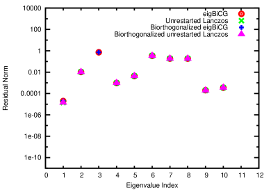
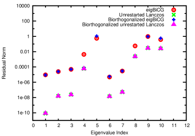
Figure 7: Comparing eigenvalue residual norms obtained with eigBiCG and benchmark algorithms for the QCD–49K (left) and QCD–249K (right) matrices.

Figure 8 shows the convergence history of the eigBiCG for the five smallest eigenvalues of the matrix light_in_tissue. Although not shown, the eigenvalue convergence history of the unrestarted Bi-Lanczos is identical. The right part of the figure plots $1-\|W^{(m)\dagger}V^{(m)}\|$ as a measure of the loss of biorthogonality between left and right basis vectors. As expected, this increases as the smallest eigenvalue converges.

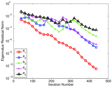
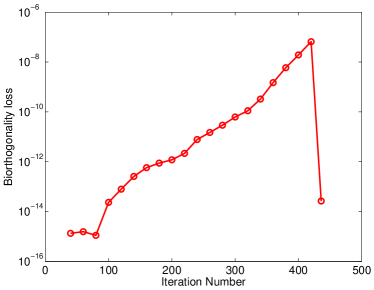
Figure 8: eigBiCG(10,40) on the light_in_tissue matrix. Left: convergence history of the five smallest eigenvalues. Right: Loss of biorthogonality between $V^{(m)},W^{(m)}$.

5.4.2 Choosing $m$ and $k$ for eigBiCG.

Beyond the condition $m>2k$, the parameters $m,k$ should be chosen to minimize the computational cost and approximate well as many eigenvalues as possible. As we discussed earlier, eigBiCG is stopped when the linear system converges so interior eigenvalues are not expected to be as accurate as the smallest one. Therefore, choosing $k$ large in order to approximate more eigenvalues has diminishing returns while increasing computational cost as $O(k^{2})$. On the other hand, the $2k$ vectors should encapsulate the information of the whole $V^{(m)}$ subspace at restart, so choosing $k$ too small deteriorates eigenvalue convergence. In our experiments we have observed that values of $k$ between 10 and 15 yield the best results. Given a reasonable choice for $k$, we have observed that the accuracy of the eigenvectors is not very sensitive to the value of $m$, so there is no reason to increase $m$ too much. A typical choice such as $2k+10$ or $2k+20$ was found to be sufficient. An exploration of the effect of various choices of $m,k$ for the QCD matrices is shown in Figures 9 and 10. These results are typical of other matrices as well. A further fine-tuning of $m,k$ is also problem dependent, based on the conditioning of the matrix (as deflation benefits may be limited) and the number of right-hand sides.

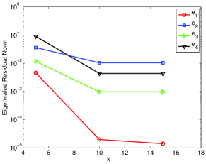
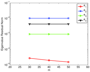
Figure 9: QCD–49K matrix: Residual norms of 4 smallest eigenvalues. Left: from eigBiCG(k,40) as a function of $k$. Right: from eigBiCG(10,m) as a function of $m$.

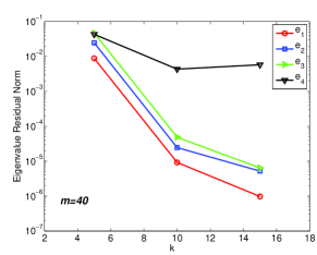
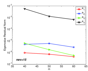
Figure 10: QCD–249K matrix: Residual norms of 4 smallest eigenvalues. Left: from eigBiCG(k,40) as a function of $k$. Right: from eigBiCG(15,m) as a function of $m$.

5.5 Experiments with Incremental eigBiCG

We generated 21 random right-hand sides $b_{i}$. The first 20 systems are solved using eigBiCG and the 21st system is solved using init-BiCGStab that is deflated by the accumulated approximate eigenspace. The 21st system is also solved using undeflated BiCGStab for comparison.

In Figure 11, we show the convergence of the residual norm of every third linear system in phase one and for the 21st system (phase two) for matrices $light\_in\_tissue$ and $PD$. We use $tol=10^{-10}$, $m=40$, $k=10$, and $btol=10^{-4}$. We observe faster convergence as we solve more systems and deflate with more and better quality eigenvectors. During the first phase, i.e. solving the first 20 systems using eigBiCG, the residual norm drops faster up to a certain value and then convergence slows down. As we discussed earlier, when the linear system residual converges to a tolerance comparable to the accuracy of the eigenvectors, the iteration “sees” again the eigenvectors and deflation effects cease. As more systems are solved, the eigenvectors improve incrementally, and thus the slow down occurs at lower tolerances. If we restart and deflate again, we obtain faster convergence as we see for the 21st system with init-BiCGStab.

In Figure 12, we show the number of matrix-vector multiplications used to reach convergence for the 21 systems solved. We also show results for undeflated BiCG and BiCGStab, which are respectively 5 and 2.5 times slower than our method.

In Figure 13, we compare the speedup obtained for solving the 21st system with init-BiCGStab when deflating with different numbers of approximate eigenvectors. For these problems, a modest number of eigenvectors provide the most part of speedup. In general, this would depend on the distribution and clustering of the eigenvalues. In the results shown above, init-BiCGStab was restarted only once when the system converged to $rtol=10^{-8}$.

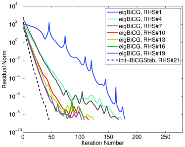
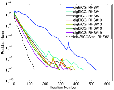
Figure 11: Convergence of some of the linear systems solved using eigBiCG and $init-$BiCGStab for the matrix $PD$(left) and $light\_in\_tissue$(right). The first 20 systems are solved using eigBiCG (40,10), and the 21st system is solved using init-BiCGStab deflated with 200 eigenvectors.

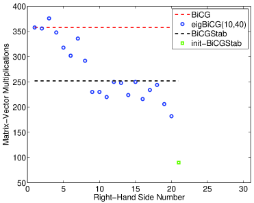
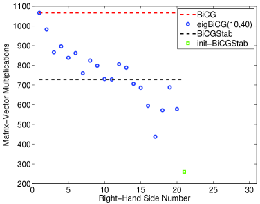
Figure 12: Reduction of the number of matrix-vector multiplications as we solve more systems for the matrix $PD$(left) and $light\_in\_tissue$(right). For comparison, we also show the number of matrix-vector multiplications using standard BiCG and BiCGStab.

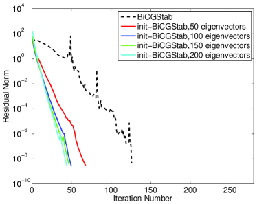
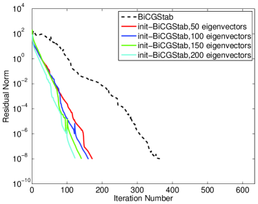
Figure 13: Effect of increasing the number of eigenvectors deflated on the number of iterations used by init-BiCGStab for the matrices $PD$(left) and $light\_in\_tissue$(right). The plot shows that a small number of eigenvectors was enough to give the bulk of speedup.

We next show results for the QCD matrices. For these tests we used $m=40,$ $k=15$, $tol=10^{-10}$, and $btol=10^{-4}$. init-BiCGStab was only restarted once when the linear system converged to a tolerance of $10^{-8}$. In Figure 14, we compare BiCGStab to init-BiCGStab where the number of deflated eigenvectors is obtained from different numbers of right hand sides. Overall, just a few eigenvectors yield a speedup of two or more. To illustrate the improvement of the eigenvectors as we solve more systems, we show in Figure 15 the residual norm for the best 50 eigenvalues computed and how this improves over time.

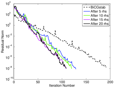
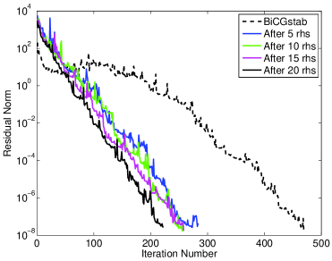
Figure 14: Convergence of undeflated BiCGStab versus $init-$BiCGStab deflated with the eigenvectors obtained after solving a different number of systems, for the matrices $QCD-49K$(left) and $QCD-249K$(right). A small number of eigenvectors is enough to give most of the speedup.

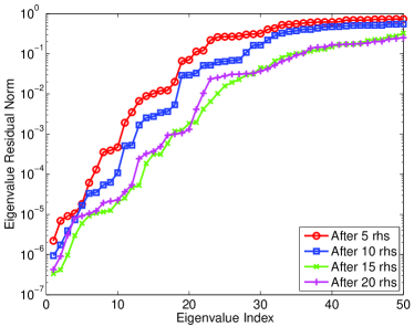
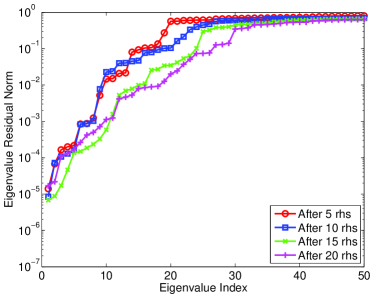
Figure 15: Improvement of the accuracy of the best 50 eigenvalues computed with Incremental eigBiCG(15,40) as more systems are solved for the matrices $QCD-49K$(left) and $QCD-249K$(right).

We conclude this subsection by observing that in all our previous experiments, a single restart of the deflated init-BiCGStab gave the best convergence. Therefore, as long as the vectors can be stored, the computational cost of applying the deflation projector is negligible (in QCD problems one matrix-vector operation costs about the same as an application of a projector with 300 vectors).

5.6 Comparing with GMRes–DR/GMRes–Proj

The GMRes-DR(m,k) algorithm [17] solves a nonsymmetric linear system using restarted GMRes and simultaneously computes $k$ approximate eigenvectors. Like eigBiCG, it uses a subspace of maximum size $m$ which is restarted to update $k$ approximations to the desired eigenvectors. Unlike eigBiCG, however, it explicitly orthogonalizes future iterates to these $k$ eigenvector approximations, thus improving also the convergence of the restarted GMRes(m). In theory, the advantages of eigBiCG are that (a) the biorthogonality of the whole space is implicit, (b) it uses not only thick but also locally optimal restarting to update the $k$ eigenvectors, (c) the underlying Krylov method is unrestarted, and (d) produces both left and right eigenvectors. The advantage of GMRes-DR(m,k) is that it is equivalent to the IRA eigensolver [27]. In practice, the most important difference is the performance of the underlying methods (GMRes(m), BiCG ) on a particular problem.

For systems with multiple right-hand sides, the computed eigenvectors from the first system are used to deflate Restarted GMRes for the following systems. Because it is expensive to deflate these $k$ vectors at every step of GMRes-DR(m,k), they are used in the GMRes-Proj method [38]. In GMRes-Proj, cycles of GMRes($m^{\prime}$) are alternated with a minimum residual projection over these $k$ eigenvectors. To maintain the same memory cost, usually $m^{\prime}=m-k$. Therefore, GMRes-Proj applies deflation only periodically, like our restarted init-BiCGStab. The difference is that GMRes-Proj applies the projection every $m^{\prime}$ steps and thus the total number of projections depends on the convergence rate of the problem, while init-BiCGStab is restarted a constant number of times, $tol/rtol$. Moreover, all eigenspace information comes from one run of GMRes-DR(m,k), while Incremental eigBiCG builds the eigenspace by accumulating vectors from $n_{1}$ right-hand sides.

A thorough comparison between Incremental eigBiCG and GMRes–DR/GMRes-Proj requires experimentation on a large parametric space, with different objectives (time, memory, iterations), and application problems. This is beyond the scope of this paper. Instead, we provide a sample experiment that shows that our method is competitive to a state-of-the-art method for solving systems with multiple right-hand sides. We use the two QCD matrices from our previous experiments and report also timings because the methods have different costs per iteration.

We solve linear systems for 100 random right-hand sides to $||r||<10^{-10}||b||$. After solving the first system with GMRes–DR(80,60), we obtain 60 (approximate) eigenvectors which we deflate at every cycle of GMRes(20)-Proj(60) for the next 99 systems. For Incremental eigBiCG, we solve the first 5 systems using eigBiCG(12,40) accumulating 60 left and right eigenvectors. These are then used to deflate init-BiCGStab without restarting for the rest 95 systems. To match the memory used by Incremental eigBiCG, we also compare against GMRes–DR(140,120) followed by GMRes(20)–Proj(120). The large subspace makes the latter method more expensive per step but it should have better deflation properties.

In Figure 16, we compare the residual norms of the best 60 eigenvectors computed by each of the three methods. We mention that the eigenvalues of the QCD matrices are symmetrically located around 0 which does not favor Bi-Lanczos. As an exact eigensolver with a large subspace (80 or 140 vectors) GMRes-DR produces better residual norms than Incremental eigBiCG.

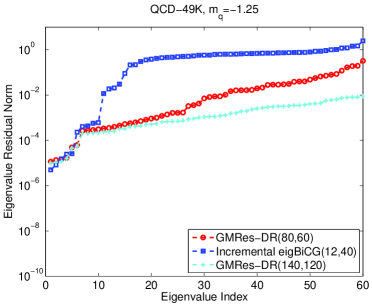
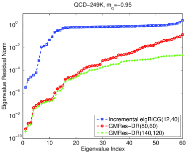
Figure 16: Residual norms of the lowest 60 eigenvalues of the QCD matrices computed using GMRes–DR(60,80), GMRes–DR(120,140), and Incremental eigBiCG(12,40) for 5 right-hand sides.

Figure 17 shows the cost for solving each of the 100 systems for QCD–49K. For the first system the number of iterations is similar for all methods, but BiCG requires two matrix-vector products per iteration. For subsequent deflated systems, BiCGStab required only a few more products than the GMRES–Proj variants. The right part of the figure shows that the inexpensive deflation and iteration step of init-BiCGStab make it faster than GMRES–Proj, especially when a large number of right-hand sides need to be solved. The only exception is the short incremental phase where BiCG is used which converges slower than BiCGStab.

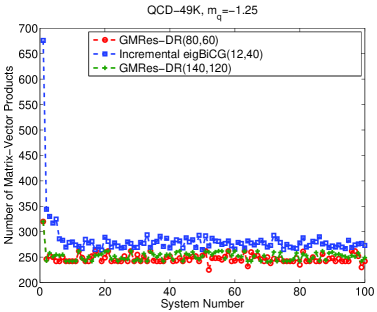
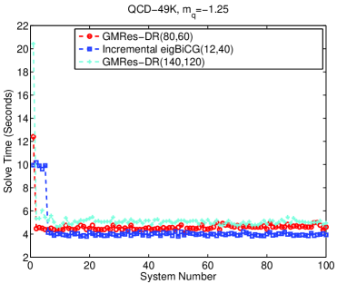
Figure 17: Solving 100 right-hand sides using GMRES–DR(m,k) and Incremental eigBiCG(nev,m) for the QCD–49K matrix. The first system is solved with GMRES–DR(m,k) and the subsequent 99 systems are solved using GMRES(m-k)–Proj(k) in which k eigenvectors are deflated. For Incremental eigBiCG(nev,m), the first 5 systems are solved with eigBiCG(nev,m) and the subsequent 95 systems with init-BiCGStab with 5*nev eigenvectors deflated. On the left, we show the number of matrix-vector products in both cases. On the right we show the solution time. For this problem, Incremental eigBiCG is faster than GMRES–DR.

Figure 18 shows similar results for the matrix QCD–249K. init-BiCGStab took about 50% more matrix-vector products than GMRes-DR (although the number of iterations was smaller) but all methods achieved solutions in similar times.

We note that the parameter choices for Incremental eigBiCG were not the best ones identified in previous sections because we wanted all methods to use either the same number of deflation vectors or the same memory. With the best parameters, the number of matrix-vector products of Incremental eigBiCG is less than that of GMRES–Proj for QCD–49K and about the same for QCD–249K (see Figure 14) and thus we expect our method to be quite faster.

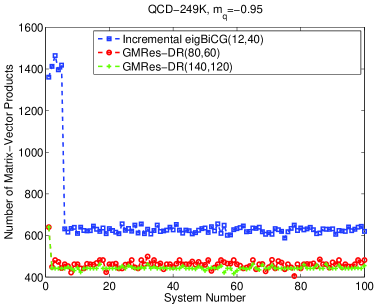
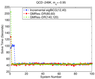
Figure 18: Solving 100 right-hand sides using GMRES–DR(m,k) and Incremental eigBiCG(nev,m) for the QCD–249K matrix. The procedure and parameters are the same as in Figure 17. On the right we show the solution time. For this problem, Incremental eigBiCG is equally fast to GMRES–DR.

6 Conclusions

We have extended the eigCG algorithm for solving linear systems with multiple right-hand sides to the nonsymmetric case. The resulting algorithm, eigBiCG, approximates a few smallest magnitude eigenvalues and their corresponding left and right eigenvectors while a linear system is solved with BiCG. The algorithm uses only a small size window of the BiCG residuals without affecting the convergence of the linear system and without restarting BiCG. The eigBiCG algorithm was tested on matrices from different applications. For nonsymmetric, non-defective matrices with a positive definite symmetric part, eigBiCG was able to compute eigenvalues almost as accurately as those computed with unrestarted and even explicitly biorthogonalized Bi-Lanczos algorithms.

For systems with multiple right-hand sides, we have given an algorithm that incrementally improves the number and accuracy of the eigenvalues computed with eigBiCG while solving the first few systems. The computed eigenvectors are then used to deflate BiCGStab not at every step, but only initially at the right-hand side. Repeating this deflation once or twice by restarting BiCGStab was always sufficient. In our experiments our deflated method achieved speedups of a factor of two or more. We also showed that the method is competitive to a state-of-the-art method for multiple right-hand sides, the GMRes-DR/GMRes-Proj.

Further improvements of the algorithms that are also relevant for the SPD case could be investigated in the future. Examples include, how to implement selective biorthogonalization to reduce the effect of biorthogonality loss in eigBiCG, how to reduce the number of accumulated vectors in Incremental eigBiCG by restarting the bases, or what the effect of deflation is on the accuracy of the solution of the linear system.

This work was supported by the National Science Foundation grant CCF-0728915, the DOE Jefferson Lab, the Jeffress Memorial Trust grant J-813, and received partial support through the Scientific Discovery through Advanced Computing (SciDAC) program funded by U.S. Department of Energy, Office of Science, Advanced Scientific Computing Research and Nuclear Physics under award number DE-FC02-12ER41890. A. Abdel-Rehim was partially supported by the PRACE-2IP project (Partnership for Advanced Computing in Europe, Second Implementation Phase) under WP8 grant number EC-RI-283493.

References

- [1] Saad Y. Iterative Methods for Sparse Linear Systems. SIAM: Philadelphia, PA, USA, 2003.
- [2] Simoncini V, Szyld DB. Recent computational developments in Krylov subspace methods for linear systems. Numerical Linear Algebra with Appl. 2007; 14(1):1–59.
- [3] Gutknecht MH. Block Krylov space methods for linear systems with multiple right-hand sides: an introduction. Modern Mathematical Models, Methods and Algorithms for Real World Systems. Anamaya Publishers: New Delhi, India, 2006. Http://www.sam.math.ethz.ch/mhg.
- [4] Golub GH, Underwood R. The block Lanczos method for computing eigenvalues. Mathematical Software III, Rice JR (ed.). Academic Press, 1977; 361–377.
- [5] O’Leary DP. The block conjugate gradient algorithm and related methods. Lin. Alg. Appl. February 1980; 29:293–322.
- [6] Guennouni AE, Jbilou K, Sadok H. The block Lanczos method for linear systems with multiple right hand sides. Appl. Numer. Math. 2004; 51(2–3):243–256.
- [7] Freund RW, Malhotra M. A block QMR algorithm for non-Hermitian linear systems with multiple right-hand sides. Linear Algebra and its Applications 1997; 254(1–3):119–157.
- [8] Vital B. Etude de quelques mthodes de rsolution de problmes linaires de grande taille sur multiprocesseur. PhD Thesis, Universit de Rennes, Rennes, France 1990.
- [9] Guennouni AE, Jbilou K. Block and seed BiCGStab algorithms for nonsymmetric multiple linear systems 2000. Http://citeseerx.ist.psu.edu/viewdoc/summary?doi=10.1.1.11.6249.
- [10] Guennouni AE, Jbilou K, Sadok H. A block version of BiCGStab for linear systems with multiple right-hand sides. Electronic Transactions on Numerical Analysis 2003; 16:129–142.
- [11] Smith CF. The performance of preconditioned iterative methods in computational electromagnetics. PhD Thesis, University of Illinois at Urbana-Champaign, Urbana, IL 1987.
- [12] Smith C, Peterson A, Mittra R. A conjugate gradient algorithm for the treatment of multiple incident electromagnetic fields. IEEE Trans. Antennas and Propagation 1989; 37:1490––1493.
- [13] Simoncini V, Gallopoulos E. An iterative method for nonsymmetric systems with multiple right hand sides. SIAM J. Sci. Comput. 1995; 16(4):917–933.
- [14] Chan TF, Wan WL. Analysis of projection methods for solving linear systems with multiple right hand sides. SIAM J. Sci. Comput. 1997; 18:1698–1721.
- [15] Saad Y. On the Lanczos method for solving symmetric linear systems with several right hand sides. Math. Comp. 1987; 48:651–662.
- [16] Saad Y, Yeung M, Erhel J, Guyomarc’h F. A deflated version of the conjugate gradient algorithm. SIAM J. Sci. Comput. 2000; 21(5):1909–1926.
- [17] Morgan RB. GMRES with deflated restarting. SIAM J. Sci. Comput. 2002; 24:20–37.
- [18] Wang S, de Sturler E, Paulino GH. Large-scale topology optimization using preconditioned Krylov subspace methods with recycling. International Journal for Numerical Methods in Engineering 2007; 69(12):2441–2468.
- [19] Ahuja K, de Sturler E, Chang ER, Gugercin S. Recycling bicg for model reduction 2010. ArXiv:1010.0762v1 [http://arxiv.org/abs/1010.0762].
- [20] Wu K, Simon H. Thick-restart Lanczos method for large symmetric eigenvalue problems. SIAM J. Matrix Anal. Appl. 2000; 22(2):602–616.
- [21] Stathopoulos A, Saad Y, Wu K. Dynamic thick restarting of the Davidson, and the implicitly restarted arnoldi methods. SIAM J. Sci. Comput. 1998; 19(1):227–245.
- [22] Stathopoulos A, Orginos K. Computing and deflating eigenvalues while solving multiple right-hand side linear systems with an application to quantum chromodynamics. SIAM J. Sci. Comput. 2010; 32(1):439–462.
- [23] Abdel-Rehim AM, Morgan RB, Nicely DA, Wilcox W. Deflated and restarted symmetric lanczos methods for eigenvalues and linear equations with multiple right-hand sides. SIAM J. Sci. Comput. 2010; 32:129–149.
- [24] D Darnell RBM, Wilcox W. Deflated GMRES for systems with multiple shifts and multiple right-hand sides. Linear Algebra and its Applications 2008; 429:2415–2434.
- [25] Morgan RB. Restarted block-GMRES with deflation of eigenvalues. Applied Numerical Mathematics 2005; 54:222–236.
- [26] Kilmer M, Miller E, Rappaport C. QMR-based projection techniques for the solution of non-hermitian systems with multiple right-hand sides. SIAM Journal on Scientific Computing 2002; 23(3):761–780.
- [27] Lehoucq RB, Sorensen DC, Yang C. ARPACK User’s Guide: Solution of Large-Scale Eigenvalue Problems with Implicitly Restarted Arnoldi Methods. SIAM, Philadelphia, PA, USA 1998.
- [28] Stathopoulos A, McCombs JR. PRIMME: PReconditioned Iterative Multimethod Eigensolver: Methods and software description. ACM Transaction on Mathematical Software 2010; 37(2):21:1–21:30.
- [29] Stathopoulos A. Nearly optimal preconditioned methods for Hermitian eigenproblems under limited memory. Part I: Seeking one eigenvalue. SIAM J. Sci. Comput. 2007; 29:481–514.
- [30] Stathopoulos A, McCombs JR. Nearly optimal preconditioned methods for Hermitian eigenproblems under limited memory. Part II: Seeking many eigenvalues. SIAM J. Sci. Comput. 2007; 29:2162–2188.
- [31] Knyazev AV. Toward the optimal preconditioned eigensolver: Locally optimal block preconditioned conjugate gradient method. SIAM J. Sci. Comput. 2001; 23(2):517–541.
- [32] de Sturler E. Truncation strategies for optimal Krylov subspace methods 1999; 36:864–889.
- [33] Baker A, Jessup E, Manteuffel T. A technique for accelerating the convergence of restarted gmres. SIAM Journal on Matrix Analysis and Applications 2005; 26:962–984.
- [34] Stathopoulos A. A case for a biorthogonal Jacobi-Davidson method: restarting and correction equation. SIAM Journal on Matrix Analysis and Applications 2002; 24(1):238–259.
- [35] Frank J, Vuik C. On the construction of deflation-based preconditioners. SIAM J. Sci. Comput. 2001; 23:442.
- [36] Rendel O, Jens-Peter M Z. Tuning IDR to fit your applications. Proceedings of a Workshop at Doshisha University, 2011. Http://www.tu-harburg.de/matjz/papers/.
- [37] Morgan RB, Nicely DA. Restarting the nonsymmetric Lanczos algorithm for eigenvalues and linear equations including multiple right-hand sides. SIAM J. Sci. Comput. 2011; 33:3037–3056.
- [38] Morgan RB, Wilcox W. Deflated iterative methods for linear equations with multiple right-hand sides. Technical Report BU-HEPP-04-01, Baylor University 2004. ArXiv:math-ph/0405053.
- [39] Brandt A. Multi-level adaptive solutions to boundary-value problems. Mathematics of Computation 1977; 31(138):333–390.
- [40] Luscher M. Local coherence and deflation of the low quark modes in Lattice QCD. JHEP 2007; 0707:081. ArXiv:0706.2298[hep-lat].
- [41] Babich R, Brannick J, Brower RC, Clark MA, Manteuffel TA, McCormick SF, Osborn JC, Rebbi C. Adaptive multigrid algorithm for the lattice Wilson-Dirac operator. Phys. Rev. Lett. 2010; 105:201 602, 10.1103/PhysRevLett.105.201602.
- [42] D’yakonov EG. Iteration methods in eigenvalue problems. Math. Notes 1983; 34:945–953.
- [43] Knyazev AV. Convergence rate estimates for iterative methods for symmetric eigenvalue problems and its implementation in a subspace. International Ser. Numerical Mathematics 1991; 96:143–154. Eigenwertaufgaben in Natur- und Ingenieurwissenschaften und ihre numerische Behandlung, Oberwolfach, 1990.
- [44] Murray CW, Racine SC, Davidson ER. Improved algorithms for the lowest eigenvalues and associated eigenvectors of large matrices. J. Comput. Phys. 1992; 103(2):382–389.
- [45] Stathopoulos A, Saad Y. Restarting techniques for (Jacobi-)Davidson symmetric eigenvalue methods. Electr. Trans. Numer. Anal. 1998; 7:163–181.
- [46] Lanczos C. Solution of systems of linear equations by minimized iterations. J. Res. Nat. Nur. Stand. 1952; 49:33–53.
- [47] Fletcher R. Conjugate gradient methods for indefinite systems. Lecture Notes in Mathematics, vol. 506. Springer-Verlag: Berlin-Heidelberg-New York, 1976; 73–89.
- [48] Tong CH, Ye Q. Analysis of the finite precision Bi-Conjugate Gradient algorithm for nonsymmetric linear systems. Math. Comp. Oct 2000; 69(232):1559–1575.
- [49] Bai Z. Error analysis of the lanczos algorithm for the nonsymmetric eigenvalue problem. Math. Comp. 1994; 65:209–226.
- [50] Taylor DR. Analysis of the look ahead Lanczos algorithm. PhD Thesis, University of California, Berkeley 1982.
- [51] Parlett BN, Taylor DR, Liu ZA. A look ahead Lanczos algorithm for unsymmetric matrices. Math. Comp. 1985; 44:105–124.
- [52] Freund RW, Gutknecht MH, Nachtigal NM. An implementation of the look ahead lanczos algorithm for non-hermitian matrices, Part I. Technical Report 90.45, RIACS, NASA Ames Research Center 1990.
- [53] Freund RW, Gutknecht MH, Nachtigal NM. An implementation of the look ahead lanczos algorithm for non-hermitian matrices, Part II. Technical Report 90.45, RIACS, NASA Ames Research Center 1990.
- [54] Saad Y. SPARSKIT: A basic tool-kit for sparse matrix computations. Http://www-users.cs.umn.edu/ saad/software/SPARSKIT/sparskit.html.
- [55] Davis T. The university of florida sparse matrix collection. http://www.cise.ufl.edu/research/sparse/matrices/index.html.
- [56] Rothe HJ. Lattice Gauge Theories: An introduction. World Scientific Publishing Co. Pte. Ltd., 2005.
- [57] Gupta R. Introduction to Lattice QCD 1998. ArXiv:hep-lat/9807028v1 [http://arxiv.org/abs/hep-lat/9807028].
- [58] Muta T. Foundations of Quantum Chromodynamics, An Introduction to Perturbative Methods in Gauge Theories. World Scientific Publishing Co. Pte. Ltd., 1987.
- [59] Donoghue J, Golowich E, Holstein BR. Dynamics of the Standard Model. Cambridge University Press, 1992.
- [60] Gsken S. Flavor singlet phenomena in Lattice QCD. ArXiv:hep-lat/9906034.
- [61] Wilcox W. Noise methods for flavor singlet quantities 1999. ArXiv:hep-lat/9911013v2.
- [62] Bali GS, Collins S, Schaefer A. Effective noise reduction techniques for disconnected loops in Lattice QCD. Computer Physics Communications 2010; 181:1570–1583.