Effect of noise on generalized synchronization of chaos: theory and experiment

Abstract

The influence of noise on the generalized synchronization regime in the chaotic systems with dissipative coupling is considered. If attractors of the drive and response systems have an infinitely large basin of attraction, generalized synchronization is shown to possess a great stability with respect to noise. The reasons of the revealed particularity are explained by means of the modified system approach [A. E. Hramov, A. A. Koronovskii, Phys. Rev. E. 71, 067201 (2005)] and confirmed by the results of numerical calculations and experimental studies. The main results are illustrated using the examples of unidirectionally coupled chaotic oscillators and discrete maps as well as spatially extended dynamical systems. Different types of the model noise are analyzed. Possible applications of the revealed particularity are briefly discussed.

Introduction

Synchronization is one of the most relevant directions of nonlinear dynamics attracting great attention of modern scientists Pikovsky:2002_SynhroBook ; Boccaletti:2002_ChaosSynchro . The interest to it is connected both with a large fundamental significance of its investigation Pikovsky:2002_SynhroBook and a wide practical applications, e.g. for the transmission of information Roy:Chaos_Nature2005 ; Jaeger:Science2004ChaosComm ; Parlitz:1992_ChaoticCommunication ; Cuomo:1993_ChaosCommunication ; Kocarev:1995_ChaoticComunication ; Peng:1996_GyperChaosSynchro ; Eguia:2000 ; Fischer:2000_ChaosCommunication ; Rulkov:2002_ChaoticCommunication ; Yuan_SecureCommunication:2005 ; Li_ChaoticTrans:2006 ; Fradkov_ChaosTrans:2006 ; Cessac:TransSign2006 ; Rohde:EstSecCom2008 ; Materassi:TimeScalingSecure:2008 ; alkor:2010_SecureCommunicationUFNeng , diagnostics of dynamics of some biological systems Strogatz:1994_ChaosBook ; Elson:1998_NeronSynchro ; Porcher:2001_LEinMedicine ; Glass:2001_SynchroBio ; Pavlov:MultiscalityPhysA2002 ; Rosenblum:2004_SynchroBioSystems , control of chaos in the microwave systems Ditto:1990_ControllingChaos ; Ticos:2000_PlasmaDischarge ; Rosa:2000_PlasmaDischarge ; Hramov:2005_Chaos_BWO ; dmitriev:074101 , etc.

Several types of the synchronous chaotic system behavior are traditionally distinguished. They are phase Rosenblum:1996_PhaseSynchro ; Pikovsky:2002_SynhroBook , generalized Rulkov:1995_GeneralSynchro ; Kocarev:1996_GS , lag Rosenblum:1997_LagSynchro ; Taherion:1999_LagSynchro , complete Pecora:1990_ChaosSynchro ; Pecora:1991_ChaosSynchro , time scale Hramov:2004_Chaos ; Aeh:2005_TSS:PhysicaD ; Hramov:2005_Chaos_BWO synchronization and others.

One of the most important problems connected with the study of the chaotic systems is the influence of noise on their behavior including the synchronous regime arising Stone:726 ; Kifer:StochMathJ1981 ; Ali:1997_NoiseSynchro ; Toral:2001_NoiseSynchro ; Anishchenko:2002_SynchroEng ; Zhou:PRL2002 ; Zhou:2002_NoiseEnhancedPS ; Kuznetsov:2003_WeakSynchroAndNoise ; Zhou:PRE2003 ; Goldobin:2005_SynchroCommonNoise ; Hramov:2006_PLA_NIS_GS ; Guan:NoiseGS:2006 . Noise is known to influence on system dynamics in different ways. In particular, in case of complete synchronization of coupled chaotic oscillators, noise may induce intermittent loss of synchronization due to local instability of the synchronization manifold Heagy:CSNoise_PRE1995 ; Gauthier:PRL1996_CSNoise . At the same time, both periodic and chaotic non-coupled identical dynamical systems subjected to a common noise may achieve complete synchronization at a large enough intensity Fahy:1992_NoiseInfluence ; Martian:1994_SynchroNoise ; Jensen:1998NISPeriodic ; Toral:2001_NoiseSynchro ; Goldobin:2005_SynchroCommonNoise . Such phenomenon is called noise-induced synchronization regime. In the case of phase synchronization of coupled oscillators noise can induce phase slips in phase-locked periodic and chaotic oscillators Zhu:2001_transient ; Hramov:2007_TypeIAndNoise . On the other hand, noise can play a constructive role at phase synchronization enhancing the synchronous regime below the threshold of phase synchronization Zhou:2002_NoiseEnhancedPS ; Hramov:ZeroLE_PRE2008 . Nevertheless, for almost all types of chaotic synchronization (phase synchronization, complete synchronization, lag synchronization) noise appears to obstruct the synchronous motion and increase the value of the coupling strength between oscillators corresponding to the onset of synchronization.

At the same time, effect of noise on the generalized synchronization regime is investigated poorly enough. As an exception one can refer to the paper Guan:NoiseGS:2006 where the effect of noise on generalized synchronization in two characteristically different chaotic oscillators have been considered. In this case the effect of noise can be system dependent, i.e. common noise can either induce/enhance or destroy the generalized synchronization regime.

Systems studied in Guan:NoiseGS:2006 are close to an attractor crisis bifurcation Grebogi:1982_crisis . In this case external noise of small intensity may result in creation of a new chaotic attractor with a qualitatively different topology that results in changing of the system behavior in the presence of noise. In present paper we dwell for the first time upon the behavior of the generalized synchronization regime in systems which attractors are far away from the boundary bifurcation crisis or their basins of attraction are infinitely large. We report for the first time theoretical and experimental results of the influence of noise on the threshold of the generalized synchronization regime in identical systems with mismatched parameters whose attractors satisfy the conditions mentioned above. As it would be shown bellow, in this case the generalized synchronization onset is almost independent on the noise intensity, i.e. the synchronous regime appears in the absence and presence of noise practically for the same values of the coupling parameter strength. At the same time, if the system attractors are far away from the boundary bifurcation crisis, with their basins of attraction being limited, the stability of the generalized synchronization regime with respect to external noise would be observed in the large, but limited range of the noise intensity. The same findings also remain to be correct for the systems with the infinitely large basin of attraction, although the causes of such type of behavior are different.

Revealed peculiarity of the behavior of the boundary of the GS regime in the presence of noise could be used in many relevant circumstances, e.g. for the secure transmission of information through the communication channel alkor:2010_SecureCommunicationUFNeng ; Moskalenko:InfoTransNoisePLA2010 , in the medical, physiological Hramov:2006_Prosachivanie ; Hramov:2007_UnivariateDataPRE and other practical applications where the level of natural noise is sufficient.

The structure of the paper is as follows. Section 1 contains brief description of the generalized synchronization regime, its methods for detection and mechanisms of its arising both in the cases of the absence and presence of noise. The reasons of the stability of the generalized synchronization regime with respect to noise are also discussed in this section. Section 2 presents results of numerical simulation of the influence of noise on the threshold of the synchronous regime arising in several systems with discrete and continuous time as well as spatially extended systems demonstrating spatio-temporal chaos. In Section 3 we describe the experimental setup for the observation of the generalized synchronization regime in the presence of noise in the electronic chaotic circuit and give the results obtained by means of it. Final discussions and remarks are given in Conclusions.

1 Generalized synchronization regime

The generalized synchronization regime (GS) in two unidirectionally coupled chaotic oscillators with continuous

$$\begin{split}&\mathbf{\dot{x}}(t)=\mathbf{G}(\mathbf{x}(t),\mathbf{g}_{d})\\ &\mathbf{\dot{u}}(t)=\mathbf{H}(\mathbf{u}(t),\mathbf{g}_{r})+\varepsilon\mathbf{P}(\mathbf{x}(t),\mathbf{u}(t)),\\ \end{split}$$ (1)

or discrete

$$\begin{split}&\mathbf{x}_{n+1}=\mathbf{G}(\mathbf{x}_{n},\mathbf{g}_{d})\\ &\mathbf{u}_{n+1}=\mathbf{H}(\mathbf{u}_{n},\mathbf{g}_{r})+\varepsilon\mathbf{P}(\mathbf{x}_{n},\mathbf{u}_{n}),\\ \end{split}$$ (2)

time means the presence of a functional relation

$${\mathbf{u}=\mathbf{F}[\mathbf{x}]}$$ (3)

between the drive $\mathbf{x}$ ($\mathbf{x}(t)$ or $\mathbf{x}_{n}$) and response $\mathbf{u}$ ($\mathbf{u}(t)$ or $\mathbf{u}_{n}$) system states Rulkov:1995_GeneralSynchro ; Pyragas:1996_WeakAndStrongSynchro , i.e. in the GS regime the response system behavior converges to the synchronized state independently on the choice of initial conditions belonging to the same basin of attraction. In equations (1)–(2) $\mathbf{x}$ and $\mathbf{u}$ are the state vectors of the drive and response systems, respectively; $\mathbf{G}$ and $\mathbf{H}$ define the vector fields of interacting systems, $\mathbf{g}_{d}$ and $\mathbf{g}_{r}$ are the control parameter vectors, $\mathbf{P}$ denotes the coupling term, and $\varepsilon$ is the scalar coupling parameter. Typically, the analytical form of the relation $\mathbf{F}[\cdot]$ in (3) can not be found in most cases. Depending on the character of this relation – smooth or fractal – GS can be divided into the strong and the weak ones Pyragas:1996_WeakAndStrongSynchro , respectively. It is also important to note that the distinct dynamical systems (including the systems with the different dimension of the phase space) may be used as the drive and response oscillators to achieve the GS regime.

To detect the GS regime both in flow systems and discrete maps the auxiliary system method Rulkov:1996_AuxiliarySystem is frequently used. According to this method the behavior of the response system $\mathbf{u}$ is considered together with the auxiliary system $\mathbf{v}$ ($\mathbf{v}(t)$ in the case of the flow systems and $\mathbf{v}_{n}$ if maps are considered). The auxiliary system is equivalent to the response one by the control parameter values, but starts with other initial conditions belonging to the same basin of chaotic attractor (if there is the multistability in the system). If GS takes place, the system states $\mathbf{u}$ and $\mathbf{v}$ become identical after the transient is finished due to the existence of the relations $\mathbf{u}=\mathbf{F}[\mathbf{x}]$ and $\mathbf{v}=\mathbf{F}[\mathbf{x}]$. Thus, the coincidence of the state vectors of the response and auxiliary systems $\mathbf{v}\equiv\mathbf{u}$ is considered as a criterion of the GS regime presence.

It is also possible to compute the conditional Lyapunov exponents to detect the presence of GS Pyragas:1996_WeakAndStrongSynchro . In this case Lyapunov exponents are calculated for the response system, and since the behavior of this system depends on the drive system these Lyapunov exponents are called conditional. Negativity of the largest conditional Lyapunov exponent is a criterion of the GS presence in unidirectionally coupled dynamical systems Pyragas:1996_WeakAndStrongSynchro .

Methods for the GS regime detection described above could be easily applied for the investigation of the influence of noise on the GS regime onset, with all criteria of the GS regime appearance remaining unchangeable. In other words, the auxiliary system method and the conditional Lyapunov exponent calculation may be used to detect the existence of this type of synchronization both in flow systems and discrete maps in the presence of noise.

At the same time, taking into account the fact that the definition of the GS regime and methods for its detection are the same both for systems with continuous and discrete time, further in this Section we consider the GS regime onset in flow systems. Several peculiarities connected with the GS regime onset in discrete maps will be discussed in Section 2.1.

GS is known to take place in systems with the different types of coupling, the dissipative and non-dissipative ones. In the case of dissipatively coupled identical flow dynamical systems with mismatched parameters equations (1) can be rewritten as

$$\begin{split}&\mathbf{\dot{x}}(t)=\mathbf{H}(\mathbf{x}(t),\mathbf{g}_{d})\\ &\mathbf{\dot{u}}(t)=\mathbf{H}(\mathbf{u}(t),\mathbf{g}_{r})+\varepsilon\mathbf{A}(\mathbf{x}(t)-\mathbf{u}(t)),\end{split}$$ (4)

where $\mathbf{A}={\{\delta_{ij}\}}$ is the coupling matrix, $\delta_{ii}=0$ or $\delta_{ii}=1$, $\delta_{ij}=0$ ($i\neq j$). The mechanisms of the GS regime arising in systems with the dissipative coupling can be revealed by the modified system approach firstly proposed in our previous work Aeh:2005_GS:ModifiedSystem . Due to such approach the dynamics of the response system may be considered as the non-autonomous dynamics of the modified system

$$\mathbf{\dot{u}}_{m}(t)=\mathbf{H}^{\prime}(\mathbf{u}_{m}(t),\mathbf{g}_{r},\varepsilon)$$ (5)

where $\mathbf{H}^{\prime}(\mathbf{u}(t))=\mathbf{H}(\mathbf{u}(t))-\varepsilon\mathbf{A}\mathbf{u}(t)$, under the external force $\varepsilon\mathbf{A}\mathbf{x}(t)$:

$$\mathbf{\dot{u}}_{m}(t)=\mathbf{H}^{\prime}(\mathbf{u}_{m}(t),\mathbf{g}_{r},\varepsilon)+\varepsilon\mathbf{A}\mathbf{x}(t).$$ (6)

One can easily see that the term $-\varepsilon\mathbf{A}\mathbf{x}(t)$ brings the additional dissipation into the system (5). The phase flow contraction is characterized by means of the vector field divergence. Obviously, the vector field divergences of the modified and the response systems are related with each other as

$$\mathrm{div}\,\mathbf{H}^{\prime}=\mathrm{div}\,\mathbf{H}-\varepsilon\sum\limits_{i=1}^{N}\delta_{ii}$$ (7)

(where $N$ is the dimension of the modified system phase space), respectively. So, the dissipation in the modified system is greater than in the response one and it increases with the growth of the coupling strength $\varepsilon$.

The GS regime arising in (4) may be considered as a result of two cooperative processes taking place simultaneously. The first of them is the growth of the dissipation in the system (5) and the second one is an increase of the amplitude of the external signal. Both processes are correlated with each other by means of parameter $\varepsilon$ and can not be realized in the coupled oscillator system (4) independently. Nevertheless, it is clear, that an increase of the parameter $\varepsilon$ in the modified system (5) results in the simplification of its behavior and the transition from the chaotic oscillations to the periodic ones Aeh:2005_GS:ModifiedSystem . Moreover, if the additional dissipation is large enough the stable fixed state may be realized in the modified system. On the contrary, the external chaotic force $\varepsilon\mathbf{A}\mathbf{x}(t)$ tends to complicate the behavior of the modified system and impose its own dynamics on it. The GS regime is known to take place when own chaotic dynamics of the autonomous modified system is suppressed Aeh:2005_GS:ModifiedSystem . At the same time, the response system demonstrates chaotic oscillations due to the external signal coming from the drive system.

So, the stability of the GS regime is defined primarily by the properties of the modified system. Adding of noise does not change the characteristics of the modified system (5) and does not seem to affect the threshold of the GS regime onset. Therefore, the GS regime should exhibit the stability with respect to noise in the wide range of the noise intensities. At that, it should be noted that the characteristics of noise does not matter and the similar stability of the GS regime would be observed both for additive and multiplicative noise with different characteristics.

To verify the correctness of the statement mentioned above we use the conditional Lyapunov exponent method. We consider the evolution of both the reference state of the response oscillator $\mathbf{u}(t)$ and the perturbed one ${\mathbf{v}(t)=\mathbf{u}(t)+\mathbf{\Delta}(t)}$ being close to each other (i.e., $|\mathbf{\Delta}(t)|\ll 1$). The conditional Lyapunov exponents $\lambda_{i}^{r}$ ($i=1,\dots,N$) are determined by the exponential increase/decrease of the small perturbation $\mathbf{\Delta}(t)$. To take into account the noise influence we have added the noise terms $\zeta,\xi\in\mathbb{R}^{N}$ into equations (4) describing the dynamics of the drive and response systems:

$$\begin{split}&\mathbf{\dot{x}}(t)=\mathbf{H}(\mathbf{x}(t),\mathbf{g}_{d})+\mathbf{\zeta}(t)\\ &\mathbf{\dot{u}}(t)=\mathbf{H}(\mathbf{u}(t),\mathbf{g}_{r})+\varepsilon\mathbf{A}(\mathbf{x}(t)-\mathbf{u}(t))+\xi(t).\end{split}$$ (8)

In Eq. (8) the stochastic processes are supposed to be different for the more complicated case to be considered.

In this case the dynamics of the auxiliary (perturbed) system would be given by

$$\mathbf{\dot{v}}(t)=\mathbf{H}(\mathbf{v}(t),\mathbf{g}_{r})+\varepsilon\mathbf{A}(\mathbf{x}(t)-\mathbf{v}(t))+\xi(t).$$ (9)

Note, the concept of the generalized synchronization and the auxiliary system approach requires the identity of the signals driving both the response and auxiliary systems. This requirement means that noise must be also identical for the response and auxiliary system. In other words, the control parameter values and the noise signals in the response and auxiliary systems should be fully identical whereas initial conditions for them should be chosen different.

The equation determining the evolution of the perturbation $\mathbf{\Delta}(t)$ may be obtained as follows

$$\begin{array}[]{lll}\dot{\mathbf{\Delta}}(t)=\mathbf{H}(\mathbf{v}(t),\mathbf{g}_{r})-\mathbf{H}(\mathbf{u}(t),\mathbf{g}_{r})-\varepsilon A\mathbf{\Delta}(t).\end{array}$$ (10)

Taking into account that $\mathbf{v}(t)=\mathbf{u}(t)+\mathbf{\Delta}(t)$ and ${|\mathbf{\Delta}(t)|\ll 1}$, one can write

$$\mathbf{H}(\mathbf{v}(t),\mathbf{g}_{r})\approx\mathbf{H}(\mathbf{u}(t),\mathbf{g}_{r})+\mathbf{J}\mathbf{H}(\mathbf{u}(t),\mathbf{g}_{r})\mathbf{\Delta}(t)$$ (11)

(where $\mathbf{J}$ is a Jakobian matrix), and, as a consequence

$$\dot{\mathbf{\Delta}}(t)=(\mathbf{J}\mathbf{H}(\mathbf{u}(t))-\varepsilon\mathbf{A})\Delta(t)=\mathbf{J}\mathbf{H}^{\prime}(\mathbf{u}(t))\mathbf{\Delta}(t),$$ (12)

Eq. (12) is the variational equation for the computation of the conditional Lyapunov exponents of the response system describing by Eq. (8) as well as Eq. (4). Therefore, one can conclude that the largest conditional Lyapunov exponents (determining the threshold of the GS regime onset) would behave in the similar way both in the absence and presence of noise. Therefore, the threshold of GS should not considerably depend on the noise intensity, whereas the GS regime should exhibit the stability to the noise influence. Note, also, that the vector state ${\mathbf{u}(t)}$ in Eq. (12) depends on the noise signals, and, therefore, the largest conditional Lyapunov exponents obtained for the cases with and without noise are, however, not equivalent. As a consequence, the great intensities of noise may change the stability properties of the modified system that may result in the variation of the value of the threshold of the GS regime.

It should be noted that onset of the GS regime is similar to the last one for the cases of complete (CS) (identical) and lag (LS) synchronization. Such types of the synchronous chaotic system behavior could be considered as partial cases of GS and they correspond to the stronger forms of such regime Pyragas:1996_WeakAndStrongSynchro . It is clear that the modified system approach could be applied for revealing the mechanisms resulting in the synchronous regime onset even in the presence of noise. At the same time, it should be noted that even for identical dynamical systems with equal values of the control parameters GS regime arises a bit earlier than the CS one Pyragas:1996_WeakAndStrongSynchro ; Harmov:2005_GSOnset_EPL . As it would be shown bellow in Section 2.2, external noise added to the drive and response could destroy the CS (or LS) regime but it does not destruct the GS regime itself. Therefore, the stability of the CS and LS regimes is less strong than for the GS one.

2 Influence of noise on the GS regime onset in sample chaotic systems: numerical calculations

To illustrate the stability of the GS regime with respect to noise we consider numerically three different pairs of unidirectionally dissipatively coupled chaotic dynamical systems being capable to demonstrate the GS regime. As such model systems we have selected (i) systems with discrete time – two unidirectionally coupled logistic maps, (ii) chaotic oscillators – two unidirectionally coupled Rössler systems; (iii) spatially extended dynamical systems – unidirectionally coupled one-dimensional complex Ginzburg-Landau equations.

2.1 Logistic maps

We start our consideration with the GS regime arising in two unidirectionally coupled logistic maps with additive noise term:

$$\begin{array}[]{l}x_{n+1}=f(x_{n},\lambda_{x}),\\ y_{n+1}=f(y_{n},\lambda_{y})+\varepsilon(f(x_{n},\lambda_{x})+Df(\xi_{n},\lambda_{x})-f(y_{n},\lambda_{y})),\end{array}$$ (13)

where $f(x,\lambda)=\lambda x(1-x)$, ${\varepsilon<1}$. Here $\lambda_{x,y}$ are the control parameter values of the drive and response systems, respectively, $\varepsilon$ characterizes the coupling strength between systems, $\xi_{n}$ is the stochastic process which probability density is distributed uniformly on the interval $[0;1]$, $D$ defines the intensity of added noise.

Although the systems with the discrete time are the specific class of dynamical systems, they are closely interrelated with the flow systems Starodubov:2006_MapsAndFlows , with types of the chaotic synchronous motion corresponding with each other in maps and flows Filatova:MapsFlowsJETP2005 . Nevertheless, there are also differences between these types of chaotic dynamical systems. One of them is the type of coupling between oscillators. Typically, for the logistic maps the coupling term is introduced in the same way as it has been done in Eq. (13) instead of the linear difference of the vectors (like in Eq. (4)), since for the maps it is this kind of terms that provides the dissipative type of coupling Pyragas:1996_WeakAndStrongSynchro ; Aeh:2005_GS:ModifiedSystem ; Hramov:2006_PLA_NIS_GS ). Additionally, here and later the noise signal is introduced in the coupling term to emulate a natural noise added in the communication channel Moskalenko:InfoTransNoisePLA2010 . To detect the GS regime in such system we have computed conditional Lyapunov exponents with further refinement of the threshold values by the auxiliary system method described above.

The dependence of the GS regime onset on the noise intensity $D$ for different values of the control parameters $\lambda_{x,y}$ is shown in Fig. 1.

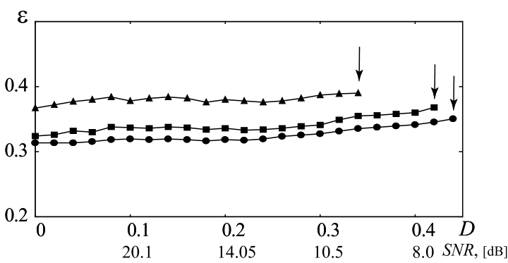
Figure 1: Dependence of the threshold of the GS regime onset in two unidirectionally coupled logistic maps (13) on the intensity of noise (the SNR values corresponding to the noise intensities are also shown) for different values of the control parameters: $\lambda_{x}=3.75$, $\lambda_{y}=3.75$ ($\bullet$), $\lambda_{x}=3.75$, $\lambda_{y}=3.79$ ($\blacksquare$), $\lambda_{x}=3.75$, $\lambda_{y}=3.9$ ($\blacktriangle$). Critical values of the noise intensity $D_{c}$, up to which the GS regime in system (13) is observed, are marked by arrows

On the horizontal axis the signal to noise ratios (SNR, [dB]) corresponding to these noise intensities are also indicated . One can easily see that the threshold value of the coupling parameter $\varepsilon$ is almost independent on the intensity of noise $D\in[0;D_{c}]$ where $D_{c}$ shown in Fig. 1 by arrows, depends on the control parameter values, $D_{c}=D_{c}(\lambda_{x},\lambda_{y})$. For the selected values of the control parameters $D_{c}\in[0.38;0.44]$ ($\rm SNR\in[8.5;7.2]dB$, respectively), i.e. the GS regime in unidirectionally coupled logistic maps (13) is stable to noise up to the power of noise comparable with the chaotic signal one.

To explain the reasons of stability of the GS regime with respect to external noise we use the modified system approach described in Section 1. At the same time, due to the fact that the theory of the stability of the GS regime to noise proposed in Section 1, is applicable to flow systems, and the noise added in system (13) is multiplicative, there are several peculiarities to be discussed bellow. Therefore, we use the modified system approach with regard to the system with discrete time and consider the modified logistic map:

$$z_{n+1}=f_{m}(z_{n},\lambda_{y})=(1-\varepsilon)f(z_{n},\lambda_{y}).$$ (14)

One can see that the modified system (14) may be rewritten in the form

$$z_{n+1}=az_{n}(1-z_{n}),$$ (15)

where $a=\lambda_{y}(1-\varepsilon)$. It is clearly seen that the term $-\varepsilon f(z_{n},\lambda_{y})$ brings additional dissipation in system (14). The local phase volume contraction is characterized by means of the modulus of the derivative

$$\left|\displaystyle\frac{dz_{n+1}}{dz_{n}}\right|=(1-\varepsilon)\left|f^{\prime}_{z_{n}}(z_{n},\lambda_{y})\right|$$ (16)

where the modulus of multiplier ${|\displaystyle f^{\prime}_{z_{n}}(z_{n},\lambda_{y})|}=\lambda_{y}|1-2z_{n}|$ characterizes the phase volume contraction in the autonomous response system. The case of ${\left|dz_{n+1}/dz_{n}\right|=1}$ corresponds to the non-dissipative dynamics whereas $\left|{dz_{n+1}}/{dz_{n}}\right|=0$ relates to the infinitely large dissipation. One can see that, as in the case of flow systems, the dissipation in the modified system is greater than in the response one and it increases with the growth of the coupling strength $\varepsilon$, ($0<\varepsilon<1$). Bifurcation diagram characterizing its behavior with the increase of $\varepsilon$-parameter is shown in Fig. 2,a.

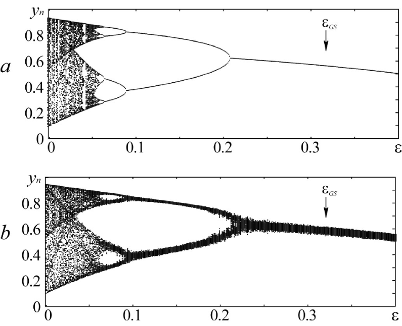
Figure 2: Bifurcation diagrams of the modified logistic map (15) in the absence (a) and presence (b) of noise (the noise is introduced in system (15) in the same way as in Eq. (13)). The control parameter $\lambda_{y}=3.79$ in both cases, the noise intensity $D=0.1$ in (b). The coupling parameter values $\varepsilon_{GS}=0.32$ corresponding to the GS regime (obtained by means of conditional Lyapunov exponent computation) are marked by arrow in both cases

The value of parameter $\varepsilon$ corresponding to the onset of the GS regime (obtained by means of conditional Lyapunov exponent computation, see Sec. 1) is marked by arrow. One can see that for a coupling parameter strengths corresponding to the onset of the GS regime in system (13), in full agreement with the arguments discussed in Aeh:2005_GS:ModifiedSystem , the modified system (15) demonstrates the periodic oscillations. External noise does not almost change the characteristics of the modified system and, therefore, it does not affect the threshold of the GS regime arising. Bifurcation diagram of the modified logistic map in the presence of noise of intensity $D=0.1$ is shown in Fig. 2,b. The noise is introduced in system (15) in the same way as in Eq. (13), i.e.

$$z_{n+1}=f_{m}(z_{n},\lambda_{y})+\varepsilon Df(\xi_{n},\lambda_{x})$$ (17)

to provide the same noise influence as in the coupled logistic maps. The level of noise is quite sufficient in comparison with the signal amplitude what is clearly seen from the kind of bifurcation diagram. At the same time, it is easy to see that noise does not shift the bifurcation points in this case but only leads to a noisiness of the system regime. Therefore, in the considered case one can say that, despite of the large amplitude, the external noise does not affect the threshold of the GS regime onset. The further increase of the noise intensity $D>D_{c}$ results in the runaway of the representation point to infinity.

The reasons of the jump of the representation point to infinity can be explained in the following way. Logistic map in autonomous regime

$$x_{n+1}=f(x_{n},\lambda),$$ (18)

is known to have a finite basin of attraction, i.e., depending on the choice of the initial conditions, for the values of the control parameter $\lambda$ mentioned above it demonstrates either chaotic regime or the jump of representation point to infinity Schuster:1984_CHAOS_BOOK . To provide the chaotic regime in system (18) we have to specify initial condition in range $x_{0}\in[0;1]$, with the representation point remaining in this range during the evolution of the system for an infinitely long time, at that the maximal value of $f(x_{n})=f_{max}=\lambda/4$ would be achieved if $x_{n}=1/2$. At the same time, it is clear that external noise could make it go out the range mentioned above.

The similar effect takes place for systems (13). One can estimate the intensity of noise $D_{c}$ corresponding to the jump of representation point of the response system to infinity. For this purpose we consider the behavior of the drive and response systems of Eq. (13). First equation corresponds to the drive system and is not affected by the influence of external noisy or chaotic signal. Therefore the most probable value of $f(x_{n})=\langle f_{x}\rangle$ where $\langle f_{x}\rangle$ is a statistical mean of $f(x_{n})$ (due to the properties of the autonomous logistic map). The maximal values of $f(y_{n})$ and $f(\xi_{n})$ would be equal to $f_{max}$ because of the uniform character of the probability distribution of the random value $\xi_{n}$ and the arguments discussed above. Due to the fact that a random variable $\xi_{n}$ could not be negative the jump of the representation point from the range $[0;1]$ could be performed only through a right boundary of such range. Therefore the maximal value of $y_{n+1}$ is $1$. Substituting all quantities into the second equation of (13) and assuming $\varepsilon=\varepsilon_{c}$ ($\varepsilon_{c}$ corresponds to the threshold value of the GS regime onset without noise) we can estimate the approximate values of the noise intensity $D_{c}$ up to which the jump of representation point to infinity does not take place. Our calculations show that

$$D_{c}\approx\frac{4-4\varepsilon_{c}\langle f_{x}\rangle-(1-\varepsilon_{c})\lambda_{y}}{\varepsilon_{c}\lambda_{x}},$$ (19)

i.e. ${D_{c}\approx 0.5}$ for the control parameter values ${\lambda_{x}=\lambda_{y}=3.75}$, ${D_{c}\approx 0.48}$ for ${\lambda_{x}=3.75}$, ${\lambda_{y}=3.79}$ and ${D_{c}\approx 0.42}$ for ${\lambda_{x}=3.75}$, ${\lambda_{y}=3.9}$, that agrees well with the results of direct numerical calculations. Therefore, the GS regime for logistic maps, having a limited basin of attraction, exhibit the stability with respect to noise in the large, but limited range of the noise intensity.

In the considered case the GS regime destruction is connected with the jump of representation point to infinity, which could be considered as an attraction of it to the second coexisting attractor being at the infinity Grebogi:1983_Basins . Note, if the coexisting attractor was characterized by the limited basin of attraction, depending on the type of the regime being realized in the response system (and, correspondingly, to the second attractor), the increase or decrease of the threshold value of the GS regime would be observed with the growth of the noise intensity Guan:NoiseGS:2006 .

The another important question is the stability of GS with respect to the external noise in the case when statistically independent noise sources affect the drive and response systems

$$\begin{array}[]{l}x_{n+1}=f(x_{n},\lambda_{x})+\varepsilon Df(\zeta_{n},\lambda_{x}),\\ y_{n+1}=f(y_{n},\lambda_{y})+\varepsilon(f(x_{n},\lambda_{x})+Df(\xi_{n},\lambda_{x})-f(y_{n},\lambda_{y})),\end{array}$$ (20)

where $\zeta_{n}$ is a stochastic process with the probability density distributed uniformly in $[0;1]$-range. Applying the arguments similar to the last one described for the system (13) to system (20), we can estimate the intensity of noise $D_{c}^{d}$ corresponding to the jump of the representation point of the drive system to infinity. It is clear that due to the absence of the dissipative term in the drive system the jump of representation point in it would take place for a less values of the noise intensity than for the response one. In this case the GS regime is stable to the noise influence until ${D<D_{c}^{d}}$, where

$$D_{c}^{d}\approx\frac{1-\lambda_{x}/4}{\varepsilon_{c}\lambda_{x}/4}\approx 0.2.$$ (21)

The further increase of the noise intensity $D>D_{c}^{d}$ results in the chaotic regime destruction in the drive system. Therefore, the values $D>D_{c}^{d}$ are unapplicable for (20), since the jump of the representation point towards infinity in the drive system is observed.

Numerical calculations confirm the results obtained analytically. In Fig. 3 dependencies of the critical values of the coupling parameter strength corresponding to the GS regime arising for different values of the control parameters are shown (the SNR values are also indicated in the second horizontal axis).

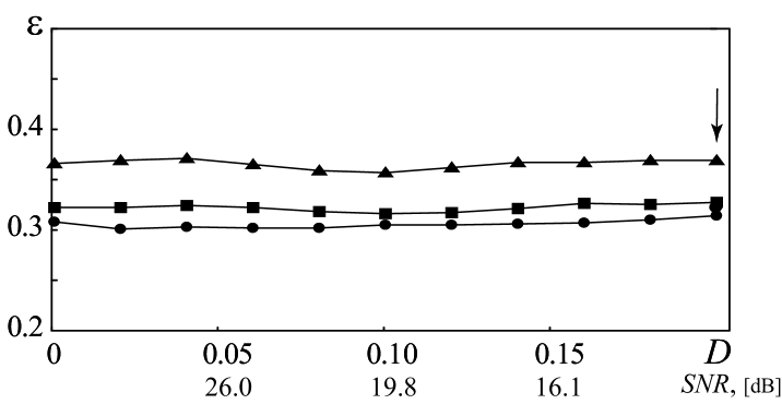
Figure 3: Dependence of the threshold of the GS regime onset in two unidirectionally coupled logistic maps (20) in the presence of noise both in the drive and response on its intensity (the SNR values corresponding to the noise intensities are also shown) for different values of the control parameters: $\lambda_{x}=3.75$, $\lambda_{y}=3.75$ ($\bullet$), $\lambda_{x}=3.75$, $\lambda_{y}=3.79$ ($\blacksquare$), $\lambda_{x}=3.75$, $\lambda_{y}=3.9$ ($\blacktriangle$)

As in the case of the absence of noise in the drive system external noise does not affect the threshold value of the GS regime onset. The very similar result is obtained in the case when both the drive and response systems are under the influence of the common noise source, i.e., $\xi_{n}\equiv\zeta_{n}$.

It should be noted that the GS regime is also robust in the limited range against the perturbations in the control parameters by noise. Therefore, one can conclude that for unidirectionally dissipatively coupled systems with discrete time the GS regime would exhibit the stability with respect to noise.

2.2 Rössler systems

As a second example we consider two unidirectionally coupled flow Rössler oscillators:

$$\begin{array}[]{ll}\dot{x}_{1}=-\omega_{x}x_{2}-x_{3}+D_{1}\zeta,\\ \dot{x}_{2}=\omega_{x}x_{1}+ax_{2},\\ \dot{x}_{3}=p+x_{3}(x_{1}-c),\\ \\ \dot{u}_{1}=-\omega_{u}u_{2}-u_{3}+\varepsilon(x_{1}+D_{2}\xi-u_{1}),\\ \dot{u}_{2}=\omega_{u}u_{1}+au_{2},\\ \dot{u}_{3}=p+u_{3}(u_{1}-c),\end{array}$$ (22)

where $\mathbf{x}(t)=(x_{1},x_{2},x_{3})^{T}$ and $\mathbf{u}(t)=(u_{1},u_{2},u_{3})^{T}$ are the vector-states of the drive and response systems, respectively, $a=0.15$, $p=0.2$, $c=10$, $\omega_{x}$ and $\omega_{u}=0.95$ are the control parameter values, $\varepsilon$ is a coupling parameter. The parameters $\omega_{x,u}$ define the natural frequencies of the drive and response system oscillations. The terms $D_{1}\zeta$, $D_{2}\xi$ simulate the external noise influenced on the drive and response systems. Here $\xi$ and $\zeta$ are statistically independent stochastic Gaussian processes described by the following probability distribution

$$p(\xi)=\frac{1}{\sqrt{2\pi}\sigma}\exp\left(-\frac{(\xi-\xi_{0})^{2}}{2\sigma^{2}}\right),$$ (23)

where $\xi_{0}=0$ and $\sigma=1.0$ are the mean value and variance. Parameters $D_{1,2}$ define the intensities of the noise added in the drive and response systems, respectively.

To integrate the stochastic equations (22) we have used the four order Runge-Kutta method adapted for the stochastic differential equations Nikitin:1975_StochDE_eng with time discretization step $\Delta t=0.001$. The modified Runge-Kutta method is applicable for delta-correlated Gaussian white noise used frequently in our Manuscript. At the same time, for the integration of the stochastic differential equations in the case of the other types of noise we have used one-step Euler method. For the GS regime detection the auxiliary system method described in Section 1 has been used.

At first, we consider the behavior of chaotic systems (22) in the presence of noise influenced only on the response system, i.e. $D_{1}=0$, $D_{2}=D$.

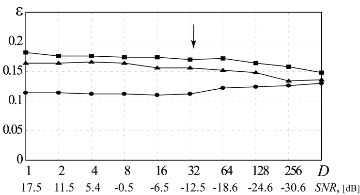
Figure 4: Dependence of the boundary value corresponding to the GS regime arising in two unidirectionally coupled Rössler systems with additive stochastic term (22) on the noise intensity $D$ (the SNR values corresponding to the noise intensities are also shown) for different values of the drive system parameter $\omega_{x}$: $\omega_{x}=0.99$ ($\bullet$), $\omega_{x}=0.95$ ($\blacksquare$), $\omega_{x}=0.91$ ($\blacktriangle$). The critical value of the noise intensity $D_{c}$ up to which the boundary value of the GS regime does not almost depend on the noise intensity is marked by arrow

Fig. 4 shows the dependence of the threshold of the GS regime onset on the noise amplitude $D$ (the SNR value) for three different values of the control parameter $\omega_{x}$ and fixed values of the other control parameters. To possess all necessary knowledge about influence of noise on the system under study we have chosen values of the parameter $\omega_{x}$ in the different ranges of the parameter mismatch where the different mechanisms of the synchronous regime arising have been shown to take place Harmov:2005_GSOnset_EPL . Parameter $\omega_{x}=0.99$ corresponds to the case of the relatively large values of the frequency detuning whereas $\omega_{x}=0.95$ (interacting systems are identical) and $\omega_{x}=0.91$ relate to the small ones. It is easy to see that independently on the value of the control parameter $\omega_{x}$ the threshold of the GS regime onset does not almost depend on the noise amplitude $D\in[0;40]$ (${\rm SNR>-14.5dB}$). Even for a great values of the noise intensity GS arises practically for the same values of the coupling parameter strength $\varepsilon$ as for a noiseless case. Typical signals $s(t)=x_{1}(t)+D\xi(t)$ affecting the response and auxiliary systems both in the absence and presence of noise as well as the phase portraits of the response system and $(u_{1},v_{1})$-planes characterizing the response and auxiliary system behavior before (b,c,g,h) and after (d,e,i,j) the GS regime onset are shown in Fig. 5.

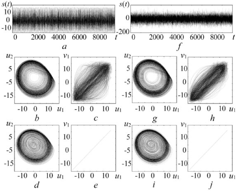
Figure 5: Signals $s(t)$ affecting the response and auxiliary systems (a,f), phase portraits (b,d,g,i) and $(u_{1},v_{1})$-planes characterizing the response and auxiliary system behavior (c,e,h,j) before ($\varepsilon=0.05$) and after ($\varepsilon=0.114$) the GS regime onset in unidirectionally coupled Rössler systems with $\omega_{d}=0.99$, respectively. Pictures (a–e) correspond to the noiseless case ($D=0$) whereas (f–j) refer to the noise one ($D=40$)

Pictures (a–e) correspond to the noiseless case whereas (f–j) refer to the presence of noise of great intensity $D=40$ affecting the response system (in the last case the signal is similar to the stochastic one, with its amplitude being in approximately 10 times more in comparison with the noiseless case, compare Fig. 5,a,f). One can easily see that characteristics of the response systems are changed slightly with the noise intensity increasing (compare pictures b,d and g,i, respectively) and the boundary value of the GS regime remains practically the same. The causes determining the stability of the GS regime with respect to the external noise influence are the same as in the already considered case of the logistic maps (13) and could also be explained by the modified system approach. One can say that for unidirectionally coupled Rössler systems the noise of great intensity does not change the characteristics of the modified system

$$\begin{array}[]{l}\dot{z}_{1}=-\omega_{u}z_{2}-z_{3}-\varepsilon z_{1},\\ \dot{z}_{2}=\omega_{u}z_{1}+az_{2},\\ \dot{z}_{3}=p+z_{3}(z_{1}-c),\end{array}$$ (24)

where $\mathbf{z}=(z_{1},z_{2},z_{3})^{T}$ is the vector state of the modified system and, as a consequence, of the response one. By the analogy with the logistic maps the bifurcation diagrams for the modified Rössler system are shown in Fig. 6.

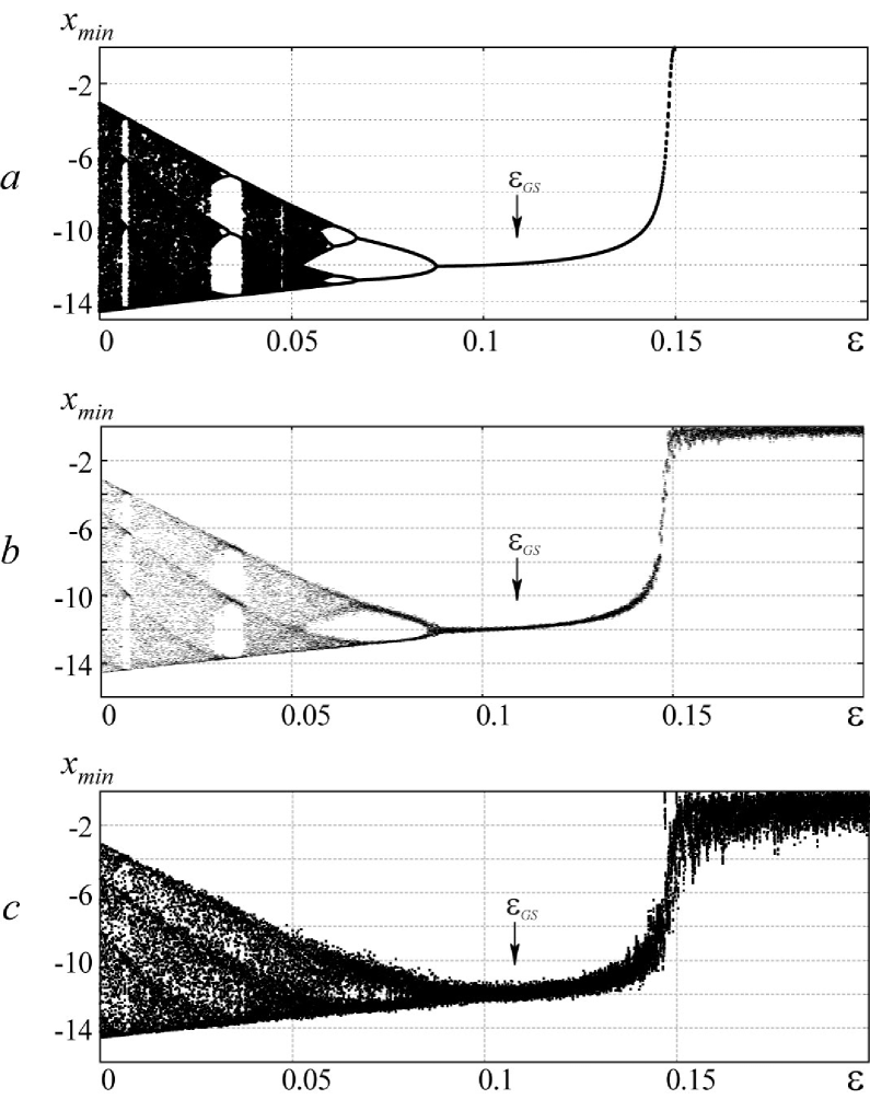
Figure 6: Bifurcation diagrams of the modified Rössler system (24) in the absence (a) and presence (b,c) of noise (the noise is introduced in system (24) in the same way as in Eq. (22)). The control parameter $\omega_{x}=0.99$ in all considered cases, the noise intensity $D=10$ in (b) and $D=40$ in (c). The coupling parameter values $\varepsilon_{GS}=0.112$ corresponding to the GS regime (obtained by means of auxiliary system method, see Sec. 1) are marked by arrow in all cases

Fig. 6,a corresponds to the noiseless case ($D=0$) whereas in Fig. 6,b,c the modified Rössler systems with additive noise of the different intensities ($D=10$ and $D=40$, respectively) (the noise is introduced in system (24) in the same way as in Eq. (22)) are shown. Independently on the noise intensity for the selected values of the control parameters the cycle-1 periodic oscillations are observed in the modified system (24) (see also Aeh:2005_GS:ModifiedSystem ).

The external noise does not shift the bifurcation points and, therefore, does not affect the boundary value of the GS regime. Therefore, we can conclude that the mechanisms determining the GS regime stability are the same as for the system with discrete time (13). At the same time, since the basin of attraction in the Rössler system is unbounded, the effect of the GS regime destruction described above in Section 2.1 could not be observed.

One more interesting question to be discussed is the relationship between the onset of the GS and CS regimes. According to the consideration made on the base of the modified system approach, GS and CS have the same mechanisms. At the same time, as we have mentioned in Section 1, the stability of the GS regime is stronger than the CS one. To confirm this statement we have analyzed the CS regime arising in unidirectionally coupled identical Rössler systems (22) with $\omega_{d}=\omega_{r}=0.95$ and compared obtained results with the last one for the GS. Our calculations show that in the absence of noise CS arises in this case for $\varepsilon=0.19$, whereas GS takes place for $\varepsilon\geq 0.184$. Adding noise of small intensity $D=0.1$ results in the appearance of on-off intermittency Ott:1994_BlowoutBifurcation between the drive and response systems, at that the threshold value of the CS regime grows up, but the GS regime is still observed (see Fig 4 and Fig. 7).

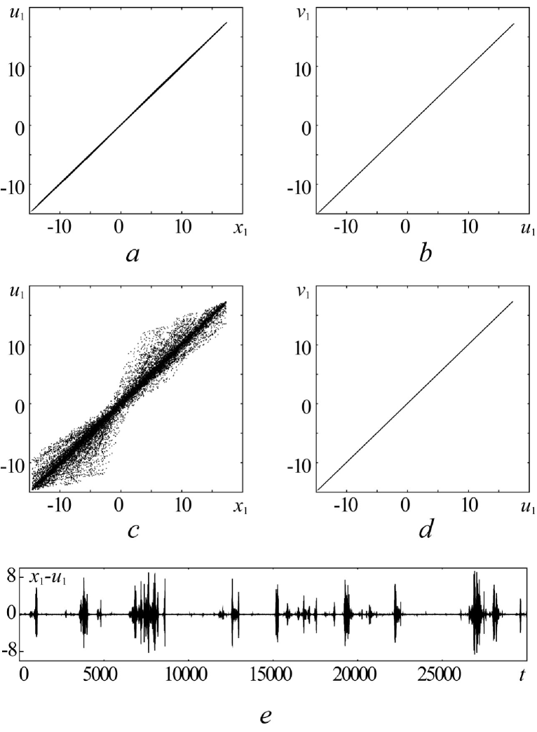
Figure 7: $(x_{1};u_{1})$- and $(u_{1};v_{1})$-planes characterizing the drive and response (a,c) and response and auxiliary (b,d) Rössler system behavior in the case of the absence (a,b) and the presence (c,d) of noise in the response system (the noise intensity ${D=0.1}$, the coupling strength ${\varepsilon=0.19}$). The difference between the drive and response system states in the presence of noise (${D=0.1}$, ${\varepsilon=0.19}$) shown in Fig. 7, e illustrates the presence of on-off intermittency. Parameter of the drive system ${\omega_{d}=0.95}$

For the very large values of the noise intensity when the power of noise is much more than the Rössler system signal one ($D\gtrsim 400$, $\rm SNR\lesssim-34.5$) the detected synchronous regime may be treated as the noise-induced synchronization, being the manifestation of the GS regime in the case when stochastic signal instead of the deterministic one is affected the response and auxiliary systems Hramov:2006_PLA_NIS_GS . In other words, the deterministic signal from the drive system practically does not play role and may be neglected in comparison with the stochastic one. At that, the boundary value of the synchronous regime onset should not depend on the control parameter of the drive system $\omega_{x}$ (see, Fig. 4 for a large $D$) and is determined mainly by the characteristics of the noise signal. Therefore, for the noise intensities $D\gtrsim D_{c}=45$ ($\rm SNR<-15.5dB$) (shown in Fig. 4 by arrow) the threshold value of the synchronous regime may start increasing or decreasing depending on the value of the control parameter detuning.

It should be noted that the weak dependence of the threshold value of the GS regime onset in the wide range of the noise intensity $D$ takes place if the amplitude $D_{1}$ of the additive noise term in equations (22) is not equal to zero. We have chosen it to be equal to $D_{1}=\varepsilon D$. These dependencies for a different values of the drive system parameter $\omega_{x}$ are shown in Fig. 8. Such behavior of interacting systems in the presence of noise is fully defined by mechanisms described above in this subsection.

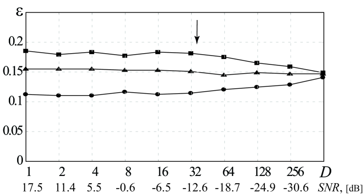
Figure 8: Dependence of the boundary value of the GS regime arising in two unidirectionally coupled Rössler systems in the case when statistically independent noise sources of intensity $D$ affect the drive and response on the noise intensity $D$ (the SNR values corresponding to the noise intensities are also shown) for different values of the drive system parameter $\omega_{x}$: $\omega_{x}=0.99$ ($\bullet$), $\omega_{x}=0.95$ ($\blacksquare$), $\omega_{x}=0.91$ ($\blacktriangle$). The critical value of the noise intensity $D_{c}$ up to which the boundary value of the GS regime does not almost depend on the noise intensity is marked by arrow

Therefore, one can say that in both considered cases (maps and flows) in the wide range of the noise intensity the external noise does not practically affect the threshold of the GS regime arising. Hence, we can say about stability of the GS regime with respect to external noise in dynamical systems with a few number of degrees of freedom.

2.3 Ginzburg-Landau equations

As a third example we consider the GS regime arising in spatially extended self-oscillating media described by the complex Ginzburg-Landau equations (CGLE). The system under study is represented by a pair of unidirectionally dissipatively coupled complex Ginzburg-Landau equations (CGLE’s) being under influence of distributed in space source of the white noise. Equations describing such system may be written as

$$\begin{array}[]{l}\displaystyle\frac{\partial u}{\partial t}=u-(1-i\alpha_{d})|u|^{2}u+(1+i\beta_{d})\frac{\partial^{2}u}{\partial x^{2}}+\\ \qquad+\varepsilon\tilde{D}\xi(x,t),\quad x\in[0,L],\end{array}$$ (25)

$$\begin{array}[]{l}\displaystyle\frac{\partial v}{\partial t}=v-(1-i\alpha_{r})|v|^{2}v+(1+i\beta_{r})\frac{\partial^{2}v}{\partial x^{2}}+\\ \qquad+\varepsilon(\tilde{D}\zeta(x,t)+u-v),\quad x\in[0,L].\end{array}$$ (26)

Equation (25) describes the drive system and equation (26) corresponds to the response one. It is known that in two unidirectional CGLE’s the GS regime may take place Hramov:2005_GLEsPRE . In our investigation the parameters of the drive system are chosen as $\alpha_{d}=1.5$, $\beta_{d}=1.5$. To study the generalized synchronization of the nonidentical systems we have chosen the different values of control parameters $\alpha_{r}\in[3;5]$ and $\beta_{r}\in[3;5]$ for the response system (26). The choice of such values of the control parameters results in the autonomous systems being in the spatiotemporal chaotic regime. Parameter $\varepsilon$ determines the strength of the unidirectionally dissipative coupling between the response and drive systems, with the interaction of them being in each point of space. The terms $\tilde{D}\xi(x,t),\zeta(x,t)$ simulate complex model noise with Gaussian distribution of the random values $\xi(x,t),\zeta(x,t)$ with zero mean value:

$$\begin{array}[]{ll}\langle\zeta(x,t)\rangle=0,\\ \langle\zeta(x,t)\zeta(x^{\prime},t^{\prime})\rangle=\delta(x-x^{\prime})\delta(t-t^{\prime}),\end{array}$$ (27)

$\tilde{D}$ defines the noise intensity.

Equations (25)–(26) have been solved with periodic boundary conditions ${u(x,t)=u(x+L,t)}$ and ${v(x,t)=v(x+L,t)}$, with all numerical calculations being performed for a fixed system length $L=40\pi$ and random initial conditions. To evaluate (25)–(26) the standard numerical scheme for integration of the stochastic partial differential equations Garcia-Ojalvo:1999_NoiseBook has been used, the value of the grid spacing is $\Delta x=L/1024$, the time step of the scheme is $\Delta t=0.0002$.

To detect the presence of the GS regime we have used the auxiliary system method described in Section 1. At that, we have assumed that auxiliary system $v_{a}(t)$, also satisfying (26), has been under influence of the noise source of the intensity $\tilde{D}$ equal to the last one for the response system. As an criterion of the GS regime arising we have chosen the following one. The GS regime takes place when the mean standard deviation of the response $v$ and auxiliary $v_{a}$ system states satisfies the following condition:

$$\frac{1}{T}\int_{T}\int_{0}^{L}|v(x,t)-v_{a}(x,t)|^{2}<\delta,$$ (28)

where $\delta=10^{-5}$.

Fig. 9 shows the dependence of the boundary value of the GS regime onset $\varepsilon$ on the noise intensity $\tilde{D}$ (SNR value) for several values of the control parameters of the response system.

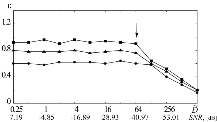
Figure 9: Dependence of the boundary value of the GS regime onset in the coupled CGLE’s on the noise intensity $\tilde{D}$ (the SNR values corresponding to the noise intensities are also shown) for different values of the control parameters of the response system: $\alpha_{r}=3,\beta_{r}=3$ ($\bullet$), $\alpha_{r}=4,\beta_{r}=4$ ($\blacktriangle$), $\alpha_{r}=5,\beta_{r}=5$ ($\blacksquare$). The critical value of the noise intensity $D_{c}$ up to which the boundary value of the GS regime does not almost depend on the noise intensity is marked by arrow

One can easily see that the noise of intensity ${\tilde{D}\in[0;64]}$ ($\rm SNR\geq-41dB$) does not almost affect the threshold of the GS regime onset in spatially extended systems described by the Ginzburg-Landau equations. The time-space diagrams characterizing the behavior of unidirectionally coupled spatially extended media before and after the GS regime onset both in the absence and presence of noise are shown in Fig. 10.

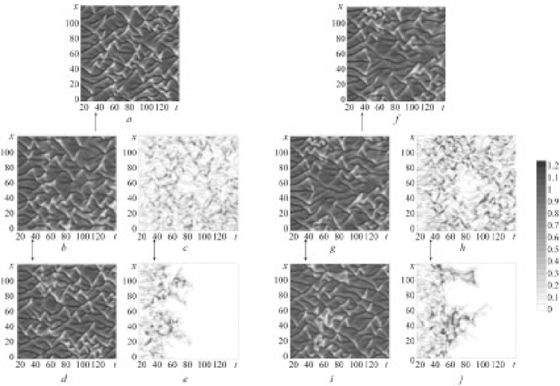
Figure 10: The spatio-temporal diagrams characterizing behavior of the drive (a,f) and response (b,d,g,i) systems (25)–(26) as well as the dependencies of the module of the difference between the states of the response and auxiliary systems $|v-v_{a}|$ (c,e,h,j) for cases of absence (c,h) ($\varepsilon=0.2$) and presence (e,j) ($\varepsilon=0.8$) of the GS on time $t$ and space $x$. The control parameter values for the response system have been selected as $\alpha_{r}=\beta_{r}=3$. The time moments marked by arrows correspond to the coupling switching-on between the drive and response systems. Pictures (a–e) correspond to the noiseless case ($\tilde{D}=0$) whereas (f–j) refer to the noise one ($\tilde{D}=0.4$)

Pictures (a–e) correspond to the case of the absence of noise both in the drive and response systems whereas in the pictures (f–j) the white noise of intensity $\tilde{D}=0.4$ affects both the drive and response. Pictures (a,f) characterize the drive system behavior, whereas the other ones refer to the response system one before (b,g) and after (d,i) the GS regime onset. Fig. 10,c,e,h,j shows the spatiotemporal distributions of the module of the difference between the states of the response and auxiliary systems $|v-v_{a}|$ for cases of the absence (c,h) and the presence (e,j) of the GS regime. One can easily see, that in the second cases (e,j) the difference of the states of the response and auxiliary systems in every point of space tends to be zero after coupling begins, which means the presence of the GS between the drive and response CGLE’s. It should be noted that the length of the transient process preceded to the GS regime onset is occurred to be rather more in the case of the presence of noise whereas the threshold value of the GS regime onset is the same as in the noiseless case. Moreover, one can easily see that spatio-temporal diagrams characterizing the response system behavior are similar to each other both in the presence and absence of noise (compare pictures (b,d) with (g,i), respectively).

The stability of the GS regime in Ginzburg-Landau equations with respect to noise is determined by the same mechanisms, as in the cases of the systems with a few number of degrees of freedom considered in the previous subsections 2.1 and 2.2. As well as for the logistic maps and Rössler systems, the modified system approach may be used for the explanation of the observed phenomenon. Indeed, the noise of a large enough intensity does not almost affect the characteristics of the modified Ginzburg-Landau equation

$$\begin{array}[]{l}\displaystyle\frac{\partial v_{m}}{\partial t}=v_{m}-(1-i\alpha_{r})|v_{m}|^{2}v_{m}+\\ \displaystyle\quad+(1+i\beta_{r})\frac{\partial^{2}v_{m}}{\partial x^{2}}-\varepsilon v_{m},\quad x\in[0,L]\end{array}$$ (29)

(and, as a consequence, of the response one), as well as in the case of Ginzburg-Landau equation with the added constant term Hramov:2008_INIS_PRE . Therefore, the noise does not change the threshold value of the GS regime onset. At the same time, as it has been discussed in Section 1, the boundary value of the coupling parameter $\varepsilon$ may start changing if the noise intensity is a very great (${\tilde{D}>64}$, ${\rm SNR<-41dB}$). It is easy to see from Fig. 9 that for such values of the noise intensity the boundary value of the GS regime starts decreasing. For the very large intensities $D$ the coupling value $\varepsilon_{GS}$ corresponding to the boundary of the GS regime tends to the constant value which does not depend on the the control parameters $\alpha$ and $\beta$ of the spatially extended media. Such behavior of the boundary value of the GS regime onset, as in the case of unidirectionally coupled Rössler systems considered in Section 2.2, is connected with the noise-induced synchronization regime realization.

Nevertheless, the noise of a large enough intensity does not almost alter the threshold value of the coupling parameter strength between two unidirectionally coupled Ginzburg-Landau equations. In this case one can say about stability of the GS regime with respect to noise in the coupled spatially extended self-oscillating media.

So, having considered three different examples of model systems (discrete maps, flow systems, spatially-extended media) we can come to the conclusion that the GS regime demonstrates the significant stability with respect to noise in a wide range of the values of the external noise intensity.

3 Experimental study of the GS onset in chaotic circuits in the presence of noise

To confirm the theoretical and numerical results given in the previous sections we have also studied experimentally the dynamics of the chaotic oscillator driven by the external chaotic signal in the presence of noise. In the experiment we have used the simple electronic circuit where all parameters including noise amplitude may be controlled precisely.

The experimental setup is shown in Fig. 11. As a basic element of the scheme we have used an electronic circuit with nonlinear converter and linear feedback loop similar to the one described in Rulkov:1996_SynchroCircuits ; Hramov:2007_TypeIAndNoise (it is shown in Fig. 11 by dashed rectangle). Since the generator is capable to demonstrate both periodic and chaotic oscillations depending on the choice of the parameter $\alpha$ of nonlinear converter, it has been selected in such a way for the generated signal to be chaotic (quantitative values of all control parameters of the circuit are presented in the captions of Fig. 11 and 12). Chaotic generator has been connected to DAC/ADC board L-Card L-783 installed into personal computer (PC) whereby we have recorded the dynamics of potential on the capacitors $C$ and $C^{\prime}$. As a drive signal we have used the last one generated by the circuit described above, digitized by ADC with further reconstruction by DAC. The drive signal has been introduced into the circuit via dissipative unidirectional coupling of variable dissipation value (see Fig. 11). The noise signal has been produced with Agilent 33220 function generator, digitized and additively introduced into the coupling device (as it has been shown in Fig. 11). Characteristics of the noise are close to the Gaussian one. Oscillations of the response system have been also digitized with ADC board and transferred to personal computer for further numerical processing.

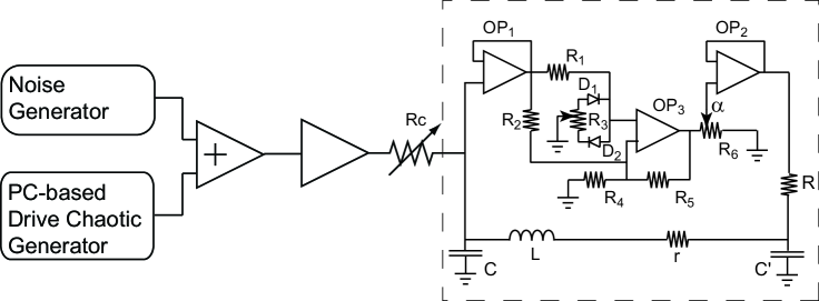
Figure 11: Block diagram of experimental setup. Chaotic generator layout is shown by dashed rectangle. Here $C$=330 nF, $C^{\prime}$=150 nF, $R$=630 $\Omega$, $r$=56 $\Omega$, $L$=3.3 mH, $OP_{1,2}$ – TL082, $OP_{3}$ – LF356N, $D_{1,2}$ – 1N4148, $R_{1}$=2.7 $k\Omega$, $R_{2}$=$R_{4}$=7.4 $k\Omega$, $R_{3}$=100 $\Omega$, $R_{5}$=186 $k\Omega$, $R_{6}$=4.7 $k\Omega$, $RC^{\prime}$, $rLC$ – low-pass filters, $\alpha$ is parameter of nonlinear converter, $R_{c}$ is a coupling resistance

As we have mentioned above, one of the easiest ways to detect the presence of the GS regime is the use of an auxiliary system, i.e. an additional response circuit, which is a replica of the main one. But creation of the auxiliary system with parameters completely equal to the response system ones is one of the most conceptual problems in the experimental study of the GS regime. To solve this problem we have used an approach analogous to the one discussed in Uchida:2003_GSLaserPRL . As it has been specified above, the signal from the drive system with additive noise has been preliminary recorded on PC. Therefore, it is evident that in this case the response system could be subjected to the influence of identical drive signal (with additive noise) any number of times. For the realization of an auxiliary system method it is quite sufficient to affect the response system by the drive signal twice, alternating the period of the influence with the time interval of autonomous dynamics (to provide the different initial conditions), and then compare obtained data numerically.

The experiment has been performed for three main cases: (i) chaotic attractors both in the drive and response systems have identical band structure; (ii) chaotic regime with band attractor has influenced on the regime with double scroll attractor; (iii) chaotic attractors both in the drive and response systems have a double scroll structure. Typical phase portraits of considered regimes are shown in Fig.12 (band attractor (a) and double scroll attractor (b)). The corresponding values of the control parameter $\alpha$ are indicated in the caption.

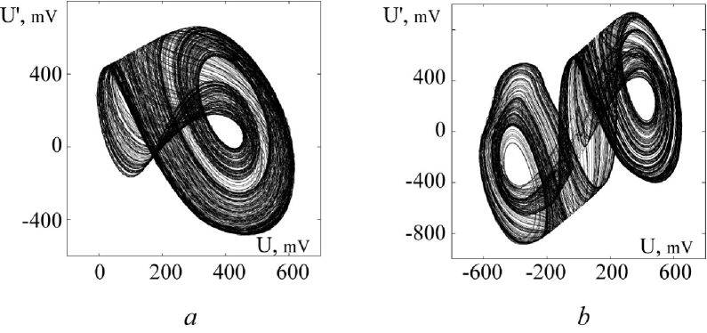
Figure 12: Typical phase portraits of chaotic regimes observed in experiment: (a) band attractor ($\alpha\sim 0.15$), (b) double scroll attractor ($\alpha\sim 0.25$)

Each case has been studied in the presence of Gaussian noise of different intensity. For experimental data the noise intensity has been calculated as a ratio ${D=P_{N}/P_{CS}}$ of a power of the noise signal $P_{N}$ to the power of chaotic signal $P_{CS}$.

Figure 13 shows the dependence of the coupling strength value $\displaystyle\varepsilon=\frac{1}{R_{c}}\sqrt{\frac{L}{C}}$ corresponding to GS regime onset on the noise intensity for three cases mentioned above.

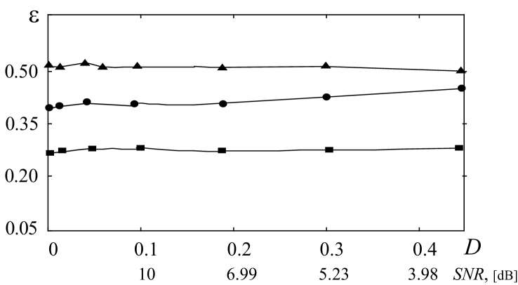
Figure 13: Coupling strength value corresponding to the GS regime onset as a function of noise intensity (the SNR values corresponding to the noise intensities are also shown) in the cases when chaotic attractors both in drive and response systems have the band structure ($\blacksquare$); drive system in the band chaotic regime influences on the response system in chaotic regime with the double scroll attractor ($\bullet$); chaotic attractors both in drive and response systems have a double scroll structure ($\blacktriangle$)

One can see that in the range of noise intensity [0; 0.5] the threshold value remains nearly constant. Typical signals from the drive system with and without additive noise affecting the response one as well as the phase portraits of the response system and $(U,V)$-planes characterizing the response and auxiliary system behavior both in the absence and presence of the GS regime in chaotic circuits in the case (i) are shown in Fig. 14.

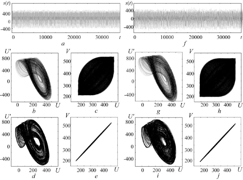
Figure 14: Signals from the drive chaotic circuit without (a) and with (f) additive noise affecting the response circuit, phase portraits of the response system (b,d,g,i) and $(U,V)$-planes characterizing the response and auxiliary system behavior (c,e,h,j) before ($\varepsilon=0.22$) and after ($\varepsilon=0.34$) the GS regime onset. The control parameters of the chaotic circuit has been chosen in such a way that both the drive and response systems in autonomous regime are characterized by the band attractors. Pictures (a–e) correspond to the noiseless case ($D=0$) whereas (f–j) refer to the noise one ($D=0.4$)

One can easily see that characteristics of the response circuit have not been changed noticeably with the appearance of noise. Analogous situation takes place in unidirectionally coupled chaotic circuits with initially double-scroll chaotic attractors in the one and both of them. One can say that in all considered cases the modified system (i.e. considered generator with additional dissipation) demonstrates the cycle-1 periodic oscillations. Further increase of the noise intensity (when it becomes greater than the intensity of the deterministic signal) may result in the monotonous growth of the GS boundary value.

So, the experimental results satisfy the stability of the GS regime with respect to noise. They are also in a good agreement with the data obtained theoretically and numerically.

Conclusions

In conclusion, we have analyzed both theoretically and experimentally the influence of noise on the GS regime in different unidirectionally dissipatively coupled identical chaotic systems with mismatched parameters with a small number of degrees of freedom as well as spatially extended media. The dependencies of the GS regime boundary on the noise intensity in the cases when the drive and response systems are enforced both by common noise and by the statistically independent noise sources are also considered. We have shown that if attractors of the drive and response systems have an infinitely large basin of attraction, independently on the type of system and kind of the noise distribution the GS regime possess a great stability with respect to noise, i.e. the threshold of the synchronous regime arising does not almost depend on the intensity of noise. Such behavior of the boundary of the GS regime has been explained by means of the modified system approach, i.e., the joint action of dissipation and driving force is responsible for the reported robustness of the GS regime against noise.

Though the results described in the Manuscript refer to the white noise we expect that they could be valid for different noise forms. Similar results have been obtained for different types of noise, including colored noise.

It should be noted that the revealed peculiarity of the GS regime could be used in a number of practical applications, i.e. for the transmission of information through the communication channels where the level of noise is sufficient alkor:2010_SecureCommunicationUFNeng ; Moskalenko:InfoTransNoisePLA2010 .

References

- (1) A.S. Pikovsky, M.G. Rosenblum, J. Kurths, Synchronization: a universal concept in nonlinear sciences (Cambridge University Press, 2001)
- (2) S. Boccaletti, J. Kurths, G.V. Osipov, D.L. Valladares, C.S. Zhou, Physics Reports 366, 1 (2002)
- (3) R. Roy, Nature 438, 298 (2005)
- (4) H. Jaeger, H. Haas, Science 304, 78 (2008)
- (5) U. Parlitz, L.O. Chua, L. Kocarev, K.S. Halle, A. Shang, Int. J. Bifurcation and Chaos 2(4), 973 (1992)
- (6) M.K. Cuomo, A.V. Oppenheim, S.H. Strogatz, IEEE Trans. Circuits and Syst. 40(10), 626 (1993)
- (7) L. Kocarev, U. Parlitz, Phys. Rev. Lett. 74(25), 5028 (1995)
- (8) J.H. Peng, E.J. Ding, M. Ding, W. Yang, Phys. Rev. Lett. 76(6), 904 (1996)
- (9) M.C. Eguia, M.I. Rabinovich, H.D. Abarbanel, Phys. Rev. E 62(5), 7111 (2000)
- (10) I. Fischer, Y. Liu, P. Davis, Phys. Rev. A 62, 011801(R) (2000)
- (11) N.F. Rulkov, M.A. Vorontsov, L. Illing, Phys. Rev. Lett. 89(27), 277905 (2002)
- (12) Z.L. Yuan, A.J. Shields, Phys. Rev. Lett. 94, 048901 (2005)
- (13) Q.S. Li, Y. Liu, Phys. Rev. E 73, 016218 (2006)
- (14) A.L. Fradkov, B. Andrievsky, R.J. Evans, Phys. Rev. E 73, 066209 (2006)
- (15) B. Cessac, J.A. Sepulchre, CHAOS 16, 013104 (2006)
- (16) G.K. Rohde, J.M. Nichols, F. Bucholtz, Chaos 18, 013114 (2008)
- (17) D. Materassi, M. Basso, International Journal of Bifurcation and Chaos 18(2), 567 (2008)
- (18) A.A. Koronovskii, O.I. Moskalenko, A.E. Hramov, Physics-Uspekhi 52(12), 1213 (2009)
- (19) S.H. Strogatz, Nonlinear dynamics and chaos, with applications to physics, biology, chemistry, and engineering (New York: Addison-Wesley, 1994)
- (20) R.C. Elson, et al., Phys. Rev. Lett. 81(25), 5692 (1998)
- (21) R. Porcher, G. Thomas, Phys. Rev. E 64(1), 010902(R) (2001)
- (22) L. Glass, Nature (London) 410, 277 (2001)
- (23) A.N. Pavlov, O.V. Sosnovtseva, A.R. Ziganshin, N.H. Holstein-Rathlou, E. Mosekilde, Physica A 316, 233 (2002)
- (24) M.G. Rosenblum, A.S. Pikovsky, J. Kurths, Fluctuation and Noise Letters 4(1), L53 (2004)
- (25) W.L. Ditto, S.N. Rauseo, M.L. Spano, Phys. Rev. Lett. 65(26), 3211 (1990)
- (26) C.M. Ticos, E. Rosa, W.B. Pardo, J.A. Walkenstein, M. Monti, Phys. Rev. Lett. 85(14), 2929 (2000)
- (27) E. Rosa, W.B. Pardo, C.M. Ticos, J.A. Walkenstein, M. Monti, Int. J. Bifurcation and Chaos 10(11), 2551 (2000)
- (28) A.E. Hramov, A.A. Koronovskii, P.V. Popov, I.S. Rempen, Chaos 15(1), 013705 (2005)
- (29) B.S. Dmitriev, A.E. Hramov, A.A. Koronovskii, A.V. Starodubov, D.I. Trubetskov, Y.D. Zharkov, Physical Review Letters 102(7), 074101 (2009)
- (30) M.G. Rosenblum, A.S. Pikovsky, J. Kurths, Phys. Rev. Lett. 76(11), 1804 (1996)
- (31) N.F. Rulkov, M.M. Sushchik, L.S. Tsimring, H.D. Abarbanel, Phys. Rev. E 51(2), 980 (1995)
- (32) L. Kocarev, U. Parlitz, Phys. Rev. Lett. 76(11), 1816 (1996)
- (33) M.G. Rosenblum, A.S. Pikovsky, J. Kurths, Phys. Rev. Lett. 78(22), 4193 (1997)
- (34) S. Taherion, Y.C. Lai, Phys. Rev. E 59(6), R6247 (1999)
- (35) L.M. Pecora, T.L. Carroll, Phys. Rev. Lett. 64(8), 821 (1990)
- (36) L.M. Pecora, T.L. Carroll, Phys. Rev. A 44(4), 2374 (1991)
- (37) A.E. Hramov, A.A. Koronovskii, Chaos 14(3), 603 (2004)
- (38) A.E. Hramov, A.A. Koronovskii, Physica D 206(3–4), 252 (2005)
- (39) E. Stone, P. Holmes, SIAM Journal on Applied Mathematics 50(3), 726 (1990)
- (40) Y. Kifer, Israel J. Math 40, 74 (1981)
- (41) M.K. Ali, Phys. Rev. E 55(4), 4804 (1997)
- (42) R. Toral, C.R. Mirasso, E. Hernández-Garsia, O. Piro, Chaos 11(3), 665 (2001)
- (43) V.S. Anishchenko, T.E. Vadivasova, Journal of Communications Technology and Electronics 47(2), 117 (2002)
- (44) C.S. Zhou, J. Kurths, Phys. Rev. Lett. 88, 230602 (2002)
- (45) C.S. Zhou, J. Kurths, I.Z. Kiss, J.L. Hudson, Phys. Rev. Lett. 89(1), 014101 (2002)
- (46) S.Y. Kim, W. Lim, A. Jalnine, S.P. Kuznetsov, Phys. Rev. E 67(1), 016217 (2003)
- (47) C.S. Zhou, J. Kurths, E. Allaria, S. Boccaletti, R. Meucci, F.T. Arecchi, Phys. Rev. E 67, 015205(R) (2003)
- (48) D.S. Goldobin, A.S. Pikovsky, Phys. Rev. E 71(4), 045201(R) (2005)
- (49) A.E. Hramov, A.A. Koronovskii, O.I. Moskalenko, Phys. Lett. A 354(5–6), 423 (2006)
- (50) S. Guan, Y.C. Lai, C.H. Lai, Phys. Rev. E 73, 046210 (2006)
- (51) J.F. Heagy, T.L. Carroll, L.M. Pecora, Physical Review E 52(2), R1253 (1995)
- (52) D.J. Gauthier, J.C. Bienfang, Physical Review Letters 77(9), 1751 (1996)
- (53) S. Fahy, D.R. Hamann, Phys. Rev. Lett. 69(5), 761 (1992)
- (54) A. Maritan, J.R. Banavar, Phys. Rev. Lett. 72(10), 1451 (1994)
- (55) R.V. Jensen, Physical Review E 58(6), R6907 (1998)
- (56) L. Zhu, A. Raghu, Y.C. Lai, Phys. Rev. Lett. 86(18), 4017 (2001)
- (57) A.E. Hramov, A.A. Koronovskii, M.K. Kurovskaya, A.A. Ovchinnikov, S. Boccaletti, Phys. Rev. E 76(2), 026206 (2007)
- (58) A.E. Hramov, A.A. Koronovskii, M.K. Kurovskaya, Phys. Rev. E 78, 036212 (2008)
- (59) C. Grebogi, E. Ott, J.A. Yorke, Phys. Rev. Lett. 48(22), 1507 (1982)
- (60) O.I. Moskalenko, A.A. Koronovskii, A.E. Hramov, Phys. Lett. A 374, 2925 (2010)
- (61) A.E. Hramov, A.A. Koronovskii, V.I. Ponomarenko, M.D. Prokhorov, Phys. Rev. E 73(2), 026208 (2006)
- (62) A.E. Hramov, A.A. Koronovskii, V.I. Ponomarenko, M.D. Prokhorov, Phys. Rev. E 75(5), 056207 (2007)
- (63) K. Pyragas, Phys. Rev. E 54(5), R4508 (1996)
- (64) H.D. Abarbanel, N.F. Rulkov, M.M. Sushchik, Phys. Rev. E 53(5), 4528 (1996)
- (65) A.A. Koronovskii, A.E. Hramov, A.E. Khramova, JETP Letters 82(3), 160 (2005)
- (66) A.E. Hramov, A.A. Koronovskii, Phys. Rev. E 71(6), 067201 (2005)
- (67) A.E. Hramov, A.A. Koronovskii, O.I. Moskalenko, Europhysics Letters 72(6), 901 (2005)
- (68) A.A. Koronovskii, A.V. Starodubov, A.E. Khramova, Technical Physics Letters 32(10), 864 (2006)
- (69) B. Sklar, Digital communication. Fundamentals and application (Prentice Hall PTR, New Jersey, 2001)
- (70) H.G. Schuster, Deterministic Chaos (Physik-Verlag, Weinheim, 1984)
- (71) C. Grebogi, E. Ott, J.A. Yorke, Phys. Rev. Lett. 50(13), 935 (1983)
- (72) N.N. Nikitin, S.V. Pervachev, V.D. Razevig, Automation and telemechanics 4, 133 (2008), in Russian
- (73) E. Ott, J.C. Sommerer, Phys. Lett. A 188, 39 (1994)
- (74) A.E. Hramov, A.A. Koronovskii, P.V. Popov, Phys. Rev. E 72(3), 037201 (2005)
- (75) J. García-Ojalvo, J.M. Sancho, Noise in Spatially Extended Systems (New York: Springer, 1999)
- (76) A.E. Hramov, A.A. Koronovskii, P.V. Popov, Phys. Rev. E 77(3), 036215 (2008)
- (77) N.F. Rulkov, Chaos 6, 262 (1996)
- (78) A. Uchida, R. McAllister, R. Meucci, R. Roy, Phys. Rev. Lett. 91(17), 174101 (2003)