Adaptive Set-Membership Reduced-Rank Least Squares Beamforming Algorithms

Abstract

This paper presents a new adaptive algorithm for the linearly constrained minimum variance (LCMV) beamformer design. We incorporate the set-membership filtering (SMF) mechanism into the reduced-rank joint iterative optimization (JIO) scheme to develop a constrained recursive least squares (RLS) based algorithm called JIO-SM-RLS. The proposed algorithm inherits the positive features of reduced-rank signal processing techniques to enhance the output performance, and utilizes the data-selective updates (around $10-15\%$) of the SMF methodology to save the computational cost significantly. An effective time-varying bound is imposed on the array output as a constraint to circumvent the risk of overbounding or underbounding, and to update the parameters for beamforming. The updated parameters construct a set of solutions (a membership set) that satisfy the constraints of the LCMV beamformer. Simulations are performed to show the superior performance of the proposed algorithm in terms of the convergence rate and the reduced computational complexity in comparison with the existing methods.

I Introduction

Beamforming is an important antenna array technique with application in wireless communications to adjust array parameters for maintaining the array response from a certain direction while attenuating interference and noise. The optimal linearly constrained minimum variance (LCMV) beamformer [1] is a well-known beamforming technique. Many adaptive filtering algorithms have been proposed for the implementation of the LCMV beamformer, ranging from the low-complexity stochastic gradient (SG) algorithm to the more complex recursive least squares (RLS) algorithm [2]. The major drawback of the reported algorithms is that they require a large number of samples to reach the steady-state when the number of elements in the filter is large. Besides, filters with many elements always show a poor performance under dynamic scenarios for tracking signals embedded in interference and noise.

An effective approach to circumvent these shortcomings is to utilize reduced-rank array processing and adaptive filtering techniques for the beamformer design. The reduced-rank array processing techniques aim to construct a projection matrix to project the array input vector onto a lower dimensional subspace, and use a reduced-rank adaptive filter to perform the weight update within this subspace. Compared with the full-rank techniques, the reduced-rank one achieves fast convergence and improved tracking performance since the number of elements in the reduced-rank filter is much less than those in the full-rank filters, especially under the condition where the number of sensor elements in the array is large. The popular reduced-rank schemes include the auxiliary vector filtering (AVF) [3], the multistage Wiener filter (MSWF) [4], and the joint iterative optimization (JIO) [5], [7]. The SG and RLS type algorithms are developed based on the reduced-rank schemes for implementation. Despite the improved convergence and tracking performance achieved with these reduced-rank adaptive algorithms, the calculation of the projection matrix and the reduced-rank weight vector requires a significant computational cost.

The contribution of this paper is the development of a new adaptive filtering algorithm for the beamformer design that guarantees the improved convergence and tracking performance compared with those of the existing full-rank and reduced-rank algorithms, whereas the computational cost is much lower than that of its reduced-rank counterparts. An efficient approach to reduce the computational cost is to employ a set-membership (SM) technique to adaptive filtering [9], [10]. The SM technique specifies a bound on the magnitude of the estimation error (or the array output) and uses the data-selective updates to encompass a set of parameters in a feasibility set, in which any member is a valid SM filter that satisfies the constraints of the design criterion. It involves two steps: $1$) information evaluation and $2$) parameter adaptation. If the parameter update does not occur frequently, and the information evaluation does not involve much complexity, the overall computational cost can be saved substantially. The well-known SM based algorithms include the works reported in [10]-[12], which were developed for the full-rank parameter estimation. In this paper, we introduce the SM technique into reduced-rank array processing and propose a novel reduced-rank adaptive algorithm. The proposed algorithm introduces a framework to combine the SM mechanism with the reduced-rank joint iterative optimization (JIO) scheme [7], and develops a RLS algorithm for implementation, which is termed JIO-SM-RLS. An effective time varying bound is employed in the proposed algorithm as a constraint to avoid the risk of overbounding or underbounding [12]. Compared with the existing algorithms, the JIO-SM-RLS algorithm inherits the positive features of the JIO scheme to enhance the convergence and tracking performance, and utilizes the data-selective updates of the SM mechanism to save the computational cost significantly.

The remaining of this paper is organized as follows: we outline a system model for beamforming and present the reduced-rank technique in Section II. Section III introduces the reduced-rank SM scheme and Section IV derives the proposed JIO-SM-RLS algorithm. Simulation results are provided and discussed in Section V, and conclusions are drawn in Section VI.

II System Model and Reduced-rank
Beamformer Design

II-A System Model

Let us suppose that $q$ narrowband signals impinge on a uniform linear array (ULA) of $m$ ($q\leq m$) sensor elements. The sources are assumed to be in the far field with directions of arrival (DOAs) $\theta_{0}$,…,$\theta_{q-1}$. The received vector $\boldsymbol{x}(i)\in\mathcal{C}^{m\times 1}$ at the $i$th snapshot can be modeled as

$$\centering{\boldsymbol{x}}(i)={\boldsymbol{A}}({\boldsymbol{\theta}}){\boldsymbol{s}}(i)+{\boldsymbol{n}}(i),~{}~{}~{}i=1,\ldots,N\@add@centering$$ (1)

where $\boldsymbol{\theta}=[\theta_{0},\ldots,\theta_{q-1}]^{T}\in\mathcal{R}^{q\times 1}$ is the DOAs, ${\boldsymbol{A}}({\boldsymbol{\theta}})=[{\boldsymbol{a}}(\theta_{0}),\ldots,{\boldsymbol{a}}(\theta_{q-1})]\in\mathcal{C}^{m\times q}$ composes the steering vectors ${\boldsymbol{a}}(\theta_{k})=[1,e^{-2\pi j\frac{d}{\lambda_{c}}cos{\theta_{k}}},\ldots,e^{-2\pi j(m-1)\frac{d}{\lambda_{c}}cos{\theta_{k}}}]^{T}\in\mathcal{C}^{m\times 1},~{}~{}~{}(k=0,\ldots,q-1)$, where $\lambda_{c}$ is the wavelength and $d=\lambda_{c}/2$ is the inter-element distance of the ULA, and to avoid mathematical ambiguities, the steering vectors $\boldsymbol{a}(\theta_{k})$ are considered to be linearly independent, ${\boldsymbol{s}}(i)\in\mathcal{C}^{q\times 1}$ is the source data, ${\boldsymbol{n}}(i)\in\mathcal{C}^{m\times 1}$ is the white Gaussian noise, $N$ is the observation size of snapshots, and $(\cdot)^{T}$ stands for the transpose. The output of a narrowband beamformer is

$$\centering y(i)={\boldsymbol{w}}^{H}{\boldsymbol{x}}(i),\@add@centering$$ (2)

where ${\boldsymbol{w}}=[w_{1},\ldots,w_{m}]^{T}\in\mathcal{C}^{m\times 1}$ is the complex weight vector of the adaptive filter, and $(\cdot)^{H}$ stands for the Hermitian transpose.

II-B Reduced-rank Beamformer Design

For large $m$ or in the dynamic scenario, the full-rank adaptive algorithms (e.g., SG or RLS) fail or provide poor performance with a small number of snapshots for the beamformer design. Many of recent works in the literature have been reported based on the reduced-rank techniques to solve these problems [3]-[5]. The important feature of the reduced-rank schemes is to construct a projection matrix $\boldsymbol{T}_{r}=[\boldsymbol{t}_{1},\ldots,\boldsymbol{t}_{r}]\in\mathcal{C}^{m\times r}$ with columns $\boldsymbol{t}_{l}$ ($l=1,\ldots,r$) constitute a bank of $r$ full-rank filters as given by $\boldsymbol{t}_{l}=[t_{1,l},\ldots,t_{m,l}]^{T}\in\mathcal{C}^{m\times 1}$. The projection matrix performs the dimensionality reduction to project the full-rank received-vector onto a lower dimension and retains the key information of the original signal in a reduced-rank received vector, which is

$$\bar{\boldsymbol{x}}(i)=\boldsymbol{T}_{r}^{H}\boldsymbol{x}(i),$$ (3)

where $\bar{\boldsymbol{x}}\in\mathcal{C}^{r\times 1}$ denotes the reduced-rank received vector and $r$ ($1\leq r\leq m$) is the rank number. In what follows, all $r$-dimensional quantities are denoted by an over bar.

The reduced-rank adaptive filter $\bar{\boldsymbol{w}}=[\bar{w}_{1},\ldots,\bar{w}_{r}]$ follows the projection matrix to produce the filter output

$$y(i)=\bar{\boldsymbol{w}}^{H}\bar{\boldsymbol{x}}(i).$$ (4)

The popular reduced-rank schemes include the AVF [3], the MSWF [4], and the JIO [7], which employ the SG or the RLS type algorithms to calculate $\boldsymbol{T}_{r}$ and $\bar{\boldsymbol{w}}$ for the beamformer design. However, with respect to the SG type algorithms, it is difficult to predetermine the step size values to make a tradeoff between fast convergence and misadjustment in dynamic scenarios. Furthermore, the computational cost is high due to the calculation of the projection matrix.

III Proposed Reduced-rank SM Scheme

In this section, we introduce a novel reduced-rank SM scheme by combining the SM mechanism with the reduced-rank JIO scheme. It should be remarked that the JIO scheme is considered here since it exhibits the superior convergence and tracking performance with relatively simple realization over other reduced-rank schemes [7].

The existing SM techniques focus on full-rank signal processing, namely, the related filter $\boldsymbol{w}$ is encompassed in a feasibility set, in which any member satisfies a predetermined or time-varying bound on the magnitude of the estimation error (or the array output). The SM algorithms utilize the data-selective updates to reduce computational complexity [12]. Regarding the proposed reduced-rank SM scheme, some valid pairs of $\{\boldsymbol{T}_{r},\bar{\boldsymbol{w}}\}$ are consistent with the bound at each time instant due to the joint iterative exchange of information. The solution to the proposed scheme is a feasibility set in the parameter space, which is

$$\Theta(i)=\bigcap_{\big{(}s_{0}(i),\boldsymbol{x}(i)\big{)}\in\mathcal{\boldsymbol{S}}}\Big{\{}\bar{\boldsymbol{w}}\in\mathcal{C}^{r\times 1},\boldsymbol{T}_{r}\in\mathcal{C}^{m\times r}:|y(i)|^{2}\leq\delta^{2}(i)\Big{\}},$$ (5)

where $s_{0}(i)$ is the transmitted data of the desired user from $\theta_{0}$ and $\boldsymbol{S}$ is the set of all possible data pairs $(s_{0}(i),\boldsymbol{x}(i))$. The pairs of $\{\boldsymbol{T}_{r},\bar{\boldsymbol{w}}\}$ in the set are upper bounded in magnitude by a time-varying bound $\delta(i)$ that can be viewed as a constrained condition in the beamformer design. Actually, $\boldsymbol{S}$ cannot be traversed all over in practice. An alternative way is to construct an exact membership set $\Psi(i)$, which is the intersection of the constraint sets provided by the observations over the time instants $i=1,\ldots,N$, i.e., $\Psi(i)=\cap_{l=1}^{i}\mathcal{H}_{l}$ with the constraint set $\mathcal{H}_{l}=\{\bar{\boldsymbol{w}}\in\mathcal{C}^{r\times 1},\boldsymbol{T}_{r}\in\mathcal{C}^{m\times r}:|y(i)|^{2}\leq\delta^{2}(i)\}$. It is clear that a larger space of the data pairs leads to a smaller membership set. Note that the feasibility set $\Theta(i)$ is a subset of the exact membership set $\Psi(i)$. The two sets will be equal if the data pairs traverse $\boldsymbol{S}$ completely.

IV Proposed JIO-SM-RLS Algorithm

In this section, we employ the proposed reduced-rank SM scheme to develop a new RLS algorithm. The objective is to design a bank of full-rank filters and a reduced-rank filter whose output is not greater than a time-varying bound but remains the signal from one certain direction for all input data. It can be derived by minimizing the following cost function

$$\begin{split}&\textrm{minimize}~{}~{}E\big{[}|\bar{\boldsymbol{w}}^{H}\boldsymbol{T}_{r}^{H}{\boldsymbol{x}}(i)|^{2}\big{]}\\ &\textrm{subject~{}to}~{}~{}\bar{\boldsymbol{w}}^{H}\bar{\boldsymbol{a}}(\theta_{0})=\gamma,~{}~{}\textrm{and}~{}~{}|\bar{\boldsymbol{w}}^{H}\boldsymbol{T}_{r}^{H}{\boldsymbol{x}}(i)|^{2}=g^{2}(i),\end{split}$$ (6)

where $\boldsymbol{a}(\theta_{0})$ and $\bar{\boldsymbol{a}}(\theta_{0})$ are the full-rank and the reduced-rank steering vectors of the desired signal, $\gamma$ is a constant with respect to the constraint, $\bar{\boldsymbol{x}}(i)=\boldsymbol{T}_{r}^{H}\boldsymbol{x}(i)$ is the reduced-rank received vector, and $g(i)$ corresponds to a bound within the constraint set $\mathcal{H}_{i}$ with $|g(i)|\leq\delta(i)$. The solutions $\{\boldsymbol{T}_{r},\bar{\boldsymbol{w}}\}$ construct the feasibility set in (5) and satisfy the constraints in (6).

The constrained cost function can be transferred into an unconstrained least squares (LS) cost function by using the method of Lagrange multipliers [2], which is

$$\begin{split}&J_{\textrm{LS}}=\sum_{l=1}^{i-1}\lambda_{1}^{i-l}(i)\bar{\boldsymbol{w}}^{H}(i)\boldsymbol{T}_{r}^{H}(i)\boldsymbol{x}(l)\boldsymbol{x}^{H}(l)\boldsymbol{T}_{r}(i)\bar{\boldsymbol{w}}(i)\\ &+\lambda_{1}(i)\big{[}|\bar{\boldsymbol{w}}^{H}(i)\boldsymbol{T}_{r}^{H}(i)\boldsymbol{x}(i)|^{2}-g^{2}(i)\big{]}+\lambda_{2}\big{[}\bar{\boldsymbol{w}}^{H}(i)\bar{\boldsymbol{a}}(\theta_{0})-\gamma\big{]},\end{split}$$ (7)

where $\lambda_{1}(i)$ plays the role of the forgetting factor and Lagrange multiplier with respect to the constraint on the amplitude of the array output, and $\lambda_{2}$ denotes another Lagrange multiplier for the constraint on the steering vector.

It is clear that (7) is a function of the projection matrix $\boldsymbol{T}_{r}(i)$ and the reduced-rank filter $\bar{\boldsymbol{w}}(i)$. Taking the gradient of $\bar{\boldsymbol{w}}(i)$ with respect to (7) and making it equal to a null vector, we have

$$\begin{split}\bar{\boldsymbol{w}}(i)=&-\lambda_{2}\Big{\{}\big{[}\sum_{l=1}^{i-2}\lambda_{1}^{i-l}(i)\bar{\boldsymbol{x}}(l)\bar{\boldsymbol{x}}^{H}(l)+\lambda_{1}(i)\bar{\boldsymbol{x}}(i-1)\bar{\boldsymbol{x}}^{H}(i-1)\big{]}\\ &+\lambda_{1}(i)\bar{\boldsymbol{x}}(i)\bar{\boldsymbol{x}}^{H}(i)\Big{\}}^{-1}\bar{\boldsymbol{a}}(\theta_{0})\\ &\approx-\lambda_{2}\bar{\boldsymbol{R}}^{-1}(i)\bar{\boldsymbol{a}}(\theta_{0}),\end{split}$$ (8)

where $\bar{\boldsymbol{R}}(i)=\bar{\boldsymbol{R}}(i-1)+\lambda_{1}(i)\bar{\boldsymbol{x}}(i)\bar{\boldsymbol{x}}^{H}(i)$. It should be remarked that the second expression of (8) is obtained under an assumption that $\lambda_{1}(i)\rightarrow 1$, which is in accordance with the setting of the forgetting factor [2].

By substituting (8) into the first constraint in (6) and employing the matrix inversion lemma [2] to solve $\lambda_{2}$, we get

$$\bar{\boldsymbol{w}}(i)=\frac{\gamma\bar{\boldsymbol{P}}(i)\bar{\boldsymbol{a}}(\theta_{0})}{\bar{\boldsymbol{a}}^{H}(\theta_{0})\bar{\boldsymbol{P}}(i)\bar{\boldsymbol{a}}(\theta_{0})},$$ (9)

where $\bar{\boldsymbol{P}}(i)=\bar{\boldsymbol{R}}^{-1}(i)$ is calculated in a recursive form

$$\bar{\boldsymbol{k}}(i)=\frac{\bar{\boldsymbol{P}}(i-1)\bar{\boldsymbol{x}}(i)}{1+\lambda_{1}(i)\bar{\boldsymbol{x}}^{H}(i)\bar{\boldsymbol{P}}(i-1)\bar{\boldsymbol{x}}(i)}$$ (10)

$$\bar{\boldsymbol{P}}(i)=\bar{\boldsymbol{P}}(i-1)-\lambda_{1}(i)\bar{\boldsymbol{k}}(i-1)\bar{\boldsymbol{x}}^{H}(i)\bar{\boldsymbol{P}}(i-1).$$ (11)

Taking the gradient of $\boldsymbol{T}_{r}(i)$ with respect to (7), making it equal to a zero matrix, and consider the assumption $\lambda_{1}(i)\rightarrow 1$, we obtain

$$\boldsymbol{T}_{r}(i)\bar{\boldsymbol{w}}(i)=-\lambda_{2}\boldsymbol{R}^{-1}(i)\boldsymbol{a}(\theta_{0}),$$ (12)

where $\boldsymbol{R}(i)=\boldsymbol{R}(i-1)+\lambda_{1}(i)\boldsymbol{x}(i)\boldsymbol{x}^{H}(i)$. If we define $\boldsymbol{f}(i)=\boldsymbol{R}^{-1}(i)\boldsymbol{a}(\theta_{0})$, the solution of $\boldsymbol{T}_{r}(i)$ in (12) can be regarded to find the solution to the linear equation $\boldsymbol{T}_{r}(i)\bar{\boldsymbol{w}}(i)=\boldsymbol{f}(i)$. Given a $\bar{\boldsymbol{w}}(i)\neq\boldsymbol{0}$, there exists multiple $\boldsymbol{T}_{r}(i)$ in general. We derive the minimum Frobenius-norm solution for stability. The details of this derivation can be found in [13]. The projection matrix can be expressed by

$$\boldsymbol{T}_{r}(i)=-\lambda_{2}\boldsymbol{R}^{-1}(i)\boldsymbol{a}(\theta_{0})\frac{\bar{\boldsymbol{w}}^{H}(i)}{\|\bar{\boldsymbol{w}}(i)\|^{2}}.$$ (13)

The Lagrange multiplier $\lambda_{2}$ can be solved by substituting (13) into the constraint $\bar{\boldsymbol{w}}^{H}(i)\boldsymbol{T}_{r}^{H}(i)\boldsymbol{a}(\theta_{0})=\gamma$. After several rearrangements, the resultant projection matrix becomes

$$\boldsymbol{T}_{r}(i)=\frac{\gamma\boldsymbol{P}(i)\boldsymbol{a}(\theta_{0})}{\boldsymbol{a}^{H}(\theta_{0})\boldsymbol{P}(i)\boldsymbol{a}(\theta_{0})}\frac{\bar{\boldsymbol{w}}^{H}(i)}{\|\bar{\boldsymbol{w}}(i)\|^{2}},$$ (14)

where $\boldsymbol{P}(i)=\boldsymbol{R}^{-1}(i)$ is calculated by

$$\boldsymbol{k}(i)=\frac{\boldsymbol{P}(i-1)\boldsymbol{x}(i)}{1+\lambda_{1}(i)\boldsymbol{x}^{H}(i)\boldsymbol{P}(i-1)\boldsymbol{x}(i)}$$ (15)

$$\boldsymbol{P}(i)=\boldsymbol{P}(i-1)-\lambda_{1}(i)\boldsymbol{k}(i)\boldsymbol{x}^{H}(i)\boldsymbol{P}(i-1).$$ (16)

The coefficient $\lambda_{1}(i)$ is important to the updates of the projection matrix $\boldsymbol{T}_{r}(i)$ and the reduced-rank filter $\bar{\boldsymbol{w}}(i)$. It guarantees an effective exchange of information between $\boldsymbol{T}_{r}(i)$ and $\bar{\boldsymbol{w}}(i)$, and keeps the constraint on the amplitude of the array output upper bounding a specific value following the time instant. We utilize the proposed reduced-rank SM scheme to compute $\lambda_{1}(i)$ and perform data-selective updates to adjust pairs of $\{\boldsymbol{T}_{r}(i),\bar{\boldsymbol{w}}(i)\}$ with low complexity. Specifically, substituting the expressions of (9) and (14) into the second constraint in (6) and making a rearrangement, yields,

$$\begin{split}&\lambda_{1}(i)=\\ &\left\{\begin{array}[]{ccc}\frac{\boldsymbol{a}^{H}(\theta_{0})\boldsymbol{P}(i-1)[\delta(i)\boldsymbol{a}(\theta_{0})-\gamma^{2}\boldsymbol{x}(i)]}{\boldsymbol{a}^{H}(\theta_{0})\boldsymbol{k}(i)\boldsymbol{x}^{H}(i)\boldsymbol{P}(i-1)[\delta(i)\boldsymbol{a}(\theta_{0})-\gamma^{2}\boldsymbol{x}(i)]}&\textrm{if}~{}|y(i)|^{2}\geq\delta^{2}(i)\\ 0&\textrm{otherwise},\\ \end{array}\right.\end{split}$$ (17)

where $\boldsymbol{k}(i)$ has been given in (15). The coefficient $\lambda_{1}(i)$ is calculated only if the constraint $|\bar{\boldsymbol{w}}^{H}(i)\bar{\boldsymbol{x}}(i)|^{2}=g^{2}(i)$ cannot be satisfied, so as the updates of $\boldsymbol{T}_{r}(i)$ and $\bar{\boldsymbol{w}}(i)$. It provides the data-selective updates for the full-rank and reduced-rank filters’ design, reduces the computational complexity significantly, and encompasses pairs of $\{\boldsymbol{T}_{r}(i),\bar{\boldsymbol{w}}(i)\}$ in the feasibility set $\Theta(i)$ proposed in Section 3.

In (17), $\lambda_{1}(i)$ is sensitive to the selection of the time-varying bound $\delta(i)$, which impacts the update rate and the tracking performance of the proposed algorithm. We describe a parameter dependent bound (PDB) that is similar to the work reported in [9], and considers the evolution of the full-rank weight vector $\boldsymbol{w}(i)=\boldsymbol{T}_{r}(i)\bar{\boldsymbol{w}}(i)$ to make the proposed algorithm work effectively. The proposed time-varying bound is

$$\delta(i)=\beta\delta(i-1)+(1-\beta)\sqrt{\alpha\|\boldsymbol{T}_{r}(i)\bar{\boldsymbol{w}}(i)\|^{2}\hat{\sigma}_{n}^{2}(i)},$$ (18)

where $\beta$ is a forgetting factor that should be set to guarantee an appropriate time-averaged estimate of the evolution of the weight vector $\boldsymbol{w}(i)$, $\alpha$ ($\alpha>1$) is a tuning coefficient, $\hat{\sigma}_{n}^{2}(i)$ is an estimate of the noise power, and $\|\boldsymbol{T}_{r}(i)\bar{\boldsymbol{w}}(i)\|^{2}\hat{\sigma}_{n}^{2}(i)$ is the variance of the inner product of the weight vector with the noise term $\boldsymbol{n}(i)$ that provides information on the evolution of $\boldsymbol{w}(i)$. The proposed time-varying bound provides a smoother evolution of the weight vector trajectory and thus avoids too high or low values of the squared norm of the weight vector.

A summary of the proposed JIO-SM-RLS algorithm is given in Table I, where $\rho$ and $\varrho$ are small positive values for regularization, and $\boldsymbol{T}_{r}(0)$ and $\bar{\boldsymbol{w}}(0)$ are given to ensure the constrained condition. It is clear that the projection matrix and the reduced-rank filter exchange information and rely on each other, which leads to an improved convergence and tracking performance for the proposed algorithm. The proposed reduced-rank SM scheme with the time-varying bound is employed in the devised algorithm to update the pairs of $\{\boldsymbol{T}_{r}(i),\bar{\boldsymbol{w}}(i)\}$ only when the constraint on the array output power cannot be satisfied, which results in substantial savings in computation that is much less than that of its conventional counterparts.

TABLE I: THE PROPOSED JIO-SM-RLS ALGORITHM

Initialization:

${\boldsymbol{T}}_{r}(0)=[{\boldsymbol{I}}_{r\times r}~{}\boldsymbol{0}_{r\times(m-r)}]^{T}$

${\bar{\boldsymbol{w}}}(0)=\boldsymbol{T}_{r}^{H}(0)\boldsymbol{a}(\theta_{0})/(\|\boldsymbol{T}_{r}^{H}(0)\boldsymbol{a}(\theta_{0})\|^{2})$

$\boldsymbol{P}(0)=\rho\boldsymbol{I}_{m\times m}$

$\bar{\boldsymbol{P}}(0)=\varrho\boldsymbol{I}_{r\times r}$

For each time instant $i=1,\ldots,N$

$\bar{\boldsymbol{x}}(i)=\boldsymbol{T}_{r}^{H}(i-1)\boldsymbol{x}(i)$

$y(i)=\bar{\boldsymbol{w}}^{H}(i-1)\bar{\boldsymbol{x}}(i)$

$\delta(i)$   in                                          (18)

if    $|y(i)|^{2}\geq\delta^{2}(i)$

$\lambda_{1}(i)$    in                                  (17)

$\boldsymbol{k}(i)$     in                                  (15)

$\boldsymbol{P}(i)$     in                                 (16)

$\boldsymbol{T}_{r}(i)$    in                                 (14)

$\bar{\boldsymbol{a}}(\theta_{0})=\boldsymbol{T}_{r}^{H}(i)\boldsymbol{a}(\theta_{0})$

$\boldsymbol{x}(i)=\boldsymbol{T}_{r}^{H}(i)\boldsymbol{x}(i)$

$\bar{\boldsymbol{k}}(i)$      in                                 (10)

$\bar{\boldsymbol{P}}(i)$     in                                 (11)

$\bar{\boldsymbol{w}}(i)$     in                                  (9)

else

$\boldsymbol{T}_{r}(i)=\boldsymbol{T}_{r}(i-1)$

$\bar{\boldsymbol{w}}(i)=\bar{\boldsymbol{w}}(i-1)$

end

V Simulation Results

In this section, we evaluate the output signal-to-interference plus-noise ratio (SINR) performance of the proposed JIO-SM-RLS algorithm and compare it with the existing methods, including the full-rank (FR) SG and RLS type algorithms with or without SM techniques [2], [12], and reduced-rank algorithms based on the AVF [3], the MSWF [4], and the JIO [7] schemes. We assume that the DOA of the desired user is known by the receiver. In each experiment, we consider BPSK signals and set input SNR$=10$ dB and INR$=30$ dB with white Gaussian noise. Simulations are carried out with a ULA containing $m=64$ sensor elements with half-wavelength interelement spacing. A total of $K=1000$ runs are performed to obtain each curves.

In the first experiment, $q=25$ users, including one desired user, exist in the system. The related coefficients for the proposed algorithm are set $\gamma=1$, $r=5$, $\alpha=26$, $\beta=0.992$, $\rho=1.3\times 10^{-3}$, and $\varrho=1.0\times 10^{-4}$. It should be remarked that $\lambda_{1}(i)$ should be in accordance with the setting of the forgetting factor, which is a small positive value less than $1$. In simulations, we limit its range $0.1\leq\lambda_{1}(i)\leq 0.998$ for implementation. In Fig. 1, the curve of the proposed JIO-SM-RLS algorithm achieves superior convergence compared with existing ones. The steady-state performance of the proposed algorithm is quite close to that of the minimum variance distortionless response (MVDR) that assumes the knowledge of the covariance matrix $\boldsymbol{R}$ [2]. Although the JIO-RLS algorithm [7] also enjoys relatively good performance, it requires $100\%$ updates ($1000$ updates for $1000$ snapshots) for the filter design, which is quite higher than that of the proposed algorithm with only $14.2\%$ updates for the pairs of $\{\boldsymbol{T}_{r}(i),\bar{\boldsymbol{w}}(i)\}$.

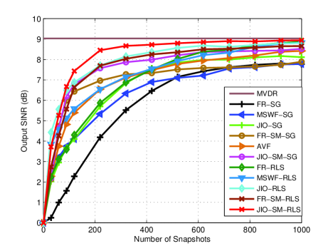
Figure 1: Output SINR versus the number of snapshots

The next simulation includes two experiments, which compare the proposed and existing algorithms with the time-varying and fixed bounds, respectively. The scenario is the same as that in Fig. 1. Fig. 2 (a) shows the results for the full-rank algorithms. We find that the FR-SM-RLS algorithm converges quickly to the steady-state with relatively low update rate ($\tau=20.5\%$). Due to the BPSK modulation scheme, it implies that the algorithm with the fixed bound $\delta=1.0$ should achieve a good performance. However, it requires more updates ($\tau=61.4\%$) and thus increases the computational cost. The curves with higher ($\delta=1.4$) or lower ($\delta=0.8$) bounds exhibit worse convergence performance. The same result can be found in Fig. 2 (b) for the reduced-rank algorithms. The proposed algorithm with the time-varying bound uses even less updates to realize a high output SINR performance.

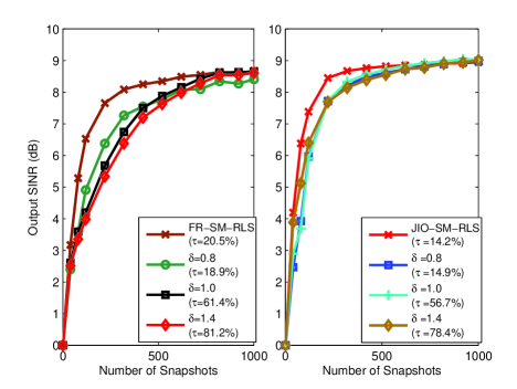
Figure 2: Output SINR versus the number of snapshots for (a) full-rank SM algorithms; (b) reduced-rank SM algorithms

VI Conclusion

We have introduced a new reduced-rank SM scheme and develop a RLS algorithm for implementation. The proposed scheme incorporates the SM mechanism with the time-varying bound into the reduced-rank JIO scheme to realize the data-selective updates of the full-rank and reduced-rank filters. The time-varying bound is combined in the LCMV optimization problem as a new constraint on the array output power to encompass the pairs of $\{\boldsymbol{T}_{r}(i),\bar{\boldsymbol{w}}(i)\}$ in the feasibility set of the proposed scheme. A RLS algorithm has been derived for implementation. The proposed algorithm achieves an improved performance with exchange of information between the projection matrix and the reduced-rank weight vector, reducing the computational cost primarily with the data-selective updates.

References

- [1] O. L. Frost, “An algortihm for linearly constrained adaptive array processing,” IEEE Proc., AP-30, pp. 27-34, 1972.
- [2] S. Haykin, Adaptive Filter Theory, 4rd ed., Englewood Cliffs, NJ: Prentice-Hall, 1996.
- [3] D. A. Pados and G. N. Karystinos, “An iterative algorithm for the computation of the MVDR filter,” IEEE Trans. Signal Processing, vol. 49, pp. 290-300, Feb. 2001.
- [4] M. L. Honig and J. S. Goldstein, “Adaptive reduced-rank interference suppression based on the multistage wiener filter,” IEEE Trans. Commun., vol. 50, pp.986-994, Jun. 2002.
- [5] R. C. de Lamare, “Adaptive reduced-rank LCMV beamforming algorithms based on joint iterative optimisation of filters,” Electronics Letters, vol. 44, pp. 565-566, Apr. 2008.
- [6] R. C. de Lamare and R. Sampaio-Neto, “Adaptive Reduced-Rank Processing Based on Joint and Iterative Interpolation, Decimation and Filtering”, IEEE Transactions on Signal Processing, vol. 57, no. 7, July 2009, pp. 2503 - 2514.
- [7] R. C. de Lamare, L. Wang, and R. Fa, “Adaptive reduced-rank LCMV beamforming algorithms based on joint iterative optimization of filters: Design and analysis,” Elsevier Signal Processing, vol. 90, pp. 640-652, Feb. 2010.
- [8] R.C. de Lamare, R. Sampaio-Neto and M. Haardt, ”Blind Adaptive Constrained Constant-Modulus Reduced-Rank Interference Suppression Algorithms Based on Interpolation and Switched Decimation,” IEEE Trans. on Signal Processing, vol.59, no.2, pp.681-695, Feb. 2011.
- [9] L. Guo and Y. F. Huang, “Set-membership adaptive filtering with parameter-dependent error bound tuning,” IEEE Proc. Int. Conf. Acoust. Speech and Sig. Proc., 2005.
- [10] P. S. R. Diniz, Adaptive Filtering: Algorithms and Practical Implementations, 3rd ed., Boston, MA: Springer, 2008.
- [11] L. Guo and Y. F. Huang, “Frequency-domain set-membership filtering and its applications,” IEEE Trans. Signal Processing, vol. 55, pp. 1326-1338, Apr. 2007.
- [12] R. C. de Lamare and P. S. R. Diniz, “Set-membership adaptive algorithms based on time-varying error bounds for CDMA interference suppression,” IEEE Trans. Vehicular Technology, vol. 58, pp. 644-654, Feb. 2009.
- [13] L. Wang, R. C. de Lamare, and M. Yukawa, “Adaptive reduced-rank constrained constant modulus aglorithms based on joint iterative optimization of filters for beamforming,” IEEE Trans. Signal Processing, vol. 58, PP. 2983 - 2997, June 2010.