Low Delay MAC Scheduling for Frequency-agile Multi-radio Wireless Networks

Abstract

Recent trends suggest that cognitive radio based wireless networks will be frequency agile and the nodes will be equipped with multiple radios capable of tuning across large swaths of spectrum. The MAC scheduling problem in such networks refers to making intelligent decisions on which communication links to activate at which time instant and over which frequency band. The challenge in designing a low-complexity distributed MAC, that achieves low delay, is posed by two additional dimensions of cognitive radio networks: interference graphs and data rates that are frequency-band dependent, and explosion in number of feasible schedules due to large number of available frequency-bands. In this paper, we propose MAXIMAL-GAIN MAC, a distributed MAC scheduler for frequency agile multi-band networks that simultaneously achieves the following: (i) optimal network-delay scaling with respect to the number of communicating pairs, (ii) low computational complexity of ${\mathcal{O}}(\log^{2}($maximum degree of the interference graphs$))$ which is independent of the number of frequency bands, number of radios per node, and overall size of the network, and (iii) robustness, i.e., it can be adapted to a scenario where nodes are not synchronized and control packets could be lost. Our proposed MAC also achieves a throughput provably within a constant fraction (under isotropic propagation) of the maximum throughput. Due to a recent impossibility result, optimal delay-scaling could only be achieved with some amount of throughput loss [30]. Extensive simulations using OMNeT++ network simulator shows that, compared to a multi-band extension of a state-of-art CSMA algorithm (namely, Q-CSMA), our asynchronous algorithm achieves a $2.5\times$ reduction in delay while achieving at least 85% of the maximum achievable throughput. Our MAC algorithms are derived from a novel local search based technique.

I Introduction

There are two emerging trends in the evolution of cognitive radio based wireless networks. First, new regulations allow the possibility for a single technology to utilize spectrum across very diverse range. For example, FCC mandated the use of unutilized TV spectrum in the $50\--698$ MHz band for unlicensed access [2]. Along with unlicensed spectrum in 2.4 GHz and 5.1 GHz, this implies that we now have fragments of unlicensed spectrum available across several GHz. Second, advances in RF technology allows cognitive radio based wireless devices to tune across large range of spectrum. For example, a recent product by Radio Technology Systems [3] makes it possible for radios to tune their center frequencies from 100 MHz to 8 GHz. Such radios are referred to as frequency agile radios. Note that, at any given time, the radio can tune to a single center frequency with a upper limit on the operating bandwidth (typically 40 MHz). These two trends imply that wireless devices have greater flexibility in adapting to the network. In this paper, we identify and address new challenges in MAC design that arise as a consequence of these trends.

We consider a wireless network where each network node is equipped with a cognitive radio that can detect the presence of a large number of available frequency bands. Since our work is on distributed MAC design, we implicitly assume that MAC has knowledge of available frequency bands; this knowledge could come from a layer/module that connects to a database or from a layer/module that connects to sensing equipments. The availability of frequency bands is quasi-static, i.e., the available frequency bands can change roughly at the time-scale of session durations and not at the time-scale of milliseconds. In the terminology of cognitive radio networks, the wireless network nodes are secondary transmitters and we assume that primary transmitters vacate the channels for large time-scales of the order of session durations. We also assume that each wireless node has potentially multiple transmitting radios to make full use of the cognitive capabilities. Each wireless node is allowed to transmit over all or a large subset of the detected frequency bands. For example, in a given location, the network codes can avail all unlicensed spectrum that could have 5 frequency bands consisting of 3 non-overlapping channels in 2.4 GHz ISM along with 2 TV whitespace bands $512\--524$ MHz and $692\--698$ MHz.

Thus, from a MAC design point of view, two aspects of cognitive radio capabilities of nodes are most relevant: firstly, multi-band RF capability of the radio nodes, and secondly, ability of a radio to switch frequency band with minimal switching overheads of less than millisecond [3]. While these provide additional flexibility for more efficient sharing of radio resources; however this also gives rise to new challenges in MAC scheduling. The key MAC scheduling question in such a network is: at every instant, which set of communicating node-pairs should operate over which frequency band and using which radio? Compared to traditional wireless networks, the MAC scheduling problem in cognitive radio based wireless networks is more complex due to two primary reasons:

1. Due to a potentially large number of available frequency bands, the number of feasible schedules increases considerably. Indeed, the number of available frequency bands can easily be few tens (e.g., $3$ non-overlapping frequency bands in 2.4 GHz, $13$ in 5 GHz, and another $5\--15$ frequency bands in TV whitespaces) in today’s networks. Thus, choosing the “right” schedule becomes computationally more challenging.

2. Since the available frequency bands can have diverse propagation characteristics, the interfering neighbors and the data rates depend on the operating frequency band. This is because wireless path loss inversely depends on the square of the operating frequency. This is unlike traditional wireless networks that operate either over a single frequency band or over multiple frequency bands with homogeneous propagation properties (referred to as multi-channel networks in the literature).

We wish to design practical and low-complexity MAC schedulers while addressing these unique challenges.

Design goal: While the MAC scheduling question can be answered differently depending on suitable performance goals, our primary objective is to minimize network queueing delay since network traffic is getting dominated by delay sensitive applications. Thus, we wish to design a MAC that meets the following simultaneous objectives: (i) low delay, i.e., total queueing delay scales linearly with the number of communication links which is the optimal scaling (ii) low computational complexity and protocol overhead, (iv) and very importantly, robust in the sense that it does not require nodes to be synchronized and allows for losses in control overhead. The reader might wonder why we do not mention maximizing network throughput as an objective. This is because, it has been shown in [30] that there is a fundamental trade-off between achieving 100% throughput, achieving delay that scales polynomially with the network size, and polynomial complexity of schedule computation, in the sense that all three cannot be achieved together. Thus, if we wish to design a low complexity scheduler that minimizes network delay, we must sacrifice on throughput. In this paper, we design a MAC scheduler that achieves our three objectives with minimal throughput loss.

Our approach: The theoretical underpinning of our work comes from so called local search based approaches for complex optimization problems. Local search is an iterative method, where, in each step, the current solution is improved by looking at the neighborhood of current solution. The choice of neighborhood of a feasible solution, along with how the transitions happen (it could be greedy, or random, or based on some transition probability structure) from one solution to another, determine the computational complexity and performance guarantee of the algorithm. Local search based algorithms are attractive due to their simplicity and amenability to distributed implementation. One popular local search based technique that has been applied to wireless scheduling problems is Glauber Dynamics based scheduling schemes and this is shown to achieve 100% throughput [24, 26, 14]. Referred to as Q-CSMA, these schemes are distributed and are computationally very light in each iteration (${\mathcal{O}}(1)$ computation time per iteration). However, convergence time of a Glauber Dyamics based scheme could be exponential in the size of the graph [9] which could adversely impact the network delay. Indeed, not much is known about delay guarantees of Glauber Dynamics based scheduling algorithms, except possibly for very special classes of network graphs (see Section II) in a single band scenario. The convergence issues of Glauber dynamics could exacerbate in multi-band cognitive-radio based wireless networks as the number of feasible schedules grows with the number of bands and radios. In this paper, we propose an alternative local search based distributed scheduling algorithm characterized by a very different solution-neighborhood and transition structure. Our scheme achieves optimal delay scaling in multi-band wireless networks but with at most ${\mathcal{O}}(1)$ fraction of throughput loss under isotropic propagation. Since it is impossible to achieve 100% throughput and optimal delay scaling simultaneously [30], our approach is complementary to Glauber dynamics based scheme; our scheme optimizes delay with some minimal loss in throughput, whereas, Glauber dynamics based scheme optimizes throughput and sacrifice on delay guarantees. Our scheme is distributed, requires ${\mathcal{O}}(\ln^{2}\Delta)$ ($\Delta$ is maximum degree of interference graph) computation time per schedule, and can be adapted to asynchronous setting.

Since MAC scheduling is a link-level decision, for simplicity and ease of exposition, we derive our scheme assuming all network traffic to be single-hop. We also describe later in the paper how all our results can be easily extended to a multi-hop network setting using a standard back-pressure based approach.

I-A Our Contributions

Our main contributions are as follows:

• Design of low-delay MAC scheduler for cognitive radio networks: First, for a synchronous network, we design a distributed scheduling (called the MAXIMAL-GAIN algorithm) algorithm that provably achieves all of the following: (i) an average network-wide total queue length that scales as $HM$ where $H$ is the number of transmit-receive pairs and $M$ is the number of available frequency bands, (ii) computational overhead ${\mathcal{O}}(\log^{2}\Delta)$ times the time required to exchange RTS-CTS message between two neighboring nodes (here $\Delta$ is the maximum degree of the network graph), and (ii) any throughput within a factor $\beta$ of the throughput region where $\beta$ is a topology dependent parameter that is ${\mathcal{O}}(1)$ for practical networks like grid, hexagonal deployment, random deployment with isotropic propagation etc.

• Developing extensions for asynchronous network: In an asynchronous cognitive-radio based wireless network, we identify several issues that can severely impair the performance of scheduling algorithms developed for synchronous setting. Inspired by the design philosophy of the synchronous MAXIMAL-GAIN algorithm, we design a robust MAXIMAL-GAIN like CSMA based algorithm for asynchronous settings.

• Evaluation: We provide detailed evaluation of our algorithm. To evaluate the benefits of designing a delay-centric MAC and to understand the throughput-loss of our MAC, we compared our algorithm with a multi-band multi-radio adaptation of a distributed and practically implementable MAC that is known to achieve 100% throughput (namely, Q-CSMA [24]). We compared the asynchronous version of our algorithm with Q-CSMA which is synchronous in nature. We report results of extensive simulations over the OMNet network simulator. We show that our MAXIMAL-GAIN algorithm achieves $2\--3\times$ reduction in delay, while achieving over $85\%$ of the maximum possible throughput.

II Related Work

The extensive research on MAC scheduling in single band networks (see [20] for an excellent survey) can be broadly divided into two classes: max-weight computation based and Glauber dynamics based. The first class of approach is inspired by the seminal work [33] which proves that maximum-weight (MW) scheduling achieves 100% throughput. The MW scheduler MAC activates at every instant a non-interfering set of links such that the total of weighted data-rates of the activated links is maximized, where, weight of a link is roughly defined by the number of backlogged packets. Furthermore, a recent work [18] (also see [23, 22]) has shown that an MW schedule achieves order optimal delay scaling with the number of links. However, computing MW schedule is NP-hard, leading to considerable research on approximate MW schedules [32, 21, 28, 19]. However, extending these works to multi-band wireless networks, with distributed implementation and low complexity, is not easy. As discussed in Section I, the second class of approach [24, 26, 14] is motivated by so called Glauber dynamics based local search. These scheme achieve 100% throughput but do not provide delay guarantees in general networks.

Some examples of work that focus on low delay algorithms in single band networks are [15, 12]. For single band networks, low delay CSMA based algorithms for special classes of interference graphs have been proposed: [29] proposes a delay-optimal CSMA based MAC for polynomial growth networks (i.e., the number of nodes $r$ hops away from a node is polynomial in $r$), and [13] proposes polynomial delay Q-CSMA based algorithm for bounded degree networks.

Multi-radio multi-channel resource allocation is addressed in [34, 16, 21]. Unlike our work, none of these works account for the fact that different bands can have different propagation characteristics.

The inspiration of our MAC comes from application of local search based techniques to develop approximation algorithms for NP-hard optimization problems. We refer the reader to [5] for an excellent survey.

III Preliminaries

III-A Network Model

We consider a wireless network with ${\mathcal{V}}$ as the set of nodes. The radio resources available are multiple frequency bands with diverse propagation characteristics. By frequency band, we mean a contiguous slice of spectrum of width at most $B_{max}$, the maximum tunable range of a radio. If there is a larger contiguous band $W$ available, we split it into “bands” of equal width $B_{max}$, with the last band having width possibly less than $B_{max}$. Since the frequency bands have diverse propagation, the data rate between a transmitter-receiver pair in the network and the interfering neighbors of the transmitter-receiver are frequency dependent. The availability of frequency bands do not change for the duration of a session. In the terminology of cognitive radio networks, the wireless network nodes are secondary transmitters and we assume that primary transmitters vacate the channels for large time-scales of the order of session durations.

Each network node has cognitive radio capabilities by which we mean the following:

1. Each wireless node has $K$ half-duplex radios capable of tuning across a large frequency range (e.g., from 100 MHz to 2.5 GHz, [10]). Each node can detect and communicate over all the frequency bands. This model subsumes the case where a node can only detect/use a subset of the available bands by setting the PHY data rates (we will elaborate on this later in the section) over the prohibited frequency bands to be zero. We also remark that our work easily generalizes to the case where different mesh nodes have different number of radios.

2. We assume that at any given time any radio can tune to only a single frequency band (e.g., 500MHz, 2.4GHz etc.) and the bandwidth can range from 0 to $B_{max}$.

We consider all traffic between one-hop communication pairs which is a standard approach to designing a MAC scheduler. Since MAC scheduling is a link level decision, the single hop setting is not limiting at all and the extension to a multi-hop setting can be done in a standard manner [33] using queue back-pressure based approach (see Section IV-D for the required modifications). Towards this end, we will denote by ${\mathcal{H}}$ the set of single-hop node pairs and let $\lvert{\mathcal{H}}\rvert=H$. Since we are considering a multi-band wireless network, we call a node pair $(u,v)$ single hop if $u$ can transmit to (or receive from) $v$ at non-zero rate over at least one of the available bands. We consider a slotted system. Associated with each single hop node pair $h\in{\mathcal{H}}$ is a stochastic arrival process $\{A_{h}(t)\}$, where $A_{h}(t)$ is the number of packets arriving to node pair $h$ in time-slot $t$. Let $\lambda_{h}=E[A_{h}(t)]$ be the average arrival rate at node pair $h$. We will also assume that the arrival processes have bounded second moments. We will assume that the arrival process is i.i.d. across time slots. Let $D_{h}(t)$ be the number of packets that depart from node pair $h$ in time-slot $t$ and let $q_{h}(t)$ be the queue length at the end of time-slot $t$. We will assume that the arrivals happen at the beginning of the slot. The queue length evolution can be described by

$$q_{h}(t+1)=[q_{h}(t)+A_{h}(t)-D_{h}(t)]^{+}\ .$$

We will also refer to $\Lambda$ as the set of all possible arrival rate vectors that can keep the queues bounded for some sequence $\{D_{h}(t)\}_{t}$ that is feasible. The arrivals are also assumed to have bounded second moments.

Transmission over a node-pair can happen at different rates depending upon the frequency band it is operating on. We next extend the standard definition of link (and associated link data rate) between any node pair to account for the frequency band dependent data rate.

Network graph and generalized link

We assume that the spectrum available in the system is fragmented and spans a large range (e.g., 50-700MHz, 2.4GHz and 5.2GHz). Let $M$ be the number of frequency bands. We will also assume that the bands are ordered in the real axis from left to right, and we will simply say band $f_{j},\ j=1,2,\ldots,M$ to mean the ${j}^{\text{th}}$ frequency band. We will also use “band-$j$” and “frequency band $f_{j}$” interchangeably.

Radio propagation physics dictates that, if all other parameters remain same, the received signal strength at a receiver is inversely proportional to the square of the carrier frequency [27] (i.e., halving the frequency doubles the received signal strength). Thus, it is possible that two nodes in the network may be able to communicate on a frequency band $f_{1}$ but unable to communicate on frequency $f_{2}$.

The network connectivity in frequency band-$j$ is modeled as a graph $G_{j}({\mathcal{V}},{{\mathcal{E}}}_{j}),j=1,2,\ldots,M$ where ${\mathcal{V}}$ is the set of network nodes and for two nodes $u$ and $v$, $(u,v)\in{{\mathcal{E}}}_{j}$ if $u$ can communicate with $v$ over frequency band $f_{j}$ at a non-zero data rate. Also, we will denote by $\Delta_{j}$ the maximum degree in the graph $G_{j}({\mathcal{V}},{{\mathcal{E}}}_{j})$ and $\Delta=\max_{j}\Delta_{j}\ .$

Definition 1 (Generalized link).

A generalized link is defined by (i) the band $m$ over which the link exists, and (ii) the ordered node-pair $(i,j)$ to indicate that node $i$ is the transmitting node of the link and $j$ is the receiving node of the link (more precisely, one of the radios of node $i$ ($j$) is the transmitting (receiving)). We will also use the notation $\text{band}(l)=m,\ \text{head}(l)=j,\ \text{tail}(l)=i$ to describe link-$l$.

Remark 1.

Our algorithms use the notion of generalized link that abstracts out diverse propagation in different bands. Indeed, there could be multiple generalized links between two nodes each corresponding to different bands with different data rates and different interference neighborhoods.

In the rest of the paper, we say link to mean generalized link. Note that, multiple links can exist between two nodes if they can communicate at non-zero rate over multiple frequency bands. We denote the data rate over generalized link-$l$ by $r_{l}$. We define the weight of a generalized link $l$, $w_{l}$, as follows.

Definition 2 (Weight of a link).

We define the weight of link $l$ as $w_{l}=q_{h}$, if link $l$ is on hop $h\in{\mathcal{H}}$, i.e., $w_{l}$ is the queue backlog on hop $h$.

Interference model

Our interference model is the widely used secondary interference [31, 6, 20] model. In this model, two links $l_{1},l_{2}$ interfere over a frequency band $f_{j}$ if any one of the end points of $l_{1}$ can decode messages from any one of the end points of $l_{1}$ even at the lowest possible modulation and coding. Such an interference model is essential for the functioning of RTS/CTS based CSMA algorithm.

Thus, each generalized link-$l$ has a set of interfering links denoted by $I_{l}$. Thus, if $l^{\prime}\in I_{l}$, $l$ and $l^{\prime}$ cannot transmit simultaneously. Note that the notion of generalized links easily accounts for the fact that the interfering node-pairs of a node-pair can be different in different bands. To keep the exposition focused, for now and unless stated otherwise, we ignore adjacent channel interference (ACI) (due to imperfect RF hardware causing transmit power to leak into adjacent bands) in multi-band networks [8]. In Section IV-D, we outline how our model, algorithm, and analysis can be easily adapted to account for ACI.

Some of the useful notations are shown in Table I.

TABLE I: Table of Notations

$M$	Number of available frequency band
$f_{j}$	Frequency band indexed $j,\ j=1,2,\ldots,M$
${\mathcal{V}}$	Set of mesh nodes; $\lvert{\mathcal{V}}\rvert=V$
${\mathcal{E}}_{j}$	Set of connected node pairs in $f_{j}$
${\mathcal{H}}$	Set of single-hop
	source destination pairs; $\lvert H\rvert=H$
$\mathcal{L}$	Set of links, $\lvert\mathcal{L}\rvert=L$
head($l$) and	Receiving and transmitting
tail($l$)	node of link $l$.
band($l$)	Frequency band of link $l$.
$r_{l}$	Data rate of generalized link $l$
$I_{l}$	Set of links that interfere with link $l$
	(the interfering links belong to band($l$).)
$w_{l}$	Weight of generalized link $l$ ($w_{l}=q_{h}$
	if $l$ is a link between $h$ node-pair)
$S_{t}$	Set of activated links under
	MAXIMAL GAIN schedule at time-slot $t$
$S_{t}(f_{j})$	Set of activated links over band $f_{j}$
	in MAXIMAL GAIN schedule at time-slot $t$

Some useful definitions

Finally, we provide a few useful definitions. Using standard definition, we say $I\subseteq{\mathcal{V}}$ is independent set of a graph $G({\mathcal{V}},{\mathcal{E}})$ if no two vertices in $I$ share an edge.

Definition 3 (2-hop neighborhood MIS cover).

The 2-hop neighborhood maximum independent set (MIS) cover of a vertex $v$ (denoted by $\kappa_{j}(v)$) in a network graph $G_{j}({\mathcal{V}},{{\mathcal{E}}}_{j})$ over frequency band $f_{j}$ is defined as the maximum size of an independent set in the graph induced by the nodes that lie within 2 hops of $v$ in $G_{j}({\mathcal{V}},{{\mathcal{E}}}_{j})$. We also define 2-hop neighborhood MIS cover of $G_{j}({\mathcal{V}},{{\mathcal{E}}}_{j})$ as $\kappa_{j}=\max_{v\in V}\kappa_{j}(v).$

Finally, we will use the standard definitions of interference degree in [6, 20], throughput optimality and stability region [20]. Denote by $\mathcal{S}$ the set of all feasible schedules.

Definition 4 (Interference degree).

The interference degree of link $l$ is defined as the maximum number of links that can be activated simultaneously over band($l$) in a schedule. We will denote the interference degree of link $l$ as $\beta_{l}$ and we also define the interference degree of the network as $\beta_{max}=\max_{l}\beta_{l}$.

Definition 5 (Stability region and throughput optimality).

The stability region $\Lambda$ is the set of all arrival rates $\lambda$ such that $\lambda=\sum_{i}\phi_{i}S_{i},S_{i}\in\mathcal{S}$ for some ${\phi_{i}}$, with $1\geq\phi_{i}\geq 0,\forall i$ and $\sum_{i}\phi_{i}=1$.

An algorithm which stabilizes (the queues remain bounded) all arrival rates $\lambda\in\Lambda$ is said to be throughput-optimal. An algorithm which stabilizes all arrival rates $\lambda\in\frac{\Lambda}{\mu}$, for some $\mu>1$ is said to be a $\mu$-factor throughput-optimal algorithm.

III-B Scheduling Problem

The scheduling problem we consider is to activate a set $S_{t}$ of generalized links at each time $t$, so that the set of activated links satisfy the following constraints.

• Interference constraint (SI): As we described earlier in this section, this states that, if $l$ is activated no link in the interference neighborhood $I_{l}$ can be activated. The secondary interference constraint along with our notion of generalized link also captures the following important constraint in multi-band networks: if a node $v$ is involved in communication with node $u$ over frequency band $f_{j}$ over a radio, no other node can communicate with $v$ over $f_{j}$ at the same instant.

• Maximum Radio Constraint (MR): Since there are $K$ radios at a node, at a time, there can be at most $K$ active links that are part of a node with each link belonging to distinct bands.

Our goal in this paper is to derive a distributed scheduling algorithm, that has the following properties.

(P1.) Low Complexity: The schedule computation complexity should be independent of the overall network size, number of available bands $M$ and number of radios $K$. Since this requirement is too stringent, we relax this slightly to allow the complexity to have poly-logarithmic dependence on the maximum degree but independent of $M$, $K$, and overall network size.

(P2.) Optimal delay scaling: The scheduling policy should provide an order-optimal delay guarantee of $E[Q_{tot}]={\mathcal{O}}(H)\ ,$ where $Q_{tot}$ is the total queue length in the entire network. Note that the requirement of delay to grow linearly with number of single-hop pairs is stronger than requiring the delay to be polynomial in the network size.

(P3.) Minimizing throughput-loss: We want our algorithm to be a $\mu$-factor throughput optimal (see Definition 5) algorithm, where $\mu\geq 1$. This is motivated by the fact that, achieving the delay scaling in P2 with a polynomial algorithm is bound to result in some loss in throughput [30]. We will propose MAC such that $\mu$ is an universal constant under an isotropic propagation model in every frequency band.

IV Synchronous MAXIMAL-GAIN

We now propose our local search based algorithm. In this section, we will assume that the nodes are synchronized; in a subsequent section, we show how our algorithm can be adapted to asynchronous setting.

In the rest of this section, we assume a time-slot based system. Nodes are synchronized and each time-slot has two phases: schedule computation phase and data transmission phase. Our focus is on the schedule computation phase. The schedule computation phase is further divided into a certain number of mini-slots over which schedule is computed. The duration of each mini-slot is just long enough for one round of RTS-CTS message exchange.

IV-A Intuition and Algorithm Overview

A local search based algorithm has the following underlying principle: the solution iteratively moves from one state (i.e., feasible solution) to another neighboring state such that the new state provides improvement in the objective. The challenge often lies in appropriate definition of neighborhood-states of every state (the neighborhood of different states can overlap), such that the algorithm achieves the desired goals of distributed implementability, fast convergence, and provable approximation to the optimum. In our case, there is an additional challenge arising from the fact the weights (queue-lengths) are dynamic quantities.

To aid our discussion, we first introduce a few notations. First of all, we say “link $l$ is active in $S$” to mean “link $l$ is a part of schedule $S$.” For any feasible schedule $S$ (defined by a set of non-interfering (generalized) links), we will denote by $S(f_{j})$ as the set of active generalized links in $S$ over frequency band $f_{j}$. Clearly, $S=\cup_{j}S(f_{j})$. Also, let $S_{t}$ be a feasible schedule at time $t$. Note that, feasibility of $S_{t}$ also means that no node has more than $K$ (number of radios) active links. We use the terms “state” and “feasible schedule” interchangeably. Towards developing a local search based algorithm, we first define our notion of neighboring states.

Neighborhood states: Let $H_{1},H_{2},H_{3}\ldots$ be a disjoint partition of all nodes ${\mathcal{V}}$ with the following two properties: (i) the sub-graph of $G_{1}({\mathcal{V}},{\mathcal{E}}_{1})$ (the network graph is the lowest frequency band) induced by $H_{k}$ has a star-subgraph containing all nodes in $H_{k}$, i.e., there is a node $u_{k}$ (called star-center or leaders) that can communicate with all other nodes in $H_{k}$, (ii) the star-centers of $H_{1},H_{2},H_{3},\ldots$ form an independent set in $G_{1}({\mathcal{V}},{\mathcal{E}}_{1})$. Figure 1 illustrates this partition. The reason for such a partition will become clear soon. We will refer to each $H_{k}$ as a group. For a feasible schedule $S$, let $S^{H_{k}}$ be the set of active links in $S$ outgoing from some node in group $H_{k}$, i.e., $S^{H_{k}}=\{l\in S:\text{tail}(l)\in H_{k}\}$. A feasible schedule $S^{\prime}$ is a neighboring state of another schedule $S$, if, for each $k$, there is at most one frequency band where ${S^{\prime}}^{H_{k}}$ has additional active links compared to $S^{H_{k}}$. More precisely, $S^{\prime}$ is a neighbor of $S$, iff, for each $k$, all generalized links belonging to set ${S^{\prime}}^{H_{k}}\setminus S^{H_{k}}$ operate over the same frequency band. We will denote by $\text{nghbr}(S)$ the neighboring states of a state $S$.

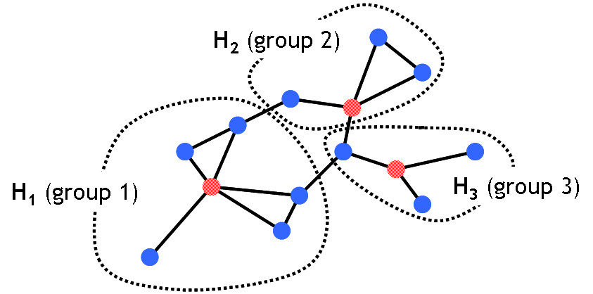
Figure 1: Illustration of partitioning the network graph $G_{1}({\mathcal{V}},{\mathcal{E}}_{1})$. Each group has a star-subgraph containing all nodes in group; red (shaded) nodes are star-centers (leaders).

Overview of the algorithm: In each time-slot, our MAC chooses a new schedule by performing a single iteration of local-search. Given a partitioning of ${\mathcal{V}}$ into $H_{1},H_{2},\ldots$ and our definition of $\text{nghbr}(S)$, the high-level steps of our MAC algorithm are as follows.

1. Random Selection of Bands: Because of our definition of neighboring states, for any group $H_{k}$, a new schedule can activate additional links in at most one frequency band. In this step, each group independently chooses a frequency band at random; this random frequency band is used for activating new outgoing links from $H_{k}$. Of course, instead of choosing a band at random, another option could be to choose a frequency band that yields maximum improvement in the total weight over the current schedule. However, such a operation can incur significant overhead and will have computational and messaging complexity ${\mathcal{O}}(M)$. We show that, random selection of a band just works fine.

2. Computing maximum improvement links: Once a frequency band is chosen at random for every group $H_{k}$, the next step is to find a link/s whose activation over this band results in maximum improvement in the total weight of all links outgoing from $H_{k}$. We will call these links high-priority links. Note that, if a new link is activated, some other links may have to be deactivated (removed from the existing schedule) for the new schedule to be feasible.

3. Computing schedule: Observe that, the new high priority links cannot be activated all at once as some of them could interfere with each other. This final step computes a new feasible schedule by only selecting a non-interfering sub-set of high-priority links. This selection can be performed using CSMA-CA or any standard random access protocol (in every band) among the high priority nodes. All non-high priority links continue transmission only if no high-priority link can be sensed.

So far we have just provided an overview of the algorithm, the above steps also have to be performed in a distributed manner. In Algorithm I, we show the precise details of how this can be done.

Remark 2 (Compelxity).

The complexity of schedule computation is dominated by distributed computation of the maximum gain link in every group. As we describe in Section IV-B, this can be performed in ${\mathcal{O}}(\ln^{2}\Delta)$ mini-lots (the duration of mini-slot is long enough to exchange an RTS-CTS message) which is essentially the time-complexity of schedule computation.

   

Algorithm I: Algorithm Maximal-Gain Schedule

1:  Grouping and initialization (one time operation at time-$0$): At time-$0$, the nodes are partitioned into groups and initialized using the following steps:

1. Use any known distributed computing algorithm (e.g.  [25]) to compute an independent dominating set. $D$ in the graph $G_{1}(V,E_{1})$. Nodes in $D$ are called leaders.

2. Every node not in $D$ becomes a follower of any one neighboring leader. A leader along with all its followers are referred to as a group. Let $H_{1},H_{2},\ldots$ denote the groups.

3. All nodes in a group choose a common seed for random number generation.

2:  for all time-slots $t$ do

3:     Every node uses the seed common to its group to select a frequency band uniformly at random from the $M$ available bands.

4:     Gain computation by nodes: Every node $v$ computes the gain in total weight of outgoing links from $v$ if some outgoing link from $v$ were activated over the randomly selected frequency band. Denoting the randomly selected band for node $v$ as $f(v)$, this computation is as follows:

1. For every node $v$, if a new outgoing link from $v$ were to be activated over $f(v)$, some link $l^{\prime}$ may have to be deactivated to maintain the feasibility of the new schedule. This link $l^{\prime}$ (with $v$ as one end) is any link that is active over band $f(v)$ in schedule $S_{t-1}$; if no such link exists in $S_{t-1}$, but all $K$ radios of $v$ are used up in $S_{t-1}$, then $l^{\prime}$ is the one with the minimum value of $w_{l}r_{l}$. If there is such an $l^{\prime}$, then $v$ computes $loss(v)=w_{l^{\prime}}r_{l^{\prime}}$ based on the above; else $loss(v)=0$.

2. The net gain due to node $v$ activating a link over band $f_{j}$ is computed as follows.

   $$gain(v)=\max_{\{l:\text{tail}(l)=v,\text{band}(l)=f_{j}\}}\left(w_{l}(t)-loss(v)\right)^{+}$$ (1)

5:     Computing maximum gain link in every group: Every group computes the outgoing link in that group with the maximum gain in a distributed manner. In Section IV-B, we show that, this can be done with minor modifications in CSMA protocol in ${\mathcal{O}}(\ln^{2}\Delta)$ mini-slots where a mini-slot is the time taken to exchange a pair of RTS-CTS message between communicating nodes. At the end of this step, every node knows which, if any, of its outgoing link has maximum gain. These nodes are termed high-priority nodes.

6:     Contention resolution among high-priority nodes: Finally, the high-priority nodes perform CSMA like contention resolution in their selected frequency band. All other nodes that are not high priority, but were active in $S_{t-1}$, continue their transmission only if they do not sense the channel to be occupied by a high-priority node (this is inferred by listening to RTS/CTS in the contention resolution phase.)

7:  end for

 

IV-B Computing Maximum Gain in a Group

In the description of MAXIMAL GAIN Algorithm, we have assumed that, each group can compute the maximum gain in the group in $T_{comp}={\mathcal{O}}(\ln^{2}\Delta)$ mini-slots. Recall that, these mini-slots belong to schedule computation phase of a slot. We now adapt binary search for a broadcast environment to achieve this.

We first argue that, it is sufficient to prove the result by assuming that broadcast messages from nodes in any group do not collide with that of other groups. To see this, suppose we assign color to each group so that any two groups that have interfering nodes are not assigned the same color. Under isotropic propagation, simple geometric considerations show that $\chi={\mathcal{O}}(1)$ colors suffice. Thus, we can color-code the mini-slots in a round-robin manner and allow each group to perform the steps of max-computation only in mini-slots corresponding to its color. Thus, if each group requires $T_{comp}$ mini-slots, the overall computation would require $\chi T_{comp}={\mathcal{O}}(T_{comp})$ mini-slots. Note that, the coloring is a one-time procedure that can be done in a distributed manner at the beginning of network operation.

The following simple procedure computes the maximum-gain link in a group in $T_{comp}={\mathcal{O}}((\ln\Delta)^{2})$ mini-slots.

 LOCAL MAX: Computing maximum gain in a group  

Each group is isomorphic to a start graph. We will call the start-center as group leader and every other node as follower. Suppose $N_{v}$ is the number of nodes in a group to which node $v$ belongs. Gain of a node is given by (1).

• Step 1: Initially every follower node with positive gain is a candidate winner node. Initialize broadcast probability of every node $v$ with positive gain as

  $$p_{bc}(v)={\textstyle{\frac{1}{2N_{v}}}}$$

• Step 2: In the next mini-slot, with probability $p_{bc}(v)$, a follower $v$ sends an RTS message containing its gain (say the value is $g$). If there are no collisions, the group leader sends a CTS echoing the gain.

• Step 3: In case of CTS, all follower nodes with equal or lower gain than $g$, remove them from the list of candidate winners.

• Step 4: Once every $C_{1}(1+\ln(N_{v}))$ mini-slots, every candidate node $v$ updates $p_{bc}(v)$ as

  $$p_{bc}(v)\leftarrow 1.5p_{bc}\ .$$

  Here $C_{1}$ is a positive constant.

• Step 5: Step 2-4 are are repeated with the remaining candidate winners for $C_{2}\ln(N_{v})(1+\ln(N_{v}))$ mini-slots, where $C_{2}$ is a positive constant.

 

Lemma IV.1.

Suppose we choose $C_{1}=1/\ln(9/8)$ and $C_{2}=C_{1}/\ln(1.5)$. Then, Procedure LOCAL MAX computes the maximum gain in a group in $T_{comp}={\mathcal{O}}(\ln\Delta)^{2}$ mini-slots with probability at least $1/2$, where $\Delta$ is the maximum degree of the communication graphs over all bands..

Proof.

See the longer version [7]. ∎

IV-C Throughput and Delay Guarantee

The following result states the throughput and delay guarantee of MAXIMAL-GAIN scheduling algorithm in terms of the graph-parameters $\kappa_{1}$ and $\beta_{\max}$ defined in Section III.

Theorem 1.

The MAXIMAL-GAIN Algorithm has time-complexity of ${\mathcal{O}}((\ln\Delta)^{2})$ times the time required to exchange an RTS-CTS message between two neighbors. The algorithms provides the following guarantees:

• MAXIMAL-GAIN algorithm stabilizes all arrival rate vectors $\lambda$ such that $\lambda\in\frac{\Lambda}{\mu},$ where

  $$\mu=\beta_{\max}(1+2(1+\kappa_{1}))\ .$$ (2)

• If $\lambda+\epsilon\in\Lambda/\mu$ for some $\epsilon>0$, then the total queue length achieved by the MAXIMAL-GAIN algorithm, $Q_{tot}(t)=\sum_{h}q_{h}(t)$ satisfies

  $$\lim\sup_{T\to\infty}\frac{1}{T}\sum_{t=0}^{T-1}E[Q_{tot}(t)]=\frac{c_{1}\ MH}{\epsilon},$$

  where $c_{1}$ is a universal constant independent of the network parameters and radio resources.

The proof is relegated to the Appendix.

Remark 3 (On total queue length bound).

Part (ii) of Theorem 1 can also be stated in terms of offered load $\rho<1$. Suppose $\lambda\in\rho\Lambda$. Then under mild technical conditions (see Proposition 4, [18]) that hold for most practical topologies, one can choose $\epsilon=c_{2}(1-\rho/\mu)$ for network independent constant $c_{2}$, and thus leading to a total queue-length bound of ${\mathcal{O}}(MH/(1-\rho/\mu))$.

Remark 4 (On the proof of Theorem 1).

Since we perform a single iteration of local search in each time-slot, each subsequent iteration of local search is with a modified weight (queue-length). The main technical contribution of the proof is in showing that our local search based algorithm converges even though the weights (or queue-lengths) are changing dynamically. This is unlike Glauber Dynamics based local search where the weights must be a slowly-changing function of queue-length for convergence to happen [26].

Remark 5 (Refinements of Theorem 1).

The results of Theorem 1 can be further refined as follows:

1. Suppose the MAXIMAL-GAIN algorithm repeats the randomized algorithm for computing LOCAL-MAX $\ln(1/\epsilon)/\ln(2)$ times so that the maximal gain in a group is computed with probability at least $1-\epsilon$ instead. Then, the achievable throughput region in Theorem 1 improves to $\Lambda/\mu^{\prime}$ where

   $$\mu^{\prime}=\beta_{\max}(1+{\textstyle{\frac{1+\kappa_{1}}{1-\epsilon}}})\ ,$$ (3)

   and time complexity of the algorithm becomes ${\mathcal{O}}((\ln\Delta)^{2}\ln(1/\epsilon))$ times the time required to exchange an RTS-CTS message between two neighbors.

2. We have stated Theorem 1 simply in terms of generic graph parameters. However, we can provide improved bound in terms of one-time grouping that we perform. Precisely, let the grouping be such that any generalized link is interfered by links from at most $\sigma$ distinct groups other than its own group. Then, combined with $\ln(1/\epsilon)/\ln(2)$ repetitions of randomized LOCAl-MAX, the achievable throughput region in Theorem 1 improves to $\Lambda/\mu^{\prime\prime}$ where

   $$\mu^{\prime\prime}=\beta_{\max}(1+{\textstyle{\frac{1+\sigma}{1-\epsilon}}})\ .$$ (4)

   Thus, if the one-time grouping can be performed efficiently so that $\sigma$ is low, then the bounds can be much better.

IV-C1 Performance guarantee for special cases

Using Theorem 1 and refinements in Remark 5, we can show that he throughput guarantee can be bounded by a constant for many practical networks:

• Example 1. Under isotropic propagation, simple geometric considerations show that the 2-hop neighborhood MIS cover is a constant independent of network parameters, i.e., $\kappa_{1}={\mathcal{O}}(1)$. Along with the fact that the interference degree, $\beta_{max}$ is a constant under isotropic propagation, the throughput loss of MAXIMAL-GAIN schedule is at most ${\mathcal{O}}(1)$ fraction of full throughput.

• Example 2. In a linear chain or ring based network graph, the throughput guarantee is $1/8$ (using (4)) of the maximum throughput. Assuming efficient grouping, same bound holds for a network formed by combining several linear chains where the nodes from two different chains interfere only where the chains intersect. This kind of network is representative of infrastructure based wireless networks deployed by placing nodes along city roads.

• Example 3. For tree graphs such that the tree junctions are at least 2-hops away, the throughput guarantee can be shown to be within around $1/8$ of maximum throughput if the set of group leaders include all tree junctions.

In Section VI, we show that the actual throughput guarantee of MAXIMAL-GAIN is much better in practice for random topologies and grid. In fact, in all our evaluations even under asynchronous setting, we found that the throughput loss of our algorithm is never more than $20\%$.

IV-C2 Comparison with other algorithms

It is instructive to compare the theoretical performance of our algorithm with two popular algorithms: greedy maximal scheduling (GMS) [20, 19] and Q-CSMA [24, 26, 14] across three important measures: complexity, throughput, and delay. Our algorithm has a throughput guarantee factor $\mu=\beta_{\max}(1+2(1+\kappa_{1}))$ that has two multiplicative terms: a term $\beta_{\max}$ arising due to greedy computation of maximal gains link within a group, and a term $(1+2(+\kappa_{1}))$ arising due to contention resolution among winner links of different groups. The second term is essential due to grouping mechanism which is key to making our algorithm distributed with a complexity that simply scales as ${\mathcal{O}}((\ln\Delta)^{2})$ which is independent of the network size. On the other hand, greedy maximal scheduling (GMS) [20, 19] adapted to our setting has a throughput guarantee factor of $\beta_{\max}$ and provides optimal throughput scaling as with our algorithm. However, the price of GMS is in terms of much higher computational complexity. Indeed, even a distributed implementation of greedy maximal schedule could easily require $\Omega(MH\log(MH))$ mini-slots [20] and this could be difficult to implement even for moderate values of number of bands ($M$) and number of hops ($H$). Thus, the $\kappa_{1}$ dependent second term in our performance guarantee can be viewed as the cost of distributed implementability with a complexity that is practically independent of network size and fully independent of number of bands. Finally, Q-CSMA or Glauber Dynamics based algorithm when applied to our setting would provide a throughput of 100% and distributed-complexity that is essentially ${\mathcal{O}}(1)$; however, the price of such an algorithm is that total queue length is not guaranteed to be even polynomial in the network parameters like number of nodes, bands etc. Thus, our algorithm strikes a trade-off between distributed-complexity, throughput, and delay guarantee by simultaneously guaranteeing bounded throughput loss, network independent distributed complexity, and linear (in number of hops) delay scaling. Our evaluation in Section VI using multi-band asynchronous versions of the algorithms show that, throughput of MAXIMAL-GAIN is typically within 80% of throughput of Q-CSMA and almost on par with GMS, and average delays are considerably better than both Q-CSMA and GMS.

IV-D Extensions

Extensions to account for ACI: Due to leakage in adjacent frequency band caused by non-ideal filters in transmitters, interference can be also caused by radios transmitting in adjacent frequency band [8]. We can account for this by defining the interfering links $I_{l}$ to be a union of links causing secondary interference and links causing ACI. Some minor modifications are required in the local computation of gain in MAXIMAL GAIN scheduler. We skip the details.

Extensions to multi-hop setting: Our algorithm can be extended to a multi-hop setting by choosing the weights using “queue back-pressure” mechanism developed in [33]. Essentially, instead of choosing the weights as queue-lengths, they must be chosen as differential queue-length as compared to next hop. Some minor changes are required to ensure that nodes can learn suitable information from the neighborhood to compute the queue back-pressure based weights.

V Asynchronous Maximal-Gain

We now use the design philosophy of synchronous Maximal-Gain algorithm to develop a distributed MAC scheduler for wireless networks where nodes could be asynchronous or where control packets could be lost. Since the asynchronous model is difficult to analyze without further assumptions, we will provide simulation evaluation of this asynchronous MAC in Section VI.

Due to multi-radio multi-band setting, there are two key challenges in extending our synchronous MAC to an asynchronous setting. First, since there are fewer radios (per node) than bands in a typical setting, it is difficult for nodes to keep track of activities and availabilities of different bands. Second, nodes in a group may not have up to date information on the maximum-gain link.

To alleviate the first problem, we assume that each wireless node has one extra radio for exchange of control messages on a dedicated control band which is a standard approach [17]. All nodes use the control band to send RTS/CTS messages to reserve an intended band (the intended band is decided using our algorithm described shortly). To alleviate the second problem, we use the design philosophy of synchronous Maximal-Gain scheduler as follows. Recall that in the synchronous Maximal-Gain algorithm, in each scheduling slot, each group does the following: (i) choose a band at random and (ii) the maximum-gain link contends for channel access in the chosen band. This can be viewed as assigning priorities to (generalized) links as follows: any maximum-gain link in a randomly picked band has highest priority (HP), the links that transmitted in the previous transmission opportunity but has no HP link in the interference neighborhood, have medium priority (MP), all other links have low priority (LP) and can transmit only if no HP and MP links contend. The prioritization of the links can be achieved by allowing links of different priorities to contend in different parts of contention window as described shortly.

With the above intuition, we now describe our asynchronous MAC scheduler. In the following, we assume that the grouping of the nodes is done identical to that described for the synchronous algorithm. The star-centers are called leaders and they have some extra functionalities. Later in this section, we describe a method to eliminate the role of a leader.

 The Asynchronous MAXIMAL-GAIN Algorithm  Leader’s algorithm: The leader in each group performs two key functions: maintaining, updating, and broadcasting information about the group members, and selecting the maximum-gain link dynamically.

• Information update: All nodes send RTS/CTS messages over the control band for an intended link (the choice of the intended link is described later in the algorithm). Any RTS/CTS message contains the following: (i) queue-length information of the intended link, (ii) the frequency band of the intended link, (iii) and the data rate of the intended link. Whenever a leader hears an RTS/CTS message from a group member over the control band, it does the following:

  • Weight Update: It updates the queue size of the intended link from the information embedded in the RTS/CTS messages.

  • Data rate update: If the data rate of the intended link has changed, then this is also updated.

  Nodes also send queue length updates when change in queue length due to packet arrivals is beyond a threshold.

• Maximum-Weight Link Selection: Once every $T$ time units, a leader chooses a random band and selects the maximum-gain link in its group using information of the weights and the data rates of each link (see Eqn. 1). The leader then broadcasts over the control channel the identity of the chosen maximal-gain generalized link, and also the identity of an existing active link that has to be deactivated (if any). This is because, gain computation requires that one link is activated at the expense of an existing active link. The value of $T$ is a design parameter and is typically of the order of a few MAC packet transmission times.

Node’s algorithm: For every node, corresponding to each radio is a set of 3 lists of (generalized) links, namely High Priority (HP) list, Medium Priority (MP) list and Low Priority (LP) list. There are two components of node’s algorithm: addition and deletion into these lists, and prioritized CSMA/CA based on these lists. These two are described below.

• Addition and deletion into HP, MP, LP lists: The lists are updated as follows for each radio of each node.

  $\bullet$ HP: If a node hears a broadcast (over the control band) from its leader indicating that it is the transmitter of the maximum-gain generalized link, it adds this link to the HP list. A link is removed from the HP list once it gets activated for the first time.

  $\bullet$ MP: Any link that gets removed from the HP list is added to the MP list of the same radio. A link in MP list is removed only when it loses contention of the channel over the band corresponding to the link.

  $\bullet$ LP: Every other link, that is not a part of HP or MP list belongs to LP list. It gets removed only when a link is added to any HP list using the method described above. We ensure that a link belongs to LP list of all radios or none of the radios.

• Maximal-Gain CSMA/CA: Whenever a radio becomes free, it performs the following steps:

  • Step-1: The radio visits the lists in order of priority (first HP, followed by MP and then LP) and picks the first inactive link that has non-zero queue length.

  • Step-2: The radio switches to the selected link’s band and assesses if the channel is free. If it is free, it transmits an RTS message over the control channel at a slot selected uniformly between $[0,CW/2-1]$ if it is an HP-link, between $[CW/2,3CW/4-1]$ if it is an MP-link, and between $[3CW/4,CW-1]$ if it is an LP-link. The RTS message contains the following information (i) the destination and communication band, and (ii) queue size of the link. When the destination node receives an RTS, it responds with a CTS if resources (radio and band) are available to it. The CTS also echoes the information in the RTS.

  • Step-3: If the contention is successful, then transmission happens for a constant time interval $TXOPT$ for HP-links, and for one packet duration for MP and LP links. The constant duration $TXOPT$ is chosen so that multiple packets can be transmitted (typically a few ms).

 

Eliminating the role of group leaders: Since grouping is still necessary, first we ensure that members of the group pick the same random band at every decision epoch, as required by our algorithm, by using the same source of randomness (assume small clock drifts). Same source of randomness within a group can be achieved in the initialization phase by using the MAC address of the neighboring node who initiates group formation first. Second, since the control channel is in the lowest frequency band, all nodes in a group overhear all RTS/CTS messages thus making sure every node can locally compute the maximum gain link in the group.

Grouping periodicity: The grouping in our algorithm implicitly assumes a static network. In presence of node churn, grouping can be performed incrementally as follows. New nodes that join can either join an existing group if there is leader in the neighborhood, else, the node can start a new group. In addition, a periodic and infrequent re-grouping can be performed to have fewer groups.

Overheads: The RTS/CTS messages in our protocol contain more information than the standard CSMA/CA RTS/CTS messages. We quantify these overheads for practical networks. The RTS/CTS message contains three pieces of information (i) destination and band, (ii) queue size of the link and (iii) identity of radios to be used at source and destination. The first piece of information requires 6 bytes for the destination MAC and 1 byte for the band (we do not expect more than 256 bands). For the second piece of information, we assume that the queue size does not exceed 256 packets, requiring one byte. Finally the identity of the radio requires not more than 1 byte. Therefore the total overhead is less than 9 bytes.

Robustness: Our protocol is robust in the sense that it works even with slightly outdated queue size information with the leaders. Furthermore, it also does not require the nodes in the group to receive every broadcast about maximal-gain links from the leader correctly. We validate this in Section VI.

VI Evaluation

The goals of our simulation experiments are to (i) investigate average delay performance of our MAXIMAL-GAIN algorithm (ii) evaluate the performance of our algorithm in terms of throughput and (iii) evaluate the robustness of our algorithm with respect to loss of control messages in the network. We compare asynchronous MAXIMAL-GAIN algorithm against two popular algorithms: asynchronous and multi-radio multi-band band extension to Q-CSMA algorithm [24] called MB-QSMA, and a multi-radio and multi-band version of greedy maximal scheduling [20, 19] called MB-GMS. Roughly speaking, Q-CSMA functions as follows. A link is activated if it wins contention in a CSMA like manner; however, a link decides to contend only if the following two conditions are met: (a) if no other link in the communication range of this link was active in the previous slot (b) the link gets a head upon tossing a coin with probability of head as a suitable increasing function of queue length. MB-QCSMA has two minor changes. (a) The link contention is conditional to availability of a free radio at the node and (b) contentions are done on a control channel with partitions in time, for links of each band. We call our extension MB-QCSMA. It is easy to show that MB-QCSMA achieves 100% throughput, and thus, this allows us to quantify the throughput loss of asynchronous MAXIMAL-GAIN. We also perform comparison with MB-GMS where greedy maximal schedule is computed with generalized-links (instead of links in traditional GMS) every TXOPT period of time; links that are part of greedy maximal schedule use RTS-CTS to occupy channel for TXOPT time duration. Recall that high priority links in asynchronous MAXIMAL-GAIN also stay active for TXOPT time duration.

All our algorithms are implemented over a packet-level, realistic, network simulator called OMNET++ [1]. We use the MIXIM framework for 802.11g like physical layer.

VI-A Setup

Topology and traffic: We study the network performance for single-hop flows for two types of topologies (a) 25 nodes are placed on a grid in a 2500 $m^{2}$ area. (b) 25 nodes are randomly deployed in the same area, with a minimum distance of 15 m. Source-destination pairs are generated randomly. To model burstiness of packet arrivals, burst length is drawn from a Zipfian distribution with parameter $1.6$, and burst inter-arrival times are drawn from an exponential distribution. To generate realistic interference and RSSI values, we use standard frequency dependent ITU path loss models [4].

For grid deployment, we present results that are averaged over 60 runs for $5$ seconds (1000 simulation slots) with different seeds. For random deployments, we generate 12 random networks and generate traffic with 5 different seeds for each network.

Parameters: We present the results for nodes with two and three data radios and using 8-12 frequency bands randomly chosen from among the TV whitespace bands (512 - 698 MHz). We choose these numbers because we observe that several cities in US have around these many whitespaces available. Each whitespace band is 6 MHz wide.

VI-B Results

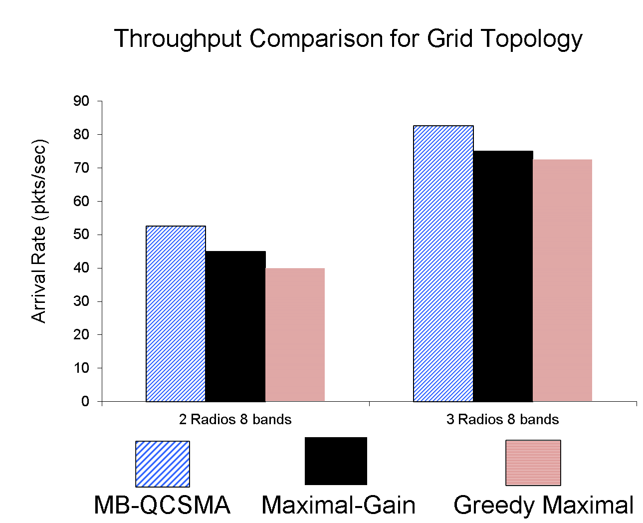
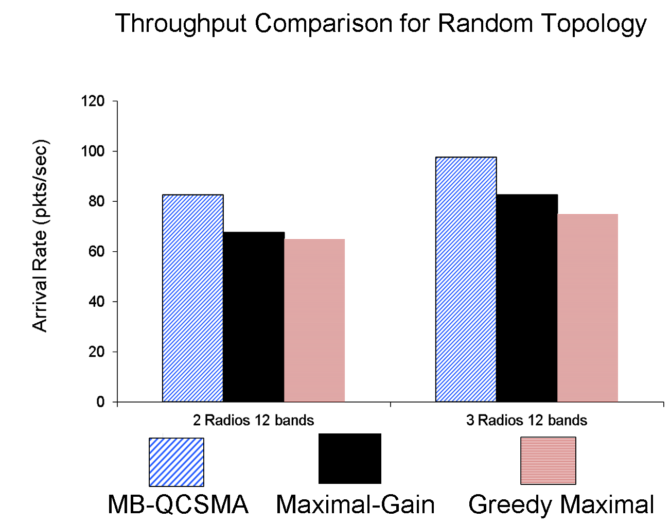
Figure 2: Throughput attained by Asyncronous Maximal Gain as compared to MB-QCSMA and MB-GMS. Note that, ignoring overheads, MB-CSMA achieves 100% throughput

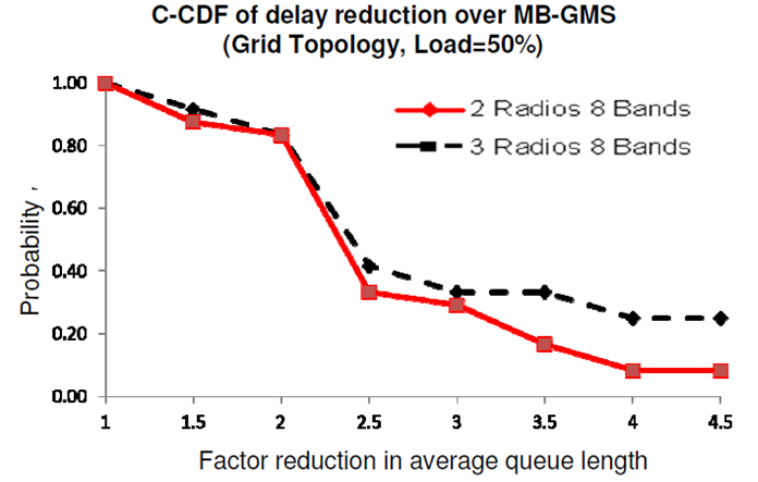
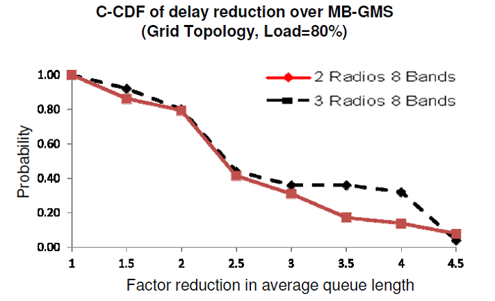
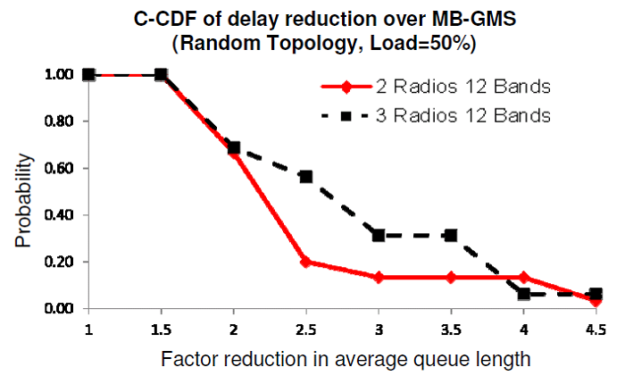
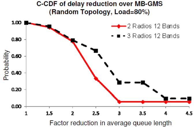
Figure 3: C-CDF of Delay Gains of Asynchronous Maximal Gain as Compared to MB-GMS.

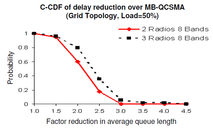
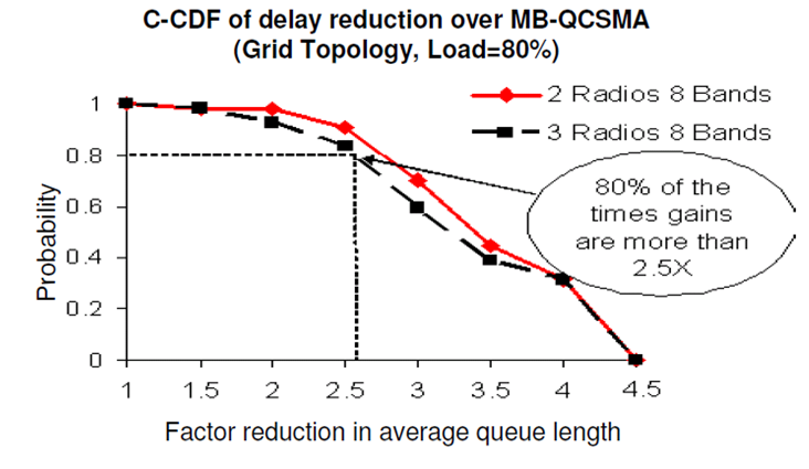
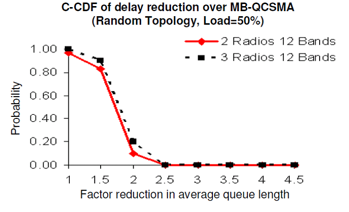
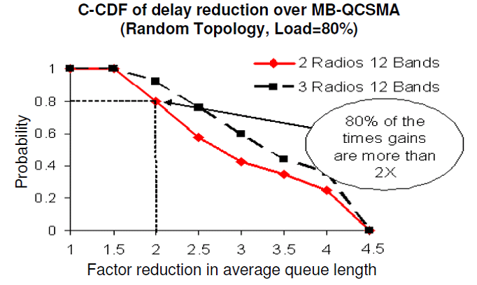
Figure 4: C-CDF of Delay Gains of Asynchronous Maximal Gain as Compared to MB-QCSMA.

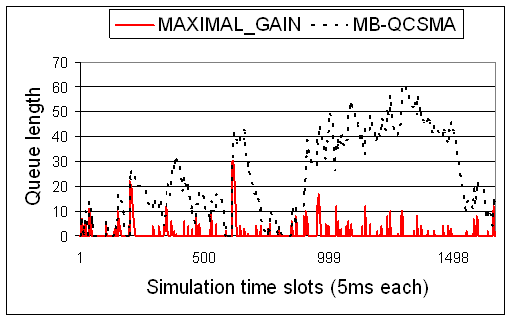
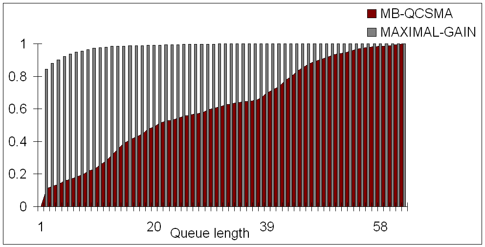
Figure 5: (a): Queue evolution of a typical bottleneck node over 10 seconds. (b): CDF of the queue length values of a bottleneck node over 10 seconds. Note that the probability of queue length being less than 25 is close to 50% with MB-QCSMA while it is close to 100% in MAXIMAL-GAIN.

Delay gains: We compare the network-wide average delay of MAXIMAL-GAIN with MB-GMS (Figure 3) and MB-QCSMA (Figure 4). We show the C-CDF of delay improvements (average queue length with MB-QCSMA / Average queue length with MAXIMAL-GAIN) with our asynchronous algorithm for a moderate load (50%) and high load (80%). to answer the question : how often are the delay gains significant? We show the results for 25 node grid deployment with 8 bands and 25 node random deployment with 12 bands. Compared to MB-QCSMA, as shown in Figure 4, under medium load conditions, the gains are $2\times$ ($1.75\times$) or more in 50% of the runs, and $1.75\times$ ($1.5\times$) or more in 80% of the runs for grid (random) topology. Also, compared to MB-GMS, as shown in Figure 3, under high-load conditions the gains are $2\times$ ($2.25\times$) or more in 50% of the runs, and $1.75\times$ ($2\times$) or more in 80% of the runs for grid (random) topology. Similar gains were observed with 12 (8) bands for grid (random) topologies.

To understand this network-level behaviour more clearly, we observe the behavior of queues at individual nodes in the network. Figures 5 and  5 plot the queue evolution of one of the congested nodes in the network over a period of 10 seconds. We clearly see that the MB-QCSMA algorithm allows the queue size to grow large before giving the link preferential treatment and draining it. On the other hand, the MAXIMAL-GAIN algorithm drains all queues more uniformly. In Figure 5, we plot the CDF of the queue sizes and we observe that, with MAXIMAL-GAIN, queue length is less than 10 for 97% of the time, whereas queue length is less than 10 in only 15% of the time with MB-QCSMA. We also observed similar trends in comparison to MB-GMS.

Our key takeaways are as follows:

• The delay gains are more significant (typically in the range $2\--4\times$) under heavy load.

• The gains are more prominent for regular topologies like grid, pointing towards the increased benefit of our MAC in scenarios of careful network deployment.

• Our algorithm not only shows gains in average queue-length or delay, but also ensures short queue-lengths on most times during network operation. Thus, our MAC allows the designer to use a small MAC-layer buffer.

Throughput loss: We increase the average arrival rates for flows in the network, till the queues at the nodes start exploding. We call the maximum average arrival rate that the network can support as the maximum stabilizable rate of the network under a given scheduling algorithm. As shown in Figure 2, the maximum stabilizable rate of MAXIMAL-GAIN algorithm is within 80-90% of the maximum stabilizable rate of Q-CSMA algorithm. Also, in most instances, the throughput attained by our algorithm is on par with or better than MB-GMS. Thus, we summarize that, the throughput loss of our delay oriented MAXIMAL-GAIN MAC is no more than $10\--20\%$.

Robustness: MAXIMAL-GAIN algorithm requires the leader to overhear all RTS/CTS communications in the group for correct operation. In practice, it is possible that the leader does not hear all RTS/CTS messages, due to collisions and losses and hence has some outdated information. To measure the robustness of our algorithm to such gaps in accuracy, we vary the probability with which the RTS/CTS messages are overheard by the leader and measure the resulting throughput and delay in the network. We did not observe any significant drop in either throughput or delay performance across several runs even when the probability of not hearing messages was increased to 50%. Thus, our algorithm is robust to somewhat outdated information.

VII Conclusion

In this paper we have shown that design of practical distributed algorithms for multi-band multi-radio networks are possible that achive low delays, almost achieve full throughput, and have low overhead and complexity.

Appendix A Proof of Theorem 1

We will start by proving Part 1 of Theorem 1. Then, we will show that the Part 2 of Theorem 1 follows from Part 1 along the lines of proof of delay bound in [18].

Proof of Part 1 of Theorem 1: The max-weight ($\mathsf{MW}$) schedule, defined by the schedule that maximizes the total weight (queue length times the link rate), in every time-slot stabilizes the network [33]. In [11], the result was generalized to show that, any schedule such that the total weight differs from the max-weight schedule at most by an additive constant also stabilizes the network. While [11] showed it for switch scheduling, the technique is very general and can be adapted to show the following generic result for our framework.

Lemma A.1 (Adapted from [11]).

Suppose a randomized algorithm has total weight $W(t)$ at time $t$ and let $W^{*}(t)$ be the weight of the $\mathsf{MW}$ schedule. If

$$\mathbb{E}\left[W^{*}(t)-kW(t)\right]<C\ ,$$ (5)

for some $C<\infty$ and $k<\infty$, then the algorithm stabilizes any arrival $\bf{\lambda}\in\frac{\Lambda}{k}$.

Thus, if we show that MAXIMAL-GAIN schedule satisfies (5) for $k=\mu$ as defined in Theorem 1, then Part 1 immediately follows. We will now argue that the condition given by (5) is satisfied by a scheduling algorithm, if the following inequality holds for some $\lvert\alpha\rvert<1$:

$$\mathbb{E}[W^{*}(t)-\mu W(t)]\leq\alpha\mathbb{E}[W^{*}(t)-\mu W_{-1}(t)]\ ,$$ (6)

where $W_{-1}(t)$ is the total weight at time $t$ of the schedule at time $t-1$ (denoted by $S_{t-1}$). In other words, if we activate at time $t$ the same set of links as the schedule at $t-1$, the total weight is denoted by $W_{-1}(t)$. We will now show (6)$\Rightarrow$(5).

First consider the case $0\leq\alpha<1$. We introduce some notations. Let $\delta_{1}$ be the upper bound on the expected total weight increase that is possible from one slot to the subsequent slot if the arrival rates are in the stable region. Similarly, let $\delta_{2}$ be the bound on maximum decrease in weight possible from one slot to the subsequent slot. Clearly, there exists $\delta_{1}<\infty$ because

$${\mathbb{E}}[W^{*}(t)\ |\ W^{*}(t-1)] \leq W^{*}(t-1)+\sum_{h\in{\mathcal{H}}}{\mathbb{E}}[A_{h}(t)]$$

$$=W^{*}(t-1)+\sum_{h}\lambda_{h}$$

$$\Rightarrow{\mathbb{E}}[W^{*}(t)] \leq{\mathbb{E}}[W^{*}(t-1)]+\sum_{h}\lambda_{h}$$

which follows from the fact that, from $t-1$ to $t$, each weight increases by at most the number of arrivals at $t$. Thus, we can choose $\delta_{1}=\sum_{h}\lambda_{h}$. Also, $\delta_{2}<\infty$ because the number of packets that can be served over a time slot is bounded. Now, using the facts that ${\mathbb{E}}[W^{*}(t)]\leq{\mathbb{E}}[W^{*}(t-1)]+\delta_{1}$ and $W_{-1}(t)\geq W(t-1)-\delta_{2}$ (because $W_{-1}(t)$ and $W(t-1)$ are the total weight of the same schedule but in successive time-slots), we have the following if (6) holds:

$$\mathbb{E}[W^{*}(t)-\mu W(t)]$$ (7)

$$\leq\alpha\mathbb{E}[W^{*}(t)-\mu W_{-1}(t)]$$

$$\leq\alpha(\mathbb{E}[W^{*}(t-1)]-\mu\mathbb{E}[W(t-1)])+\alpha(\delta_{1}+\mu\delta_{2})$$

$$\leq\alpha^{2}(\mathbb{E}[W^{*}(t-2)]-\mu\mathbb{E}[W(t-2)])+(\delta_{1}+\mu\delta_{2})(\alpha+\alpha^{2})$$

$$\leq\frac{\alpha}{1-\alpha}((\delta_{1}+\mu\delta_{2}))\ ,$$

where, we have assumed that the system was started at time $t=-\infty$ with $W^{*}=0$ and $W=0$.

The case when $-1<\alpha\leq 0$ follows by defining $\delta_{1}$ as the upper bound on the decrease of expected total weight that is possible from one slot to the subsequent slot, and by defining $\delta_{2}$ be the bound on maximum increase in weight possible from one slot to the subsequent slot. A similar calculation can then be performed.

Thus, we have argued that, (6) implies (5) with $k=\mu$ which in turn implies Part 1 of Theorem 1. The following Lemma asserts that Equation 6 holds from which the desired result follows.

Lemma A.2.

The Maximal-Gain algorithm satisfies

$$\mathbb{E}\left[W^{*}(t)-\mu W(t)\right]\leq\alpha\mathbb{E}\left[W^{*}(t)-\mu W_{-1}(t)\right]\ ,$$

where

$$\mu=\beta_{\max}(1+2(1+\kappa_{1}))\ ,\ \alpha=1-(\theta+{\textstyle{\frac{\theta}{2(1+\kappa_{1})}}})\ ,$$

and $\theta=1-(1-{\textstyle{\frac{1}{M}}})^{1+\kappa_{1}}$.

Remark 6.

Note that $\lvert\alpha\rvert<1$ because $0<\theta+{\theta}/{(2(1+\kappa_{1}))}<2$. This is true for any $M$ and $\kappa_{1}$.

Proof.

Let $S_{t}$ be the set of activated/scheduled links in time slot $t$ and let $S_{t}(f_{j})$ be the set of those links that operate over frequency band $f_{j}$. We will index by $k$ the groups formed by the grouping in MAXIMAL-GAIN scheduling. Let $L_{k}(j,t)\subseteq S_{t}(f_{j})$ be the set of all generalized links on band $f_{j}$ activated at time $t$ such that the node tail($l$) belongs to group $k$.

First, we lower bound $W(t)-W_{-1}(t)$. To do this, we consider two kinds of links: winner links that are egress from a node based on the outcome of Algorithm LOCAL-MAX described in Section IV-B, and every other links that were also active in the previous time slot but who lose their weight as new winner links get activated. Clearly, the winner nodes that become a part of the schedule deactivate some links in their interference neighborhood. Let $W^{+}(t)$ be the random variable denoting the total gain in weight of winner links at time $t$ compared to their total weight if $S_{t-1}$ was also used at time $t$; and let $W^{-}(t)$ the random variable denoting the loss in weight of deactivated links compared to their total weight if $S_{t-1}$ was also used at time $t$.

$$W(t)-W_{-1}(t)=W^{+}(t)-W^{-}(t)$$ (8)

In the following, we will first lower bound ${\mathbb{E}}[W^{+}(t)|S_{t},\mathbf{w}(t)]$ and then upper bound ${\mathbb{E}}[W^{-}(t)|S_{t},\mathbf{w}(t)]$. We will now introduce some notations. Recall that in the MAXIMAL-GAIN algorithm, each group leader selects a band at random and picks the links with the maximum gain to transmit. This link then does CSMA contention to transmit on the chosen band. It may well be that the chosen link is unable to transmit since some other link in an interfering group wins the contention on that band. Define the indicator variable $I_{k,j}$ as

$$I_{k,j}=\left\{\begin{array}[]{ll}1&\text{if group $k$ chooses band $f_{j}$ at random}\\ &\text{and winner captures channel}\\ &\\ 0&\text{else}\end{array}\right.$$

We also define

$$I^{\max}_{k,j}=\left\{\begin{array}[]{ll}1&\text{if group $k$ succeeds in computing}\\ &\text{ the max gain in the group}\\ &\\ 0&\text{else}\end{array}\right.$$

Now define $d_{l}(t)$ and $e_{l}(t)$ as the total weight decrease due to deactivation of other active links (that were active in $S_{t-1}$) at tail($l$) and head($l$), respectively. Now note that, for all possible sample paths, we can bound the random variable $W^{+}(t)$ as

$$W^{+}(t)\geq\sum_{k,j}I_{k,j}I^{\max}_{k,j}\max_{l\in L_{k}(j,t{{\color[rgb]{0,0,0}-1}})}(([w_{l}(t)r_{l}-d_{l}(t)])^{+})$$ (9)

because the term $\max_{l\in L_{k}({{\color[rgb]{0,0,0}f_{j},t-1}})}[w_{l}(t)r_{l}-d_{l}(t)]^{+}$ represents the maximum gain in group $k$ at time $t$ (see eqn. (1) in Step-4(2) of Algorithm I). We also have,

$$\max_{l\in L_{k}(j,t{{\color[rgb]{0,0,0}-1}})}[w_{l}(t)r_{l}-d_{l}(t)]^{+}$$

$$\geq \max_{l\in L_{k}(j,t{{\color[rgb]{0,0,0}-1}})\cap L^{*}(j,t)}[w_{l}(t)r_{l}-d_{l}(t)]^{+}$$

$$\geq \max_{l\in L_{k}(j,t{{\color[rgb]{0,0,0}-1}})\cap L^{*}(j)}[w_{l}(t)r_{l}]-\sum_{l\in L_{k}(j,t{{\color[rgb]{0,0,0}-1}})}d_{l}(t)$$

Here $L^{*}(j,t)$ is the set links of which are allocated band $j$ in the optimal allocation at time $t$. The first step follows from the fact constraining the allocation over the set $L_{k}(j,t)\cap L^{*}(j,t)$ will only decrease the value of the expression, and the second step follows from the fact that maximum of values of elements is less than the sum of their values. Note that we have,

$${{\color[rgb]{0,0,0}\max_{l\in L_{k}(j,t-1)\cap L^{*}(j,t)}[w_{l}(t)r_{l}]\geq\frac{1}{\beta_{\max}}\sum_{l\in L_{k}(j,t-1)\cap L^{*}({j},t)}{w_{l}(t)r_{l}}}},$$

where $\beta_{\max}$ is the interference degree of the network. This is because $\max$ is greater than the average and there can be at most $\beta_{\max}$ links active on a band in a group. We thus have

$$\max_{l\in L_{k}(j,t{{\color[rgb]{0,0,0}-1}})}[w_{l}(t)r_{l}-d_{l}(t)]^{+}$$

$$\geq\left(\sum_{l\in L_{k}(j,t{{\color[rgb]{0,0,0}-1}})\cap L^{*}(j,t)}\frac{{{\color[rgb]{0,0,0}w_{l}(t)r_{l}}}}{\beta_{\max}}-\sum_{l\in L_{k}(j,t{{\color[rgb]{0,0,0}-1}})}d_{l}(t)\right)^{+}$$ (10)

Substituting (10) in (9) followed by taking expectations in (9), we obtain

$${\mathbb{E}}\left[W^{+}(t)|S_{t-1},\mathbf{w}(t)\right]$$ (11)

$$\geq\sum_{k,j}{\textstyle{\frac{1}{2}}}p_{k,j}\left(\sum_{l\in L_{k}(j,t{{\color[rgb]{0,0,0}-1}})\cap L^{*}{{\color[rgb]{0,0,0}(j,t)}}}\frac{{{\color[rgb]{0,0,0}w_{l}(t){{\color[rgb]{0,0,0}r_{l}}}}}}{\beta_{\max}}-\sum_{l\in L_{k}(j,t)}d_{l}(t)\right)^{+}\ ,$$

where $\Pr\{I_{k,j}=1\}=p_{k,j}$ and we have also used the fact that $\Pr\{I^{\max}_{k,j}=1\}\geq 1/2$ (from Lemma IV.1). Denoting by $X_{k,j}$ the random variable for the number of winner links of other groups on band $j$ that interfere with group $k$’s winner at time $t$ (these links are also picked as winners by their respective leaders over the same band as $k$). Assuming that the contention resolution is perfect in the sense that (i) with probability one, at least one of the contending nodes grab channel access, and (ii) all contending nodes are equally likely to get channel access, we can now bound $p_{k,j}$ as follows:

$$p_{k,j}=\Pr(\text{leader chooses band $f_{j}$})$$

$$\ \ \times\Pr\left(\begin{array}[]{c}\text{winner link in group}\\ \text{wins contention}\end{array}\ |\ \text{band $f_{j}$ is chosen}\right)$$

$$=\frac{1}{M}{\mathbb{E}}\left[\frac{1}{1+X_{k,j}}\right]$$

Since the number of interfering links of winner link in a group is upper bounded by $\kappa_{1}$, $X_{k,j}$ can shown to be stochastically dominated from above by the distribution $\textsc{Bin}(\kappa_{1},1/M)$ (i.e., $\Pr(X_{k,j}\geq n)\leq\Pr(\textsc{Bin}(\kappa_{1},1/M)\geq n)\ \forall n\geq 0$). Thus it follows that,

$$p_{k,j} \geq\frac{1}{M}{\mathbb{E}}\left[\frac{1}{1+\textsc{Bin}(\kappa_{1},{\textstyle{\frac{1}{M}}})}\right]$$ (13)

$$=\frac{1}{M}\sum_{n=0}^{\kappa_{1}}{\textstyle{\frac{1}{1+n}}}{\kappa_{1}\choose n}\left({\textstyle{\frac{1}{M}}}\right)^{n}\left(1-{\textstyle{\frac{1}{M}}}\right)^{\kappa_{1}-n}={\textstyle{\frac{\theta}{1+\kappa_{1}}}}\ ,$$

where $\theta=1-(1-1/M)^{\kappa_{1}+1}$ and the last equality follows from standard computations with Binomial distribution. Substituting (13) into (11) we obtain the following.

$${\mathbb{E}}\left[W^{+}(t)|S_{t-1},{\mathbf{w}}(t)\right]$$

$$\geq\frac{\theta}{2(1+\kappa_{1})}\sum_{k,j}\left({{\color[rgb]{0,0,0}\sum_{l\in L_{k}(j,t)\cap L^{*}(j,t-1)}{\textstyle{\frac{w_{l}(t){r_{l}}}{\beta_{\max}}}}}}\right.$$

$$-\left.\sum_{l\in L_{k}(j,t{{\color[rgb]{0,0,0}-1}})}d_{l}(t)\right)\geq\frac{\theta}{2(1+\kappa_{1})}\left({\textstyle{\frac{W^{*}{{\color[rgb]{0,0,0}(t)}}}{\beta_{\max}}}}{{\color[rgb]{0,0,0}-}}W_{-1}(t)\right)$$ (14)

We will now derive an upper bound on $W^{-}(t)$. Note that,

$${{\mathbb{E}}}\left[W^{-}(t)\ |\ S_{t-1},\mathbf{w}(t)\right]$$

$$=\sum_{l\in S_{t-1}}w_{l}(t)r_{l}.\Pr\left(\begin{array}[]{c}l\ \text{is in the interference neighborhood}\\ \text{of a winner link}\end{array}\right)$$ (17)

$$\leq\sum_{l\in S_{t-1}}w_{l}(t)r_{l}(1-(1-{\textstyle{\frac{1}{M}}})^{1+\kappa_{1}})=\theta W_{-1}(t)$$ (18)

Substituting, (14) and (18) into (8), we finally get

$${\mathbb{E}}[W(t)-W_{-1}(t)]\geq W^{*}(t)\frac{\theta}{2\beta_{\max}(1+\kappa_{1})}-(\theta+{\textstyle{\frac{\theta}{2(1+\kappa_{1})}}})W_{-1}(t)$$ (19)

which upon further rearrangement of term yields

$$\mathbb{E}\left[W^{*}(t)-\mu W(t)\right]\leq\alpha\mathbb{E}\left[W^{*}(t)-\mu W_{-1}(t)\right]$$

where

$$\mu=\beta_{\max}(1+2(1+\kappa_{1}))\ ,\ \alpha=1-(\theta+{\textstyle{\frac{\theta}{2(1+\kappa_{1})}}})\ ,$$

where $\theta=1-(1-{\textstyle{\frac{1}{M}}})^{1+\kappa_{1}}$. ∎

As argued before, Lemma A.2 implies Lemma A.1 with $k=\mu$ which in turn implies Part 1 of Theorem 1.

Proof of Part 2 of Theorem 1: This part follows along the lines of the delay analysis in  [18] with some minor modifications. See [7] for a proof sketch. $\blacksquare$

References

- [1] http://www.omnetpp.org.
- [2] FCC’s national broadband plan available at http://www.broadband.gov.
- [3] Radio technology systems http://www.radiotechnologysystems.com/.
- [4] Propagation data and prediction methods for the planning of short-range outdoor radiocommunication systems and radio local area networks in the frequency range 300 MHz to 100 GHz. Recommendation ITU-R P.1411, 1999.
- [5] E. Angel. A survey of approximation results for local search algorithms. In Efficient approximation and online algorithms, LNCS 3484 (2006), pages 30-73.
- [6] P. Chaporkar, K. Kar, and S. Sarkar. Throughput guarantees through maximal scheduling in wireless networks. In 43rd Annual Allerton Conf on Communications, Control, and Computing, Sep 2005.
- [7] A. Chatterjee, S. Deb, K. Nagaraj, and V. Srinivasan. Low Delay MAC Scheduling for Frequency-agile Multi-radio Wireless Networks. Alcatel-Lucent Technical Report, 2012.
- [8] S. Deb, V. Srinivasan, and R. Maheswari. Dynamic Spectrum Access in DTV Whitespaces: Design Rules, Architecture and Algorithms. In ACM MobiCom, 2009.
- [9] M. Dyer and M. Jerrum. On counting independent sets in sparse graphs. In IEEE FOCS, 1998.
- [10] D. T. G. Cafaro, N. Correal and J. Orlando. A 100 mhz 2.5 ghz cmos transceiver in an experimental cognitive radio system. In Proceeding of the SDR 07, 2007.
- [11] P. Giaccone, B. Prabhakar, and D. Shah. Randomized scheduling algorithm for high aggregate bandwidth switches. IEEE Journal on Selected Area in Communications, 21(4):546–559, 2003.
- [12] S. Jagabathula and D. Shah. Optimal delay scheduling in networks with arbitrary constraints. In ACM SIGMETRICS, 2008.
- [13] L. Jiang, M. Leconte, R. Srikant, and J. Walrand. Fast Mixing of Parallel Glauber Dynamics and Low-Delay CSMA Scheduling. In INFOCOM, 2011.
- [14] L. Jiang and J. Walrand. A distributed CSMA algorithm for throughput and utility maximization in wireless networs. In 46th Allerton Conference on Communications, Control, and Computing, 2008.
- [15] K. M. Jung and D. Shah. Low delay scheduling in wireless networks. In Proceedings of IEEE ISIT, 2007.
- [16] M. Kodialam and T. Nandagopal. Characterizing the capacity region in multi-radio, multi-channel wireless mesh networks. In ACM Mobicom 2005.
- [17] P. Kyasunur, J. Padhye, and P. Bahl. On the efficacy of separating control and data into different frequency bands. In IEEE Broadnets, 2005.
- [18] L. B. Le, K. Jagannathan, and E. Modiano. Delay analysis of maximum weight scheduling in wireless ad hoc networks. In CISS, 2009.
- [19] X. Lin and N. Shroff. The impact of imperfect scheduling on cross layer rate control in wireless networks. In IEEE Infocom, 2005.
- [20] X. Lin, N. B. Shroff, and R. Srikant. A tutorial on cross-layer optimization in wireless networks. IEEE Journal on Selected Areas in Communications, 24(8):1452–1463, 2006.
- [21] S. Merlin, N. Vaidya, and M. Zorzi. Resource allocation in multi-radio multi-channel multi-hop wireless netwoks. In IEEE INFOCOM, 2008.
- [22] M. Neely. Delay Analysis for Max Weight Opportunistic Scheduling in Wireless Systems. IEEE Transactions of Automatic Control, 2009.
- [23] M. J. Neely. Delay analysis for maximal scheduling in wireless networks with bursty traffic. In IEEE Infocom, 2008.
- [24] J. Ni, B. Tan, and R. Srikant. Q-csma:quelength based csma/ca algortithms for achieving maximum throughput and low delay in wireless networks. In IEEE Infocom Mini-Conference, 2010.
- [25] S. Parthasarathy and R. Gandhi. Distributed algorithms for coloring and domination in wireless ad hoc networks. In FSTTCS, 2004.
- [26] S. Rajagopalan, D. Shah, and J. Shin. Network Adiabatic Theorem: An Efficient Randomized Protocol for Contention Resolution. In ACM SIGMETRICS, 2009.
- [27] T. S. Rappaport. Wireless Communications, Principles and Practice. Prentice Hall, 2002.
- [28] S. Sarkar and K. Kar. Achieving 2/3 throughput approximation with sequential maximal scheduling under primary interference constraints. In 44th Annual Allerton Conference on Communication, Control and Computing, Allerton, Monticello, Illinois, September 2006.
- [29] D. Shah and J. Shin. Delay optimal queue-based CSMA. In ACM SIGMETRICS, 2010.
- [30] D. Shah, D. N. C. Tse, and J. Tsisiklis. Hardness of low delay network scheduling. IEEE Transactions on Information Theory, pages 7810-7817, 2011.
- [31] G. Sharma, R. R. Mazumdar, and N. B. Shroff. On the complexity of scheduling in wireless networks. In ACM Mobicom, 2006.
- [32] L. Tassiulas. Linear complexity algorithms for maximum throughput in radio networks and input queued switches. In Infocom, 1998.
- [33] L. Tassiulas and A. Ephremides. Stability properties of constrained queueing systems and scheduling policies for maximum throughput in multihop radio networks. IEEE Transactions on Automatic Control, 37(12), 1992.
- [34] W. C. X. C. Znati and T. X. L. Z. Lu. The complexity of channel scheduling in multi-radio multi-channel wireless networks. In IEEE Infocom, 2009.