Eigenvalue statistics of reduced density matrix during driving and relaxation

Abstract

We study a subsystem of an isolated one-dimensional correlated metal when it is driven by a steady electric field or when it relaxes after driving. We obtain numerically exact reduced density matrix $\rho$ for subsystems which are sufficiently large to give significant eigenvalue statistics and spectra of $\log(\rho)$. We show that both for generic as well as for the integrable model the statistics follows the universality of Gaussian unitary and orthogonal ensembles for driven and equilibrium systems, respectively. Moreover, the spectra of modestly driven subsystems are well described by the Gibbs thermal distribution with the entropy determined by the time-dependent energy only.

Introduction.— Spectral universality is one of the key features of highly excited complex systems. It has been demonstrated and observed in a diverse range of phenomenologies, ranging from acoustics Ellegaard et al. (1995), microwave resonators Stöckmann and Stein (1990); *stoeckmann1, quantum dots Marcus et al. (1992), to many-particle systems, such as complex nuclei Haq et al. (1982) and strongly correlated models of condensed matter Poilblanc et al. (1993). Universality is quantitatively characterized by the applicability of a parameter free random matrix theory (RMT) Mehta (2004), where the Hermitian operator in question, usually the Hamiltonian, is described by an ensemble of Gaussian random matrices, where the only constraint, whether matrices are real symmetric, or complex hermitian, is imposed by the existence, or non-existence of a (generalized) time-reversal symmetry. Random matrix distribution of energy levels is also widely used as a clean indicator of complexity, or non-integrability, of a physical model, and is the most abstract definition of a quantum chaotic behavior Haake (2001).

In this Letter we propose RMT analysis of a completely different concept in quantum statistical physics, namely of spectra of reduced density matrix (RDM) $\rho$ of equilibrium and non-equilibrium states. We consider RDM of strongly correlated quantum systems. In particular we study the one-dimensional (1D) model of interacting spinless fermions (equivalent to a Heisenberg–type spin chain) for a variety of simple pure states of the entire system: the so-called microcanonical (MC) states (approximate eigenstates), the time-evolving states after a quench of magnetic flux, or during inductive driving with a linearly increasing magnetic flux. We show that, quite remarkably, the statistics of eigenvalues of RDM of large subsystems is typically described by RMT. For equilibrium thermal states, we find agreement with Gaussian orthogonal ensemble (GOE), whereas for non-equilibrium, driven states, with currents, we find agreement with Gaussian unitary ensemble (GUE). We note in particular, that spectra of RDM of large subsystems typically follow RMT even if the entire system is completely integrable.

Furthermore, the RDM can serve as a stringent test of thermal properties of nonequilibrium states and their thermalization. Our results show that for modestly driven systems the entropy density $s$ of the subsystem develops in time according to the quasi-equilibrium scenario, i.e. $s$ depends only on the instantaneous energy density $\varepsilon$. In agreement with the latter is the observation for driven integrable and non–integrable chains that the eigenvalue spectra are consistent with the canonical Gibbsian form $\rho\propto\exp(-H_{\rm eff}/T)$ with well defined effective temperature $T$ and $H_{\rm eff}$ being a $T-$independent effective Hamiltonian of the subsystem.

Model and method.— We study the 1D model of interacting spinless fermions on a chain of even number of sites $L$ with periodic boundary conditions. We investigate how the system responds to an external electric field as introduced in the time-dependent model by the varying magnetic flux $\phi(t)$,

$$H(t) = -t_{0}\sum_{j}\left\{{\mathrm{e}}^{i\phi(t)/L}\;c^{\dagger}_{j+1}c_{j}+{\mathrm{h}.c.}\right\}$$ (1)

$$+V\sum_{j}\hat{n}_{j}\hat{n}_{j+1}+W\sum_{j}\hat{n}_{j}\hat{n}_{j+2},$$

where $\hat{n}_{j}=c^{\dagger}_{j}c_{j}$, $t_{0}$ is the hopping integral, $V$ and $W$ are the repulsive potentials between fermions on the nearest-neighbor and the next-nearest-neighbor sites. Furtheron we use units in which $\hbar=k_{B}=t_{0}=1$. The main idea behind introducing $W$ is to break integrability of the pure $t_{0}-V$ model. One expects generic properties for the non–integrable case with $W\neq 0$, whereas the integrable system ($W=0$) shows anomalous relaxation Rigol et al. (2007); Kollar et al. (2011); Cassidy et al. (2011); Steinigeweg et al. (2012) and transport characteristics Zotos and Prelovšek (1996); Mierzejewski and Prelovšek (2010); Mierzejewski et al. (2011); Prosen (2011); Žnidarič (2011); Sirker et al. (2009); Steinigeweg and Brenig (2011). If not stated otherwise, the numerical results for integrable and non–integrable cases will refer to $V=1$, $W=0$ and $V=1.4$, $W=1$ systems, respectively, at half-filling with $M=L/2$ fermions on $L=26$ sites. These parameters correspond to the metallic regime.

In the numerical procedure using the microcanonical (MC) Lanczos method Long et al. (2003) we generate initial states $|\Psi(0)\rangle$ for the target energy $E_{0}=\langle\Psi(0)|H(0)|\Psi(0)\rangle$ and the energy uncertainty $\delta^{2}E_{0}=\langle\Psi(0)|[H(0)-E_{0}]^{2}|\Psi(0)\rangle$. Typically, we consider large $E_{0}$ (corresponding to high $T$, i.e. $\beta\equiv 1/T<0.5$) with $L=26$ and $\delta\simeq 0.01$. To simulate the MC ensemble, the energy window is small on a macroscopic scale ($\delta E_{0}/E_{0}\ll 1$) but still contains a large number of levels Goldstein et al. (2006). The time evolution of $|\Psi(0)\rangle\rightarrow|\Psi(t)\rangle$ is calculated by Lanczos propagation method Park and Light (1986) applied to small time intervals $(t,t+\delta t)$.

Since the entire chain is isolated from the surroundings it remains in a pure state $|\Psi(t)\rangle\langle\Psi(t)|$. In this Letter we focus on the reduced dynamics of its subsystem containing $N$ subsequent lattice sites. The RDM of the subsystem is then $\rho=\mathrm{Tr}_{L-N}|\Psi(t)\rangle\langle\Psi(t)|$ where the trace is taken over the remaining $L-N$ sites. RDM is block–diagonal with respect to number of particles in the subsystem $n=\sum_{i=1}^{N}n_{i}={0,...,N}$. As the approach is numerically accurate the reduced dynamics is exact as well. At the same time, the approach allows for subsystems which are sufficiently large to give meaningful level statistics as well as spectral and other properties of $\rho$. With respect to time-dependent response we study two kinds of systems: a) driven by a steady electric field $F=-\partial_{t}\phi(t)/L=\mathrm{const}$, and b) relaxing but not necessarily thermalizing after a sudden quench of the flux (field pulse): $\phi(t)=\theta(t)\delta\phi$.

Eigenvalues statistics of RDM— We start with the presentation of results on the eigenvalue statistics of $\log(\rho)$. For the quasi–thermal states $\rho\propto\exp(-\beta H_{\rm eff})$ the statistics of eigenvalues of $\log(\rho)$ should be the same as the level statistics of the effective Hamiltonian. Since we can reach using MC Lanczos method (at half-filling) systems with $L=26$ the eigenvalue statistics is determined for the largest accessible subsystems of $N=12$ sites and $n=6$ fermions (containing 924 levels). We note that even though the number $n$ of fermions within the subsystem is not conserved, RDM is block-diagonal with respect to states with fixed $n$, hence $[H_{\rm eff},n]=0$. The spectrum $\left\{\lambda_{i}\right\}$ of $\log(\rho)$ is unfolded by a linear interpolation of the integrated density ${\cal N}(\omega)=\sum_{i}\theta(\omega-\lambda_{i})$ in intervals containing $40$ subsequent eigenvalues. This procedure leads to a smoothened integrated density ${\cal N}_{\mathrm{s}m}(\omega)$. The unfolded spectrum consists of $\bar{\lambda}_{i}={\cal N}_{\mathrm{s}m}(\lambda_{i})$ where we analyze only $~{}2/3$ of eigenvalues from middle of this spectrum (see Bruus and Angl‘es d’Auriac (1997) for more details on unfolding). We study in the following two standard quantities characterizing the level statistics: a) the nearest-level-spacing distribution $p(x)$ and the eigenvalue number variance $\Sigma^{2}(\delta)$ defined as the variance of the number of unfolded eigenvalues in the interval of length $\delta$. $p(x)$ and $\Sigma^{2}(\delta)$ characterize local correlation properties of the spectrum and long-range level correlations, respectively. The numerical results for $\log(\rho)$ can be compared with the results of the RMT for the GOE or GUE ensembles Brody et al. (1981); Guhr et al. (1998),

$$p_{\mathrm{GOE}}(x) \simeq \frac{\pi x}{2}\exp(-\pi x^{2}/4),$$ (2)

$$\Sigma^{2}_{\mathrm{GOE}}(\delta) \simeq \frac{2}{\pi^{2}}\left(\log(2\pi\delta)+\gamma+1-\frac{\pi^{2}}{8}\right),$$ (3)

$$p_{\mathrm{GUE}}(x) \simeq \frac{32x^{2}}{\pi^{2}}\exp(-4x^{2}/\pi),$$ (4)

$$\Sigma^{2}_{\mathrm{GUE}}(\delta) \simeq \frac{1}{\pi^{2}}\left(\log(2\pi\delta)+\gamma+1\right),$$ (5)

where $\gamma\simeq 0.577$ is the Euler constant. Note that Hamiltonians of many-body integrable systems have the Poisson distribution with $p_{\mathrm{P}}(x)=\exp(-x)$ and $\Sigma^{2}_{\mathrm{P}}(\delta)=\delta$, while generic non-integrable systems with the time–reversal symmetry are expected to follow the GOE statistics. Only cases breaking the time-reversal symmetry should result in the GUE statistics.

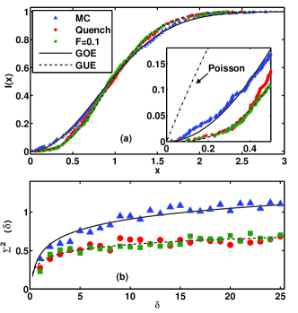
Figure 1: (Color online) Eigenvalue statistics of $\log(\rho)$ of the integrable system: in the equilibrium MC state, in the quasi-equilibrium evolution during driving ($F=0.1$), and in the non–thermal steady state after quenching the flux (Quench). Panel (a) shows the integrated spacing distribution $I(x)$ with the inset zoom in the low–gap regime, and b) the level number variance $\Sigma_{2}(\delta)$. Lines show results from the RMT.

We first analyze the spectrum of $\log(\rho)$ for the initial MC state in a generic non–integrable system and find that both $p(x)$ and $\Sigma^{2}(\delta)$ accurately reproduce the results for GOE (not shown). It is expected since in this case without a flux the time-reversal symmetry is preserved and $\rho$ can be chosen as a real symmetric matrix. In Fig. 1 we present numerical data for the integrable system together with the prediction of the RMT. The upper panel shows integrated spacing distribution $I(x)=\int^{x}_{0}\mathrm{d}yp(y)$, whereas $\Sigma^{2}(\delta)$ is shown in the lower panel. Surprisingly, the eigenvalue statistics of the RDM of a subsystem turns out to be independent of the integrability of the total system.

On the other hand, under a constant (but modest) field $F>0$ Mierzejewski and Prelovšek (2010); Mierzejewski et al. (2011) or after a sudden flux quench Rigol and Srednicki (2012) we find that the statistics turn into GUE. This is the case for the non–integrable systems as well as for the integrable one, as clearly confirmed in Fig. 1. The GUE statistics at $F>0$ is consistent with the time–symmetry breaking by a finite current within the subsystem. In the case of quenching the decay of the current is not complete, at least not within an integrable system where the absence of the current relaxation is a hallmark of a finite charge stiffness Zotos and Prelovšek (1996). We have determined the eigenvalue statistics also for the far-from-equilibrium driven states, shortly after the electric field has been switched on (not shown). The eigenvalues of $\log(\rho)$ are very similar to those presented in Fig. 1 for the GUE level case, indicating that the RMT statistics of $\log(\rho)$ is very robust.

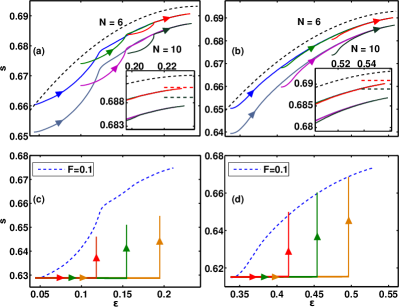
Figure 2: (Color online) Instantaneous entropy density $s(t)$ vs. energy density $\varepsilon(t)$ for integrable (a,c) and non–integrable (b,d) metals. Panels (a,b) show results for systems driven by field $F=0.1$ and $N=6,10$ subsystems. Dashed curves represent high–$T$ analytic results, Eq. (9) for $L\rightarrow\infty$. In the insets the high-$\varepsilon$ regime is magnified and $1/L$ corrections to $s_{\infty}$ are included and marked as horizontal lines. Panels (c,d) show relaxation after flux quenching for $N=12$ subsystem. Here, dashed curves show quasi-equilibrium results for the same systems driven with $F=0.1$. Arrows mark the direction of the processes.

Subsystem entropy density- While the von Neumann entropy of the total system is at all times zero for the pure state $|\Psi(t)\rangle\langle\Psi(t)|$, the (entanglement) entropy of the subsystem $S=-\mathrm{Tr}_{N}(\rho\log\rho)$ is clearly not. As a strong indication of the thermal (or quasi-equilibrium) states we can use the relation of the subsystem entropy density $s=S/N$ and the energy density $\varepsilon=\langle H(t)\rangle/L$ of the total system (being the same for the subsystem). Hence, we present in Fig. 2 the time-evolution of $s(t)$ plotted versus $\varepsilon(t)$ for two systems: driven by a constant electric field $F=0.1$ (panels a,b) and after a sudden flux quench (panels c,d). Results in the right and left panels are for the non–integrable and integrable cases, respectively. Note first that $s(t)$ only weakly depends on $N$ confirming its macroscopic relevance Santos et al. (2012). This is in contrast with a specific case of the ground state where we have found $s(0)\propto N^{-1}$ in agreement with the so called area laws for the entanglement entropy Eisert et al. (2010).

Since we are studying the high-$T$ regime it is instructive to recall the equilibrium result following from straightforward high temperature expansion (HTE),

$$\varepsilon = \varepsilon_{\infty}-\beta\sigma^{2}_{\infty},$$ (6)

$$\varepsilon_{\infty} \simeq \frac{V+W}{4}(1-\frac{1}{L}),$$ (7)

$$\sigma^{2}_{\infty} \simeq \frac{t^{2}}{2}+\frac{V^{2}+W^{2}}{16}+\frac{t^{2}}{2L}-\frac{VW}{4L}$$ (8)

where $\varepsilon_{\infty},\sigma_{\infty}$ refer to $T=\infty$ and $1/L$ corrections emerge due to a restriction of strictly $M=L/2$ fermions in the whole system. Integrating the equilibrium relation $\beta=\partial s/\partial\varepsilon$ one gets for the equilibrium entropy density

$$s(\varepsilon) = s_{\infty}-\frac{(\varepsilon_{\infty}-\varepsilon)^{2}}{2\sigma^{2}_{\infty}}$$ (9)

$$s_{\infty} \simeq \log(2)-\frac{N-1}{4L^{2}}-\frac{N^{2}-1}{6L^{3}},$$ (10)

where again leading $1/L$ corrections in $s_{\infty}<\log(2)$ arise due to fixing $M=L/2$. Insets in Figs. 2a,b show that our numerical results are very close to this simple estimate for $s_{\infty}$.

The relation (9) allows specifying regimes which are clearly nonequilibrium or steady but non–thermal. The former case occurs, e.g., just after turning on the electric field when $s=s(\varepsilon)$ is convex (see Figs. 2a and 2b) contrary to concave dependence, which according to Eq. (9) should characterize the quasi–equilibrium evolution. More interesting is the observation in Fig. 2c that the stationary non–thermal state emerges when integrable system relaxes after a sudden quench Rigol et al. (2007); Kollar et al. (2011) but $s(t)$ remains evidently smaller than expected for a thermal relation, Eq. (9).

Results shown in Fig. 2 may also suggest regimes, when the system even out of equilibrium reaches a quasi–thermal state. In this case $s(\varepsilon)$ should become independent of the initial state and close to the prediction of HTE. This indeed happens for integrable or non–integrable systems driven long enough by a moderate steady $F$ (note that $F$ breaks integrability of an integrable system) or when non–integrable system relaxes after the flux quench (see Fig. 2d).

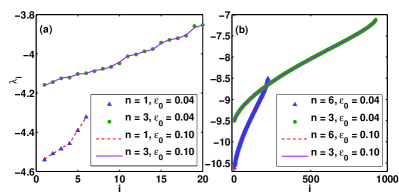
Figure 3: (Color online) Spectra of $\log[\rho(t)]$ for the integrable system driven by field $F=0.1$ determined at time $t$ such that $\varepsilon(t)=0.21$ but different initial energy densities $\varepsilon_{0}=0.04,0.1$ and different particle subsectors $n$. Panels (a) and (b) shows results for subsystems with $N=6$ and $N=12$ sites, respectively.

Thermal states- More stringent test for a thermal state is the requirement that the RDM obeys the canonical distribution $\rho\propto\exp[-\beta H_{\rm eff}(\phi)]$ whereby $H_{\rm eff}$ plays the role of an effective subsystem Hamiltonian. The effective inverse temperature $\beta$ can be also simply obtained from Eq. (6). The main open problem concerns the meaning of $H_{\rm eff}(\phi)$ when the subsystem is strongly coupled to its surroundings or is subject to external driving. However, we avoid this problem by testing the thermalization hypothesis without specifying the explicit form of $H_{\rm eff}(\phi)$.

In order to verify that the quasi–thermal state is determined solely by the energy density, we have determined the reduced dynamics of two identical subsystems (labelled by subscripts 1 and 2) driven by the same field $F=0.1$ but starting from different initial energies. We compare $\rho_{1}(t_{1})$ and $\rho_{2}(t_{2})$ for such times $t_{1}$ and $t_{2}$ that both systems have the same instantaneous energies (temperatures) $E(t_{1})=E(t_{2})$. Then, one expects $\log[\rho_{1}(t_{1})]=-\beta H_{\rm eff}[\phi(t_{1})]+\mathrm{const}$ and $\log[\rho_{2}(t_{2})]=-\beta H_{\rm eff}[\phi(t_{2})]+\mathrm{const}$. In other words, for the quasi thermal state operators $\log[\rho_{1}(t_{1})]$ and $\log[\rho_{2}(t_{2})]$ should give Hamiltonians of the same system but at least subject to different fluxes. Such Hamiltonians may have different eigenfunctions but the energy spectrum should be the same (up to eigenvalue fluctuations discussed above). Fig. 3 shows results testing the above hypothesis for two different subsystems $N=6,12$ and two sectors $n$, respectively. It is quite evident that the spectra are independent of the initial MC energy density $\epsilon_{0}$, at least for the states for which the results on entropy already suggested possible thermalization.

Fig. 4a finally shows spectra of $\log[\rho(t)]$ for driven integrable system (only the largest sector with $n=3$ is presented). Various curves are obtained for various times of driving, when the system has different instantaneous energies $\varepsilon(t)$. Together with Eq. (6) $\varepsilon(t)$ is used to determine the effective $\beta(t)$. For a quasi–thermal evolution the spectra of $\log[\rho(t)]/\beta(t)=-H_{\rm eff}[\phi(t)]+\mathrm{const}$ should be the same up to a constant value. As shown in Fig. 4b, even the driven integrable system perfectly fulfills this requirement. The thermalization of non–integrable systems is commonly expected (apart from a few more specific cases Manmana et al. (2007); Gogolin et al. (2011)), and our results (not shown) confirm that in general.

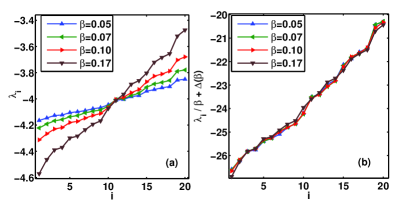
Figure 4: (Color online) Spectra of $\log[\rho]$ for the integrable system ($N=6,n=3$) driven by $F=0.1$ determined for $t$ corresponding to different $\beta(t)$ obtained from HTE. Panels (a) and (b) show eigenvalues of $\log[\rho]$ and normalized (and shifted) $\log[\rho]/\beta$, respectively.

Discussion.— Our study shows that the RDM $\rho$ of a subsystem within the isolated system of interacting fermions can be a useful tool to investigate properties of a nonequilibrium system. Our results on the RDM eigenvalue statistics within a 1D model of interacting spinless fermions reveal a universal conclusion, that subsystem of an equilibrium MC state obeys the GOE eigenvalue statistics, independent of integrability or non–integrability of the whole system (note that an integrable system as a whole obeys the Poisson statistics for the total energy eigenvalues). Moreover, subsystems of the driven system and systems quenched with a field pulse follow the GUE universality, although the model by itself does not break the time–reversal symmetry.

Further, the spectrum of $\log(\rho)$ contains information useful for identifying the quasi–thermal, steady non–thermal and the non–equilibrium regimes. For the case of quasi–thermal states, which are realized also for finite but modest driving, we have demonstrated that the effective inverse temperature $\beta$ as the only relevant parameter determines the spectra of eigenvalues of $\log(\rho)$. On one hand, this result sets straightforward limits on the relaxation of integrable systems. But possibly more importantly, it introduces a nontrivial concept of subsystem’s effective Hamiltonian $H_{\rm eff}$. The physical content and the usefulness of the latter, also its relation to the original full $H$ has still to be explored. In any case it gives a novel approach to investigations of non–equilibrium properties of isolated interacting systems, in particular in relation to their thermal and transport response.