On the effects of the evolution of microbial mats and land plants on the Earth as a planet. Photometric and spectroscopic light curves of paleo-Earths

Abstract

Understanding the spectral and photometric variability of the Earth and the rest of the solar system planets has become of the utmost importance for the future characterization of rocky exoplanets. As this is not only interesting at present times but also along the planetary evolution, we studied the effect that the evolution of microbial mats and plants over land has had on the way our planet looks from afar. As life evolved, continental surfaces changed gradually and non-uniformly from deserts through microbial mats to land plants, modifying the reflective properties of the ground and most probably the distribution of moisture and cloudiness. Here, we used a radiative transfer model of the Earth, together with geological paleo-records of the continental distribution and a reconstructed cloud distribution, to simulate the visible and near-IR radiation reflected by our planet as a function of Earth’s rotation. We found that the evolution from deserts to microbial mats and to land plants produces detectable changes in the globally averaged Earth’s reflectance. The variability of each surface type is located in different bands and can induce reflectance changes of up to 40% in period of hours. We conclude that using photometric observations of an Earth-like planet at different photometric bands, it would be possible to discriminate between different surface types. While recent literature propose the red edge feature of vegetation near 0.7 $\mu$$m$ as a signature for land plants, observations in near-IR bands can be equally or even better suited for this purpose.

1 INTRODUCTION

In the last decades, more than 850 exoplanets have been detected outside the solar system, while thousands of potential planet candidates from the Kepler mission are waiting for confirmation. Even though most of the discovered exoplanets are gas giants, as the larger planets are easier to detect than the smaller rocky ones, evolving observational capabilities have already allowed us to discover tens of planets in the super-Earth mass range (e.g. Udry et al. 2007; Charbonneau et al. 2009; Pepe et al. 2011; Borucki et al. 2012), some of them probably lying within the habitable zone of their stars (Borucki et al. 2012). Moreover, some Earth-sized, and even smaller, exoplanets have already been reported in the literature (Fressin et al. 2012; Muirhead et al. 2012). Indeed, early statistics indicate that about 62% of the Milky Way stars may host a super-Earth (Cassan et al. 2012). Thus, one can confidently expect that true Earth analogues will be discovered in large numbers in the near future.

To be prepared for the characterization of future exoearth detections, the exploration of our own solar system and its planets is essential. This will allow us to test our theories and models, enabling more accurate determinations, and characterization of the exoplanets’ atmospheres and surfaces. In particular, observation of the solar system rocky planets, including Earth, will be key for the search for life elsewhere.

Over the last years, a variety of studies, both observational and theoretical, to determine how the Earth would look like to an extrasolar observer have been carried out. One of the observational approaches has been to observe the Earthshine, i.e., the sunlight reflected by Earth via the dark side of the moon. The visible spectrum of the Earthshine has been studied by several authors (Goode et al. 2001; Woolf et al. 2002; Qiu et al. 2003; Pallé et al. 2003, 2004), while more recent studies have extended these observations to the near-infrared (Turnbull et al. 2006) and to the near-UV (Hamdani et al. 2006).

Several authors have also attempted to measure the characteristics of the reflected spectrum and the enhancement of Earth’s reflectance at 700 nm due to the presence of vegetation, known as red-edge, directly (Arnold et al. 2002; Woolf et al. 2002; Seager et al. 2005; Montañés-Rodríguez et al. 2006; Hamdani et al. 2006), and also by using simulations (Tinetti et al. 2006a, b; Montañés-Rodríguez et al. 2006). The red-edge has been proposed as a possible biomarker in Earth-like planets (Tinetti et al. 2006c; Kiang et al. 2007a, b). Furthermore, Pallé et al. (2008) determined that the light scattered by the Earth as a function of time contains sufficient information, even with the presence of clouds, to accurately measure Earth’s rotation period. More recently, Sterzik et al. (2012) have also studied the use of the linear polarization content of the Earthshine to detect biosignatures, and were able to determine the fraction of clouds, oceans, and even vegetation.

Another approach has been to analyze Earth’s observations from remote-sensing platforms (e.g., Cowan et al. 2009, 2011; Robinson et al. 2011). These kinds of observations have also allowed the possibility to reconstruct the continental distribution of our own planet from scattered light curves. Cowan et al. (2009) performed principal components analysis in order to reconstruct surface features from the EPOXI data. Kawahara & Fujii (2010, 2011) and Fujii & Kawahara (2012) proposed an inversion technique which enables to sketch a two-dimensional albedo map from annual variations of the disk-averaged scattered light. In addition, Oakley & Cash (2009) attempted to reproduce a longitudinal map of the Earth from simulated photometric data by using the difference in reflectivity between land and oceans. Other authors have also studied what the color of an extreme Earth-like planet might be by utilizing filter photometry (Hegde & Kaltenegger 2013), while others have studied the disk-averaged spectra of cryptic photosynthesis worlds (Cockell et al. 2009).

However, it is unlikely that, even if we were to find an Earth-twin, planet will be at an evolutionary stage similar to the Earth is today. On the contrary, extrasolar planets are expected to exhibit a wide range of ages and evolutionary stages. Because of this, it is of interest not only to use our own planet, as it is today, as an exemplar case, but also at different epochs (Kaltenegger et al. 2007).

The development of advanced plants is believed to have taken place on Earth during the Late Ordovician, about 450 Ma ago, albeit fungi, algae, and lichens may have greened many land areas before then (Gray et al. 1985). Microbial mats are multilayered sheets of microorganisms generally composed of both Prokaryotes and Eukaryotes, being able to reach a thickness of a few centimeters. The time when microbial mats appeared on the Earth surface is still not clear, but prior to the evolution of algae and land plants on early Earth, photosynthetic microbial mats probably were among the major forms of life on our planet. Microbial mats are found in the fossil record as early as 3.5 billion years ago. Later, when advanced plants and animals evolved, extensive microbial mats became rarer, but they are still presented in our planet in many ecosystems (Seckbach & Oren 2010). Even today, they still persist in special environments such as thermal springs, high salinity environments, and sulfur springs.

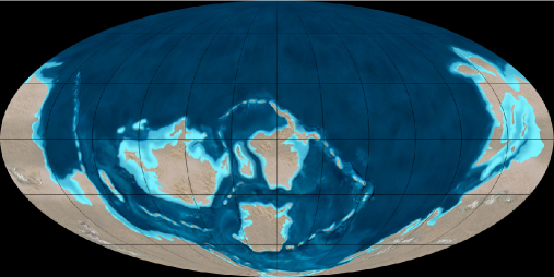
Figure 1: Geologic map of the Earth during the Late Cambrian (500 Ma ago). In our simulations the meridian line crossing the image center has been taken as longitude 0. Image credit: Ron Blakey.

In this paper, we aimed to discern the effect that the evolution of life over land might have had on the way our planet would look like to a remote extraterrestrial observer. To this end, we have simulated both visible and near-IR disk-integrated spectra of our planet, considering as scenario of such simulations the Earth during the Late Cambrian (Figure 1), the period during which the development of the first plants is believed to have taken place. Thus, it is clear that as life evolved over land, Earth’s continental masses must have changed gradually going through different states that go from deserts, to microbial mats, to evolved plants.

2 MODEL DESCRIPTION

With the aim of deriving disk-averaged spectra of the Earth 500 Ma ago, at any viewing and illumination geometry, and for several surface types covering the continental crust, we have generated a database of one-dimensional synthetic radiance of the Earth, i.e., we have calculated synthetic spectra for a variety of surface and cloud types, and for several viewing and illumination angles. To do that, we have used a line-by-line radiative transfer algorithm, based on the DISORT (Discrete Ordinates Radiative Transfer Program for a Multi-Layered Plane-Parallel Medium) code (Stammnes et al. 1988).

Our radiative transfer model (RTM) uses profiles of temperature and atmospheric composition, spectral albedos of each surface type, and cloudiness information as input data for the calculations (see subsequent subsections for a detailed description of inputs). The code considers Earth’s atmosphere as plane-parallel, and its radiative properties are prescribed on a grid of contiguous spectral bins. This spectral grid is unevenly spaced, and designed to resolve the rapid variations in the radiative properties near molecular absorption lines. Each spectrum is calculated at very high spectral resolution, with no less than three points per Doppler width. Positions, intensities and lineshape parameters for molecular absorption bands are taken from HITRAN2008 (Rothman et al. 2009). Only a single angle of incidence and 10 angles of reflection can be used for each model run. Finally, each spectrum is degraded to a lower resolution for storage purposes ($R=10,000$). We have run this radiative code using input parameters covering a broad range of viewing and illumination angles, surface and cloud types, atmospheric profiles, and aerosol concentrations, leading to the generation of a database containing about 7000 spectra. The RTM is essentially an extension of the RTM for transits described in García Muñoz & Pallé (2011) and García Muñoz et al. (2012) to a viewing geometry for which the light reaching the observer has been reflected at the planet. The RTM is also capable of modeling the planet’s emission of thermal radiation, although that possibility is not explored here.

Once the spectral library was generated, we developed a computer code to calculate the disk-integrated irradiance of our planet for given sub-solar and sub-observer points, a surface map, and a cloudiness distribution. At any given date the code calculates both the fraction of the planet visible to the observer and the illuminated fraction of the Earth from the location of the observer. The planets is subdivided in a 64x32 pixel (longitude by latitude) grid. This grid resolution offers the best balance between computational cost and accuracy. For each grid a radiance spectrum from the aforementioned database is assigned to each detectable and illuminated surface’s pixel taking into account the surface type, and the percentage cloud type and amount of such pixel. Note that the full spectral database was generated only for 10 solar angles and for 10 observer angles (85^∘, 80^∘, 75^∘, 70^∘, 65^∘, 55^∘, 45^∘, 30^∘, 15^∘, and 0^∘ for both angles). Thus, radiance values for arbitrary solar and observer angles were interpolated into the angles from the calculated radiances.

Finally, to get the disk-averaged spectrum of the ancient Earth, we have weighted each pixel’s spectrum by their solid angle and we have integrated over the whole Earth.

2.1 Atmospheric Properties

Information about temperature and distribution of atmospheric gases were taken from FSCATM (Gallery et al. 1983). We have considered five atmospheric profiles models: tropical, midlatitud summer, midlatitud winter, subartic summer, and subartic winter. These atmospheric profiles include mixing ratios of the most significant molecules in Earth’s atmosphere: $H_{2}O$, $CO_{2}$, $O_{3}$, $CH_{4}$, $O_{2}$ and $N_{2}$. These properties are prescribed into 33 uneven layers, which go from 0 to 100 Km height, being the spacing between layers of 1 km near the bottom of the atmosphere, and 5 km or more above 25 km height.

Note that Earth’s atmosphere 500 Ma ago can be considered similar to the present one since, on average, the same atmospheric composition and mean averaged temperature have existed during this period (Hart 1978; Kasting & Siefert 2002). This is a necessary condition for our simulations to hold as a valid approximation.

2.2 Surface Distribution and Albedos

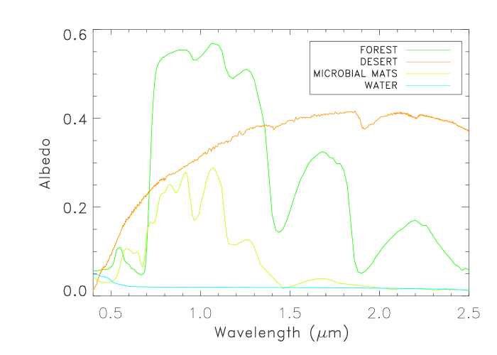
Figure 2: Spectral reflectance of the four surface types used in our model for the Earth 500Ma ago: forest (green), desert (orange), microbial mats (light green) and water (blue).

To carry out our goal of finding out how the appearance of life over land could affect Earth’s reflectance properties, we have considered four different continental land types: water, desert, microbial mats and forest. Figure 2 shows the wavelength-dependent albedos of each surface type according to the ASTER Spectral Library and the USGS Digital Spectral Library.

The continental distribution during the Late Cambrian has been taken from Ron Blakey’s Web site. Surface maps of our planet in that epoch are available online. The Earth geologic information has been regridded into the 64x32 pixel grid used by our model.

2.3 Cloud Distribution and Optical Properties

In our model, the spatial distribution of clouds was taken from the International Satellite Cloud Climatology Project (ISCCP; Rossow et al. 1996) cloud climatology. With the aim of getting information about the global distribution of clouds over different surface types, and in order to reconstruct the possible cloud distribution of the Late Cambrian (500 Ma ago), we have proceeded in the same way as in Sanromá & Pallé (2012) but here, instead of using only the total cloud amount information, we have used information on three separate cloud layers: low (1000-680 Mb), mid (680-440 Mb) and high cloud (440-30 Mb) data.

The optical properties of each cloud type, wavelength-dependent scattering and absorption coefficients, and the asymmetry parameter, were obtained from the Optical Properties of Aerosols and Clouds (OPAC) data base (Hess et al. 1998). We have considered physical cloud thicknesses of 1 km, and we have assumed that the scattering phase function is described by the Henyey-Greenstein equation inside clouds, and by the Rayleigh scattering function outside them.

We calculated the spatial distribution of these three cloud types according to the surface type lying beneath. To perform this classification, we used real geographical information about the different types of surfaces and vegetation in the present Earth, available from the ISCCP Web site. Although the ISCCP classifies the surfaces as water, rain-forest, deciduous-forest, evergreen-forest, grassland, tundra, shrub-land, desert, and ice, we have only distinguished between four surface types: water, desert, ice, and vegetation, where the latest is defined as the sum of rain-forest, deciduous-forest, evergreen-forest, grassland, tundra, or shrub-land. We then computed the mean cloudiness at each latitude point, obtaining the empirical relationships between the amount of clouds, surface type, and latitude for low, mid, and high clouds (see Sanromá & Pallé (2012) for details on the method). These relationships allow us to reconstruct the possible cloudiness distribution of the Earth 500 Ma ago.

It is worth noting that we do not have any empirical information about how clouds behave over extended microbial mat surfaces. Thus in our calculation we have used both the cloudiness information corresponding to deserts and vegetation. Probably the answer is somewhere in between, as microbial mats will increase transpiration and moisture compared to bare land. However, we will show how the choice of cloud amounts does not substantially affect the results.

3 SPECTRA AND LIGHT CURVES OF EARTH 500MA AGO

3.1 Spectral Models

The development of advanced land plants is believed to have taken place during the Late Ordovician, about 450 Ma ago, albeit fungi, algae, and lichens may have greened many land areas long before (Gray et al. 1985). Thus, to determine the impact that such changes could cause in the appearance of the ancient Earth’s spectrum, we have run our model for four separate scenarios. First of all, to illustrate the spectrum properties of a planet without life on its surface, we have considered that the continental crust of the Earth 500 Ma ago was entirely desert. While this might not be entirely true, it certainly was true at some point earlier in Earth’s history, with an unknown continental distribution. Here, we chose to keep the Late Cambrian continental structure in order to isolate the spectral changes due to land scenery changes from those introduced by changing continental distribution (Sanromá & Pallé 2012). Then, we have regarded a case where continents were covered by microbial mats. Here, two separate simulations were run, with the cloud types distribution over land corresponding to desert and to vegetated areas. We have also considered the case where the continental crust during the Late Cambrian was entirely covered by evolved plants, like those that dominate the continental surface today. Finally, in Section 3.2 we have also considered more realistic cases with 50% mixtures between different surface types. In all cases ocean areas remained the same, and a three-layer cloud distribution over the whole planet is applied.

Figure 3 shows synthetic disk-integrated spectra of the Earth 500 Ma ago covering the spectral ranges between 0.4 and 2.5 $\mu$$m$, at different times of the day, for each of our four cases where continents are totally covered by i) deserts, ii) vegetation, iii) microbial mats with the cloudiness information corresponding to deserts, and iv) microbial mats with the clouds corresponding to vegetation. In all cases throughout this paper, the observer and the Sun are both located over the planet’s equator in such a way that the observer is looking at a quarter-illuminated planet (phase angle $90^{\circ}$). For an extrasolar planet, the maximum angular separation from the parent star along the orbit occurs at phase $90^{\circ}$, as defined from the observer’s position. Thus, this is the more relevant geometry for future exoplanet studies.

One can note that as continents come in and out of the field of view, the global Earth’s spectra change. At 8:00 UT, when the continental presence is at maximum, the changes are more dramatic, in contrast to the spectra at 18:00 UT where differences between the four scenarios cannot be appreciated. That is related with the percentage of land that were illuminated and visible at each time. These percentages are approximately 24%, 46%, 36%, and 6% for 4:00, 8:00, 12:00, and 18:00 UT, respectively.

In order to show such intensity changes in terms of the strength of the vegetation’s red-edge, we have calculated the ratio between the 0.740-0.750 $\mu$$m$ and the 0.678-0.682 $\mu$$m$ spectral ranges (Table 1). The choice of these spectral regions was made according to Montañés-Rodríguez et al. (2006). As expected, at 18:00 UT (6% of land) this rate is almost the same in our four cases, while at 08:00 UT (46% of land) the maximum is reached in the vegetation case where the red-edge is more pronounced.

For a planet covered by bare dirt, Figure 3 illustrates some diurnal temporal variability, which is small in the visible range, but increases toward redder wavelengths. Gómez-Leal et al. (2012) studied the mid-IR emission of the planet in order to derive the rotational period. They found that the signature of the emission from the Sahara desert, among other, can be seen from space and determines a clear maximum in emission. Thus, it is probable that this variability would be even larger in the mid-IR.

In the case of a planet with continents covered by microbial mats, the spectra do not seem to vary much along the planet rotation, despite the fact of having a large and well differentiated land mass. The impact of using two different clouds layers in the model (desert or vegetation) is almost negligible, being the former just a little bit more variable.

On the contrary the spectrum of a planet covered entirely by plants varies significantly along the day, with the maximum variance occurring in the visible and near-IR. In particular the variability along the red-edge feature (at 700 $nm$) is large, and it extends all the way into the near-IR.

3.2 Photometric Light-Curves

Observing a detailed reflectance spectrum of an exoplanet would no doubt be a major advantage toward characterizing its atmospheric composition and surface features. However, given the low signal to noise ratio scenarios that are expected for such observations, spectral information might be difficult to retrieve, especially at high enough temporal resolution to allow sampling of the planet’s rotation. Broadband photometric observations are perhaps a more realistic scenario. In order to simulate such photometric observations, we have convolved our modeled spectra with standard visible and near-infrared photometric filters, namely, B,V, R, I, z, J, H, and K.

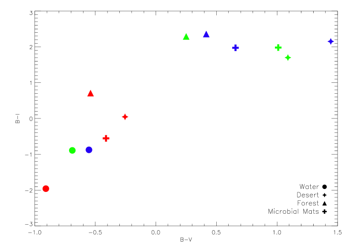
Figure 4: Color-color diagram of homogeneous test planets. Symbols denote planets whose surface is totally covered by water (circles), deserts (stars), vegetation (triangles), and microbial mats (crosses). The values are shown for atmosphere-less planets (this work in blue and Hegde & Kaltenegger 2013 in green), and for planets with an earth-like atmosphere (red). Notice that adding an atmosphere to the model reduces considerably the variability of the colors of the different planets.

Figure 4 shows the B-V versus B-I color-color diagram of test planets fully covered by one specific surface type, i.e., planets totally covered by water, desert, vegetation, and microbial mats, with and without atmosphere (blue and red symbols, respectively). As can be seen, the addition of an atmosphere in our models moves the position of the planets in the color-color diagram significantly, reducing the color spread of the different surface types along the diagram.

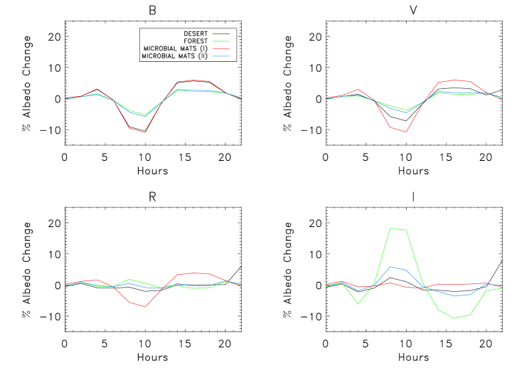
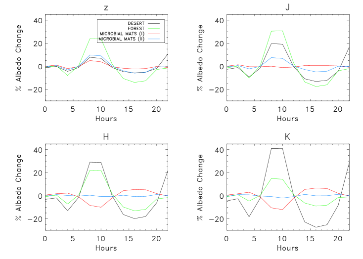
Figure 5: Diurnal light curves of the Earth for the four scenarios contemplated in this paper. The y-scale is the same for all standard photometric filters. The light curves represent the percentage of the albedo change along a day for the 4 scenarios.

Figure 5 shows the photometric time-dependent variations in the disk-integrated reflected light along one day. The rotational light curves are plotted for our four scenarios, and for each photometric filter. For the Johnson visible system filters, these light-curves show a relatively smooth shape, with the four scenarios being quite similar one to another, and with albedo changes lower than 6% in general. The only noticeable signature is the enhancement in brightness, about 20%, in the I filter, for the vegetated case (green line) between 6 and 12 UT. This is again related to the vegetation’s signature, the red-edge, since the main continental mass is in full view (and illuminated by the Sun) at this time.

More interesting results are obtained when one moves redward (bottom part of Figure 5). The diurnal light curves of a planet with bare desert surfaces (black line) in J, H and K filters show a considerable increase in brightness between 6 and 12 UT of about 20%, 30% and 40% respectively, making immediately obvious the existence of a continent. The same is found in the vegetation case (green line), being these variability of around 30%, 20% and 15% for J, H and K, respectively.

The light curve for a planet with continents covered with microbial mats with cloudiness distribution corresponding to vegetation (blue line) is very mutted, with little variability in either the visible or the near-IR spectral ranges. In contrast, light curves of the microbial mats case with cloudiness distribution corresponding to desert (red line) show a decrease in the albedo of around 10% in the H, and K filters, when the main continental mass is facing the observer. In the J filter these light curves do not exhibit any variation, making it impossible to even discern the presence of continental masses.

Figure 6 shows the amplitude of albedo variability of each of the studied cases as a function of the different photometric filters. As considering continents completely covered by just only one surface type might not be very realistic, we have also analyzed cases where continents were covered by patchy microbial mats, desert and vegetation. As an example, in Figure 6 we present the results obtained for: i) continental masses irregularly covered by $50\%$ deserts and $50\%$ microbial mats, and ii) for continents unevenly covered by $50\%$ vegetation and $50\%$ microbial mats.

The curves in Figure 6 show a distinctive shape depending on surface type. When continents are completely covered by deserts (black line) the amplitude of albedo change increases rapidly when one moves from z filter redward, while the variability is nearly constant in the visible. When continents are totally covered by vegetation (green line), that albedo variability increases nearly monotonously from R filter to J filter, where it peaks, and then decreases redward. In contrast to these two cases, when continents are covered by microbial mats (blue and red lines), the amplitude of albedo change is not strongly dependent on the filter selected and is much more mutted. Moreover, when we considered that the Earth 500 Ma ago had continents covered by a mixture of microbial mats and deserts/vegetation (yellow and light-blue lines), the shape of these amplitude variability curves resembles the typical shape of the desert/vegetated cases, but with muted variability.

At the light of these results we conclude that it should be a priori possible to determine the type of continental surface on a rocky Earth-like planet based on color photometry and given a high enough signal-to-noise ratio. A planet covered by bare desert areas will have a large diurnal variability in the J, H and K bands. While this is also the case for vegetated continents, in this case an additional bump in the I band is to be expected, which would be missing in a desert planet. Furthermore, the hypothesis of deserted continents could be further tested/confirmed by observations in the mid-IR photometric bands (Gómez-Leal et al. 2012).

In the case of a planet with extended microbial mats, its nature would be determined by the detection of the presence of continents by using the light curves in B and V bands, and then finding a lower than expected percentage variability in the J, H and K bands, with the reflection peak characteristics of plants and deserts missing.

Although not shown in this work, we also studied the same scenarios but with cloud-free atmospheres. As expected, we find that the omission of clouds decreases the amount of reflected light in comparison to the respective non-clear sky condition. Nevertheless, daily variations in the disk-integrated spectra become more dramatic in the cloud-free case than in the cloudy one. These cases, however, are highly unrealistic.

4 CONCLUSIONS

In this paper we have used a radiative transfer code to simulate the globally-integrated spectral variability of the Earth 500 Ma ago, using four possible scenarios regarding the continental surface properties. Our simulations also include realistic distributions of clouds over the whole planet at three altitude layers. We find that as the continental surface changes from desert ground to microbial mats and to land plants, it produces detectable changes in the globally-averaged Earth’s reflectance that vary substantially as the Earth rotates. By binning the data into standard astronomical photometric band we see that the variability of each surface type is located in different bands and can induce reflectance changes of up to 40% in periods of hours. We conclude that using photometric observations of an Earth-like planet at different photometric bands, it would be possible to discriminate between bare continental surfaces, large microbial mats extensions, or plant-covered continents. While in the recent literature the red edge feature of vegetation at visible wavelengths has been proposed as a signature for land plants, observations in near-IR bands can be equally suited for this purpose.

Figure 3: Earth’s reflectance 500 Ma ago, taken as $\pi$ times the disk-averaged radiance divided by the solar flux, in the VIS-NIR, for our four cases in which the continents are covered by: deserts, vegetation, microbial mats with the cloudiness information corresponding to desert (I), and microbial mats with the cloudiness information corresponding to vegetation (II). The Earth is viewed at a phase angle of 90^∘ and the different spectra follow their diurnal rotation. Both, the observer and the Sun are located over the equator. The spectra have been smoothed with a 100 point running mean for illustration purposes.

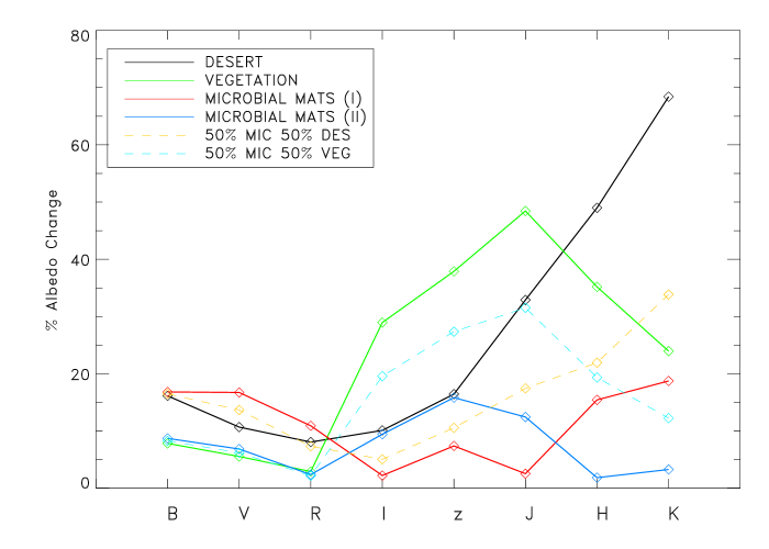
Figure 6: Amplitude of the albedo variability as a function of the standard photometric filters. Colors represent the different cases studied here: the Earth 500 Ma ago with continents completely covered by deserts (black solid line), by vegetation (green solid line), by microbial mats (red and blue solid lines) and covered by a mixture of surface types: 50% microbial mats - 50% deserts (yellow dashed line), and 50% microbial mats - 50% vegetation (blue dashed line).

Table 1: The diurnal variability of the vegetation’s red edge strenght for the Earth 500 Ma ago.

Surface Type	2 UT	8 UT	12 UT	18 UT
Desert	1.14	1.35	1.16	1.03
Forest	1.03	1.05	1.03	1.01
Microbial Mats (I)	1.05	1.12	1.05	1.02
Microbial Mats (II)	1.04	1.10	1.05	1.02

References

- Arnold et al. (2002) Arnold, L., Gillet, S., Lardière, O., Riaud, P., & Schneider, J. 2002, A&A, 392, 231
- Borucki et al. (2012) Borucki, W. J., Koch, D. G., Batalha, N., et al. 2012, ApJ, 745, 120
- Cassan et al. (2012) Cassan, A., Kubas, D., Beaulieu, J.-P., et al. 2012, Nature, 481, 167
- Charbonneau et al. (2009) Charbonneau, D., Berta, Z. K., Irwin, J., et al. 2009, Nature, 462, 891
- Cockell et al. (2009) Cockell, C. S., Kaltenegger, L., & Raven, J. A. 2009, Astrobiology, 9, 623
- Cowan et al. (2009) Cowan, N. B., Agol, E., Meadows, V. S., et al. 2009, ApJ, 700, 915
- Cowan et al. (2011) Cowan, N. B., Robinson, T., Livengood, T. A., et al. 2011, ApJ, 731, 76
- Fressin et al. (2012) Fressin, F., Torres, G., Rowe, J. F., et al. 2012, Nature, 482, 195
- Fujii & Kawahara (2012) Fujii, Y. & Kawahara, H. 2012, ApJ, 755, 101
- Gallery et al. (1983) Gallery, W. O., Kneizys, F. X., & Clough, S. A. 1983, AFGL-TR-0208 Environemental Research papers, 83, 0065
- García Muñoz & Pallé (2011) García Muñoz, A. & Pallé, E. 2011, J. Quant. Spec. Radiat. Transf., 112, 1609
- García Muñoz et al. (2012) García Muñoz, A., Zapatero Osorio, M. R., Barrena, R., et al. 2012, ApJ, 755, 103
- Gómez-Leal et al. (2012) Gómez-Leal, I., Pallé, E., & Selsis, F. 2012, ApJ, 752, 28
- Goode et al. (2001) Goode, P. R., Qiu, J., Yurchyshyn, V., et al. 2001, Geophys. Res. Lett., 28, 1671
- Gray et al. (1985) Gray, J., Chaloner, W., & Westoll, T. 1985, Phil. Trans. R. Soc., 309, 167
- Hamdani et al. (2006) Hamdani, S., Arnold, L., Foellmi, C., et al. 2006, A&A, 460, 617
- Hart (1978) Hart, M. H. 1978, Icarus, 33, 23
- Hegde & Kaltenegger (2013) Hegde, S. & Kaltenegger, L. 2013, Astrobiology, 13, 47
- Hess et al. (1998) Hess, M., Koepke, P., & Schult, I. 1998, Bull. Am. Met. Soc., 79, 831
- Kaltenegger et al. (2007) Kaltenegger, L., Traub, W. A., & Jucks, K. W. 2007, ApJ, 658, 598
- Kasting & Siefert (2002) Kasting, J. F. & Siefert, J. L. 2002, Science, 296, 1066
- Kawahara & Fujii (2010) Kawahara, H. & Fujii, Y. 2010, ApJ, 720, 1333
- Kawahara & Fujii (2011) Kawahara, H. & Fujii, Y. 2011, ApJ, 739, L62
- Kiang et al. (2007a) Kiang, N. Y., Segura, A., Tinetti, G., et al. 2007a, Astrobiology, 7, 252
- Kiang et al. (2007b) Kiang, N. Y., Siefert, J., Govindjee, & Blankenship, R. E. 2007b, Astrobiology, 7, 222
- Montañés-Rodríguez et al. (2006) Montañés-Rodríguez, P., Pallé, E., Goode, P. R., & Martín-Torres, F. J. 2006, ApJ, 651, 544
- Muirhead et al. (2012) Muirhead, P. S., Johnson, J. A., Apps, K., et al. 2012, ApJ, 747, 144
- Oakley & Cash (2009) Oakley, P. H. H. & Cash, W. 2009, ApJ, 700, 1428
- Pallé et al. (2008) Pallé, E., Ford, E. B., Seager, S., Montañés-Rodríguez, P., & Vazquez, M. 2008, ApJ, 676, 1319
- Pallé et al. (2004) Pallé, E., Goode, P. R., Montañés-Rodríguez, P., & Koonin, S. E. 2004, Science, 304, 1299
- Pallé et al. (2003) Pallé, E., Goode, P. R., Yurchyshyn, V., et al. 2003, J. Geophys. Res. (Atmos.), 108, 4710
- Pepe et al. (2011) Pepe, F., Lovis, C., Ségransan, D., et al. 2011, A&A, 534, A58
- Qiu et al. (2003) Qiu, J., Goode, P. R., Pallé, E., et al. 2003, J. Geophys. Res. (Atmos.), 108, 4709
- Robinson et al. (2011) Robinson, T. D., Meadows, V. S., Crisp, D., et al. 2011, Astrobiology, 11, 393
- Rossow et al. (1996) Rossow, W. B., Walker, A. W., Beuschel, D. E., & Roiter, M. D. 1996, World Climate Research Programme Report WMO/TD 737 (Geneva, Switzerland: World Meteorological Organization
- Rothman et al. (2009) Rothman, L. S., Gordon, I. E., Barbe, A., et al. 2009, J. Quant. Spec. Radiat. Transf., 110, 533
- Sanromá & Pallé (2012) Sanromá, E. & Pallé, E. 2012, ApJ, 744, 188
- Seager et al. (2005) Seager, S., Turner, E. L., Schafer, J., & Ford, E. B. 2005, Astrobiology, 5, 372
- Seckbach & Oren (2010) Seckbach, J. & Oren, A. 2010, Microbial Mats: Modern and Ancient Microorganisms in Stratified Systems, Cellular Origin, Life in Extreme Habitats and Astrobiology (Springer London, Limited)
- Stammnes et al. (1988) Stammnes, K., Tsay, S. C., Wiscombre, W., & Jayaweera, K. 1988, Appl. Opt., 27, 2502
- Sterzik et al. (2012) Sterzik, M. F., Bagnulo, S., & Palle, E. 2012, Nature, 483, 64
- Tinetti et al. (2006a) Tinetti, G., Meadows, V. S., Crisp, D., et al. 2006a, Astrobiology, 6, 34
- Tinetti et al. (2006b) Tinetti, G., Meadows, V. S., Crisp, D., et al. 2006b, Astrobiology, 6, 881
- Tinetti et al. (2006c) Tinetti, G., Rashby, S., & Yung, Y. L. 2006c, ApJ, 644, L129
- Turnbull et al. (2006) Turnbull, M. C., Traub, W. A., Jucks, K. W., et al. 2006, ApJ, 644, 551
- Udry et al. (2007) Udry, S., Fischer, D., & Queloz, D. 2007, Protostars and Planets V, 685
- Woolf et al. (2002) Woolf, N. J., Smith, P. S., Traub, W. A., & Jucks, K. W. 2002, ApJ, 574, 430