Asymmetric Langevin dynamics for the ferromagnetic spherical model

Abstract

The present work pursues the investigation of the role of spatial asymmetry and irreversibility on the dynamical properties of spin systems. We consider the ferromagnetic spherical model with asymmetric linear Langevin dynamics. Such an asymmetric dynamics is irreversible, i.e., breaks detailed balance, because the principle of action and reaction is violated. The fluctuation-dissipation theorem therefore no longer holds. The stationary state is however still Gibbsian, i.e., the weights of configurations are given by the Boltzmann factor corresponding to the ferromagnetic Hamiltonian. The model is exactly solvable in any dimension, enabling an analytical evaluation of time-dependent observables. We show the existence of two regimes of violation of the fluctuation-dissipation theorem in the nonequilibrium stationary state: a regime of weak violation where the stationary fluctuation-dissipation ratio is finite but less than unity and varies continuously with the asymmetry, and a regime of strong violation where the fluctuation-dissipation ratio vanishes asymptotically. This phenomenon was first uncovered in the asymmetric kinetic Ising chain. The present results suggest that this novel kind of dynamical transition in nonequilibrium stationary states might be quite general. We also perform a systematic analysis of several regimes of interest, either stationary or transient, in various dimensions and in the different phases of the model.

,

1 Introduction

In the past decades many studies have been devoted to the dynamics of ferromagnetic spin systems. If such a system is quenched from a disordered initial state, it relaxes, at high temperature, towards its paramagnetic equilibrium state, whereas, in the low-temperature ordered phase, equilibrium is never reached and the system undergoes a non-stationary coarsening process [1].

Both situations are illustrated by the exactly solvable Glauber-Ising chain [2]. At finite temperature, where the relaxation time is finite, the convergence to the paramagnetic equilibrium state can be monitored by the exact determination of the two-spin correlation functions, either for equal or unequal times. When the system has reached equilibrium, its response to a small perturbation is simply related to the two-time correlation function, which is the content of the fluctuation-dissipation theorem [2]. In the low-temperature regime, where the relaxation time is diverging, the system undergoes coarsening, with scaling and universality properties which have been characterized in more recent studies [1, 3, 4, 5, 6]. In higher dimensions, since no exact result prevails, the present understanding of the properties of kinetic Ising models has been achieved by numerical simulations, scaling arguments and field-theoretical methods [1].

For kinetic Ising models with non conserved (Glauber) dynamics, a line of investigation which has been almost completely overlooked until recently is the role of spatial asymmetry in the dynamics. This is in contrast with the case of Ising models with conserved (Kawasaki) dynamics in the presence of a bias due to an external field, which have been thoroughly investigated, mostly numerically [7]. In the context of Glauber dynamics, asymmetry means that the flipping spin is not equally influenced by all its neighbours. Such an asymmetric dynamics is therefore irreversible, because the principle of action and reaction is violated and detailed balance no longer holds. In a recent past, two studies have been devoted to Ising models with non conserved asymmetric dynamics [8, 9]. Reference [8] gives examples of rate functions for the kinetic Ising model in one and two dimensions with totally asymmetric dynamics leading to a Gibbsian stationary state (in the sense that the weights of configurations are given by the Boltzmann factor corresponding to the ferromagnetic Hamiltonian). Reference [9] investigates, by numerical means, the possible existence of a phase transition for the kinetic Ising model, in dimensions two to five, when the usual heat-bath rate is modified by truncating the local field, keeping a subset of influential spins only. The dynamics thus obtained neither fulfills detailed balance, nor global balance (with respect to the ferromagnetic Hamiltonian), and therefore leads to an unknown stationary state, except in low dimension, where the problem can be easily analyzed [10].

The works [8, 9] motivated the systematic study presented in [10]. In particular, the examples given by Künsch [8] raised the following questions: To what extent are these examples unique? Can they be extended to lattices in dimension higher than two? As demonstrated in [10], as long as the dynamics is not totally asymmetric, the space of parameters defining the rate function of irreversible Gibbsian Ising models in one and two dimensions is large. However, imposing total asymmetry of the dynamics yields a unique solution (up to a global time scale), for all the examples considered (linear chain, square and triangular lattices). The answer to the second question is presumably negative: there is no such Gibbsian irreversible dynamics for the cubic lattice and one can argue that there are neither totally asymmetric Gibbsian dynamics for lattices of coordination $z\geq 8$ [10].

Such Gibbsian asymmetric kinetic models, where the flipping spin is not equally influenced by all its neighbours, provide benchmarks to study the physical consequences of irreversibility, in particular the properties of the resulting nonequilibrium stationary state. For instance, for the Ising chain, a one-parameter family of asymmetric dynamics can been shown to keep the exact solvability of the symmetric Glauber dynamics, allowing a detailed analysis of its dynamical features [11]. One of the most striking results is the existence of two regimes of violation of the fluctuation-dissipation theorem in the nonequilibrium stationary state: when the asymmetry parameter is less than a threshold value, there is weak violation of the fluctuation-dissipation theorem, with a finite asymptotic fluctuation-dissipation ratio, whereas this ratio vanishes above the threshold [11]. At low temperature, the asymptotic fluctuation-dissipation ratio depends on the strength of the asymmetry [3], and in particular vanishes at long times, as soon as the asymmetry is present, while in the absence of asymmetry it takes a universal value equal to $1/2$ [3]. For the two-dimensional Ising model with the asymmetric dynamics introduced in [10] numerical simulations show many features in common with the one-dimensional case, in particular the existence of two regimes of violation of the fluctuation-dissipation theorem [12]. Irreversibility also implies a non-vanishing entropy production rate in the stationary state, which can be exactly computed for irreversible Gibbsian Ising models since the stationary measure is known [13, 14].

In the present work we pursue the investigation of the role of spatial asymmetry and irreversibility on the dynamics of spin systems, by considering the ferromagnetic spherical model with asymmetric Langevin dynamics. We follow the thread of our earlier investigations of the spherical model with symmetric Langevin dynamics [15] and of the asymmetric kinetic Ising chain [11]. The outcomes of the present study turn out to share many common features with those of the latter reference. In particular we show that the phenomenon described above of two regimes of violation of the fluctuation-dissipation theorem in the stationary state also exists for the spherical model, in any dimension, and thereby acquires a status of greater generality.

The spherical model has been introduced long ago by Berlin and Kac [16], as an attempt to simplify the Ising model. It is also known to be equivalent to the $n\to\infty$ limit of the $\mbox{O}(n)$ Heisenberg model [17]. Its thermodynamic properties can be studied exactly in any dimension. The model however possesses non-trivial critical properties [16, 18]. The spherical model has another significant advantage in the present context: its time-dependent properties under symmetric Langevin dynamics can be investigated by analytical means, in all the phases of the model and in any dimension [19, 20, 21, 22, 15]. Other aspects of the dynamics of the spherical model have been explored, such as the presence of a constant magnetic field, long-range or competing interactions, finite-size and surface effects, a temperature-dependent bath, and a correlated initial state [23]. The dynamics of spherical spin-glass models has also received much attention, especially in the mean-field geometry [24].

The spherical model with asymmetric dynamics has also been considered in previous studies. One should first mention the study of the dynamics of a mean-field spherical spin glass with random asymmetric bonds [25], inspired by neuronal networks with asymmetric synaptic couplings. More recently, Langevin dynamics for the ferromagnetic spherical model with an asymmetry has been considered in [26]. The latter work was however limited to an evaluation of the entropy production rate in the stationary state. Instead, the main focus of the present work is on the dynamical properties of the model, at stationarity or out of stationarity, in particular through an investigation of the two-time sector of the dynamics, and especially of the fluctuation-dissipation ratio.

The setup of the paper is as follows. The spatially asymmetric linear Langevin dynamics is introduced in section 2, and shown to be characterized by a velocity vector ${{\bf V}}$. In section 3 we show why the nonequilibrium stationary state reached by this dynamics is Gibbsian, in the sense that the weights of configurations are the Boltzmann weights corresponding to the ferromagnetic Hamiltonian. We also give a reminder of some features and properties necessary for the sequel: critical temperature, relaxation time, equal-time correlations. In section 4 we derive general expressions for dynamical quantities in the two-time sector. As the dynamics is irreversible for any non-zero ${{\bf V}}$, the fluctuation-dissipation theorem relating the two-time correlation and response functions no longer holds, even in the stationary state. We derive a few properties of the nonequilibrium stationary state in section 5, including the dispersion of the fluctuation-dissipation ratio in Fourier space and the entropy production rate. We then show that there exist two distinct regimes of violation of the fluctuation-dissipation theorem: a regime of weak violation at small ${{\bf V}}$, where the stationary fluctuation-dissipation ratio is finite but less than unity, and a regime of strong violation at large ${{\bf V}}$, where the fluctuation-dissipation ratio falls off exponentially with time. This is demonstrated in one dimension (section 6) and in higher dimension (section 7). The next three sections contain a detailed investigation of the transient properties of the model, before the nonequilibrium stationary state sets in. We successively consider the low-temperature scaling regime of the one-dimensional model (section 8) and the vicinity of the critical point in higher dimension, where a continuum description makes the analysis simpler, both in the classical regime ($D>4$) in section 9 and in the non-classical one ($2<D<4$) in section 10. In all these situations, the effect of an asymmetry on the dynamical critical properties of the model bears strong similarities with the case of the asymmetric kinetic Ising chain. The fluctuation-dissipation ratio has a scaling form in two variables, respectively related to the temperature difference $T-T_{c}$ and to the asymmetry parameter ${{\bf V}}$. Finally, the asymmetric dynamics of the low-temperature ferromagnetic phase is investigated in section 11; it exhibits two successive regimes (beta and alpha), in agreement with the phenomenology of glassy physics. The quantitative behavior of the two-time correlation function and of the corresponding fluctuation-dissipation ratio is shown to be affected by the irreversibility of the dynamics.

2 The model

The definition of the ferromagnetic spherical model is well known. Consider a lattice in arbitrary dimension $D$, chosen to be hypercubic for simplicity. The spins $S_{\bf x}$, sitting at the vertices ${\bf x}$, are real variables obeying the spherical constraint

$$\sum_{\bf x}S_{\bf x}^{2}=N,$$ (2.1)

where $N$ is the number of spins in the system, which is supposed to be finite for the time being. The Hamiltonian of the model reads

$${\cal H}=-\sum_{({\bf x},{\bf y})}S_{\bf x}S_{\bf y},$$ (2.2)

where the sum runs over pairs of neighboring sites.

We first remind the rules of the symmetric Langevin dynamics, before addressing the case of asymmetric dynamics, which is the focus of the paper.

2.1 Reversible (symmetric) Langevin dynamics

Hereafter we assume that the system is homogeneous, i.e., invariant under spatial translations. This holds for a finite sample with periodic boundary conditions, and for the infinite system. Furthermore, along the lines of earlier studies of dynamical properties, we shall consider the mean spherical model, where the constraint (2.1) is imposed on average, becoming thus the mean spherical constraint [27]:

$$\langle S_{\bf x}(t)^{2}\rangle=1.$$ (2.3)

Throughout the following, we consistently use the notations of [15].

Symmetric Langevin dynamics is defined by the stochastic differential equation

$$\frac{{\rm d}S_{\bf x}}{{\rm d}t}=F_{\bf x}-\lambda(t)S_{\bf x}+\eta_{\bf x}(t),$$ (2.4)

where $\eta_{\bf x}(t)$ is a Gaussian white noise with covariance

$$\langle\eta_{\bf x}(t)\eta_{\bf y}(t^{\prime})\rangle=2T\,\delta_{{\bf x},{\bf y}}\,\delta(t-t^{\prime}),$$ (2.5)

and $\lambda(t)$ is a Lagrange multiplier ensuring the constraint (2.3) at any time $t$. We choose for convenience to parametrize $\lambda(t)$ as

$$\lambda(t)=2D+z(t).$$ (2.6)

Finally, $F_{\bf x}$ is the force exerted on $S_{\bf x}$ by the other spins, i.e.,

$$F_{\bf x}=-\frac{\partial{\cal H}}{\partial S_{\bf x}}=\sum_{a=1}^{D}(S_{{\bf x}-{\bf e}_{a}}+S_{{\bf x}+{\bf e}_{a}}),$$ (2.7)

where the $2D$ neighbors of ${\bf x}$ are ${\bf y}={\bf x}\pm{\bf e}_{a}$, and ${\bf e}_{a}$ is a unit vector in direction $a=1,\dots,D$. The Langevin equation (2.4) thus reads

$$\frac{{\rm d}S_{\bf x}}{{\rm d}t}=\sum_{a=1}^{D}(S_{{\bf x}-{\bf e}_{a}}+S_{{\bf x}+{\bf e}_{a}}-2S_{\bf x})-z(t)S_{\bf x}+\eta_{\bf x}(t).$$ (2.8)

This dynamics is reversible and obeys detailed balance with respect to the Hamiltonian (2.2) at any temperature $T$; it drives the spherical model to the corresponding equilibrium state, at least in the paramagnetic phase ($T>T_{c}$).

2.2 Irreversible (asymmetric) Langevin dynamics

We define the most general asymmetric Langevin dynamics by dissymetrizing the roles of the ‘left’ neighbors (${\bf y}={\bf x}-{\bf e}_{a}$) and of the ‘right’ neighbors (${\bf y}={\bf x}+{\bf e}_{a}$), while keeping the linearity of the Langevin equation. We are thus led to deform the expression (2.7) of the force $F_{\bf x}$ into

$$\widehat{F}_{\bf x}=\sum_{a=1}^{D}\bigl{(}(1+V_{a})S_{{\bf x}-{\bf e}_{a}}+(1-V_{a})S_{{\bf x}+{\bf e}_{a}}\bigr{)},$$ (2.9)

where $V_{a}$ are arbitrary parameters. From now on, the vector ${{\bf V}}$ with components $V_{a}$ will be interpreted as a velocity.

Asymmetric Langevin dynamics is therefore defined by the linear equation

$$\frac{{\rm d}S_{\bf x}}{{\rm d}t} = \sum_{a=1}^{D}\bigl{(}(1+V_{a})S_{{\bf x}-{\bf e}_{a}}+(1-V_{a})S_{{\bf x}+{\bf e}_{a}}-2S_{\bf x}\bigr{)}$$ (2.10)

$$- z(t)S_{\bf x}+\eta_{\bf x}(t).$$

This dynamics is irreversible, i.e., does not obey detailed balance. It however drives the system to a Gibbsian nonequilibrium stationary state, where the weights of spin configurations are the Boltzmann weights associated with the Hamiltonian (2.2) at temperature $T$, irrespective of the velocity ${{\bf V}}$. This will be proved in section 3.1.

3 One-time observables

3.1 Equal-time correlation function

From now on, we consider the thermodynamic limit of an infinite system. We assume that the initial state is the infinite-temperature equilibrium state with the mean spherical constraint (2.3). The spins $S_{\bf x}(0)$ at time $t=0$ are therefore independent and identically distributed Gaussian variables with unit variance. The linearity of the Langevin equation (2.10) ensures that the spins $S_{\bf x}(t)$ remain Gaussian at any time $t$. The only non-trivial one-time observable is therefore the equal-time two-point correlation function

$$C_{{\bf x}-{\bf y}}(t)=\langle S_{\bf x}(t)S_{\bf y}(t)\rangle,$$ (3.1)

where brackets denote an average over the infinite-temperature initial state and over thermal histories (realizations of the noise).

The main result of this section is as follows. The equal-time correlation function, whose explicit expression is given in (3.13), does not depend on ${{\bf V}}$. It therefore coincides with the equal-time correlation function for symmetric Langevin dynamics.

Hereafter we only summarize the main properties of this correlation function, referring the reader to [15] for more details. We have

$$C_{\bf 0}(t)=1,$$ (3.2)

reflecting the mean spherical constraint (2.3), and

$$C_{\bf x}(0)=\delta_{{\bf x},{\bf 0}},$$ (3.3)

as a consequence of the statistical independence of the spins in the initial state.

In order to pursue with the explicit evaluation of the correlation function $C_{\bf x}(t)$, we have to first solve the Langevin equation (2.10) for an infinite system. This can be readily done in Fourier space. Define the Fourier transform by the formulas

$$f^{\rm F}({\bf q})=\sum_{\bf x}f_{\bf x}\,{\rm e}^{-{\rm i}{\bf q}.{\bf x}},\qquad f_{\bf x}=\int\!{\frac{{\rm d}^{D}{\bf q}}{(2\pi)^{D}}}\,f^{\rm F}({\bf q})\,{\rm e}^{{\rm i}{\bf q}.{\bf x}},$$ (3.4)

where

$$\int\!{\frac{{\rm d}^{D}{\bf q}}{(2\pi)^{D}}}=\int_{-\pi}^{\pi}\frac{{\rm d}q_{1}}{2\pi}\cdots\int_{-\pi}^{\pi}\frac{{\rm d}q_{D}}{2\pi}$$ (3.5)

is the normalized integral over the first Brillouin zone. Equation (2.10) thus becomes

$$\frac{\partial S^{\rm F}({\bf q},t)}{\partial t}=-[\Omega({\bf q})+z(t)]S^{\rm F}({\bf q},t)+\eta^{\rm F}({\bf q},t),$$ (3.6)

where

$$\Omega({\bf q})=2\sum_{a=1}^{D}(1-\cos q_{a}+{\rm i}V_{a}\sin q_{a})$$ (3.7)

and

$$\langle\eta^{\rm F}({\bf q},t)\eta^{\rm F}({\bf q}^{\prime},t^{\prime})\rangle=2T\,(2\pi)^{D}\,\delta^{D}({\bf q}+{\bf q}^{\prime})\,\delta(t-t^{\prime}).$$ (3.8)

The solution to (3.6) reads

$$S^{\rm F}({\bf q},t) = {\rm e}^{-\Omega({\bf q})t-Z(t)}$$ (3.9)

$$\times \left(S^{\rm F}({\bf q},0)+\int_{0}^{t}{\rm d}s\,{\rm e}^{\Omega({\bf q})s+Z(s)}\eta^{\rm F}({\bf q},s)\right),$$

with

$$Z(t)=\int_{0}^{t}{\rm d}s\,z(s).$$ (3.10)

The equal-time correlation function $C^{\rm F}({\bf q},t)$ in Fourier space is defined by

$$\langle S^{\rm F}({\bf q},t)S^{\rm F}({\bf q}^{\prime},t)\rangle=(2\pi)^{D}\delta^{D}({\bf q}+{\bf q}^{\prime})\,C^{\rm F}({\bf q},t).$$ (3.11)

By averaging the expression (3.9) over the white noise $\eta^{\rm F}({\bf q},t)$, whose variance is given by (3.8), and using the initial condition

$$C^{\rm F}({\bf q},0)=1$$ (3.12)

implied by (3.3), we obtain the expression

$$C^{\rm F}({\bf q},t)=\frac{{\rm e}^{-2\omega({\bf q})t}}{g(t)}\left(1+2T\!\int_{0}^{t}{\rm d}s\,{\rm e}^{2\omega({\bf q})s}g(s)\right),$$ (3.13)

where

$$\omega({\bf q})=\frac{1}{2}(\Omega({\bf q})+\Omega(-{\bf q}))=2\sum_{a=1}^{D}(1-\cos q_{a})$$ (3.14)

and

$$g(t)={\rm e}^{2Z(t)}.$$ (3.15)

The expression (3.14) for $\omega({\bf q})$ is independent of the velocity ${{\bf V}}$. We have thus completed the proof of the result announced above, namely that the equal-time correlation function (3.13) is independent of ${{\bf V}}$. As a consequence, one-time observables are identical for symmetric (reversible) and for asymmetric (irreversible) dynamics. This striking property relies fundamentally on the linearity of the Langevin equation.

3.2 Relaxation time and phase diagram

We proceed with the calculation of the relaxation time of the dynamics. The Lagrange multiplier $z(t)$, and thereby the function $g(t)$, are yet to be determined from the constraint (3.2), i.e.,

$$\int\!{\frac{{\rm d}^{D}{\bf q}}{(2\pi)^{D}}}\,C^{\rm F}({\bf q},t)=1.$$ (3.16)

This identity yields a Volterra integral equation [21, 15] for $g(t)$,

$$g(t)=f(t)+2T\!\int_{0}^{t}{\rm d}s\,f(t-s)g(s),$$ (3.17)

with

$$f(t)=\int\!{\frac{{\rm d}^{D}{\bf q}}{(2\pi)^{D}}}\,{\rm e}^{-2\omega({\bf q})t}=\left({\rm e}^{-4t}I_{0}(4t)\right)^{D}\mathrel{\mathop{\approx}\limits_{t\to\infty}}(8\pi t)^{-D/2},$$ (3.18)

where

$$I_{n}(z)=\int\frac{{\rm d}q}{2\pi}\,{\rm e}^{z\cos q+{\rm i}nq}$$ (3.19)

is the modified Bessel function. In Laplace space, (3.17) yields

$$g^{\rm L}(p)=\frac{f^{\rm L}(p)}{1-2Tf^{\rm L}(p)},$$ (3.20)

with

$$f^{\rm L}(p)=\int_{0}^{\infty}{\rm d}t\,f(t)\,{\rm e}^{-pt}=\int\!{\frac{{\rm d}^{D}{\bf q}}{(2\pi)^{D}}}\,\frac{1}{p+2\omega({\bf q})}.$$ (3.21)

The latter function has a branch point at $p=0$, with a singular part of the form

$$f^{\rm L}_{\rm sg}(p)\mathrel{\mathop{\approx}\limits_{p\to 0}}(8\pi)^{-D/2}\Gamma(1-D/2)p^{(D-2)/2},$$ (3.22)

as well as a regular part of the form

$$f^{\rm L}_{\rm reg}(p)=A_{1}-A_{2}p+A_{3}p^{2}+\cdots,$$ (3.23)

where the integrals

$$A_{k}=\int\!{\frac{{\rm d}^{D}{\bf q}}{(2\pi)^{D}}}\,\frac{1}{(2\omega({\bf q}))^{k}}$$ (3.24)

are convergent for $D>2k$. Equations (3.22) and (3.23) jointly determine the small-$p$ behavior of $f^{\rm L}(p)$, as a function of dimension $D$:

$$D<2: \ f^{\rm L}(p)\approx(8\pi)^{-D/2}\Gamma(1-D/2)p^{-(1-D/2)},$$ (3.25)

$$2<D<4: \ f^{\rm L}(p)\approx A_{1}-(8\pi)^{-D/2}|\Gamma(1-D/2)|p^{(D-2)/2},$$ (3.26)

$$D>4: \ f^{\rm L}(p)\approx A_{1}-A_{2}p.$$ (3.27)

Whenever $D=2,4,\dots$ is an even integer, the regular and singular parts merge, giving rise to logarithmic corrections.

As is well known, in low enough dimension ($D\leq 2$), the spherical model has no phase transition. In the present framework, the existence of a phase transition is reflected by the divergence of the relaxation time. Such a divergence does not occur in low dimension. Indeed $f^{\rm L}(p)$ diverges as $p\to 0$. As a consequence, at any non-zero temperature $T$, $g^{\rm L}(p)$ has a pole at $p=2\mu^{2}$, where $T$ and $\mu^{2}$ are related by

$$\frac{1}{T}=2f^{\rm L}(2\mu^{2})=\int\!{\frac{{\rm d}^{D}{\bf q}}{(2\pi)^{D}}}\frac{1}{\omega({\bf q})+\mu^{2}}.$$ (3.28)

We have

$$g(t)\sim{\rm e}^{2\mu^{2}t},$$ (3.29)

and so $z(t)$ tends to the constant $z(\infty)=\mu^{2}$. The system relaxes exponentially fast to its nonequilibrium stationary state, with the finite relaxation time

$$\tau_{\rm eq}=\frac{1}{2\mu^{2}},$$ (3.30)

which is the same as for symmetric dynamics. The parameter $\mu$ defined by (3.28) will be interpreted as the inverse correlation length in the continuum limit (see (5.1)). The relation (3.30) therefore demonstrates that the dynamical exponent of the model has the classical value $z=2$, characteristic of diffusion processes, irrespectively of dimension.

The parameter $\mu$ is an increasing function of temperature, diverging as

$$\mu^{2}\mathrel{\mathop{\approx}\limits_{T\to\infty}}T-2D+\cdots$$ (3.31)

at high temperature (in any dimension $D$), as can be seen by expanding (3.28), and vanishing as $T\to 0^{+}$ for $D\leq 2$, and as $T\to T_{c}^{+}$ for $D>2$ (see below).

On the one-dimensional chain, we have

$$f^{\rm L}(p)=\frac{1}{\sqrt{p(p+8)}},$$ (3.32)

so that the dependence of $\mu^{2}$ on temperature reads

$$T=\mu\sqrt{\mu^{2}+4},\qquad\hbox{i.e.,}\;\;\mu^{2}=\sqrt{T^{2}+4}-2,$$ (3.33)

thus

$$\mu\mathrel{\mathop{\approx}\limits_{T\to 0}}\frac{T}{2}$$ (3.34)

vanishes linearly at low temperature.

On the two-dimensional square lattice,

$$f^{\rm L}(p)=\frac{2}{\pi|p+8|}\;{\bf K}\!\left(\frac{8}{|p+8|}\right),$$ (3.35)

can be expressed in terms of the complete elliptic integral ${\bf K}$. We have therefore

$$\frac{1}{T}=\frac{2}{\pi(\mu^{2}+4)}\;{\bf K}\!\left(\frac{4}{\mu^{2}+4}\right)\mathrel{\mathop{\approx}\limits_{\mu\to 0}}\frac{1}{4\pi}\ln\frac{32}{\mu^{2}},$$ (3.36)

hence

$$\mu\mathrel{\mathop{\approx}\limits_{T\to 0}}4\sqrt{2}\,{\rm e}^{-2\pi/T}$$ (3.37)

vanishes exponentially fast at low temperature.

In high enough dimension ($D>2$), the spherical model has a phase transition at a non-zero critical temperature

$$T_{c}=\frac{1}{2A_{1}}=\left(\int\!{\frac{{\rm d}^{D}{\bf q}}{(2\pi)^{D}}}\,\frac{1}{\omega({\bf q})}\right)^{-1}.$$ (3.38)

Indeed $f^{\rm L}(0)=A_{1}$ is finite, and so the pole of $g^{\rm L}(p)$ hits the tip of the cut of $f^{\rm L}(p)$ at $p=0$ at a finite critical temperature $T_{c}$. The numerical values of $T_{c}$ in various dimensions are given in table 1 (section 5).

Equations (3.28)–(3.30) still hold in the paramagnetic phase ($T>T_{c}$). The parameter $\mu$ is still an increasing function of temperature, diverging as (3.31) at high temperature, and vanishing as the critical point is approached from above ($T\to T_{c}^{+}$), in a dimension-dependent way, according to

$$2<D<4: \mu\mathrel{\mathop{\approx}\limits_{T\to T_{c}^{+}}}\left(\frac{(4\pi)^{D/2}\,(T-T_{c})}{|\Gamma(1-D/2)|T_{c}^{2}}\right)^{1/(D-2)},$$ (3.39)

$$D>4: \mu\mathrel{\mathop{\approx}\limits_{T\to T_{c}^{+}}}\left(\frac{T-T_{c}}{4A_{2}T_{c}^{2}}\right)^{1/2}.$$ (3.41)

These estimates obey the scaling law $\mu\sim(T-T_{c})^{\nu}$, where the critical exponent of the correlation length reads

$$2<D<4: \ \nu=\frac{1}{D-2},$$ (3.42)

$$D>4: \ \nu=\frac{1}{2}.$$ (3.43)

At the critical point $(T=T_{c})$, we have

$$2<D<4: \ g(t)\mathrel{\mathop{\approx}\limits_{t\to\infty}}(D-2)(8\pi)^{(D-2)/2}\sin\left[(D-2)\frac{\pi}{2}\right]\frac{t^{-(4-D)/2}}{T_{c}^{2}},$$ (3.44)

$$D>4: \ g(t)\mathrel{\mathop{\to}\limits_{t\to\infty}}\frac{1}{4A_{2}T_{c}^{2}}.$$ (3.45)

In the ferromagnetic phase $(T<T_{c})$, we have

$$g(t)\mathrel{\mathop{\approx}\limits_{t\to\infty}}\frac{f(t)}{M_{\rm eq}^{4}}\approx\frac{(8\pi t)^{-D/2}}{M_{\rm eq}^{4}},$$ (3.46)

where the spontaneous magnetization $M_{\rm eq}$ is given by [18]

$$M_{\rm eq}^{2}=1-\frac{T}{T_{c}}.$$ (3.47)

The function $g(t)$ obeys the sum rule

$$\int_{0}^{\infty}{\rm d}t\,g(t)=\frac{1}{2T_{c}M_{\rm eq}^{2}}.$$ (3.48)

4 Two-time observables

In this section, devoted to two-time quantities, we derive the general expressions (4.3) and (4.10) of the two-time correlation and response functions in Fourier space, and remind the definition of the so-called fluctuation-dissipation ratio (4.15).

4.1 Correlation function

The two-time correlation function is defined as

$$C_{{\bf x}-{\bf y}}(t,s)=\langle S_{\bf x}(t)S_{\bf y}(s)\rangle,$$ (4.1)

with $0\leq s$ (waiting time) $\leq t$ (observation time).

Its Fourier transform $C^{\rm F}({\bf q},t,s)$ is defined in analogy with (3.11). Using (3.9), we obtain

$$C^{\rm F}({\bf q},t,s)=\frac{{\rm e}^{-\Omega({\bf q})t-\Omega(-{\bf q})s}}{\sqrt{g(t)g(s)}}\left(1+2T\!\int_{0}^{s}{\rm d}u\,{\rm e}^{2\omega({\bf q})u}g(u)\right),$$ (4.2)

or equivalently

$$C^{\rm F}({\bf q},t,s)=C^{\rm F}({\bf q},s)\,{\rm e}^{-\Omega({\bf q})(t-s)}\sqrt{\frac{g(s)}{g(t)}},$$ (4.3)

where $C^{\rm F}({\bf q},s)$ is given by (3.13).

In the following, we shall be mostly interested in the local two-time correlation function

$$C(t,s)=C_{\bf 0}(t,s)=\langle S_{\bf x}(t)S_{\bf x}(s)\rangle=\int\!{\frac{{\rm d}^{D}{\bf q}}{(2\pi)^{D}}}\,C^{\rm F}({\bf q},t,s),$$ (4.4)

also referred to as autocorrelation or diagonal correlation function.

4.2 Response function

Suppose now that the system is subjected to a small magnetic field $H_{\bf x}(t)$, depending on the site ${\bf x}$ and on time $t\geq 0$ in an arbitrary fashion. This amounts to adding to the ferromagnetic Hamiltonian (2.2) a time-dependent perturbation of the form

$$\delta{\cal H}(t)=-\sum_{\bf x}H_{\bf x}(t)S_{\bf x}(t).$$ (4.5)

Within the present framework, it is natural to modify the Langevin equation (2.10) by adding the magnetic field $H_{\bf x}(t)$ to the force $F_{\bf x}$ acting on spin $S_{\bf x}$, so that the perturbed equation reads

$$\frac{{\rm d}S_{\bf x}}{{\rm d}t} = \sum_{a=1}^{D}\bigl{(}(1+V_{a})S_{{\bf x}-{\bf e}_{a}}+(1-V_{a})S_{{\bf x}+{\bf e}_{a}}-2S_{\bf x}\bigr{)}$$ (4.6)

$$- z(t)S_{\bf x}+H_{\bf x}(t)+\eta_{\bf x}(t).$$

The solution to this equation reads, in Fourier space,

$$S^{\rm F}({\bf q},t) = {\rm e}^{-\Omega({\bf q})t-Z(t)}$$

$$\times \left(S^{\rm F}({\bf q},0)+\int_{0}^{t}{\rm d}s\,{\rm e}^{\Omega({\bf q})s+Z(s)}\left[H^{\rm F}({\bf q},s)+\eta^{\rm F}({\bf q},s)\right]\right).$$

It can indeed be checked that the Lagrange multiplier $\lambda(t)$ remains unchanged, to first order in the magnetic field.

Causality and invariance under spatial translations imply that we have, to first order in the magnetic field $H_{\bf x}(t)$,

$$\langle S_{\bf x}(t)\rangle\approx\int_{0}^{t}{\rm d}s\sum_{\bf y}R_{{\bf x}-{\bf y}}(t,s)H_{\bf y}(s),$$ (4.8)

where

$$R_{{\bf x}-{\bf y}}(t,s)=\left.\frac{\delta\langle S_{\bf x}(t)\rangle}{\delta H_{\bf y}(s)}\right|_{\{H_{\bf x}(t)=0\}}$$ (4.9)

is the two-time response function of the model. As a consequence of (LABEL:lanhsol), this response function reads, in Fourier space

$$R^{\rm F}({\bf q},t,s)={\rm e}^{-\Omega({\bf q})(t-s)}\sqrt{\frac{g(s)}{g(t)}}.$$ (4.10)

By (4.3) and (4.10) we obtain the identity

$$C^{\rm F}({\bf q},t,s)=C^{\rm F}({\bf q},s)R^{\rm F}({\bf q},t,s)$$ (4.11)

between the correlation and response functions. Here again, we shall be mostly interested in the local two-time response function

$$R(t,s)=R_{\bf 0}(t,s)=\left.\frac{\delta\langle S_{\bf x}(t)\rangle}{\delta H_{\bf x}(s)}\right|_{\{H_{\bf x}(t)=0\}}=\int\!{\frac{{\rm d}^{D}{\bf q}}{(2\pi)^{D}}}\,R^{\rm F}({\bf q},t,s),$$ (4.12)

also referred to as autoresponse or diagonal response function.

4.3 Fluctuation-dissipation ratio

In an arbitrary stationary state (not necessarily an equilibrium one), time translational invariance implies that two-time quantities only depend on the time difference $\tau=t-s$. We thus have in particular

$$C_{\rm stat}(\tau)=\lim_{s\to\infty}C(s+\tau,s),\quad R_{\rm stat}(\tau)=\lim_{s\to\infty}R(s+\tau,s).$$ (4.13)

Consider now an equilibrium state, i.e., a stationary state for a reversible dynamics. In such a circumstance, the equilibrium correlation and response functions, denoted as $C_{\rm eq}(\tau)$ and $R_{\rm eq}(\tau)$, are related to each other by the fluctuation-dissipation theorem [28] (see [29] for a general introduction):

$$T\,R_{\rm eq}(\tau)=-\frac{{\rm d}C_{\rm eq}(\tau)}{{\rm d}\tau}.$$ (4.14)

One possible characterization of the distance to equilibrium is the so-called fluctuation-dissipation ratio [30] (see [31, 32] for reviews):

$$X(t,s)=\frac{T\,R(t,s)}{\,\displaystyle{\displaystyle\partial C(t,s)\over\displaystyle\partial s}\,}.$$ (4.15)

In a nonequilibrium stationary state, the fluctuation-dissipation theorem does not hold in general, and so the fluctuation-dissipation ratio remains a non-trivial function

$$X_{\rm stat}(\tau)=\lim_{s\to\infty}X(s+\tau,s).$$ (4.16)

Likewise, in order to characterize the transient regime before the stationary state sets in, we consider the asymptotic fluctuation-dissipation ratio

$$X_{\rm as}(s)=\lim_{\tau\to\infty}X(s+\tau,s).$$ (4.17)

5 Nonequilibrium stationary state: general properties

This section as well as the next two ones are devoted to the study of the nonequilibrium stationary state attained by the system in its paramagnetic phase, i.e., for $T>T_{c}$. We recall that the critical temperature $T_{c}$ is non-zero for $D>2$ only. In this section we study general properties of the nonequilibrium stationary state, whereas more specific features will be successively discussed in section 6 in the one-dimensional case and in section 7 in higher dimension.

5.1 Dispersive fluctuation-dissipation ratio

In the stationary state, the function $g(t)$ grows exponentially as ${\rm e}^{2\mu^{2}t}$ (see (3.29)), where $\mu^{2}$ is given by (3.28). The expression (3.13) for the equal-time correlation function in Fourier space thus yields the static structure factor

$$C_{\rm eq}^{\rm F}({\bf q})=\frac{T}{\omega({\bf q})+\mu^{2}}.$$ (5.1)

Equations (4.3) and (4.10) then simplify to

$$C_{\rm stat}^{\rm F}({\bf q},\tau) = \frac{T}{\omega({\bf q})+\mu^{2}}\,{\rm e}^{-(\Omega({\bf q})+\mu^{2})\tau},$$

$$R_{\rm stat}^{\rm F}({\bf q},\tau) = {\rm e}^{-(\Omega({\bf q})+\mu^{2})\tau}.$$ (5.2)

These expressions fulfil the stationary form of the identity (4.11), i.e.,

$$C_{\rm stat}^{\rm F}({\bf q},\tau)=C_{\rm eq}^{\rm F}({\bf q})R_{\rm stat}^{\rm F}({\bf q},\tau).$$ (5.3)

We thus obtain a generalized fluctuation-dissipation relation in Fourier space, of the form

$$T\,R_{\rm stat}^{\rm F}({\bf q},\tau)=-X_{\rm stat}({\bf q})\,\frac{{\rm d}C_{\rm stat}^{\rm F}({\bf q},\tau)}{{\rm d}\tau},$$ (5.4)

where the fluctuation-dissipation ratio

$$X_{\rm stat}({\bf q})=\frac{\omega({\bf q})+\mu^{2}}{\Omega({\bf q})+\mu^{2}}$$ (5.5)

(see (3.7), (3.14)) is complex and dispersive, i.e., ${\bf q}$-dependent, but independent of $\tau$.

At the critical point ($T=T_{c}$), all the above results still hold, albeit with $\mu=0$. In the ferromagnetic phase ($T<T_{c}$), the static structure factor includes a delta peak at ${\bf q}={\bf 0}$, proportional to the square spontaneous magnetization $M_{\rm eq}^{2}$, i.e.,

$$C_{\rm eq}^{\rm F}({\bf q})=\frac{T}{\omega({\bf q})}+M_{\rm eq}^{2}\,(2\pi)^{D}\delta^{D}({\bf q}).$$ (5.6)

The expression (3.47) of $M_{\rm eq}^{2}$ can be recovered by integrating (5.6) over ${\bf q}$, using (3.16) and (3.38).

5.2 Entropy production rate

The evaluation of the entropy production rate in the nonequilibrium stationary state of the spherical model with asymmetric Langevin dynamics was the subject of [26]. With the notations of the present work, the result for the stationary entropy production rate $\phi$ per spin and per unit time reads

$$\phi=\frac{1}{T}\left\langle\widehat{F}_{\bf x}\bigl{(}\widehat{F}_{\bf x}-F_{\bf x}\bigr{)}\right\rangle,$$ (5.7)

where $F_{\bf x}$ and $\widehat{F}_{\bf x}$ are the forces acting on spin $S_{\bf x}$ for symmetric dynamics (see (2.7)) and for asymmetric dynamics (see (2.9)), respectively. Using the symmetries of the hypercubic lattice, one can recast the above expression into the following one,

$$\phi=\frac{1}{T}\left\langle\bigl{(}\widehat{F}_{\bf x}-F_{\bf x}\bigr{)}^{2}\right\rangle,$$ (5.8)

which is more appealing, as it is manifestly positive.

The above expression can be further reduced to

$$\phi=\frac{2}{T}(1-C_{2,{\rm eq}}){{\bf V}}^{2},$$ (5.9)

where

$$C_{2,{\rm eq}}=T\!\int\!{\frac{{\rm d}^{D}{\bf q}}{(2\pi)^{D}}}\frac{\cos 2q_{1}}{\omega({\bf q})+\mu^{2}}$$ (5.10)

is the static (i.e., equilibrium) correlation function two sites apart along any axis of the lattice (e.g. ${\bf x}=2{\bf e}_{1}$). The stationary entropy production rate only depends on temperature and on the square of the velocity vector.

At the critical point ($T=T_{c}$, i.e., $\mu=0$), the expression (5.9) becomes

$$\phi_{c}=2\,I_{c}{{\bf V}}^{2},$$ (5.11)

where

$$I_{c}=\int\!{\frac{{\rm d}^{D}{\bf q}}{(2\pi)^{D}}}\frac{1-\cos 2q_{1}}{\omega({\bf q})}.$$ (5.12)

The result (5.11) also holds for $D=1$ and $D=2$ at $T=T_{c}=0$. Table 1 gives the values of the critical temperature $T_{c}$ (see (3.38)) and of the integral $I_{c}$ for various values of the spatial dimension $D$.

$D$	$T_{c}$	$I_{c}$
1	0	1
2	0	$1-\frac{2}{\pi}\approx 0.363380$
3	3.956776	0.209841
4	6.454386	0.146687
$D\gg 1$	$2D$	$1/(2D)$

Table 1: Numerical values of the critical temperature $T_{c}$ of the model (see (3.38)) and of the integral $I_{c}$ entering the expression (5.11) of the entropy production rate at $T_{c}$, for the first few integer values of dimension $D$. Last line: leading asymptotic behavior at large $D$.

The entropy production rate remains constant and equal to $\phi_{c}$ in the whole ferromagnetic phase ($T\leq T_{c}$). This property is a consequence of (5.6), which implies that the difference $1-C_{{\bf x},{\rm eq}}$ is proportional to $1-M_{\rm eq}^{2}=T/T_{c}$ for all temperatures $T\leq T_{c}$. The entropy production rate then decreases monotonically from $\phi_{c}$ to zero in the paramagnetic phase ($T\geq T_{c}$). At high temperature, we have $\phi\approx 2{{\bf V}}^{2}/T$, since $C_{2,{\rm eq}}$ becomes negligible, as it falls off as $1/T^{2}$.

6 Nonequilibrium stationary state: one dimension

Let us now discuss specific features of the nonequilibrium stationary state on the one-dimensional chain. The expression (5.1) of the static structure factor reads

$$C_{\rm eq}^{\rm F}(q)=\frac{T}{2(1-\cos q)+\mu^{2}}.$$ (6.1)

Using the identity

$$\sum_{x=-\infty}^{+\infty}{\rm e}^{-{\hat{\mu}}|x|-{\rm i}qx}=\frac{\sinh{\hat{\mu}}}{\cosh{\hat{\mu}}-\cos q},$$ (6.2)

we obtain the static correlation function

$$C_{x,{\rm eq}}=\langle S_{x}S_{0}\rangle={\rm e}^{-{\hat{\mu}}|x|},$$ (6.3)

where the inverse equilibrium correlation length

$${\hat{\mu}}=\frac{1}{\xi_{\rm eq}}$$ (6.4)

is related to $\mu$ and $T$ by

$$\mu=2\sinh\frac{{\hat{\mu}}}{2},\qquad T=2\sinh{\hat{\mu}}$$ (6.5)

(see (3.33)). The expression (5.9) for the entropy production rate simplifies to

$$\phi=2\,{\rm e}^{-{\hat{\mu}}}\,V^{2}.$$ (6.6)

In the stationary state the expressions (4.4) and (4.12) for the correlation and response functions become

$$C_{\rm stat}(\tau) = T\,{\rm e}^{-(2+\mu^{2})\tau}\int\frac{{\rm d}q}{2\pi}\frac{{\rm e}^{2(\cos q-{\rm i}V\sin q)\tau}}{2(1-\cos q)+\mu^{2}}$$ (6.7)

$$= T\!\int_{0}^{\infty}{\rm d}u\,{\rm e}^{-(2+\mu^{2})(\tau+u)}I_{0}\left(2\sqrt{(\tau+u)^{2}-V^{2}\tau^{2}}\right),$$

$$R_{\rm stat}(\tau) = {\rm e}^{-(2+\mu^{2})\tau}\int\frac{{\rm d}q}{2\pi}\,{\rm e}^{2(\cos q-{\rm i}V\sin q)\tau}$$ (6.8)

$$= {\rm e}^{-(2+\mu^{2})\tau}I_{0}\left(2\sqrt{1-V^{2}}\,\tau\right),$$

where $I_{0}$ is the modified Bessel function (see (3.19)).

These expressions call for the following comment. The velocity $V$, introduced as a deformation parameter in (2.9), may a priori take arbitrary values. As already mentioned, we can restrict ourselves to the case where $V$ is positive. The value $V=1$ turns out to play a special role, demarcating a usual regime ($V<1$), where the correlation and response functions are positive and decay monotonically to zero, and an unusual one ($V>1$), where the correlation and response functions exhibit oscillations as a function of time. The same phenomenon appears in the asymmetric dynamics of the Ising chain [33].

6.1 Low-temperature scaling regime

We first consider the scaling regime where the temperature $T\approx 2\mu\approx 2{\hat{\mu}}$ and the velocity $V$ are simultaneously small. In this regime, it is legitimate to treat $\mu$, $V$ and $q$ on the same footing, and to consistently use $\omega(q)\approx q^{2}$ and $\Omega(q)\approx q^{2}+2{\rm i}Vq$. This approximation amounts to replacing lattice propagators (given by products of Bessel functions) by the much simpler continuum ones (given by Gaussian functions). In the following we shall meet other instances of scaling regimes which lend themselves to such a continuum treatment.

Within this framework, the expressions (6.7), (6.8) for the correlation and response functions simplify to

$$C_{\rm stat}(\tau) \approx \frac{1}{2}\Bigl{[}{\rm e}^{2\mu V\tau}\mathop{\rm erfc}\nolimits\left((\mu+V)\sqrt{\tau}\right)+{\rm e}^{-2\mu V\tau}\mathop{\rm erfc}\nolimits\left((\mu-V)\sqrt{\tau}\right)\Bigr{]},$$

$$R_{\rm stat}(\tau) \approx \frac{{\rm e}^{-(\mu^{2}+V^{2})\tau}}{\sqrt{4\pi\tau}},$$ (6.9)

where

$$\mathop{\rm erf}\nolimits z=\frac{2}{\sqrt{\pi}}\int_{0}^{z}{\rm d}y\,{\rm e}^{-y^{2}},\qquad\mathop{\rm erfc}\nolimits z=1-\mathop{\rm erf}\nolimits z$$ (6.10)

are respectively the error function and the complementary error function. The expressions (6.9) are even functions of $V$, as it should be, so that it is sufficient to consider the case where $V\geq 0$.

The corresponding fluctuation-dissipation ratio $X_{\rm stat}(\tau)$ is a non-trivial function of $\tau$, as expected in a nonequilibrium stationary state, which is given by

$$\frac{1}{X_{\rm stat}(\tau)}\approx 1 + V\sqrt{\pi\tau}\,{\rm e}^{(\mu^{2}+V^{2})\tau}$$

$$\times \Bigl{[}{\rm e}^{-2\mu V\tau}\!\mathop{\rm erfc}\nolimits\left((\mu-V)\sqrt{\tau}\right)-{\rm e}^{2\mu V\tau}\!\mathop{\rm erfc}\nolimits\left((\mu+V)\sqrt{\tau}\right)\Bigr{]}.$$

The long-time behavior of this expression depends on the relative values of $V$ and $\mu$.

• Regime I ($V<\mu$). In this regime, the correlation function falls off as

  $$C_{\rm stat}(\tau)\approx\frac{2\mu}{\mu^{2}-V^{2}}\,\frac{{\rm e}^{-(\mu^{2}+V^{2})\tau}}{\sqrt{4\pi\tau}},$$ (6.12)

  while the response function is given by (6.9). The decay rates $\alpha_{C}$ and $\alpha_{R}$ of the correlation and of the response are therefore equal:

  $$\alpha_{C}=\alpha_{R}=\mu^{2}+V^{2},$$ (6.13)

  and the fluctuation-dissipation ratio has a finite asymptotic value

  $$X_{\rm stat}(\infty)=\frac{\mu^{2}-V^{2}}{\mu^{2}+V^{2}},$$ (6.14)

  which decreases continuously from unity as $V$ increases, and vanishes as $V\to\mu$. Regime I is therefore characterized by a weak violation of the fluctuation-dissipation theorem.

• Regime II ($V>\mu$). In this regime, the correlation function falls off as

  $$C_{\rm stat}(\tau)\approx{\rm e}^{-2\mu V\tau},$$ (6.15)

  while the response function is still given by (6.9). The decay rates $\alpha_{C}$ and $\alpha_{R}$ are now different:

  $$\alpha_{C}=2\mu V<\alpha_{R}=\mu^{2}+V^{2},$$ (6.16)

  hence the fluctuation-dissipation ratio decays exponentially fast, with a decay rate $\alpha_{R}-\alpha_{C}=(V-\mu)^{2}$, and so

  $$X_{\rm stat}(\infty)=0.$$ (6.17)

  Regime II is therefore characterized by a strong violation of the fluctuation-dissipation theorem.

• Borderline situation ($V=\mu$). In this case, the correlation function falls off as

  $$C_{\rm stat}(\tau)\approx\frac{{\rm e}^{-2\mu^{2}\tau}}{2},$$ (6.18)

  and so $\alpha_{C}=\alpha_{R}=2\mu^{2}$. The fluctuation-dissipation ratio however decays very slowly, as

  $$X_{\rm stat}(\tau)\approx\frac{1}{\mu\sqrt{\pi\tau}}.$$ (6.19)

The above discussion is very reminiscent of the case of the Ising chain under asymmetric dynamics [11]. It is summarized in figure 1, showing a plot of $X_{\rm stat}(\tau)$ against the ratio $V/\mu$, for several finite values of the dimensionless product $\mu^{2}\tau$, as well as the asymptotic result (6.14).

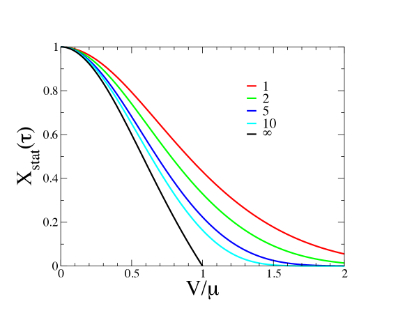
Figure 1: Plot of the asymptotic fluctuation-dissipation ratio $X_{\rm stat}(\tau)$ pertaining to the nonequilibrium stationary state on the chain in the low-temperature regime (see (LABEL:xlow)), against the ratio $V/\mu$, for $\mu^{2}\tau=1$, 2, 5, 10 and $\infty$ (the latter case corresponding to the asymptotic result (6.14)).

6.2 Arbitrary finite temperature

We now turn to the analysis of the nonequilibrium stationary state on the chain for an arbitrary finite temperature $T$.

The response function $R_{\rm stat}(\tau)$ falls off exponentially as $R_{\rm stat}(\tau)\sim{\rm e}^{-\alpha_{R}\tau}$, with

$$\alpha_{R}=2\left(1-\sqrt{1-V^{2}}\right)+\mu^{2}.$$ (6.20)

This asymptotic result can be derived in two ways: either by using the second line of (6.8) and the asymptotic growth $I_{0}(z)\sim{\rm e}^{z}$ of the modified Bessel function, or by evaluating the integral in the first line of (6.8) by the saddle-point method. The saddle-point equation reads $\tan q=-{\rm i}V$.

The asymptotic analysis of the correlation function $C_{\rm stat}(\tau)$ is more intricate. Consider the integral in the first line of (6.7). Its asymptotic behavior at large $\tau$ can be a priori governed by two special values of $q$: the saddle point at $q^{(I)}$ such that $\tan q^{(I)}=-{\rm i}V$, yielding the decay rate

$$\alpha^{(I)}=\alpha_{R}$$ (6.21)

(see (6.20)), and the zero of the denominator at $q^{(I\!I)}$ such that $\cos q^{(I\!I)}=1+\mu^{2}/2$, yielding the decay rate

$$\alpha^{(I\!I)}=V\mu\sqrt{\mu^{2}+4}=VT.$$ (6.22)

Both $q^{(I)}$ and $q^{(I\!I)}$ turn out to be purely imaginary. Hence the relevant decay rate is that pertaining to the special value of $q$ which is closer to the real axis, i.e., whose absolute imaginary part is the smaller. We have $q^{(I)}=q^{(I\!I)}$ (and so $\alpha^{(I)}=\alpha^{(I\!I)}$) at the borderline velocity

$$V_{c}=\frac{\mu\sqrt{\mu^{2}+4}}{\mu^{2}+2}=\frac{T}{\sqrt{T^{2}+4}}=\tanh{\hat{\mu}}.$$ (6.23)

The scenario put forward in the low-temperature scaling regime extends to the stationary state at any finite temperature.

• Regime I ($V<V_{c}$). In this regime, $q^{(I)}$ is closer to the real axis than $q^{(I\!I)}$, hence

  $$\alpha_{C}=\alpha_{R}=\alpha^{(I)}.$$ (6.24)

  The asymptotic fluctuation-dissipation ratio

  $$X_{\rm stat}(\infty)=\frac{2\left(1-1\left/\sqrt{1-V^{2}}\right.\right)+\mu^{2}}{2\left(1-\sqrt{1-V^{2}}\right)+\mu^{2}},$$ (6.25)

  i.e.,

  $$X_{{\rm stat}}(\infty)=\frac{1-\sqrt{1-V_{c}^{2}}\left/\sqrt{1-V^{2}}\right.}{1-\sqrt{1-V_{c}^{2}}\sqrt{1-V^{2}}},$$ (6.26)

  is consistently equal to the value of (5.5) at the saddle point ($q=q^{(I)}$). It decreases monotonically from unity to zero as $V$ is increased from 0 to $V_{c}$. Let us note that the expression (6.26) has exactly the same form as in the case of the Ising chain with asymmetric dynamics [11]. In the latter case, the relationship between $V_{c}$ and temperature is given by $V_{c}=\sqrt{1-\gamma^{2}}$, where $\gamma=\tanh 2/T$. As in (6.23), $V_{c}$ increases from $0$ to $1$, when $T$ varies between $0$ and infinity.

• Regime II ($V>V_{c}$). Now $q^{(I\!I)}$ is closer to the real axis than $q^{(I)}$, and so we have

  $$\alpha_{C}=\alpha^{(I\!I)}<\alpha_{R}=\alpha^{(I)}.$$ (6.27)

  The fluctuation-dissipation ratio falls off exponentially fast to zero, with a decay rate $\alpha^{(I)}-\alpha^{(I\!I)}$.

• Borderline situation ($V=V_{c}$). We have then

  $$\alpha_{C}=\alpha_{R}=\frac{2V_{c}^{2}}{\sqrt{1-V_{c}^{2}}}=\frac{\mu^{2}(\mu^{2}+4)}{\mu^{2}+2}=\frac{T^{2}}{\sqrt{T^{2}+4}}.$$ (6.28)

6.3 Spatial interpretation of the two regimes of fluctuation-dissipation violation

The existence of two regimes of fluctuation-dissipation violation, i.e., Regime I of weak violation, with a finite $X_{\rm stat}(\infty)$, and Regime II of strong violation, with a vanishing $X_{\rm stat}(\infty)$, has the following real-space interpretation. Let us start from the identity (5.3), which translates in real space into the convolution formula

$$C_{x,{\rm stat}}(\tau)=\sum_{y=-\infty}^{+\infty}C_{x-y,{\rm eq}}\,R_{y,{\rm stat}}(\tau).$$ (6.29)

The static correlation function $C_{x,{\rm eq}}$ is given by (6.3), while the space-dependent response function $R_{x,{\rm stat}}(\tau)$ reads

$$R_{x,{\rm stat}}(\tau) = {\rm e}^{-(2+\mu^{2})\tau}\int\frac{{\rm d}q}{2\pi}\,{\rm e}^{{\rm i}qx+2(\cos q-{\rm i}V\sin q)\tau}$$ (6.30)

$$= {\rm e}^{-(2+\mu^{2})\tau}\left(\frac{1+V}{1-V}\right)^{x/2}I_{x}\left(2\sqrt{1-V^{2}}\,\tau\right),$$

where $I_{x}$ is the modified Bessel function (see (3.19)). A very similar expression of the stationary response is found for the Ising chain under asymmetric dynamics [11]. Consider the expression (6.29) for the autocorrelation function ($x=0$), i.e.,

$$C_{\rm stat}(\tau)=\sum_{y=-\infty}^{+\infty}C_{-y,{\rm eq}}\,R_{y,{\rm stat}}(\tau).$$ (6.31)

The first factor falls off exponentially as $C_{-y,{\rm eq}}={\rm e}^{-{\hat{\mu}}|y|}$ (see (6.3)), where the decay rate ${\hat{\mu}}$ is the inverse equilibrium correlation length. The second factor, $R_{y,{\rm stat}}(\tau)$, exhibits, in the regime of long times, an exponential profile of the form

$$\frac{R_{y,{\rm stat}}(\tau)}{R_{0,{\rm stat}}(\tau)}\approx{\rm e}^{{\hat{\nu}}y},$$ (6.32)

characterized by the growth rate ${\hat{\nu}}$ or, equivalently, by the asymmetry length $\xi_{\rm asym}$:

$${\hat{\nu}}=\frac{1}{2}\ln\frac{1+V}{1-V}=\frac{1}{\xi_{\rm asym}}.$$ (6.33)

The two spatial rates ${\hat{\mu}}$ and ${\hat{\nu}}$, or, equivalently, the two lengths $\xi_{\rm eq}$ and $\xi_{\rm asym}$, coincide for $V=\tanh{\hat{\mu}}=V_{c}$ (see (6.23)).

In Regime I, i.e., for $V<V_{c}$, one has ${\hat{\nu}}<{\hat{\mu}}$ (i.e., $\xi_{\rm eq}<\xi_{\rm asym}$). The product $C_{-y,{\rm eq}}\,R_{y,{\rm stat}}(\tau)$ is therefore maximum at the origin ($y=0$), and so the sum over sites $y$ entering (6.31) is dominated by values of $y$ around the origin. We thus recover the result $\alpha_{C}=\alpha_{R}$ (see (6.24)).

In Regime II, i.e., for $V>V_{c}$, one has ${\hat{\nu}}>{\hat{\mu}}$ (i.e., $\xi_{\rm eq}>\xi_{\rm asym}$), and so the sum entering (6.31) is dominated by distant values of $y$. A more precise statement is as follows. The asymptotic behavior of the modified Bessel function

$$I_{n}(z)\sim\exp\left(\sqrt{n^{2}+z^{2}}-n\ln\frac{n+\sqrt{n^{2}+z^{2}}}{z}\right),$$ (6.34)

which holds whenever $n$ and $z$ are simultaneously large, translates into the asymptotic fall-off of the response function

$$R_{x,{\rm stat}}(\tau)\sim{\rm e}^{-\Psi(w)\,\tau}$$ (6.35)

in any direction of the $x$–$\tau$ plane such that $x=w\tau$, where

$$\Psi(w)=2 + \mu^{2}-\sqrt{w^{2}+4(1-V^{2})}$$ (6.36)

$$+ w\ln\frac{w+\sqrt{w^{2}+4(1-V^{2})}}{2(1+V)}.$$

The large-deviation function $\Psi(w)$ consistently obeys $\Psi(0)=\alpha_{R}$ (see (6.20)), as well as the symmetry property $\Psi(w)-\Psi(-w)=-2{\hat{\nu}}w$. It takes its minimum $\Psi=\mu^{2}$ for $w=2V$, so that the response function is maximum near the ballistic point $x=2V\tau$, where it falls off as ${\rm e}^{-\mu^{2}\tau}$. The asymptotic decay rate of the maximum response is thus identical to that of the local response for symmetric dynamics (see (6.20)).

Inserting the estimate (6.35) into (6.31), we are left with the expression

$$\alpha_{C}=\min_{w}\bigl{(}\Psi(w)-{\hat{\mu}}w\bigr{)},$$ (6.37)

where the minimum has to be attained for a positive value of $w$. We thus obtain

$$w=2(V\cosh{\hat{\mu}}-\sinh{\hat{\mu}}),\qquad\alpha_{C}=2V\sinh{\hat{\mu}}.$$ (6.38)

The first expression yields a positive solution ($w>0$) for $V>V_{c}=\tanh{\hat{\mu}}$, whereas the second expression is in agreement with (6.5), (6.22).

7 Nonequilibrium stationary state: higher dimension

We now turn to the analysis of specific features of the nonequilibrium stationary state in higher dimension.

The expressions (4.4) and (4.12) for the stationary correlation and response functions read explicitly

$$C_{\rm stat}(\tau) = \int\!{\frac{{\rm d}^{D}{\bf q}}{(2\pi)^{D}}}\frac{T}{\omega({\bf q})+\mu^{2}}\,{\rm e}^{-(\Omega({\bf q})+\mu^{2})\tau}$$

$$= T\!\int_{0}^{\infty}{\rm d}u\,{\rm e}^{-(2D+\mu^{2})(\tau+u)}\prod_{a=1}^{D}I_{0}\left(2\sqrt{(\tau+u)^{2}-V_{a}^{2}\tau^{2}}\right),$$

$$R_{\rm stat}(\tau) = \int\!{\frac{{\rm d}^{D}{\bf q}}{(2\pi)^{D}}}{\rm e}^{-(\Omega({\bf q})+\mu^{2})\tau}$$ (7.2)

$$= {\rm e}^{-(2D+\mu^{2})\tau}\prod_{a=1}^{D}I_{0}\left(2\sqrt{1-V_{a}^{2}}\,\tau\right),$$

where $I_{0}$ is the modified Bessel function (see (3.19)).

These expressions again demonstrate that the usual situation, where the correlation and response functions are positive and decay monotonically to zero, corresponds to the case where all the components of the velocity obey $|V_{a}|<1$. The asymptotic behavior of $C_{\rm stat}(\tau)$ and $R_{\rm stat}(\tau)$ can be studied along the lines of the one-dimensional case (see section 6). The asymptotic analysis of $C_{\rm stat}(\tau)$ again reveals the existence of two regimes.

• Regime I (${{\bf V}}$ small). In this regime, the decay of $C_{\rm stat}(\tau)$ and $R_{\rm stat}(\tau)$, as given by the integral representations in the first lines of (LABEL:chigh) and (7.2), is dominated by the same saddle point ${\bf q}^{(I)}$, defined by $\tan q^{(I)}_{a}=-{\rm i}V_{a}$. We have therefore

  $$\alpha_{C}=\alpha_{R}=\alpha^{(I)},$$ (7.3)

  with

  $$\alpha^{(I)}=2\sum_{a=1}^{D}\left(1-\sqrt{1-V_{a}^{2}}\right)+\mu^{2}.$$ (7.4)

  The asymptotic fluctuation-dissipation ratio is given by the value of (5.5) at the saddle point ${\bf q}^{(I)}$, i.e.,

  $$X_{\rm stat}(\infty)=\displaystyle{\displaystyle 2\sum_{a=1}^{D}\left(1-1\!\left/\!\sqrt{1-V_{a}^{2}}\right.\right)+\mu^{2}\over\displaystyle 2\sum_{a=1}^{D}\left(1-\sqrt{1-V_{a}^{2}}\right)+\mu^{2}}.$$ (7.5)

  This formula is a generalization of the one-dimensional result (6.25).

• Regime II (${{\bf V}}$ large). In this regime, the decay of $C_{\rm stat}(\tau)$ is obtained by constraining the saddle point to belong to the manifold with equation $\omega({\bf q})+\mu^{2}=0$. In other words, this decay is dominated by the wavevector ${\bf q}^{(I\!I)}$ so that $\Omega({\bf q}^{(I\!I)})$ is extremal while $\omega({\bf q}^{(I\!I)})+\mu^{2}$ vanishes. We have again

  $$\alpha_{C}=\alpha^{(I\!I)}<\alpha_{R}=\alpha^{(I)},$$ (7.6)

  and the fluctuation-dissipation ratio falls off exponentially fast.

  More explicitly, introducing a Lagrange multiplier $\ell$, we are led to extremalize the quantity

  $$Q({\bf q},\ell)=\Omega({\bf q})-\ell\omega({\bf q}).$$ (7.7)

  Introducing for convenience the parameter $L=1/(1-\ell)$, this amounts to extremalizing

  $$U({\bf q},L)=\sum_{a=1}^{D}(1-\cos q_{a}+{\rm i}LV_{a}\sin q_{a}).$$ (7.8)

  The stationarity equations read $\tan q^{(I\!I)}_{a}=-{\rm i}LV_{a}$. We thus obtain

  $$\alpha^{(I\!I)}=2L\sum_{a=1}^{D}\frac{V_{a}^{2}}{\sqrt{1-L^{2}V_{a}^{2}}},$$ (7.9)

  where the parameter $L$ obeys the consistency condition $\omega({\bf q}^{(I\!I)})+\mu^{2}=0$, i.e.,

  $$\mu^{2}=2\sum_{a=1}^{D}\left(\frac{1}{\sqrt{1-L^{2}V_{a}^{2}}}-1\right).$$ (7.10)

  Regime II holds as long as $L<1$, so that the imaginary parts of the $q_{a}^{(I\!I)}$ are smaller than those of the $q_{a}^{(I)}$.

• Borderline situation. The borderline situation between Regimes I and II corresponds to $L=1$. We thus have

  $$\mu^{2}=2\sum_{a=1}^{D}\left(\frac{1}{\sqrt{1-V_{a}^{2}}}-1\right).$$ (7.11)

  The numerator of the asymptotic fluctuation-dissipation ratio (7.5) consistently vanishes. At the borderline, we have

  $$\alpha_{C}=\alpha_{R}=\alpha^{(I)}=\alpha^{(I\!I)}=2\sum_{a=1}^{D}\frac{V_{a}^{2}}{\sqrt{1-V_{a}^{2}}}.$$ (7.12)

  This formula is a generalization of the one-dimensional result (6.28).

The borderline velocities obeying (7.11) run over a closed borderline surface $\SS$ in the $D$-dimensional space of velocities ${{\bf V}}$. Regime I (weak violation of the fluctuation-dissipation theorem), with its finite asymptotic fluctuation-dissipation ratio (7.5), holds for velocities inside the surface $\SS$, while Regime II (strong violation of the fluctuation-dissipation theorem) holds outside the surface $\SS$. The size of the borderline surface $\SS$ increases with $\mu$, i.e., with the distance to the critical point.

• For $\mu$ small, i.e., $T$ just above $T_{c}$, isotropy in velocity space is restored, since ${{\bf V}}$ is only involved through its norm $|{{\bf V}}|$. In Regime I, (7.4) and (7.5) indeed respectively become

  $$\alpha^{(I)}\approx\mu^{2}+{{\bf V}}^{2}$$ (7.13)

  and

  $$X_{\rm stat}(\infty)\approx\frac{\mu^{2}-{{\bf V}}^{2}}{\mu^{2}+{{\bf V}}^{2}}.$$ (7.14)

  The surface $\SS$ is thus a small sphere of radius $\mu$. In Regime II, (7.9) and (7.10) yield

  $$L=\frac{\mu}{|{{\bf V}}|}$$ (7.15)

  and

  $$\alpha^{(I\!I)}=2\mu|{{\bf V}}|.$$ (7.16)

• In the opposite limit ($\mu$ large, i.e., $T$ large), the surface $\SS$ approaches the unit cube from inside.

Figure 2 shows a plot of the borderline curve $\SS$ for the square lattice in the $V_{1}$–$V_{2}$ plane, with equation

$$\frac{1}{\sqrt{1-V_{1}^{2}}}+\frac{1}{\sqrt{1-V_{2}^{2}}}=2+\frac{\mu^{2}}{2}$$ (7.17)

(see (7.11)), for the values of $\mu$ given in table 2, together with the corresponding temperatures.

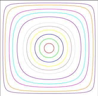
Figure 2: Plot of the borderline curve $\SS$ for the square lattice in the $V_{1}$–$V_{2}$ plane, for the values of $\mu$ listed in table 2. The outermost square is the unit square.

$\mu$	0.1	0.2	0.3	0.4	0.5	0.6	0.8	1	1.2	1.6	2
$T$	1.559	1.888	2.159	2.410	2.654	2.897	3.399	3.936	4.521	5.860	7.454

Table 2: List of the values of the parameter $\mu$ for which the borderline curve $\SS$ for the square lattice in shown in figure 2, together with the corresponding values of temperature $T$ (see (3.36)).

8 Low-temperature scaling regime in one dimension

This section and the three following ones are devoted to the transient regime of the model, before the nonequilibrium stationary state sets in. The duration of this regime is measured by the relaxation time $\tau_{\rm eq}=1/(2\mu^{2})$ (see (3.30)). The latter is finite in the paramagnetic phase ($T>T_{c}$), whereas the transient regime lasts forever (the system is aging) both at the critical point ($T=T_{c}$) and in the whole low-temperature ferromagnetic phase ($T<T_{c}$).

In this section we consider the scaling behavior of the one-dimensional model at low temperature, in the regime where $\mu$ and $V$ are small, whereas times $s$ and $t$ are large. The critical regime in higher dimension will be analyzed in sections 9 and 10 for $D>4$ and $2<D<4$ respectively. Finally, the dynamics in the low-temperature ferromagnetic phase ($T<T_{c}$) will be the subject of section 11.

8.1 One-time observables

Let us start the analysis with the functions $f(t)$ and $g(t)$. In the scaling regime, (3.20) and (3.22) (or (3.32)) yield

$$f^{\rm L}(p)\approx\frac{1}{\sqrt{8p}},\qquad g^{\rm L}(p)\approx\frac{1}{\sqrt{8p}-4\mu},$$ (8.1)

hence

$$f(t)\approx\frac{1}{\sqrt{8\pi t}},\qquad g(t)\approx\frac{1}{\sqrt{8\pi t}}+\frac{\mu}{2}\,{\rm e}^{2\mu^{2}t}\bigl{(}1+\mathop{\rm erf}\nolimits(\mu\sqrt{2t})\bigr{)}.$$ (8.2)

A quantity of interest in this regime is the reduced dynamical susceptibility

$$\chi(t)=\sum_{x=-\infty}^{+\infty}C_{x}(t)=C^{\rm F}(0,t)=\frac{1}{g(t)}\left(1+4\mu\int_{0}^{t}{\rm d}s\,g(s)\right).$$ (8.3)

This quantity provides a measure of the range of the correlations, i.e., of the typical size of the ordered domains at time $t$. Using (8.2) and working out the integral in (8.3), (or alternatively using (8.7) below) we can recast the dynamical susceptibility into the scaling form

$$\chi(t)\approx\chi_{\rm stat}\,F(x),$$ (8.4)

where $\chi_{\rm stat}\approx{2}/{\mu}$ is the static susceptibility, and $F(x)$ is the scaling function

$$F(x)=\frac{{\rm e}^{x^{2}}(1+\mathop{\rm erf}\nolimits x)}{\frac{1}{x\sqrt{\pi}}+{\rm e}^{x^{2}}(1+\mathop{\rm erf}\nolimits x)},$$ (8.5)

with $x=\mu\sqrt{2t}=\sqrt{t/\tau_{\rm eq}}$. The scaling law (8.4) interpolates between the coarsening regime ($t\ll\tau_{\rm eq}$) and the stationary regime ($t\gg\tau_{\rm eq}$). In the first case, i.e., for $x\ll 1$, the square-root behavior $F(x)\approx x\sqrt{\pi}$ yields the coarsening law

$$\chi(t)\approx\sqrt{8\pi t}.$$ (8.6)

In the second case, i.e., for $x\gg 1$, the behavior $F(x)\approx 1-2{\rm e}^{-x^{2}}/(x\sqrt{\pi})$ yields an exponential convergence of the dynamical susceptibility to its static value $\chi_{\rm stat}$.

To close, let us mention that the full structure factor $C^{\rm F}(q,t)$ can be derived explicitly in the scaling regime. Starting from (3.13) and using again (8.2), we get

$$C^{\rm F}(q,t) \approx \frac{{\rm e}^{-2q^{2}t}}{g(t)}\left(1+4\mu\int_{0}^{t}{\rm d}s\,{\rm e}^{2q^{2}s}g(s)\right)$$ (8.7)

$$\approx \frac{\mu^{2}\,{\rm e}^{2\mu^{2}t}\bigl{(}1\!+\!\mathop{\rm erf}\nolimits(\mu\sqrt{2t})\bigr{)}+q\,{\rm e}^{-2q^{2}t}\bigl{(}q-{\rm i}\mu\mathop{\rm erf}\nolimits({\rm i}q\sqrt{2t})\bigr{)}}{(q^{2}+\mu^{2})g(t)}.$$

This expression interpolates continuously between the Gaussian line-shape

$$C^{\rm F}(q,t)\approx\sqrt{8\pi t}\,{\rm e}^{-2q^{2}t}$$ (8.8)

in the coarsening regime and the Lorentzian one

$$C_{\rm eq}^{\rm F}(q)\approx\frac{2\mu}{q^{2}+\mu^{2}}$$ (8.9)

in the stationary state.

8.2 Two-time observables

Let us now analyze the two-time correlation and response functions $C(t,s)$ and $R(t,s)$ and the corresponding fluctuation-dissipation ratio $X(t,s)$ in the scaling regime. Starting from (3.13), (4.3) and (4.10), and performing the Gaussian integrals over $q$, we obtain

$$C(t,s) \approx \frac{1}{\sqrt{g(t)g(s)}}$$

$$\times \left(\frac{{\rm e}^{-V^{2}(t-s)^{2}/(t+s)}}{\sqrt{4\pi(t+s)}}+4\mu\int_{0}^{s}{\rm d}u\,\frac{{\rm e}^{-V^{2}(t-s)^{2}/(t+s-2u)}}{\sqrt{4\pi(t+s-2u)}}g(u)\right),$$

$$R(t,s) \approx \frac{{\rm e}^{-V^{2}(t-s)}}{\sqrt{4\pi(t-s)}}\sqrt{\frac{g(s)}{g(t)}},$$ (8.10)

where the function $g(t)$ is given in (8.2). Many different sub-cases can be analyzed from the general expressions (8.10), according to the values of the dimensionless combinations $\mu^{2}s$, $\mu^{2}t$, $V^{2}s$ and $V^{2}t$. The most interesting of these regimes are as follows.

Stationary regime.

This regime is reached when the waiting time $s$ is much larger than $\tau_{\rm eq}$ ($\mu^{2}s\gg 1$). The function $g(t)$ obeys the exponential growth (3.29). The corresponding two-time quantities have been studied in section 6.1.

Coarsening regime.

This regime corresponds to the zero-temperature limit of the reversible dynamics ($\mu=V=0$). The resulting scale-invariant coarsening dynamics has been investigated earlier [15]. The expressions (8.10) simplify to

$$C(t,s) \approx \left(\frac{4ts}{(t+s)^{2}}\right)^{1/4},$$

$$R(t,s) \approx \frac{1}{\sqrt{4\pi(t-s)}}\left(\frac{t}{s}\right)^{1/4}.$$ (8.11)

The corresponding fluctuation-dissipation ratio reads

$$X(t,s)\approx T\left(\frac{2s}{\pi}\right)^{1/2}\left(\frac{t+s}{t-s}\right)^{3/2},$$ (8.12)

and especially (see (4.17))

$$X_{\rm as}(s)\approx T\left(\frac{2s}{\pi}\right)^{1/2}.$$ (8.13)

Anomalous aging.

This regime corresponds to the zero-temperature limit of the irreversible dynamics ($\mu=0$, while $V\neq 0$). The expressions (8.10) simplify to

$$C(t,s) \approx \left(\frac{4ts}{(t+s)^{2}}\right)^{1/4}{\rm e}^{-V^{2}(t-s)^{2}/(t+s)},$$

$$R(t,s) \approx \frac{{\rm e}^{-V^{2}(t-s)}}{\sqrt{4\pi(t-s)}}\left(\frac{t}{s}\right)^{1/4}.$$ (8.14)

The response function $R(t,s)$ exhibits an exponential decay in $\tau=t-s$, characterized by the microscopic time scale $1/V^{2}$. The correlation function $C(t,s)$ however exhibits a richer behavior in the late-time regime ($V^{2}s\gg 1$), with an intermediate anomalous aging regime [34] for $\tau\ll s$, where it assumes the Gaussian form

$$C(t,s)\approx{\rm e}^{-V^{2}\tau^{2}/(2s)},$$ (8.15)

which falls over a characteristic time growing as $\sqrt{s}/V$. When $\tau$ becomes of the order of the waiting time $s$, the correlation function is already exponentially small in the variable $V^{2}s$. Its subsequent decay to zero follows an exponential law, characterized by the same microscopic time scale $1/V^{2}$ as the response function. The same regime can be observed in the case of the Ising chain with asymmetric dynamics [11].

Asymptotic regime.

This regime corresponds to the limit of a very long time difference $\tau=t-s$, while the combinations $\mu^{2}s$ and $V^{2}s$ remain finite. It is the non-stationary counterpart of the large-$\tau$ stationary regime investigated in section 6. Here again, rather than using the expressions (8.10), it is advantageous to return to the integral expressions (4.4) and (4.12). For large $\tau$, the latter integrals are dominated by a saddle point at $q^{(I)}=-{\rm i}V$. We thus obtain the following estimates:

$$C(t,s) \approx \frac{{\rm e}^{-(\mu^{2}+V^{2})\tau}}{\sqrt{4\pi\tau}}\,{\rm e}^{-\mu^{2}s}\sqrt{\frac{g(s)}{\mu}}\,C^{\rm F}(-{\rm i}V,s),$$

$$R(t,s) \approx \frac{{\rm e}^{-(\mu^{2}+V^{2})\tau}}{\sqrt{4\pi\tau}}\,{\rm e}^{-\mu^{2}s}\sqrt{\frac{g(s)}{\mu}}.$$ (8.16)

The structure factor $C^{\rm F}(-{\rm i}V,s)$ entering the first of these expressions is given by the analytic continuation of (8.7).

One of the most physically relevant quantities characterizing the transient regime, before the stationary state sets in, is the asymptotic fluctuation-dissipation ratio $X_{\rm as}(s)$ (see (4.17)). Defining the scaling variables $x$ and $y$ by

$$x=\mu\sqrt{2s},\qquad y=V\!\sqrt{2s},$$ (8.17)

the expressions (8.16), together with (8.2) and (8.7), yield the scaling formula

$$\frac{1}{X_{\rm as}(s)}\approx 2+\frac{N(x,y)}{2x(x^{2}-y^{2})\left(\frac{1}{\sqrt{\pi}}+x\,{\rm e}^{x^{2}}(1+\mathop{\rm erf}\nolimits x)\right)^{2}},$$ (8.18)

with

$$N(x,y) = \left(\frac{1+2(3y^{2}-x^{2})}{\sqrt{\pi}}+2x(3y^{2}-x^{2})\,{\rm e}^{x^{2}}(1+\mathop{\rm erf}\nolimits x)\right)$$ (8.19)

$$\times \left(x^{2}\,{\rm e}^{x^{2}}(1+\mathop{\rm erf}\nolimits x)-y\,{\rm e}^{y^{2}}(y+x\mathop{\rm erf}\nolimits y)\right).$$

In the borderline situation where $x=y$, i.e., $V=V_{c}=\mu$, the above expression simplifies to

$$\frac{1}{X_{\rm as}(s)}\approx 2+\frac{N_{0}(x)}{4x\left(\frac{1}{\sqrt{\pi}}+x\,{\rm e}^{x^{2}}(1+\mathop{\rm erf}\nolimits x)\right)^{2}},$$ (8.20)

with

$$N_{0}(x) = \left(\frac{1+4x^{2}}{\sqrt{\pi}}+4x^{3}\,{\rm e}^{x^{2}}(1+\mathop{\rm erf}\nolimits x)\right)$$ (8.21)

$$\times \left(\frac{2x}{\sqrt{\pi}}+2(x^{2}+1)\,{\rm e}^{x^{2}}+(2x^{2}+1)\,{\rm e}^{x^{2}}\mathop{\rm erf}\nolimits x\right).$$

At the coarsening end, i.e., when $x$ and $y$ are small, the fluctuation-dissipation ratio has the series expansion

$$X_{\rm as}(s) \approx \frac{2}{\sqrt{\pi}}\,x+\frac{4(\pi-3)}{\pi}\,x^{2}+\frac{2(\pi-3)(\pi-12)}{\pi^{3/2}}\,x^{3}$$ (8.22)

$$- \frac{14}{\sqrt{\pi}}\,xy^{2}+\cdots$$

The first term agrees with (8.13), whereas only the last one shows a dependence on $V$.

At the stationary end, i.e., when $x$ and $y$ are large, the distinction between the stationary Regimes I and II shows up as follows.

• For $y<x$, i.e., $V<\mu$, we have

  $$X_{\rm as}(s)\approx\frac{x^{2}-y^{2}}{x^{2}+y^{2}}\left(1+\frac{y(x+y)(3y^{2}-x^{2})}{2x^{2}(x^{2}+y^{2})}\,{\rm e}^{-(x^{2}-y^{2})}\right).$$ (8.23)

  The limit value of this expression is in agreement with the stationary ratio $X_{\rm stat}(\infty)$ in Regime I, given by (6.14). In other words, we have

  $$\lim_{s\to\infty}X_{\rm as}(s)=\lim_{\tau\to\infty}X_{\rm stat}(\tau).$$ (8.24)

  This identity testifies that the convergence of the fluctuation-dissipation ratio to the value $X_{\rm stat}(\infty)$ is uniform in the $s$–$t$ plane, irrespective of the direction, provided both times $s$ and $t$ are much larger than $\tau_{\rm eq}$ and $1/V^{2}$.

  The fluctuation-dissipation ratio $X_{\rm as}(s)$ increases monotonically and reaches its limit from below for $y/x<1/\sqrt{3}$, i.e., $1/2<X_{\rm as}(\infty)<1$, whereas it exhibits a maximum and reaches its limit from above for $1/\sqrt{3}<y/x<1$, i.e., $X_{\rm as}(\infty)<1/2$. This feature will also hold in higher dimension, where the value $X_{\rm as}(\infty)=1/2$ will always be singled out.

• For $y>x$, i.e., $V>\mu$, the fluctuation-dissipation ratio falls off exponentially as

  $$X_{\rm as}(s)\approx\frac{2x^{2}(y-x)}{y(x+y)(3y^{2}-x^{2})}\,{\rm e}^{-(y^{2}-x^{2})}.$$ (8.25)

  This corresponds to the stationary Regime II.

• In the borderline situation where $x=y$, i.e., $V=V_{c}=\mu$, the fluctuation-dissipation ratio, given by (8.20), falls off as a power law:

  $$X_{\rm as}(s)\approx\frac{1}{2x^{2}}\approx\frac{1}{4\mu^{2}s}.$$ (8.26)

Figure 3 shows a plot of the asymptotic fluctuation-dissipation ratio $X_{\rm as}(s)$ against the scaling variable $x=\mu\sqrt{2s}$, for several values of the ratio $y/x=V/\mu$.

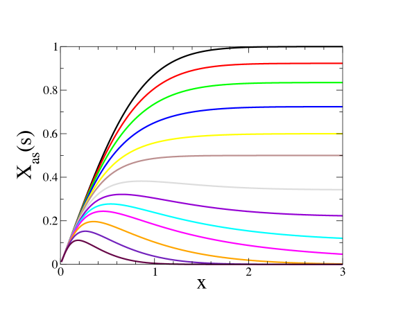
Figure 3: Plot of the asymptotic fluctuation-dissipation ratio $X_{\rm as}(s)$ in the low-temperature scaling regime in one dimension (see (8.18)) against the scaling variable $x=\mu\sqrt{2s}$, for the following values of the ratio $V/\mu$ (top to bottom): 0 (reversible), 0.2, 0.3, 0.4, 0.5, $1/\sqrt{3}\approx 0.577350$ (so that $X_{\rm stat}(\infty)=1/2$), 0.7, 0.8, 0.9, 1 (borderline case), 1.2, 1.5 and 2.

9 Classical critical regime ($D>4$)

In this section we study the transient properties of the model in the vicinity of its critical temperature for $D>4$, where the critical exponent $\nu=1/2$ assumes its mean-field or ‘classical’ value. We assume that $\mu$ and ${{\bf V}}$ are small, whereas times $s$ and $t$ are large. The dynamical properties of the model obey scaling laws throughout the scaling regime thus defined.

9.1 One-time observables

The constants $A_{1}$ and $A_{2}$ defined in (3.24) are finite. As a consequence, (3.20) and (3.23) yield in the scaling regime

$$g^{\rm L}(p)\approx\frac{G}{p-2\mu^{2}},\qquad G=\frac{A_{1}^{2}}{A_{2}},$$ (9.1)

hence

$$g(t)\approx G\,{\rm e}^{2\mu^{2}t}.$$ (9.2)

The structure factor $C^{\rm F}({\bf q},t)$ can be derived explicitly in the scaling regime. Keeping only the integral term in (3.13) and using (9.2), we get

$$C^{\rm F}({\bf q},t)\approx T_{c}\,\frac{1-{\rm e}^{-2({\bf q}^{2}+\mu^{2})t}}{{\bf q}^{2}+\mu^{2}}.$$ (9.3)

The reduced dynamical susceptibility $\chi(t)=C^{\rm F}({\bf 0},t)$ therefore reads

$$\chi(t)\approx T_{c}\,\frac{1-{\rm e}^{-2\mu^{2}t}}{\mu^{2}}.$$ (9.4)

This quantity exhibits a linear growth $\chi(t)\approx 2T_{c}t$ in the coarsening regime, and saturates to the static value $\chi_{\rm stat}=T_{c}/\mu^{2}$ in the stationary state.

9.2 Two-time observables

In order to study the two-time correlation and response functions, we again start from (3.13), (4.3) and (4.10), use (9.2), and perform the Gaussian integrals over ${\bf q}$. We thus obtain

$$C(t,s) \approx 2T_{c}\,{\rm e}^{-\mu^{2}(t-s)}\int_{0}^{s}{\rm d}u\,\frac{{\rm e}^{-2\mu^{2}(s-u)-{{\bf V}}^{2}(t-s)^{2}/(t+s-2u)}}{(4\pi(t+s-2u))^{D/2}},$$

$$R(t,s) \approx \frac{{\rm e}^{-(\mu^{2}+{{\bf V}}^{2})(t-s)}}{(4\pi(t-s))^{D/2}}.$$ (9.5)

The response function does not exhibit any aging property: it coincides with the continuum limit of its stationary expression (7.2). Many different sub-cases follow from the general expressions (9.5). We again restrict the study to the most interesting ones.

Critical coarsening.

This scale-invariant regime corresponds to the reversible dynamics at the critical point ($\mu=0$, ${{\bf V}}={\bf 0}$) [15]. The expressions (9.5) simplify to

$$C(t,s) \approx \frac{2T_{c}}{(D-2)(4\pi)^{D/2}}\left((t-s)^{-(D-2)/2}-(t+s)^{-(D-2)/2}\right),$$

$$R(t,s) \approx \frac{1}{(4\pi(t-s))^{D/2}}.$$ (9.6)

The corresponding fluctuation-dissipation ratio,

$$X(t,s)\approx\frac{1}{1+\left(\displaystyle{\displaystyle t-s\over\displaystyle t+s}\right)^{D/2}},$$ (9.7)

only depends on the ratio $t/s$. In the limit where this time ratio is very large, the fluctuation-dissipation ratio tends to a finite value

$$X_{\infty}=\lim_{s\to\infty}\lim_{\tau\to\infty}X(t,s)=\frac{1}{2},$$ (9.8)

which has been emphasized [3, 15] to be a new universal amplitude ratio pertaining to nonequilibrium critical dynamics.

Anomalous aging.

This regime corresponds to the irreversible dynamics at the critical point ($\mu=0$, while ${{\bf V}}\neq{\bf 0}$). As in one dimension, the two-point correlation function exhibits an intermediate anomalous aging regime for $\tau\ll s$. The scaling form of $C(t,s)$ is however more complex than the Gaussian form (8.15). A scaling analysis of the integral entering (9.5), neglecting $\tau$ with respect to $s$ and integrating over $z=s/u$, indeed yields

$$C(t,s) \approx \frac{2T_{c}}{(8\pi)^{D/2}s^{(D-2)/2}}\int_{1}^{\infty}{\rm d}z\,{\rm e}^{-{{\bf V}}^{2}\tau^{2}z/(2s)}z^{(D-4)/2}$$ (9.9)

$$\approx \frac{T_{c}}{(4\pi)^{D/2}(|{{\bf V}}|\tau)^{D-2}}\;\Gamma\left(\frac{D-2}{2},\frac{{{\bf V}}^{2}\tau^{2}}{2s}\right),$$

where

$$\Gamma(a,x)=\int_{x}^{\infty}{\rm d}y\,{\rm e}^{-y}y^{a-1}$$ (9.10)

is the complementary incomplete Gamma function.

Asymptotic regime.

This asymptotic regime is the non-stationary counterpart of the large-$\tau$ stationary regime of section 7. The two-time response function (9.5) is already in asymptotic form, whereas for large $\tau$ the integral expression (4.4) for the two-time correlation function is dominated by a saddle point at ${\bf q}^{(I)}=-{\rm i}{{\bf V}}$. Using (9.2) and (9.3), we obtain

$$C(t,s)\approx T_{c}\frac{{\rm e}^{-(\mu^{2}+{{\bf V}}^{2})\tau}}{(4\pi\tau)^{D/2}}\,\frac{1-{\rm e}^{-2(\mu^{2}-{{\bf V}}^{2})s}}{\mu^{2}-{{\bf V}}^{2}}.$$ (9.11)

The asymptotic fluctuation-dissipation ratio $X_{\rm as}(s)$ is therefore

$$X_{\rm as}(s)\approx\frac{\mu^{2}-{{\bf V}}^{2}}{\mu^{2}+{{\bf V}}^{2}+(\mu^{2}-3{{\bf V}}^{2})\,{\rm e}^{-2(\mu^{2}-{{\bf V}}^{2})s}}.$$ (9.12)

Introducing the the scaling variables

$$x=\mu\sqrt{2s},\qquad y=|{{\bf V}}|\sqrt{2s},$$ (9.13)

(see (8.17)), the above result reads

$$X_{\rm as}(s)\approx\frac{x^{2}-y^{2}}{x^{2}+y^{2}+(x^{2}-3y^{2})\,{\rm e}^{-(x^{2}-y^{2})}}.$$ (9.14)

At the critical end, i.e., when $\mu^{2}s$ and ${{\bf V}}^{2}s$ are small, the fluctuation-dissipation ratio has the series expansion

$$X_{\rm as}(s)\approx\frac{1}{2}\left(1+(\mu^{2}-3{{\bf V}}^{2})\,s+\cdots\right),$$ (9.15)

whose first term agrees with (9.8).

At the stationary end, the distinction between the stationary Regimes I and II shows up as follows.

• For ${{\bf V}}^{2}<\mu^{2}$, we have

  $$X_{\rm as}(s)\approx\frac{\mu^{2}-{{\bf V}}^{2}}{\mu^{2}+{{\bf V}}^{2}}\left(1+\frac{3{{\bf V}}^{2}-\mu^{2}}{\mu^{2}+{{\bf V}}^{2}}\,{\rm e}^{-2(\mu^{2}-{{\bf V}}^{2})s}\right).$$ (9.16)

  The limit value is in agreement with the stationary $X_{\rm stat}(\infty)$ (see (7.14)) in Regime I. The fluctuation-dissipation ratio increases monotonically and reaches its limit from below for ${{\bf V}}^{2}<\mu^{2}/3$, i.e., $1/2<X_{\rm stat}(\infty)<1$, whereas it decreases monotonically and reaches its limit from above for ${{\bf V}}^{2}>\mu^{2}/3$, i.e., $X_{\rm stat}(\infty)<1/2$. In the special case where ${{\bf V}}^{2}=\mu^{2}/3$, i.e., $y=x/\sqrt{3}$, we have $X_{\rm as}(s)=1/2$ for all values of $s$.

• For ${{\bf V}}^{2}>\mu^{2}$, the fluctuation-dissipation ratio falls off exponentially as

  $$X_{\rm as}(s)\approx\frac{{{\bf V}}^{2}-\mu^{2}}{3{{\bf V}}^{2}-\mu^{2}}\,{\rm e}^{-2({{\bf V}}^{2}-\mu^{2})s}.$$ (9.17)

  This corresponds to the stationary Regime II.

• In the borderline situation where ${{\bf V}}^{2}=\mu^{2}$, the fluctuation-dissipation ratio again falls off as

  $$X_{\rm as}(s)\approx\frac{1}{2x^{2}}\approx\frac{1}{4\mu^{2}s}.$$ (9.18)

Figure 4 shows a plot of the asymptotic fluctuation-dissipation ratio $X_{\rm as}(s)$ against $x^{2}=2\mu^{2}s$, for several values of the ratio $|{{\bf V}}|/\mu$.

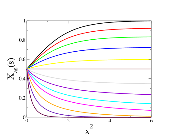
Figure 4: Plot of the asymptotic fluctuation-dissipation ratio $X_{\rm as}(s)$ in the classical critical regime ($D>4$) (see (9.12)) against $x^{2}=2\mu^{2}s$, for the following values of the ratio $|{{\bf V}}|/\mu$ (top to bottom): 0 (reversible), 0.2, 0.3, 0.4, 0.5, $1/\sqrt{3}\approx 0.577350$ (so that $X_{\rm as}(s)=1/2$ for all $s$), 0.7, 0.8, 0.9, 1 (borderline case), 1.2, 1.5 and 2.

10 Non-classical critical regime ($2<D<4$)

In this section we study the transient properties of the model in the vicinity of its critical temperature for $2<D<4$, where the critical exponent $\nu=1/(D-2)$ depends continuously on dimension. We again assume that $\mu$ and ${{\bf V}}$ are small, whereas times $s$ and $t$ are large.

10.1 One-time observables

Let us, for convenience, parametrize dimension as

$$D=2(1+\varepsilon)\qquad(0<\varepsilon<1),$$ (10.1)

so that $\nu=1/(2\varepsilon)$. In the scaling regime, (3.20) and (3.23) yield

$$f^{\rm L}(p)\approx A_{1}-Cp^{\varepsilon},\qquad g^{\rm L}(p)\approx\frac{G}{p^{\varepsilon}-(2\mu^{2})^{\varepsilon}},$$ (10.2)

with

$$C=(8\pi)^{-1-\varepsilon}|\Gamma(-\varepsilon)|,\qquad G=\frac{A_{1}^{2}}{C}.$$ (10.3)

We have therefore

$$g(t)\approx\frac{G}{\varepsilon}(2\mu^{2})^{1-\varepsilon}\,h_{\varepsilon}(2\mu^{2}t),$$ (10.4)

where the scaling function $h_{\varepsilon}$ reads

$$h_{\varepsilon}(\xi)=\int_{{\cal C}_{1}}\frac{{\rm d}z}{2\pi{\rm i}}\,\frac{\varepsilon}{z^{\varepsilon}-1}\,{\rm e}^{z\xi}={\rm e}^{\xi}+\int_{{\cal C}_{0}}\frac{{\rm d}z}{2\pi{\rm i}}\,\frac{\varepsilon}{z^{\varepsilon}-1}\,{\rm e}^{z\xi}.$$ (10.5)

By folding the contour ${\cal C}_{0}$ around the cut (i.e., $z\to-\rho\pm{\rm i}0$), we obtain the integral representation

$$h_{\varepsilon}(\xi)={\rm e}^{\xi}+\frac{\varepsilon\,\sin\pi\varepsilon}{\pi}\int_{0}^{\infty}{\rm d}\rho\,\frac{{\rm e}^{-\rho\xi}}{\rho^{\varepsilon}+\rho^{-\varepsilon}-2\cos\pi\varepsilon}.$$ (10.6)

Finally, the series expansion

$$h_{\varepsilon}(\xi)=\varepsilon\sum_{n\geq 1}\frac{\xi^{n\varepsilon-1}}{\Gamma(n\varepsilon)}=\varepsilon\frac{{\rm d}}{{\rm d}\xi}E_{\varepsilon}(\xi^{\varepsilon})$$ (10.7)

relates $h_{\varepsilon}$ to the Mittag-Leffler function $E_{\varepsilon}$.

In the coarsening regime, corresponding to small values of the scaling variable $\xi$, the scaling function $h_{\varepsilon}$ diverges as a power law:

$$h_{\varepsilon}(\xi)\approx\frac{\varepsilon}{\Gamma(\varepsilon)}\,\xi^{\varepsilon-1}.$$ (10.8)

At the stationary end, corresponding to large values of $\xi$, it grows exponentially as

$$h_{\varepsilon}(\xi)\approx{\rm e}^{\xi}.$$ (10.9)

The behavior of the reduced dynamical susceptibility $\chi(t)=C^{\rm F}({\bf 0},t)$ in the scaling regime can be estimated by keeping only the integral term in (3.13) and using (10.4). We thus obtain

$$\chi(t)\approx\frac{2T_{c}}{h_{\varepsilon}(2\mu^{2}t)}\int_{0}^{t}{\rm d}s\,h_{\varepsilon}(2\mu^{2}s).$$ (10.10)

In the coarsening regime (see (10.8)), the susceptibility exhibits the linear growth $\chi(t)\approx(2T_{c}t)/\varepsilon$. At the stationary end (see (10.9)), the susceptibility saturates to its static value $\chi_{\rm stat}=T_{c}/\mu^{2}$.

The following special values of $\varepsilon$ are of interest, as they correspond to integer dimensions. We shall return to them at the end of section 10.2.

• $D=2$ (i.e., $\varepsilon=0$). This case corresponds to the lower critical dimension of the model. We have

  $$h_{0}(\xi)=\int_{0}^{\infty}{\rm d}x\,\frac{\xi^{x-1}}{\Gamma(x)}={\rm e}^{\xi}+\int_{0}^{\infty}{\rm d}\rho\,\frac{{\rm e}^{-\rho\xi}}{(\ln\rho)^{2}+\pi^{2}}.$$ (10.11)

  The equality between the two integral expressions is attributed to Ramanujan [35].

• $D=3$ (i.e., $\varepsilon=1/2$). This case is the only non-trivial one with integer dimension. The scaling function reads

  $$h_{1/2}(\xi)=\frac{1}{\sqrt{4\pi\xi}}+\frac{1}{2}{\rm e}^{\xi}(1+\mathop{\rm erf}\nolimits\!\sqrt{\xi}).$$ (10.12)

• $D=4$ (i.e., $\varepsilon=1$). This case corresponds to the upper critical dimension of the model. The scaling function becomes a simple exponential:

  $$h_{1}(\xi)={\rm e}^{\xi}$$ (10.13)

  (see the comment at the very end of section 10.2).

10.2 Two-time observables

Starting from (3.13), (4.3) and (4.10) and performing the Gaussian integrals over ${\bf q}$, we are left with the following expressions for the two-time correlation and response functions in the scaling regime:

$$C(t,s) \approx \frac{2T_{c}}{\sqrt{h_{\varepsilon}(2\mu^{2}t)h_{\varepsilon}(2\mu^{2}s)}}\int_{0}^{s}{\rm d}u\,\frac{{\rm e}^{-{{\bf V}}^{2}(t-s)^{2}/(t+s-2u)}}{(4\pi(t+s-2u))^{D/2}}\,h_{\varepsilon}(2\mu^{2}u),$$

$$R(t,s) \approx \frac{{\rm e}^{-{{\bf V}}^{2}(t-s)}}{(4\pi(t-s))^{D/2}}\sqrt{\frac{h_{\varepsilon}(2\mu^{2}s)}{h_{\varepsilon}(2\mu^{2}t)}}.$$ (10.14)

In what follows we restrict the study to the most interesting of the different sub-cases which can be investigated from these general expressions, according to the values of the dimensionless combinations $\mu^{2}s$, $\mu^{2}t$, ${{\bf V}}^{2}s$ and ${{\bf V}}^{2}t$.

Critical coarsening.

This scale-invariant regime corresponds to the reversible dynamics at the critical point ($\mu=0$, ${{\bf V}}={\bf 0}$) [15]. Owing to (10.8), the expressions (10.14) simplify to

$$C(t,s) \approx \frac{4T_{c}}{(D-2)(4\pi)^{D/2}(t-s)^{(D-2)/2}}\frac{t}{t+s}\left(\frac{t}{s}\right)^{-D/4},$$

$$R(t,s) \approx \frac{1}{(4\pi(t-s))^{D/2}}\left(\frac{t}{s}\right)^{1-D/4}.$$ (10.15)

The corresponding fluctuation-dissipation ratio reads

$$X(t,s)\approx\frac{1}{1+\displaystyle{\displaystyle 2\over\displaystyle D-2}\left(\displaystyle{\displaystyle t-s\over\displaystyle t+s}\right)^{2}}.$$ (10.16)

The asymptotic fluctuation-dissipation ratio assumes the universal value [15]

$$X_{\infty}=\frac{D-2}{D}.$$ (10.17)

Anomalous aging.

This regime corresponds to the irreversible dynamics at the critical point ($\mu=0$, while ${{\bf V}}\neq{\bf 0}$). The two-point correlation function again exhibits an intermediate anomalous aging regime for $\tau\ll s$. A scaling analysis of the integral entering (10.14), neglecting $\tau$ with respect to $s$ and integrating over the dimensionless variable $z=s/u$, yields

$$C(t,s)\approx\frac{T_{c}\,\Gamma((D-2)/2)}{(4\pi)^{D/2}(|{{\bf V}}|\tau)^{D-2}}\,{\rm e}^{-{{\bf V}}^{2}\tau^{2}/(2s)}.$$ (10.18)

Asymptotic regime.

The asymptotic regime is the non-stationary counterpart of the large-$\tau$ stationary regime analyzed in section 7. For large $\tau$, the integral expressions (4.4) and (4.12) are dominated by a saddle point at ${\bf q}^{(I)}=-{\rm i}{{\bf V}}$. We thus obtain the following estimates:

$$C(t,s) \approx \frac{{\rm e}^{-(\mu^{2}+{{\bf V}}^{2})\tau}}{(4\pi\tau)^{D/2}}\,{\rm e}^{-\mu^{2}s}\sqrt{h_{\varepsilon}(2\mu^{2}s)}\,C^{\rm F}(-{\rm i}{{\bf V}},s),$$

$$R(t,s) \approx \frac{{\rm e}^{-(\mu^{2}+{{\bf V}}^{2})\tau}}{(4\pi\tau)^{D/2}}\,{\rm e}^{-\mu^{2}s}\sqrt{h_{\varepsilon}(2\mu^{2}s)},$$ (10.19)

with

$$C^{\rm F}(-{\rm i}{{\bf V}},s)\approx\frac{2T_{c}\,{\rm e}^{2{{\bf V}}^{2}s}}{h_{\varepsilon}(2\mu^{2}s)}\int_{0}^{s}{\rm d}u\,{\rm e}^{-2{{\bf V}}^{2}u}h_{\varepsilon}(2\mu^{2}u).$$ (10.20)

The asymptotic fluctuation-dissipation ratio $X_{\rm as}(s)$ thus reads

$$\frac{1}{X_{\rm as}(s)}\approx 2 + \frac{2(3{{\bf V}}^{2}h_{\varepsilon}(2\mu^{2}s)-\mu^{2}h^{\prime}_{\varepsilon}(2\mu^{2}s))}{h_{\varepsilon}(2\mu^{2}s)^{2}}$$ (10.21)

$$\times \int_{0}^{s}{\rm d}u\,{\rm e}^{2{{\bf V}}^{2}(s-u)}h_{\varepsilon}(2\mu^{2}u).$$

Setting

$$\xi=x^{2}=2\mu^{2}s=\frac{s}{\tau_{\rm eq}},\qquad\sigma=\frac{{{\bf V}}^{2}}{\mu^{2}}=\frac{y^{2}}{x^{2}}$$ (10.22)

(see (9.13)), we obtain the scaling form

$$\frac{1}{X_{\rm as}(s)}\approx 2+\frac{3\sigma h_{\varepsilon}(\xi)-h^{\prime}_{\varepsilon}(\xi)}{h_{\varepsilon}(\xi)^{2}}\int_{0}^{\xi}{\rm d}\eta\,{\rm e}^{\sigma(\xi-\eta)}h_{\varepsilon}(\eta).$$ (10.23)

At the critical end, i.e., when $x$ and $y$ are small, the fluctuation-dissipation ratio has the expansion

$$X_{\rm as}(s)\approx\frac{\varepsilon}{1+\varepsilon}\left(1+\frac{\Gamma(\varepsilon)}{2\Gamma(2\varepsilon)}\,x^{2\varepsilon}+\cdots-\frac{2(2+\varepsilon)}{(1+\varepsilon)^{2}}\,y^{2}+\cdots\right).$$ (10.24)

The first term coincides with (10.17), whereas the last one exhibits the leading dependence of the result on ${{\bf V}}$. For $\varepsilon=1$, i.e., $D=4$, the full expansion agrees with (9.15).

At the stationary end, the distinction between the stationary Regimes I and II again shows up as follows.

• For ${{\bf V}}^{2}<\mu^{2}$, the fluctuation-dissipation ratio converges to its stationary value $X_{\rm stat}(\infty)$ (see (7.14)).

• For ${{\bf V}}^{2}>\mu^{2}$, it falls off exponentially as

  $$X_{\rm as}(s)\sim{\rm e}^{-2({{\bf V}}^{2}-\mu^{2})s}.$$ (10.25)

• In the borderline situation where ${{\bf V}}^{2}=\mu^{2}$, it again falls off as

  $$X_{\rm as}(s)\approx\frac{1}{4\mu^{2}s}.$$ (10.26)

To close, we analyze in some more detail the asymptotic regime in the following cases, where the dimension is an integer.

The two-dimensional case ($\varepsilon=0$).

This marginal situation corresponds to the lower critical dimension of the model. We thus have $T_{c}=0$, while $\mu$ vanishes exponentially fast at low temperature, according to (3.37). The critical end is affected by the presence of logarithmic corrections to scaling. Let us introduce for convenience the logarithmic variable

$$\Lambda=\ln\frac{1}{\xi}=\ln\frac{1}{2\mu^{2}s}=\ln\frac{\tau_{\rm eq}}{s},$$ (10.27)

which is large and positive in the coarsening regime $(s\ll\tau_{\rm eq})$. In this regime, the rightmost expression for $h_{0}(\xi)$ in (10.11) is dominated by the integral. Setting $u=\rho\xi$, we obtain the estimate

$$\xi\,h_{0}(\xi)\approx\int_{0}^{\infty}{\rm d}u\frac{{\rm e}^{-u}}{(\Lambda+\ln u)^{2}+\pi^{2}},$$ (10.28)

which admits the asymptotic expansion

$$\xi\,h_{0}(\xi)\approx\frac{1}{\Lambda^{2}}+\frac{2{\bf C}}{\Lambda^{3}}+\frac{3{\bf C}^{2}-\frac{\pi^{2}}{2}}{\Lambda^{4}}+\cdots$$ (10.29)

as $\Lambda\to\infty$ (i.e., $\xi\to 0$), where ${\bf C}\approx 0.577215$ is Euler’s constant. We are thus left after some algebra with the logarithmic expansion

$$X_{\rm as}(s)\approx\frac{1}{\Lambda}+\frac{{\bf C}}{\Lambda^{2}}+\cdots-{{\bf V}}^{2}s\left(\frac{8}{\Lambda}+\frac{2(4{\bf C}-3)}{\Lambda^{2}}+\cdots\right).$$ (10.30)

The asymptotic fluctuation-dissipation ratio thus starts increasing as an inverse logarithm of time in the coarsening regime in dimension two, whereas its behavior at the stationary end follows the generic pattern, with its two regimes.

The three-dimensional case ($\varepsilon=1/2$).

More explicit results can be derived in this case, which is the only non-trivial one with integer dimension. Inserting the expression (10.12) of the scaling function $h_{1/2}(\xi)$ into (10.23), we obtain the following scaling form for the fluctuation-dissipation ratio:

$$\frac{1}{X_{\rm as}(s)}\approx 2+\frac{N(x,y)}{2(x^{2}-y^{2})\left(\frac{1}{\sqrt{\pi}}+x\,{\rm e}^{x^{2}}(1+\mathop{\rm erf}\nolimits x)\right)^{2}},$$ (10.31)

with

$$N(x,y) = \left(\frac{1+2(3y^{2}-x^{2})}{\sqrt{\pi}}+2x(3y^{2}-x^{2})\,{\rm e}^{x^{2}}(1+\mathop{\rm erf}\nolimits x)\right)$$ (10.32)

$$\times \left(x\,{\rm e}^{x^{2}}(1+\mathop{\rm erf}\nolimits x)-{\rm e}^{y^{2}}(x+y\mathop{\rm erf}\nolimits y)\right),$$

where the scaling variables $x$ and $y$ have been defined in (9.13). In the borderline situation where $x=y$, the above expression simplifies to

$$\frac{1}{X_{\rm as}(s)}\approx 2+\frac{N_{0}(x)}{4x\left(\frac{1}{\sqrt{\pi}}+x\,{\rm e}^{x^{2}}(1+\mathop{\rm erf}\nolimits x)\right)^{2}},$$ (10.33)

with

$$N_{0}(x) = \left(\frac{1+4x^{2}}{\sqrt{\pi}}+4x^{3}\,{\rm e}^{x^{2}}(1+\mathop{\rm erf}\nolimits x)\right)$$ (10.34)

$$\times \left(\frac{2x}{\sqrt{\pi}}+2x^{2}\,{\rm e}^{x^{2}}+(2x^{2}+1)\,{\rm e}^{x^{2}}\mathop{\rm erf}\nolimits x\right).$$

The above expressions bear a strikingly close resemblance with the results (8.18), (8.20) describing the low-temperature scaling regime in one dimension.

At the critical end, i.e., when $x$ and $y$ are small, the fluctuation-dissipation ratio has the series expansion

$$X_{\rm as}(s)\approx\frac{1}{3}+\frac{\sqrt{\pi}}{6}\,x+\frac{64-15\pi}{108}\,x^{2}-\frac{20}{27}\,y^{2}+\cdots$$ (10.35)

The first term agrees with (10.17), i.e., $X_{\infty}=1/3$ for $D=3$.

Figure 5 shows a plot of the asymptotic fluctuation-dissipation ratio $X_{\rm as}(s)$ against the scaling variable $x=\mu\sqrt{2s}$, for several values of the ratio $y/x=|{{\bf V}}|/\mu$.

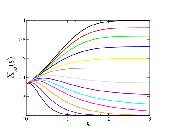
Figure 5: Plot of the asymptotic fluctuation-dissipation ratio $X_{\rm as}(s)$ in the critical regime in dimension three (see (10.31)) against the scaling variable $x=\mu\sqrt{2s}$, for the following values of the ratio $y/x=|{{\bf V}}|/\mu$ (top to bottom): 0 (reversible), 0.2, 0.3, 0.4, 0.5, $1/\sqrt{3}\approx 0.577350$ (so that $X_{\rm stat}(\infty)=1/2$), 0.7, 0.8, 0.9, 1 (borderline case), 1.2, 1.5 and 2.

The four-dimensional case ($\varepsilon=1$).

This situation corresponds to the upper critical dimension of the model, where the exponent $\nu$ changes from non-classical to classical (see (3.43)), so that logarithmic corrections to scaling can be expected a priori. The scaling function $h_{1}(\xi)$ is, however, a simple exponential (see (10.13)). As a consequence, to leading order in the critical regime, the quantities which can be expressed in terms of $h_{1}(\xi)$ are given for $D=4$ by their expressions in the classical regime ($D>4$), derived in section 9. In other words, logarithmic corrections to scaling are subleading for these quantities. This phenomenon was already put forward by Ebbinghaus et al [36]. In particular, the asymptotic fluctuation-dissipation ratio is given by (9.12), up to correction terms which are of the order of $1/\ln(1/\mu^{2})$, i.e., $1/|\ln(T-T_{c})|$, in relative value.

11 Ferromagnetic phase

This last section is devoted to the two-time observables of the model in its low-temperature ferromagnetic phase ($T<T_{c}$). This ordered phase only exists in high enough dimension ($D>2$). It is characterized by a non-zero value of the spontaneous magnetization $M_{\rm eq}$, given by (3.47).

The dynamical properties of the model in the late-time coarsening regime are ruled by the power-law decay (3.46) of the function $g(t)$. In particular, the behavior of the reduced dynamical susceptibility $\chi(t)=C^{\rm F}({\bf 0},t)$ can be estimated by keeping only the integral term in (3.13), and using (3.46) and the sum rule (3.48). We thus obtain

$$\chi(t)\approx M_{\rm eq}^{2}(8\pi t)^{D/2}.$$ (11.1)

This result has a simple interpretation: the typical linear size of a magnetized domain grows proportionally to the diffusive scale $L(t)\sim\sqrt{t}$ [1], so that its volume, measured by $\chi(t)$, grows as $L(t)^{D}\sim t^{D/2}$.

The commonly accepted phenomenology of glassy dynamics (see [37] for reviews) tells us that two-time quantities behave differently in the following two regimes, which will be studied successively hereafter:

• a beta (stationary) regime ($\tau=t-s\ll s$), where the two-time correlation function $C(t,s)$ only depends on $\tau$, and decays from unity to its plateau value $M_{\rm eq}^{2}$.

• an alpha (aging) regime ($\tau\sim s$), where the two-time correlation function further decays from its plateau value $M_{\rm eq}^{2}$ to zero.

11.1 Beta (stationary) regime

In this first regime, i.e., for $\tau\ll s$, it is legitimate to simplify (4.3) and (4.10) to

$$C_{\rm beta}^{\rm F}({\bf q},\tau) \approx \frac{T}{\omega({\bf q})}\,{\rm e}^{-\Omega({\bf q})\tau},$$

$$R_{\rm beta}^{\rm F}({\bf q},\tau) \approx {\rm e}^{-\Omega({\bf q})\tau}.$$ (11.2)

These expressions coincide with the $\mu\to 0$ limit of (5.2), which was shown to also describe the nonequilibrium stationary state at the critical point.

The correlation function therefore behaves as

$$C_{\rm beta}(\tau)\approx M_{\rm eq}^{2}+(1-M_{\rm eq}^{2})\Phi(\tau),$$ (11.3)

where the function

$$\Phi(\tau)=T_{c}\int\!{\frac{{\rm d}^{D}{\bf q}}{(2\pi)^{D}}}\frac{{\rm e}^{-\Omega({\bf q})\tau}}{\omega({\bf q})}$$ (11.4)

decreases from $\Phi(0)=1$ to $\Phi(\infty)=0$, and thus describes the relaxation of correlations throughout the beta regime.

Hereafter we focus our attention onto the scaling regime where ${{\bf V}}$ is small. The response function assumes the simple expression

$$R_{\rm beta}(\tau)\approx\frac{{\rm e}^{-{{\bf V}}^{2}\tau}}{(4\pi\tau)^{D/2}},$$ (11.5)

and therefore falls off exponentially to zero.

More interestingly, the tail of the function $\Phi(\tau)$, describing how the correlation function tends to its plateau value $M_{\rm eq}^{2}$, assumes the scaling form

$$\Phi(\tau)\approx\frac{T_{c}}{(4\pi)^{D/2}\tau^{(D-2)/2}}\,F(z),$$ (11.6)

where the scaling variable is

$$z={{\bf V}}^{2}\tau,$$ (11.7)

and with

$$F(z)=z^{-(D-2)/2}\;\gamma\left(\frac{D-2}{2},z\right),$$ (11.8)

where

$$\gamma(a,x)=\int_{0}^{x}{\rm d}y\,{\rm e}^{-y}y^{a-1}$$ (11.9)

is the incomplete Gamma function. The scaling function $F(z)$ starts from the finite value $F(0)=2/(D-2)$, and decays as $F(z)\approx\Gamma((D-2)/2)z^{-(D-2)/2}$ at large $z$. As a consequence, we have

$$\Phi(\tau)\approx\frac{2T_{c}}{(D-2)(4\pi)^{D/2}\tau^{(D-2)/2}}$$ (11.10)

for reversible dynamics (${{\bf V}}={\bf 0}$), and

$$\Phi(\tau)\approx\frac{T_{c}\,\Gamma((D-2)/2)}{(4\pi)^{D/2}(|{{\bf V}}|\tau)^{D-2}}$$ (11.11)

as soon as ${{\bf V}}\neq{\bf 0}$.

The correlation function therefore always exhibits a slow power-law convergence toward its plateau value. The exponent of this power law however depends on whether the dynamics is reversible or not. In the first case (see (11.10)), it equals $(D-2)/2$; in the second case (see (11.11)), its value is doubled to $D-2$.

Finally, in the same scaling regime where ${{\bf V}}$ is small and $\tau$ is large, the fluctuation-dissipation ratio also assumes a scaling form, namely

$$X_{\rm beta}(\tau)\approx{\cal X}(z),$$ (11.12)

with

$${\cal X}(z)=\frac{2\,{\rm e}^{-z}}{(D-2)F(z)-2zF^{\prime}(z)}.$$ (11.13)

The fluctuation-dissipation ratio is identically equal to unity for reversible dynamics (${{\bf V}}={\bf 0}$) throughout the beta regime. In the irreversible case, it starts decreasing as

$${\cal X}(z)=1-\frac{4z}{D}+\cdots,$$ (11.14)

i.e., $X_{\rm beta}(\tau)\approx 1-4{{\bf V}}^{2}\tau/D$, whereas it falls off roughly exponentially at large $z$.

To close, we give explicit expressions for the scaling functions $F(z)$ and ${\cal X}(z)$ in dimension three and four:

$$D=3:\quad F(z)=\sqrt{\frac{\pi}{z}}\mathop{\rm erf}\nolimits\sqrt{z},\quad{\cal X}(z)=\displaystyle{\displaystyle\sqrt{z}\over\displaystyle\sqrt{\pi}{\rm e}^{z}\mathop{\rm erf}\nolimits\sqrt{z}-\sqrt{z}},$$

$$D=4:\quad F(z)=\frac{1-{\rm e}^{-z}}{z},{\hskip 23.0pt}{\cal X}(z)=\frac{z}{2({\rm e}^{z}-1)-z}.$$ (11.15)

Figure 6 shows a plot of the scaling function ${\cal X}(z)$ for $D=3$ and $D=4$.

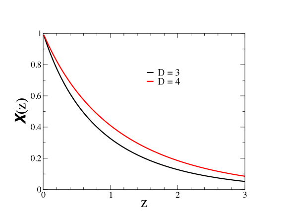
Figure 6: Plot of the scaling function ${\cal X}(z)$ describing the fluctuation-dissipation ratio in the beta regime in the ferromagnetic phase, against $z={{\bf V}}^{2}\tau$, for $D=3$ and $D=4$.

11.2 Alpha (aging) regime

Let us again consider, for the sake of simplicity, the scaling regime where ${{\bf V}}$ is small. Throughout the alpha (aging) regime, where both times $s$ and $t$ are large and comparable, (3.13), (4.3) and (4.10), together with (3.46) and the sum rule (3.48), lead to the estimates

$$C_{\rm alpha}(t,s) \approx M_{\rm eq}^{2}\left(\frac{4ts}{(t+s)^{2}}\right)^{D/4}{\rm e}^{-{{\bf V}}^{2}(t-s)^{2}/(t+s)},$$

$$R_{\rm alpha}(t,s) \approx \frac{{\rm e}^{-{{\bf V}}^{2}(t-s)}}{(4\pi(t-s))^{D/2}}\left(\frac{t}{s}\right)^{D/4},$$ (11.16)

which bear a strong resemblance with the formulas (8.14) pertaining to the zero-temperature dynamics of the one-dimensional model.

The corresponding fluctuation-dissipation ratio reads

$$X_{\rm alpha}(t,s) \approx \frac{4T}{D(8\pi)^{D/2}M_{\rm eq}^{2}}\left(\frac{t+s}{t-s}\right)^{(D+2)/2}s^{-(D-2)/2}$$ (11.17)

$$\times \frac{D(t+s)}{D(t+s)+4{{\bf V}}^{2}s(3t+s)}\,{\rm e}^{-2{{\bf V}}^{2}s(t-s)/(t+s)}.$$

The first line is the known result for reversible dynamics [15, 22], whereas the second one describes the effect of a (small) velocity ${{\bf V}}$ in the aging regime.

12 Discussion

We have introduced a spatial asymmetry into the linear Langevin dynamics for the ferromagnetic spherical model on the hypercubic lattice. The asymmetry is measured by an arbitrary velocity vector ${{\bf V}}$. The resulting dynamics is irreversible. It therefore breaks detailed balance and its numerous consequences, including the fluctuation-dissipation theorem. The corresponding nonequilibrium stationary state is however still Gibbsian, with the weights of configurations being dictated by the ferromagnetic Hamiltonian.

The model remains exactly solvable in any dimension, allowing thus an analytical evaluation of time-dependent observables. The main emphasis has been put on two-time quantities, and especially on the fluctuation-dissipation ratio. We have performed a systematic investigation of several regimes of interest, either stationary or transient, for arbitrary dimensions and in the different phases of the model. One of the most noticeable outcomes of this study is the existence of two regimes of violation of the fluctuation-dissipation theorem in the nonequilibrium stationary state: a regime of weak violation at small ${{\bf V}}$, where the stationary value of the fluctuation-dissipation ratio is finite but less than unity, and varies continuously with ${{\bf V}}$, and a regime of strong violation at large ${{\bf V}}$, where the fluctuation-dissipation ratio vanishes asymptotically. This phenomenon had been uncovered for the first time in the kinetic Ising chain under asymmetric dynamics [11]. The present study suggests that this novel kind of dynamical transition in nonequilibrium stationary states might be quite general. We have also characterized the rounding of the above transition in the transient regime.

As mentioned in the introduction, numerical simulations of the two-dimensional Ising model with the asymmetric dynamics introduced in [10] are currently in progress [12]. Finally, it would be worth pursuing the exploration of irreversible dynamics and nonequilibrium stationary states driven by spatial asymmetries in other directions, such as conserved dynamics, or with other approaches, such as field-theoretical methods.

Acknowledgments

It is a pleasure to thank Malte Henkel for interesting discussions during preliminary stages of this work.

References

References

- [1] Bray A J, 1994 Adv. Phys. 43 357
- [2] Glauber R G, 1963 J. Math. Phys. 4 294
- [3] Godrèche C and Luck J M, 2000 J. Phys. A 33 1151
- [4] Lippiello E and Zannetti M, 2000 Phys. Rev. E 61 3369
- [5] Mayer P and Sollich P, 2004 J. Phys. A 37 9
- [6] Henkel M and Pleimling M, 2010 Nonequilibrium Phase Transitions Volume 2: Ageing and Dynamical Scaling far from Equilibrium (Heidelberg: Springer)
- [7] Katz S, Lebowitz J L and Spohn H, 1983 Phys. Rev. B 28 1655 Katz S, Lebowitz J L and Spohn H, 1984 J. Stat. Phys. 34 497 Schmittmann B and Zia R K P, 1995 Statistical Mechanics of Driven Diffusive Systems Phase Transitions and Critical Phenomena 17 eds Domb C and Lebowitz J L (New York: Academic)
- [8] Künsch H R, 1984 Z. Wahr. verw. Gebiete 66 407
- [9] Lima F W S and Stauffer D, 2006 Physica A 359 423
- [10] Godrèche C and Bray A J, 2009 J. Stat. Mech. P12016
- [11] Godrèche C, 2011 J. Stat. Mech. P04005
- [12] Godrèche C and Pleimling M, in preparation
- [13] Maes C, Redig F and Van Moffaert A, 2000 J. Math. Phys. 41 1528
- [14] de Oliveira M J, 2011 J. Stat. Mech. P12012
- [15] Godrèche C and Luck J M, 2000 J. Phys. A 33 9141 Godrèche C and Luck J M, 2002 J. Phys. Cond. Matt. 14 1589
- [16] Berlin T H and Kac M, 1952 Phys. Rev. 86 821
- [17] Stanley H E, 1968 Phys. Rev. 176 718
- [18] Baxter R J, 1982 Exactly Solved Models in Statistical Mechanics (London: Academic)
- [19] Ronca G, 1978 J. Chem. Phys. 68 3737
- [20] Janssen H K, Schaub B and Schmittmann B, 1989 Z. Phys. B 73 539
- [21] Cugliandolo L F and Dean D S, 1995 J. Phys. A 28 4213
- [22] Zippold W, Kühn R and Horner H, 2000 Eur. Phys. J. B 13 531
- [23] Cannas S A, Stariolo D A and Tamarit F A, 2001 Physica A 294 362 Picone A and Henkel M, 2002 J. Phys. A 35 5575 Picone A, Henkel M and Richert J, 2003 J. Phys. A 36 1249 Paessens M and Henkel M, 2003 J. Phys. A 36 8983 Baumann F and Pleimling M, 2006 J. Phys. A 39 1981 Hase M O and Salinas S R, 2006 J. Phys. A 39 4875 Baumann F, Dutta S B and Henkel M, 2007 J. Phys. A 40 7389 Annibale A and Sollich P, 2009 J. Stat. Mech. P02064
- [24] Crisanti A, Horner H and Sommers H J, 1993 Z. Phys. B 92 257 Biroli G, 1999 J. Phys. A 32 8365 Kim B and Latz A, 2001 Europhys. Lett. 53 660 Chamon C, Cugliandolo L F and Yoshino H, 2006 J. Stat. Mech. P01006 Ferrari U, Leuzzi L, Parisi G and Rizzo T, 2012 Phys. Rev. B 86 014204
- [25] Crisanti A and Sompolinsky H, 1987 Phys. Rev. A 36 4922
- [26] Hase M O and de Oliveira M J, 2012 J. Phys. A 45 165003
- [27] Lewis H W and Wannier G H, 1952 Phys. Rev. 88 682 Lewis H W and Wannier G H, 1953 Phys. Rev. 90 1131 (erratum)
- [28] Kubo R, 1966 Rep. Prog. Phys. 29 255 Marconi U M B, Puglisi A, Rondoni L and Vulpiani A, 2008 Phys. Rep. 461 111
- [29] Chandler D, 1987 Introduction to Modern Statistical Mechanics (New York: Oxford University Press)
- [30] Cugliandolo L F and Kurchan J, 1993 Phys. Rev. Lett. 71 173 Cugliandolo L F, Kurchan J and Parisi G, 1994 J. Phys. I (France) 4 1641 Cugliandolo L F and Kurchan J, 1994 J. Phys. A 27 5749 Cugliandolo L F, Kurchan J and Peliti L, 1997 Phys. Rev. E 55 3898 Cugliandolo L F and Kurchan J, 2000 J. Phys. Soc. Japan 69 (Suppl A) 247
- [31] Crisanti A and Ritort F, 2003 J. Phys. A 36 R181 Corberi F, Lippiello E and Zannetti M, 2007 J. Stat. Mech. P07002 Leuzzi L, 2009 J. Non-Cryst. Solids 355 686 Cugliandolo L F, 2011 J. Phys. A 44 483001
- [32] Calabrese P and Gambassi A, 2005 J. Phys. A 38 R133
- [33] Godrèche C, unpublished
- [34] Luck J M and Mehta A, 2001 Europhys. Lett. 54 573
- [35] Hardy G H, 1940 Ramanujan (Cambridge: Cambridge University Press) pp 195-198
- [36] Ebbinghaus M, Grandclaude H and Henkel M, 2008 Eur. Phys. J. B 63 85
- [37] Vincent E, Hammann J, Ocio M, Bouchaud J P and Cugliandolo L F, 1997 Lect. Notes Phys. 492 184 (Berlin: Springer) Bouchaud J P, Cugliandolo L F, Kurchan J and Mézard M, 1998 Directions in Condensed Matter Physics 12 Young A P ed (Singapore: World Scientific) Berthier L, Biroli G, Bouchaud J P, Cipelletti L and van Saarloos W (eds), 2011 Dynamical Heterogeneities in Glasses, Colloids, and Granular Media International Series of Monographs on Physics (Oxford: Oxford University Press)