Upper Bounds on the Size of Grain-Correcting Codes^∗

Abstract.

In this paper, we re-visit the combinatorial error model of Mazumdar et al. [3] that models errors in high-density magnetic recording caused by lack of knowledge of grain boundaries in the recording medium. We present new upper bounds on the cardinality/rate of binary block codes that correct errors within this model.

1. Introduction

The combinatorial error model studied by Mazumdar et al. [3] is a highly simplified model of an error mechanism encountered in a magnetic recording medium at terabit-per-square-inch storage densites [4], [7]. In this model, a one-dimensional track on a magnetic recording medium is divided into evenly spaced bit cells, each of which can store one bit of data. Bits are written sequentially into these bit cells. The sequence of bit cells has an underlying “grain” distribution, which may be described as follows: bit cells are grouped into non-overlapping blocks called grains, which may consist of up to $b$ adjacent bit cells. We focus on the case $b=2$, so that a grain can contain at most two bit cells. We define the length of a grain to be the number of bit cells it contains.

Each grain can store only one bit of information, i.e., all the bit cells within a grain carry the same bit value (0 or 1), which we call the polarity of the grain. We assume, following [3], that in the sequential write process, the first bit to be written into a grain sets the polarity of the grain, so that all the bit cells within this grain must retain this polarity. This implies that any subsequent attempts at writing bits within this grain make no difference to the value actually stored in the bit cells in the grain. If the grain boundaries were known to the write head (encoder) and the read head (decoder), then the maximum storage capacity of one bit per grain can be achieved. However, in a more realistic scenario where the underlying grain distribution is fixed but unknown, the lack of knowledge of grain boundaries reduces the storage capacity. Constructions and rate/cardinality bounds for codes that correct errors caused by a fixed but unknown underlying grain distribution have been studied in the prior literature [3], [5], [6]. In this paper, we present improved rate/cardinality upper bounds for such codes.

The paper is organized as follows. After providing the necessary definitions and notation in Section 2, we derive, in Section 3, an upper bound on the cardinality of $t$-grain-correcting codes, for $t=1,2,3$, using the fractional covering technique from [1]. We conjecture that the upper bound in fact holds for all $t$. We further conjecture that the same technique should yield a stronger upper bound, and we report some progress towards this in Section 4. The fractional covering technique is also used in Section 5 to obtain an upper bound on the maximum rate asymptotically achievable by codes correcting a constant fraction of grain errors. An information-theoretic upper bound on the same quantity is derived in Section 6. We conclude in Section 7 with some remarks concerning the bounds. The current state-of-the-art on upper bounds on the maximum rate asymptotically achievable, including the bounds derived in this paper, is summarized in Figures 2 and 3. Some of the technical proofs from Sections 3 and 5 are given in appendices.

2. Definitions and Notation

Let $\Sigma=\{0,1\}$, and for a positive integer $n$, let $[n]$ denote the set $\{1,2,\ldots,n\}$. A track on the recording medium consists of $n$ bit cells indexed by the integers in $[n]$. The bit cells on the track are grouped into non-overlapping grains of length at most two. A length-2 grain consists of bit cells with indices $j-1$ and $j$, for some $j\in[n]$; we denote such a grain by the pair $(j-1,j)$. Let $E\subseteq\{2,\ldots,n\}$ be the set of all indices $j$ such that $(j-1,j)$ is a length-2 grain. Since grains cannot overlap, $E$ contains no pair of consecutive integers.

A binary sequence ${\mathbf{x}}=(x_{1},\ldots,x_{n})\in\Sigma^{n}$ to be written on to the track can be affected by errors only at the indices $j\in E$. Indeed, what actually gets recorded on the track is the sequence ${\mathbf{y}}=(y_{1},\ldots,y_{n})$, where

$$y_{j}=\begin{cases}x_{j-1}&\text{ if }j\in E\\ x_{j}&\text{ otherwise. }\end{cases}$$ (1)

For example, if ${\mathbf{x}}=(000101011100010)$ and $E=\{2,4,7,9,14\}$, then ${\mathbf{y}}=(000001111100000)$. Note that the set $E$ completely specifies the positions and locations of all the grains (both length-1 and length-2) in the track. We will call this set the grain pattern. It is assumed that the grain pattern is unknown to both the write head and the read head. The effect of the grain pattern $E$ on a binary sequence ${\mathbf{x}}\in\Sigma^{n}$ defines an operator $\phi_{E}:\Sigma^{n}\to\Sigma^{n}$, where ${\mathbf{y}}=\phi_{E}({\mathbf{x}})$ is as specified by (1) above.

For integers $n\geq 1$ and $t\geq 0$, let ${\mathcal{E}}_{n,t}$ denote the set of all grain patterns $E$ with $|E|\leq t$. In other words, ${\mathcal{E}}_{n,t}$ consists of all subsets $E\subseteq\{2,\ldots,n\}$ of cardinality at most $t$, such that $E$ contains no pair of consecutive integers. For an ${\mathbf{x}}\in\Sigma^{n}$, we define

$$\Phi_{t}({\mathbf{x}})=\{\phi_{E}({\mathbf{x}}):E\in{\mathcal{E}}_{n,t}\}.$$

Thus, $\Phi_{t}({\mathbf{x}})$ is the set of all possible sequences that can be obtained from ${\mathbf{x}}$ by the action of some grain pattern $E$ with $|E|\leq t$. Two sequences ${\mathbf{x}}_{1}$ and ${\mathbf{x}}_{2}$ are $t$-confusable if $\Phi_{t}({\mathbf{x}}_{1})\cap\Phi_{t}({\mathbf{x}}_{2})\neq\emptyset$. A binary code ${\mathcal{C}}$ of length $n$ is said to correct $t$ grain errors, or be a $t$-grain-correcting code, if no two distinct vectors ${\mathbf{x}}_{1},{\mathbf{x}}_{2}\in{\mathcal{C}}$ are $t$-confusable. Let $M(n,t)$ denote the maximum cardinality of a $t$-grain-correcting code of length $n$. Also, for $\tau\in[0,\frac{1}{2}]$, the maximum asymptotic rate of a $\lceil{\tau n}\rceil$-grain-correcting code is defined to be

$$R(\tau)=\limsup_{n\to\infty}\frac{1}{n}\,\log_{2}M(n,\lceil\tau n\rceil).$$ (2)

A grain pattern $E$ changes a sequence ${\mathbf{x}}$ to a different sequence ${\mathbf{y}}$ iff $x_{j-1}\neq x_{j}$ for some $j\in E$, i.e., the length-2 grain $(j-1,j)$ straddles the boundary between two successive runs in ${\mathbf{x}}$. Here, a run is a maximal substring of consecutive identical symbols ($0$s or $1$s) in ${\mathbf{x}}$. A run consisting of $0$s (resp. $1$s) is called a $0$-run (resp. $1$-run). The number of distinct runs in ${\mathbf{x}}$ is denoted by $r({\mathbf{x}})$.

A convenient means of keeping track of run boundaries in ${\mathbf{x}}$ is via its derivative sequence, ${\mathbf{x}}^{\prime}$: for ${\mathbf{x}}=(x_{1},\ldots,x_{n})$, the sequence ${\mathbf{x}}^{\prime}=(x^{\prime}_{2},\ldots,x^{\prime}_{n})$ is defined by $x^{\prime}_{j}=x_{j-1}\oplus x_{j}$, $j=2,\ldots,n$, where $\oplus$ denotes modulo-2 addition. The $1$s in ${\mathbf{x}}^{\prime}$ identify the boundaries between successive runs in ${\mathbf{x}}$. Thus, $\omega({\mathbf{x}}^{\prime})=r({\mathbf{x}})-1$, where $\omega(\cdot)$ denotes the Hamming weight of a binary sequence.

Let ${\text{supp}}({\mathbf{x}}^{\prime})=\{j:x^{\prime}_{j}=1\}$ denote the support of ${\mathbf{x}}^{\prime}$. For ${\mathbf{x}}\in\Sigma^{n}$, the sequences ${\mathbf{y}}\in\Phi_{t}({\mathbf{x}})$ are in one-to-one correspondence with the different ways of selecting at most $t$ non-consecutive integers from ${\text{supp}}({\mathbf{x}}^{\prime})$ to form a grain pattern $E\in{\mathcal{E}}_{n,t}$. Thus, $|\Phi_{t}({\mathbf{x}})|$ counts the number of ways of forming such grain patterns. This count can be obtained as follows. Let $\ell_{1},\ell_{2},\ldots,\ell_{m}$ denote the lengths of the distinct $1$-runs in ${\mathbf{x}}^{\prime}$, and define the set

$$T=\bigl{\{}(t_{1},\ldots,t_{m})\in{\mathbb{Z}}_{+}^{m}:\sum_{j=1}^{m}t_{j}\leq t\bigr{\}},$$ (3)

where ${\mathbb{Z}}_{+}$ denotes the set of non-negative integers. In the above expression, $t_{j}$ represents the number of integers from the support of the $j$th 1-run that are to be included in a grain pattern $E$ being formed. The number of distinct ways in which $t_{j}$ non-consecutive integers can be chosen from the $\ell_{j}$ consecutive integers forming the support of the $j$th $1$-run is, by an elementary counting argument, equal to $\binom{\ell_{j}-t_{j}+1}{t_{j}}$. Thus,

$$|\Phi_{t}({\mathbf{x}})|=\sum_{(t_{1},\ldots,t_{m})\in T}\prod_{j=1}^{m}\binom{\ell_{j}-t_{j}+1}{t_{j}}.$$ (4)

Simplified expressions can be obtained for small values of $t$.

Proposition 2.1.

For ${\mathbf{x}}\in\Sigma^{n}$, let $\omega=\omega({\mathbf{x}}^{\prime})$ denote the Hamming weight of the derivative sequence ${\mathbf{x}}^{\prime}$. Also, let $m$ be the number of 1-runs in ${\mathbf{x}}^{\prime}$.

• $|\Phi_{1}({\mathbf{x}})|=1+\omega=r({\mathbf{x}})$.

• $|\Phi_{2}({\mathbf{x}})|=1+m+\binom{\omega}{2}$.

• $|\Phi_{3}({\mathbf{x}})|=1+m_{1}+m(\omega-3)+\binom{\omega}{3}-\binom{\omega}{2}+2\omega$, where $m_{1}$ denotes the number of 1-runs of length 1 in ${\mathbf{x}}^{\prime}$.

Proof.

(a) While the expression for $|\Phi_{1}({\mathbf{x}})|$ can be directly obtained from (4), it is simpler to observe that the set $\Phi_{1}({\mathbf{x}})$ consists of the sequence ${\mathbf{x}}$ itself, and the $\omega$ distinct sequences in the set $\bigl{\{}\phi_{E}({\mathbf{x}}):E=\{j\}\text{ for some }j\in{\text{supp}}({\mathbf{x}}^{\prime})\bigr{\}}$.

(b) For $t=2$, it is easy to see that the expression in (4) simplifies to

$$|\Phi_{2}({\mathbf{x}})|=1+\sum_{j=1}^{m}\ell_{j}+\sum_{j=1}^{m}\binom{\ell_{j}-1}{2}+\sum_{(i,j):i<j}\ell_{i}\ell_{j}.$$

We then have

$$|\Phi_{2}({\mathbf{x}})| = 1+m+\sum_{j=1}^{m}(\ell_{j}-1)+\sum_{j=1}^{m}\binom{\ell_{j}-1}{2}+\sum_{(i,j):i<j}\ell_{i}\ell_{j}$$

$$= 1+m+\sum_{j=1}^{m}\binom{\ell_{j}}{2}+\sum_{(i,j):i<j}\ell_{i}\ell_{j}$$

$$= 1+m+\frac{1}{2}\sum_{j=1}^{m}(\ell_{j}^{2}-\ell_{j})+\sum_{(i,j):i<j}\ell_{i}\ell_{j}$$

$$= 1+m+\frac{1}{2}\left[\sum_{j=1}^{m}\ell_{j}^{2}+\sum_{(i,j):i\neq j}\ell_{i}\ell_{j}-\sum_{j=1}^{m}\ell_{j}\right]$$

$$= 1+m+\frac{1}{2}\left[\biggl{(}\sum_{j=1}^{m}\ell_{j}\biggr{)}^{2}-\sum_{j=1}^{m}\ell_{j}\right]$$

$$= 1+m+\binom{\omega}{2},$$

the last equality being due to the fact that $\omega=\sum_{j=1}^{m}\ell_{j}$.

(c) For $t=3$, the expression in (4) can be written as

$$|\Phi_{3}({\mathbf{x}})|=|\Phi_{2}({\mathbf{x}})|+\sum_{(i,j,k):i<j<k}\ell_{i}\ell_{j}\ell_{k}+\sum_{i=1}^{m}\binom{\ell_{i}-1}{2}\biggl{(}\sum_{j:j\neq i}\ell_{j}\biggr{)}+\sum_{i=1}^{m}\binom{\ell_{i}-2}{3}.$$

From here on, straightforward algebraic manipulations lead to the expression given in the statement of the proposition. We omit the details, noting only that $m_{1}$ enters the picture when we write the last term above as

$$\sum_{i=1}^{m}\frac{(\ell_{i}-2)(\ell_{i}-3)(\ell_{i}-4)}{6}+\sum_{i:\ell_{i}=1}1.$$

The extra term $\sum_{i:\ell_{i}=1}1$, which equals $m_{1}$, accounts for the fact that the expansion of $\binom{\ell_{i}-2}{3}$ as $\frac{(\ell_{i}-2)(\ell_{i}-3)(\ell_{i}-4)}{6}$ is invalid when $\ell_{i}=1$; by convention, $\binom{a}{b}=0$ when $a<0$. ∎

We will also find the following simple lower bound on $|\Phi_{t}({\mathbf{x}})|$, valid for any $t\geq 1$, to be useful.

Proposition 2.2.

For ${\mathbf{x}}\in\Sigma^{n}$ and $t\geq 1$, we have

$$|\Phi_{t}({\mathbf{x}})|\geq\sum_{j=0}^{t}\binom{r({\mathbf{x}})-j}{j}.$$

Proof.

Consider the number of different ways of choosing exactly $j$ non-consecutive integers from ${\text{supp}}({\mathbf{x}}^{\prime})$. This number is smallest when ${\text{supp}}({\mathbf{x}}^{\prime})$ consists of consecutive integers, e.g., ${\text{supp}}({\mathbf{x}})=[r({\mathbf{x}})-1]$. The number of different ways of choosing exactly $j$ non-consecutive integers from $[r({\mathbf{x}})-1]$ is, by an elementary counting argument, equal to $\binom{r({\mathbf{x}})-j}{j}$. ∎

3. An Upper Bound on $M(n,t)$

In this section, we explore the applicability to grain-correcting codes of a technique used by Kulkarni and Kiyavash [1] to derive upper bounds on the cardinalities of deletion-correcting codes.

A hypergraph ${\mathcal{H}}$ is a pair $(V,{\mathcal{X}})$, where $V$ is a finite set, called the vertex set, and ${\mathcal{X}}$ is a family of subsets of $V$. The members of ${\mathcal{X}}$ are called hyperedges. A matching of ${\mathcal{H}}$ is a pairwise disjoint collection of hyperedges. A (vertex) covering of ${\mathcal{H}}$ is a subset $T\subseteq V$ such that $T$ meets every hyperedge of ${\mathcal{H}}$, i.e., $T\cap X\neq\emptyset$ for all $X\in{\mathcal{X}}$. The matching number $\nu({\mathcal{H}})$ is the largest size of a matching of ${\mathcal{H}}$, while the covering number, $\tau({\mathcal{H}})$, is the smallest size of a covering of ${\mathcal{H}}$.

The problems of computing the matching and covering numbers can be expressed as a dual pair of integer programs. This is done via the vertex-hyperedge incidence matrix, $A$, of ${\mathcal{H}}$, which is defined as follows. Let $v_{1},v_{2},\ldots,v_{|V|}$ and $X_{1},X_{2},\ldots,X_{|{\mathcal{X}}|}$ be a listing of the vertices and hyperedges, respectively, of ${\mathcal{H}}$. Then, $A=(A_{i,j})$ is the $|V|\times|{\mathcal{X}}|$ matrix with $0/1$ entries, with $A_{i,j}=1$ iff $v_{i}\in X_{j}$. It is easy to verify that

$$\nu({\mathcal{H}})=\max\{{\mathbf{1}}^{T}{\mathbf{z}}:{\mathbf{z}}\in\{0,1\}^{|{\mathcal{X}}|},\ A{\mathbf{z}}\leq{\mathbf{1}}\}$$ (5)

and

$$\tau({\mathcal{H}})=\min\{{\mathbf{1}}^{T}{\mathbf{w}}:{\mathbf{w}}\in\{0,1\}^{|V|},\ A^{T}{\mathbf{w}}\geq{\mathbf{1}}\},$$ (6)

where ${\mathbf{1}}$ denotes an all-ones column vector. Note that the linear programming (LP) relaxations of (5),

$$\nu_{f}({\mathcal{H}})=\max\{{\mathbf{1}}^{T}{\mathbf{z}}:{\mathbf{z}}\geq{\mathbf{0}},\ A{\mathbf{z}}\leq{\mathbf{1}}\},$$ (7)

and (6),

$$\tau_{f}({\mathcal{H}})=\min\{{\mathbf{1}}^{T}{\mathbf{w}}:{\mathbf{w}}\geq{\mathbf{0}},\ A^{T}{\mathbf{w}}\geq{\mathbf{1}}\},$$ (8)

are duals of each other. By strong LP duality, we have $\nu_{f}({\mathcal{H}})=\tau_{f}({\mathcal{H}})$, and hence,

$$\nu({\mathcal{H}})\leq\nu_{f}({\mathcal{H}})=\tau_{f}({\mathcal{H}})\leq\tau({\mathcal{H}}).$$ (9)

The quantities $\nu_{f}({\mathcal{H}})$ and $\tau_{f}({\mathcal{H}})$ are called the fractional matching number and fractional covering number, respectively, of the hypergraph ${\mathcal{H}}$. Any non-negative vector ${\mathbf{w}}$ such that $A^{T}{\mathbf{w}}\geq 1$ is called a fractional covering of ${\mathcal{H}}$. To put it in another way, a fractional covering is a function ${\mathsf{w}}:V\to{\mathbb{R}}_{+}$ such that $\sum_{v\in X}{\mathsf{w}}(v)\geq 1$ for all $X\in{\mathcal{X}}$. The value of a fractional covering ${\mathsf{w}}$ is defined to be $|{\mathsf{w}}|:=\sum_{v\in V}{\mathsf{w}}(v)$. From the inequality $\nu({\mathcal{H}})\leq\tau_{f}({\mathcal{H}})$ in (9), we see that $\nu({\mathcal{H}})\leq|{\mathsf{w}}|$ for any fractional covering ${\mathsf{w}}$ of ${\mathcal{H}}$. We use this to suggest an upper bound on the largest size, $M(n,t)$, of a $t$-grain-correcting code of blocklength $n$.

Consider the hypergraph ${\mathcal{H}}_{n,t}=(V,{\mathcal{X}})$, where $V=\Sigma^{n}$, and ${\mathcal{X}}=\{\Phi_{t}({\mathbf{x}}):{\mathbf{x}}\in\Sigma^{n}\}$. Note that $\nu({\mathcal{H}}_{n,t})=M(n,t)$; thus, fractional coverings of ${\mathcal{H}}_{n,t}$ yield upper bounds on $M(n,t)$. Bounding the size of packings in this way has been extensively used in combinatorics, see e.g. [2]. Taking inspiration from [1], we consider the function ${\mathsf{w}}_{t}:\Sigma^{n}\to{\mathbb{R}}_{+}$, defined for ${\mathbf{x}}\in\Sigma^{n}$ as

$${\mathsf{w}}_{t}({\mathbf{x}})=\frac{1}{|\Phi_{t}({\mathbf{x}})|}.$$ (10)

For $t=1,2,3$, we can prove that ${\mathsf{w}}_{t}$ is a fractional covering of ${\mathcal{H}}_{n,t}$, and conjecture that this is in fact the case for all $t\geq 1$.

Conjecture 3.1.

For all positive integers $n$ and $t$, the function ${\mathsf{w}}_{t}$ defined in (10) is a fractional covering of ${\mathcal{H}}_{n,t}$, i.e., for all ${\mathbf{x}}\in\Sigma^{n}$,

$$\sum_{{\mathbf{y}}\in\Phi_{t}({\mathbf{x}})}\frac{1}{|\Phi_{t}({\mathbf{y}})|}\geq 1.$$ (11)

Therefore,

$$M(n,t)\leq|{\mathsf{w}}_{t}|=\sum_{{\mathbf{x}}\in\Sigma^{n}}\frac{1}{|\Phi_{t}({\mathbf{x}})|}.$$ (12)

Our proof of (11) for $t=1,2,3$ relies on an understanding of the relationship between $|\Phi_{t}({\mathbf{x}})|$ and $|\Phi_{t}({\mathbf{y}})|$ for ${\mathbf{y}}\in\Phi_{t}({\mathbf{x}})$. Recall, from (4), that $|\Phi_{t}({\mathbf{x}})|$ depends only on the lengths of the 1-runs in ${\mathbf{x}}^{\prime}$. Thus, we need to understand how the distribution of 1s changes in going from ${\mathbf{x}}^{\prime}$ to ${\mathbf{y}}^{\prime}$.

3.1. Effect of Grains on the Derivative Sequence

Recall that $1$s in ${\mathbf{x}}^{\prime}$ correspond to run boundaries in ${\mathbf{x}}$. We say that a (length-2) grain acts on a $1$ in ${\mathbf{x}}^{\prime}$ if it straddles the corresponding run boundary in ${\mathbf{x}}$. We need to distinguish between two types of 1s in the derivative sequence ${\mathbf{x}}^{\prime}$. A trailing $1$ is the last $1$ in a $1$-run, while a non-trailing $1$ is any $1$ that is not a trailing $1$. Grains act on trailing $1$s in a manner different from non-trailing $1$s.

A segment of ${\mathbf{x}}^{\prime}$ that contains a trailing $1$ is of the form $*10*$, or $*1$ in case the trailing $1$ is a suffix of ${\mathbf{x}}$. Up to complementation, the corresponding segment of ${\mathbf{x}}$ is of the form $*011*$ or $*01$. A grain acting on the trailing $1$ in ${\mathbf{x}}^{\prime}$ straddles the $01$ run boundary in ${\mathbf{x}}$. In the sequence ${\mathbf{y}}$ obtained through the action of this grain, the segment under observation becomes $*001*$ or $*00$, and the corresponding segment of the derivative sequence ${\mathbf{y}}^{\prime}$ is $*01*$ or $*0$.

On the other hand, a non-trailing $1$ in ${\mathbf{x}}^{\prime}$ belongs to a segment of the form $*11*$; the first $1$ shown is the non-trailing $1$ under consideration. Again, up to complementation, the corresponding segment in ${\mathbf{x}}$ is of the form $*010*$. A grain acting on the non-trailing $1$ in ${\mathbf{x}}^{\prime}$ straddles the $01$ run boundary shown in ${\mathbf{x}}$. This grain causes the segment being observed to become $*000*$ in ${\mathbf{y}}$, and hence $*00*$ in ${\mathbf{y}}^{\prime}$.

To summarize, the action of a grain on a trailing $1$ converts a segment of the form $*10*$ or $*1$ in ${\mathbf{x}}^{\prime}$ to $*01*$ or $*0$ in ${\mathbf{y}}^{\prime}$, and a grain acting on a non-trailing $1$ converts a segment of the form $*11*$ in ${\mathbf{x}}^{\prime}$ to $*00*$ in ${\mathbf{y}}^{\prime}$. It should be clear that the bits depicted by $*$s on either side of these segments remain unchanged by the action of the grain. Note, in particular, that a grain acting on a $1$ in ${\mathbf{x}}^{\prime}$ does not increase the Hamming weight of ${\mathbf{x}}^{\prime}$. A grain acting on a trailing $1$ either leaves the Hamming weight of ${\mathbf{x}}^{\prime}$ unchanged, or reduces it by $1$; in the case of a non-trailing $1$, the Hamming weight of ${\mathbf{x}}^{\prime}$ is always reduced by $2$.

Finally, when dealing with a grain pattern containing $t>1$ length-2 grains, since the grains are non-overlapping, the actions of individual grains can be considered independently. Thus, the discussion above immediately implies the following useful fact.

Lemma 3.1.

For any ${\mathbf{y}}\in\Phi_{t}({\mathbf{x}})$, we have $\omega({\mathbf{y}}^{\prime})\leq\omega({\mathbf{x}}^{\prime})$, or equivalently, $r({\mathbf{y}})\leq r({\mathbf{x}})$.

3.2. Proof of (11) for $t=1,2,3$

Consider $t=1$ first. For any ${\mathbf{y}}\in\Phi_{1}({\mathbf{x}})$, we have $\omega({\mathbf{y}}^{\prime})\leq\omega({\mathbf{x}}^{\prime})$, and hence, $|\Phi_{1}({\mathbf{y}})|\leq|\Phi_{1}({\mathbf{x}})|$ by Proposition 2.1. Therefore,

$$\sum_{{\mathbf{y}}\in\Phi_{1}({\mathbf{x}})}\frac{1}{|\Phi_{1}({\mathbf{y}})|}\geq\sum_{{\mathbf{y}}\in\Phi_{1}({\mathbf{x}})}\frac{1}{|\Phi_{1}({\mathbf{x}})|}=1,$$

which proves $(\ref{eq:sum_y})$ for $t=1$.

The simple argument above does not extend directly to $t\geq 2$, the reason being that it is no longer true in general that $|\Phi_{t}({\mathbf{y}})|\leq|\Phi_{t}({\mathbf{x}})|$ for ${\mathbf{y}}\in\Phi_{t}({\mathbf{x}})$. For example, consider ${\mathbf{x}}=0100$, and note that $\Phi_{2}({\mathbf{x}})=\{0000,0100,0110\}$. Take ${\mathbf{y}}=0110\in\Phi_{2}({\mathbf{x}})$, and verify that $\Phi_{2}({\mathbf{y}})=\{0110,0010,0111,0011\}$. Thus, $|\Phi_{2}({\mathbf{y}})|>|\Phi_{2}({\mathbf{x}})|$.

To prove (11) for $t=2,3$, we show that the sequences ${\mathbf{y}}\in\Phi_{t}({\mathbf{x}})$ that violate the inequality $|\Phi_{t}({\mathbf{y}})|\leq|\Phi_{t}({\mathbf{x}})|$ can be dealt with by suitably matching them with sequences that satisfy the inequality. To this end, for a fixed ${\mathbf{x}}\in\Sigma^{n}$, let us define $F_{t}({\mathbf{x}})=\{{\mathbf{y}}\in\Phi_{t}({\mathbf{x}}):|\Phi_{t}({\mathbf{y}})|>|\Phi_{t}({\mathbf{x}})|\}$ and $G_{t}({\mathbf{x}})=\{{\mathbf{y}}\in\Phi_{t}({\mathbf{x}}):|\Phi_{t}({\mathbf{y}})|\leq|\Phi_{t}({\mathbf{x}})|\}$. We will construct a one-to-one mapping $p:F_{t}({\mathbf{x}})\to G_{t}({\mathbf{x}})$ such that for all ${\mathbf{y}}\in F_{t}({\mathbf{x}})$, we have

$$\frac{1}{|\Phi_{t}({\mathbf{y}})|}+\frac{1}{|\Phi_{t}(p({\mathbf{y}}))|}\geq\frac{2}{|\Phi_{t}({\mathbf{x}})|}.$$ (13)

The mapping $p$ will be referred to as a pairing. Let $P_{t}({\mathbf{x}})=p(F_{t}({\mathbf{x}}))$ denote the image of $p$, and let $Q_{t}({\mathbf{x}})=G_{t}({\mathbf{x}})\setminus P_{t}({\mathbf{x}})$. Thus, $|P_{t}({\mathbf{x}})|=|F_{t}({\mathbf{x}})|$, and $\Phi_{t}({\mathbf{x}})=F_{t}({\mathbf{x}})\stackrel{{\scriptstyle\cdot}}{{\cup}}P_{t}({\mathbf{x}})\stackrel{{\scriptstyle\cdot}}{{\cup}}Q_{t}({\mathbf{x}})$. Then,

$$\sum_{{\mathbf{y}}\in\Phi_{t}({\mathbf{x}})}\frac{1}{|\Phi_{t}({\mathbf{y}})|} = \sum_{{\mathbf{y}}\in F_{t}({\mathbf{x}})}\frac{1}{|\Phi_{t}({\mathbf{y}})|}+\sum_{{\mathbf{y}}\in P_{t}({\mathbf{x}})}\frac{1}{|\Phi_{t}({\mathbf{y}})|}+\sum_{{\mathbf{y}}\in Q_{t}({\mathbf{x}})}\frac{1}{|\Phi_{t}({\mathbf{y}})|}$$

$$= \sum_{{\mathbf{y}}\in F_{t}({\mathbf{x}})}\frac{1}{|\Phi_{t}({\mathbf{y}})|}+\sum_{{\mathbf{y}}\in F_{t}({\mathbf{x}})}\frac{1}{|\Phi_{t}(p({\mathbf{y}}))|}+\sum_{{\mathbf{y}}\in Q_{t}({\mathbf{x}})}\frac{1}{|\Phi_{t}({\mathbf{y}})|}$$

$$\geq \sum_{{\mathbf{y}}\in F_{t}({\mathbf{x}})}\frac{2}{|\Phi_{t}({\mathbf{x}})|}+\sum_{{\mathbf{y}}\in Q_{t}({\mathbf{x}})}\frac{1}{|\Phi_{t}({\mathbf{x}})|}$$

$$= \frac{1}{|\Phi_{t}({\mathbf{x}})|}\,(2|F_{t}({\mathbf{x}})|+|Q_{t}({\mathbf{x}})|).$$

The last expression above is equal to $1$ since $2|F_{t}({\mathbf{x}})|+|Q_{t}({\mathbf{x}})|=|F_{t}({\mathbf{x}})|+|P_{t}({\mathbf{x}})|+|Q_{t}({\mathbf{x}})|=|\Phi_{t}({\mathbf{x}})|$. Thus, the construction of a pairing satisfying (13) is sufficient to prove (11), and hence, (12). Such a pairing can indeed be constructed for $t=2,3$, and we give a proof of this in Appendix A.

In summary, we have obtained the following result.

Theorem 3.2.

For any positive integer $n$ and $t=1,2,3$, we have

$$M(n,t)\leq\sum_{{\mathbf{x}}\in\Sigma^{n}}\frac{1}{|\Phi_{t}({\mathbf{x}})|}.$$

For $t=1$, an exact closed-form expression can be derived for $\sum_{{\mathbf{x}}}\frac{1}{|\Phi_{t}({\mathbf{x}})|}$. Indeed,

$$\sum_{{\mathbf{x}}\in\Sigma^{n}}\frac{1}{|\Phi_{1}({\mathbf{x}})|} \stackrel{{\scriptstyle(a)}}{{=}} \sum_{{\mathbf{x}}\in\Sigma^{n}}\frac{1}{|r({\mathbf{x}})|}\ =\ \sum_{r=1}^{n}\sum_{{\mathbf{x}}:r({\mathbf{x}})=r}\frac{1}{r}$$

$$\stackrel{{\scriptstyle(b)}}{{=}} \sum_{r=1}^{n}2\,\binom{n-1}{r-1}\,\frac{1}{r}\ \stackrel{{\scriptstyle(c)}}{{=}}\ 2\,\sum_{r=1}^{n}\frac{1}{n}\,\binom{n}{r}$$

$$= \frac{2}{n}(2^{n}-1)\ =\ \frac{1}{n}(2^{n+1}-2).$$

Equality (a) above is by virtue of Proposition 2.1; (b) is due to the fact that the number of ${\mathbf{x}}\in\Sigma^{n}$ with $r({\mathbf{x}})=r$ is equal to twice the number of ${\mathbf{x}}^{\prime}\in\Sigma^{n-1}$ with $\omega({\mathbf{x}}^{\prime})=r-1$; and (c) uses the identity $\frac{1}{r}\binom{n-1}{r-1}=\frac{1}{n}\binom{n}{r}$. Thus, we have

Corollary 3.3.

$M(n,1)\leq\frac{1}{n}(2^{n+1}-2)$ for all positive integers $n$.

For $t=2,3$, analogous closed-form expressions for the upper bound in Theorem 3.2 do not appear to exist. However, using Proposition 2.1, the bounds can be expressed in a form more convenient for numerical evaluation.

Corollary 3.4.

With the convention that $\binom{a}{-1}$ equals $1$ if $a=-1$, and equals $0$ otherwise, the following bounds hold:

• $\displaystyle M(n,2)\leq 2\cdot\sum_{\omega=0}^{n-1}\sum_{m=0}^{\min\{\omega,n-\omega\}}\binom{\omega-1}{m-1}\binom{n-\omega}{m}\frac{1}{1+m+\binom{w}{2}}$
  

• $\displaystyle M(n,3)\leq 2\cdot\sum_{\omega=0}^{n-1}\sum_{m=0}^{\min\{\omega,n-\omega\}}\sum_{m_{1}=0}^{m}\binom{m}{m_{1}}\binom{\omega-m-1}{m-m_{1}-1}\binom{n-\omega}{m}\frac{1}{\phi_{3}(m_{1},m,\omega)}$, where $\phi_{3}(m_{1},m,\omega)=1+m_{1}+m(\omega-3)+\binom{\omega}{3}-\binom{\omega}{2}+2\omega$.

Proof.

The expressions for the upper bounds are simply alternative ways of expressing $\sum_{{\mathbf{x}}}\frac{1}{|\Phi_{t}({\mathbf{x}})|}$ using Proposition 2.1. The factor 2 in the bounds arises from the fact that each ${\mathbf{x}}^{\prime}\in\Sigma^{n-1}$ is the derivative of exactly two distinct sequences ${\mathbf{x}}\in\Sigma^{n}$. In the bound for $M(n,2)$, the term $\binom{\omega-1}{m-1}\binom{n-\omega}{m}$ is the number of sequences ${\mathbf{x}}^{\prime}\in\Sigma^{n-1}$ with Hamming weight $\omega$ and exactly $m$ $1$-runs. Analogously, in the bound for $M(n,3)$, the term $\binom{m}{m_{1}}\binom{\omega-m-1}{m-m_{1}-1}\binom{n-\omega}{m}$ is the number of sequences ${\mathbf{x}}^{\prime}\in\Sigma^{n-1}$ with Hamming weight $\omega$ and exactly $m$ $1$-runs, of which exactly $m_{1}$ runs are of length $1$. ∎

$\overset{\text{\normalsize$\;\;\;n$}}{\underset{\text{\normalsize$t\;\;\;$}}{}}$	2	3	4	5	6	7	8	9	10	15	20
1	3 (2)	4 (4)	7 (6)	12 (8)	21 (16)	36 (26)	63 (44)	113	204	4368	104857
2			7 (4)	11 (8)	17 (10)	27 (16)	43 (22)	70	114	1552	26418
3					17 (8)	26 (16)	41 (18)	65 (32)	101	1024	12510

Table 1. Some numerical values of the upper bound of Theorem 3.2, rounded down to the nearest integer. Within parentheses are the corresponding lower bounds from Table I of [5].

Table 1 lists the numerical values of the bounds in Corollaries 3.3 and 3.4 for some small values of $n$. Two other upper bounds on $M(n,t)$ exist in the prior literature, namely Corollary 6 of [3] and Theorem 3.1 of [5]. Numerical computations for $n\leq 20$ show that our bounds above are consistently better than the bounds obtained from [5, Theorem 3.1]. On the other hand, the bound of [3, Corollary 6] may be better than our bound for small values of $n$: for example, the bound in [3] yields $M(10,2)\leq 92$. However, our bound is better for all $n$ sufficiently large: for $t=1$, our bound is better for all $n\geq 8$; for $t=2$, our bound wins for $n\geq 13$.

3.3. Some Remarks on the Proof for Arbitrary $t$

We outline here one possible approach to proving Conjecture 12 for general $t$. To prove (11), it is enough to show that for each ${\mathbf{x}}\in\Sigma^{n}$,

$$\sum_{{\mathbf{y}}\in\Phi_{t}({\mathbf{x}})}[|\Phi_{t}({\mathbf{y}})|-|\Phi_{t}({\mathbf{x}})|]\leq 0.$$

Indeed, the above inequality is equivalent to showing that the arithmetic mean $\frac{1}{|\Phi_{t}({\mathbf{x}})|}\,\sum_{{\mathbf{y}}\in\Phi_{t}({\mathbf{x}})}|\Phi_{t}({\mathbf{y}})|$ is at most $|\Phi_{t}({\mathbf{x}})|$. If this is true, then by concavity of the function $f(x)=\frac{1}{x}$, we would have

$$\frac{1}{|\Phi_{t}({\mathbf{x}})|}\,\sum_{{\mathbf{y}}\in\Phi_{t}({\mathbf{x}})}\frac{1}{|\Phi_{t}({\mathbf{y}})|}\geq\frac{1}{\frac{1}{|\Phi_{t}({\mathbf{x}})|}\,{\displaystyle\sum_{{\mathbf{y}}\in\Phi_{t}({\mathbf{x}})}}|\Phi_{t}({\mathbf{y}})|}\geq\frac{1}{|\Phi_{t}({\mathbf{x}})|}$$

which is the desired inequality (11). The arguments given in Appendix A for $t=2,3$ essentially follow this approach.

4. A Stronger Upper Bound on $M(n,t)$

We in fact conjecture that a bound tighter than that of Conjecture 12 may hold. To state this bound, let us define $V(n,t)$ to be the cardinality of a Hamming ball of radius $t$ in $\Sigma^{n}$:

$$V(n,t)=\sum_{j=0}^{t}\binom{n}{j}.$$

Note that for any ${\mathbf{x}}\in\Sigma^{n}$, we have $|\Phi_{t}({\mathbf{x}})|\leq V(\omega({\mathbf{x}}^{\prime}),t)$, where $\omega({\mathbf{x}}^{\prime})$ is the Hamming weight of the derivative sequence ${\mathbf{x}}^{\prime}$. This is because $V(\omega({\mathbf{x}}^{\prime}),t)$ counts the number of ways that a pattern of up to $t$ length-$2$ grains could affect ${\mathbf{x}}$ if the grains were not constrained to be non-overlapping.

We conjecture that the function $\widetilde{{\mathsf{w}}}_{t}:\Sigma^{n}\to{\mathbb{R}}_{+}$, defined by

$$\widetilde{{\mathsf{w}}}_{t}({\mathbf{x}})=\frac{1}{V(\omega({\mathbf{x}}^{\prime}),t)}$$ (14)

is a fractional covering of the hypergraph ${\mathcal{H}}_{n,t}$. Note that

$$|\widetilde{{\mathsf{w}}}_{t}|=\sum_{{\mathbf{x}}\in\Sigma^{n}}\frac{1}{V(\omega({\mathbf{x}}^{\prime}),t)}=2\,\sum_{\omega=0}^{n-1}\binom{n-1}{\omega}\,\frac{1}{V(\omega,t)},$$

since $2\binom{n-1}{\omega}$ is the number of sequences ${\mathbf{x}}\in\Sigma^{n}$ whose derivative sequence ${\mathbf{x}}^{\prime}$ has Hamming weight $\omega$.

Conjecture 4.1.

For all positive integers $n$ and $t$, and for all ${\mathbf{x}}\in\Sigma^{n}$, we have

$$\sum_{{\mathbf{y}}\in\Phi_{t}({\mathbf{x}})}\frac{1}{V(\omega({\mathbf{y}}^{\prime}),t)}\geq 1.$$ (15)

Therefore,

$$M(n,t)\leq 2\,\sum_{\omega=0}^{n-1}\binom{n-1}{\omega}\,\frac{1}{V(\omega,t)}.$$ (16)

Note that (16) is tighter than (12), since $|\Phi_{t}({\mathbf{x}})|\leq V(\omega({\mathbf{x}}^{\prime}),t)$. For $t=1$, the two bounds are identical by virtue of Proposition 2.1(a); hence, in this case, Theorem 3.2 shows that the conjecture is true. We can also prove that the conjecture holds for $t=2,3$.

Theorem 4.1.

For any positive integer $n$ and $t=1,2,3$, we have

$$M(n,t)\leq 2\,\sum_{\omega=0}^{n-1}\binom{n-1}{\omega}\frac{1}{V(\omega,t)}$$

Table 2 lists the numerical values of the bound in the above theorem for some small values of $n$. Again, for the sake of comparison, the corresponding lower bounds from Table I of [5] are given in parentheses. We do not tabulate the row for $t=1$ as this is the same as that in Table 1.

$\overset{\text{\normalsize$\;\;\;n$}}{\underset{\text{\normalsize$t\;\;\;$}}{}}$	4	5	6	7	8	9	10	15	20
2	7 (4)	10 (8)	15 (10)	24 (16)	39 (22)	62	102	1406	24306
3			15 (8)	23 (16)	34 (18)	53 (32)	81	800	9921

Table 2. Some numerical values of the upper bound on $M(n,t)$ of Theorem 4.1, rounded down to the nearest integer.

In the remainder of this section, we give a proof of Theorem 4.1.

4.1. Proof for $t=2$

Fix ${\mathbf{x}}\in\Sigma^{n}$, and let $\omega=\omega({\mathbf{x}}^{\prime})$. We want to prove (15) for $t=2$. From the discussion in Section 3.1, we know that for any ${\mathbf{y}}\in\Phi_{2}({\mathbf{x}})$, the Hamming weight of ${\mathbf{y}}^{\prime}$ must lie between $\omega-4$ and $\omega$. For $j=0,1,2,3,4$, let $A_{j}$ be the number of sequences ${\mathbf{y}}\in\Phi_{2}({\mathbf{x}})$ such that $\omega({\mathbf{y}}^{\prime})=\omega-j$.

Lemma 4.2.

Let $m$ denote the number of $1$-runs in ${\mathbf{x}}^{\prime}$, and let $m_{1}$ be the number of these that are of length $1$. Then,

• $A_{0}+A_{1}=1+m+\binom{m}{2}$;

• $A_{2}+A_{3}=(\omega-m)(m+1)-(m-m_{1})$;

• $A_{4}=\binom{\omega-m}{2}-(\omega-m)+(m-m_{1})$.

Proof.

Let ${\mathbf{y}}=\phi_{E}({\mathbf{x}})$ for some $E\in{\mathcal{E}}_{n,2}$. Write ${\mathbf{x}}^{\prime}=(x^{\prime}_{2},\ldots,x^{\prime}_{n})$. Note that ${\mathbf{x}}^{\prime}$ contains $m$ trailing $1$s and $\omega-m$ non-trailing $1$s.

(a) We have $\omega({\mathbf{y}}^{\prime})=\omega$ or $\omega-1$ iff each $j\in E$ acts upon a trailing $1$ of ${\mathbf{x}}^{\prime}$. Let $J=\{j\in\{2,\ldots,n\}:x^{\prime}_{j}\text{ is a trailing }1\}$ be the positions of the trailing $1$s in ${\mathbf{x}}^{\prime}$. Thus, $|J|=m$, and $J$ does not contain consecutive integers. The sequence ${\mathbf{y}}$ is counted by $A_{0}+A_{1}$ iff $E\subseteq J$. The number of such grain patterns $E$ is precisely $1+m+\binom{m}{2}$.

(b) We have $\omega({\mathbf{y}}^{\prime})=\omega-2$ or $\omega-3$ iff exactly one $j\in E$ acts upon a non-trailing $1$ in ${\mathbf{x}}^{\prime}$. Thus, for a grain pattern $E\in{\mathcal{E}}_{n,2}$ to contribute to $A_{2}+A_{3}$, exactly one grain in the pattern must act on a non-trailing $1$. The number of such grain patterns $E$ with $|E|=1$ is precisely $\omega-m$. It remains to count the number of grain patterns $E$ of cardinality $2$ that contribute to $A_{2}+A_{3}$. Let $E=\{i,j\}$, where $i$ and $j$ are the grains acting on a trailing $1$ and a non-trailing $1$, respectively. If $i$ acts on an “isolated” $1$, i.e., a $1$-run of length $1$, then $j$ can act on any of the $\omega-m$ non-trailing $1$s. On the other hand, if $i$ acts on a trailing $1$ from a $1$-run of length at least $2$, then $j$ can be any of the non-trailing $1$s except for the $1$ at position $i-1$. It follows that the number of grain patterns of cardinality $2$ contributing to $A_{2}+A_{3}$ equals $m_{1}(\omega-m)+(m-m_{1})(\omega-m-1)$. Thus,

$$A_{2}+A_{3} = (\omega-m)+m_{1}(\omega-m)+(m-m_{1})(\omega-m-1)$$

$$= (\omega-m)(m+1)-(m-m_{1}).$$

(c) This part follows from the fact that $A_{4}=|\Phi_{2}({\mathbf{x}})|-\sum_{j=0}^{3}A_{j}$, using the expression for $|\Phi_{2}({\mathbf{x}})|$ given in Proposition 2.1(b). ∎

We are now ready to prove (15). For convenience, we use $V(a)$ to denote $1+a+\binom{a}{2}$. We start with

$$\sum_{{\mathbf{y}}\in\Phi_{2}({\mathbf{x}})}\frac{1}{V(\omega({\mathbf{y}}^{\prime}),2)} \geq \frac{A_{0}+A_{1}}{V(\omega)}+\frac{A_{2}+A_{3}}{V(\omega-2)}+\frac{A_{4}}{V(\omega-4)}$$ (17)

$$= 1-\frac{\frac{1}{2}(\omega-m)(\omega+m+1)}{V(\omega)}+\frac{A_{2}+A_{3}}{V(\omega-2)}+\frac{A_{4}}{V(\omega-4)}.$$

The equality above simply uses the fact that $V(\omega)-V(m)=\frac{1}{2}(\omega-m)(\omega+m+1)$. Now, note that

$$\frac{A_{2}+A_{3}}{V(\omega-2)}+\frac{A_{4}}{V(\omega-4)} \geq \frac{(\omega-m)(m+1)}{V(\omega-2)}+\frac{\binom{\omega-m}{2}-(\omega-m)}{V(\omega-4)}$$

$$= \frac{(\omega-m)(m+1)}{V(\omega-2)}+\frac{\frac{1}{2}(\omega-m)(\omega-m-3)}{V(\omega-4)}.$$

Therefore, carrying on from (17), we have

$$\sum_{{\mathbf{y}}\in\Phi_{2}({\mathbf{x}})}\frac{1}{V(\omega({\mathbf{y}}^{\prime}),2)} \geq 1+(\omega-m)\left[\frac{m+1}{V(\omega-2)}+\frac{\frac{1}{2}(\omega-m-3)}{V(\omega-4)}-\frac{\frac{1}{2}(\omega+m+1)}{V(\omega)}\right]$$

$$\geq 1+(\omega-m)\left[\frac{m+1+\frac{1}{2}(\omega-m-3)}{V(\omega-2)}-\frac{\frac{1}{2}(\omega+m+1)}{V(\omega)}\right]$$

$$= 1+\frac{1}{2}(\omega-m)\left[\frac{\omega+m-1}{V(\omega-2)}-\frac{\omega+m+1}{V(\omega)}\right]$$

$$= 1+\frac{\frac{1}{2}(\omega-m)}{V(\omega-2)V(\omega)}\,[\omega^{2}+2m\omega-(m+3)].$$ (19)

If $\omega=m$, then (4.1) proves (15). Else, if $\omega\geq m+1$, then the term within square brackets in (19) can be further bounded as follows:

$$\omega^{2}+2m\omega-(m+3) \geq (m+1)^{2}+2m(m+1)-(m+3)$$

$$= 3m^{2}+3m-2,$$

which is positive for $m\geq 1$. Thus, again, we have (15), which completes the proof of the $t=2$ case.

4.2. Proof for $t=3$

The approach is the same as that for $t=2$, but the computations are more cumbersome. So, let ${\mathbf{x}}\in\Sigma^{n}$ be fixed, and let $\omega=\omega({\mathbf{x}}^{\prime})$. The Hamming weight of ${\mathbf{y}}^{\prime}$, for any ${\mathbf{y}}\in\Phi_{3}({\mathbf{x}})$, lies between $\omega-6$ and $\omega$. For $j=0,1,\ldots,6$, let $B_{j}$ be the number of ${\mathbf{y}}\in\Phi_{3}({\mathbf{x}})$ such that $\omega({\mathbf{y}}^{\prime})=\omega-j$.

Lemma 4.3.

Let $m$ denote the number of $1$-runs in ${\mathbf{x}}^{\prime}$, and let $m_{i}$, $i=1,2$, be the number of these that are of length $i$. Then,

• $B_{0}+B_{1}=1+m+\binom{m}{2}+\binom{m}{3}$;

• $B_{2}+B_{3}=(\omega-m)\bigl{(}1+m+\binom{m}{2}\bigr{)}-m(m-m_{1})$;

• $B_{4}+B_{5}=(1+m)\left[\binom{\omega-m}{2}-(\omega-m)\right]-(\omega-2m-3)(m-m_{1})-m_{2}$;

• $B_{6}=\binom{\omega-m}{3}-(\omega-m)(\omega-m+1)+(\omega-m)(m-m_{1})+4(\omega-2m+m_{1})+m_{2}$.

Proof.

Let ${\mathbf{y}}=\phi_{E}({\mathbf{x}})$ for some $E\in{\mathcal{E}}_{n,3}$.

(a) This is proved by an easy extension of the proof of Lemma 4.2(a).

(b) For a grain pattern $E\in{\mathcal{E}}_{n,2}$ to contribute to $B_{2}+B_{3}$, exactly one grain in the pattern must act on a non-trailing $1$. The number of such grain patterns $E$ with $|E|\leq 2$ is equal to $(\omega-m)(m+1)-(m-m_{1})$ by Lemma 4.2(b). Extending the arguments in the proof of Lemma 4.2(b), we determine that the number of grain patterns of cardinality $3$ that contribute to $B_{2}+B_{3}$ is equal to $\binom{m_{1}}{2}(\omega-m)+m_{1}(m-m_{1})(\omega-m-1)+\binom{m-m_{1}}{2}(\omega-m-2)$. Thus,

$$B_{2}+B_{3} = (\omega-m)(m+1)-(m-m_{1})+\binom{m_{1}}{2}(\omega-m)$$

$$+\ m_{1}(m-m_{1})(\omega-m-1)+\binom{m-m_{1}}{2}(\omega-m-2),$$

which simplifies to $(\omega-m)\bigl{(}1+m+\binom{m}{2}\bigr{)}-m(m-m_{1})$.

(c) This part follows from the fact that $B_{4}+B_{5}=|\Phi_{3}({\mathbf{x}})|-\sum_{j=0}^{3}B_{j}-B_{6}$, using the expression for $|\Phi_{3}({\mathbf{x}})|$ given in Proposition 2.1(c).

(d) $B_{6}$ equals the number of grain patterns $E\in{\mathcal{E}}_{n,3}$ with $|E|=3$, in which all three grains act on non-trailing $1$s of ${\mathbf{x}}^{\prime}$. The sequence ${\mathbf{x}}^{\prime}$ has $m-m_{1}$ $1$-runs of length at least $2$; let $\ell_{1},\ldots,\ell_{m-m_{1}}$ denote the lengths of these runs. Then, for $i=1,\ldots,m-m_{1}$, $\ell_{i}^{-}=\ell_{i}-1$ denotes the number of non-trailing $1$s in these runs. With this, we can write

$$B_{6}=\sum_{(i,j,k):i<j<k}\ell^{-}_{i}\ell^{-}_{j}\ell^{-}_{k}+\sum_{i=1}^{m-m_{1}}\binom{\ell^{-}_{i}-1}{2}\biggl{(}\sum_{j:j\neq i}\ell^{-}_{j}\biggr{)}+\sum_{i=1}^{m-m_{1}}\binom{\ell^{-}_{i}-2}{3}.$$

From this, straightforward algebraic manipulations yield the expression in the statement of the lemma. The algebra here is analogous to that needed to prove Proposition 2.1(c). ∎

For convenience, we define $U(a)$ to be $1+a+\binom{a}{2}+\binom{a}{3}$. We then have

$$\sum_{{\mathbf{y}}\in\Phi_{2}({\mathbf{x}})}\frac{1}{V(\omega({\mathbf{y}}^{\prime}),3)}\geq\sum_{j=0}^{2}\frac{B_{j}+B_{j+1}}{U(\omega-2j)}+\frac{B_{6}}{U(\omega-6)}.$$ (20)

The aim is to show, using Lemma 4.3, that the right-hand side of the above inequality is at least $1$. We dispose of an easy case first. If $\omega=m$, then note that we must have $m=m_{1}=\omega$, and $m_{2}=0$. With this, Lemma 4.3 yields $B_{0}+B_{1}=U(\omega)$, and $B_{2}+B_{3}=B_{4}+B_{5}=B_{6}=0$. Hence, the right-hand side of (20) simplifies to $\frac{U(\omega)}{U(\omega)}=1$. This proves the desired inequality (15) when $\omega=m$.

Also, for small values of $\omega$, it can be checked by direct computation using Lemma 4.3 that the right-hand side of (20) is at least $1$. We used a computer to check this for $\omega\leq 16$ and all valid choices of $m$, $m_{1}$ and $m_{2}$. Here, “valid” means that these quantities must be realizable as the number of $1$-runs of the appropriate type in a binary sequence ${\mathbf{x}}^{\prime}$ of Hamming weight $\omega$.

Thus, we may henceforth assume that $1\leq m\leq\omega-1$ and $\omega\geq 17$.

We carry out some more simplifications. The idea is to justify ignoring the terms that involve $m_{1}$ and $m_{2}$ in the formulae stated in Lemma 4.3. When we expand out $\frac{B_{2}+B_{3}}{U(\omega-2)}+\frac{B_{4}+B_{5}}{U(\omega-4)}+\frac{B_{6}}{U(\omega-6)}$ using Lemma 4.3, we obtain an expression that includes the following terms:

$$-\frac{m(m-m_{1})}{U(\omega-2)}-\frac{(\omega-2m-3)(m-m_{1})+m_{2}}{U(\omega-4)}+\frac{(\omega-m)(m-m_{1})+4(\omega-2m+m_{1})+m_{2}}{U(\omega-6)}$$

Re-write this as

$$m(m-m_{1})\left[\frac{1}{U(\omega-4)}-\frac{1}{U(\omega-2)}\right] +[(\omega-m)(m-m_{1})+m_{2}]\,\left[\frac{1}{U(\omega-6)}-\frac{1}{U(\omega-4)}\right]$$

$$+\,\frac{3(m-m_{1})}{U(\omega-4)}+\frac{4(\omega-2m+m_{1})}{U(\omega-6)}.$$

The above expression is a sum of four terms, each of which is non-negative. (To see that the last term is non-negative, observe that $\omega\geq m_{1}+2(m-m_{1})=2m-m_{1}$; this is because each $1$-run counted by $m_{1}$ contains exactly one $1$, while the remaining $m-m_{1}$ $1$-runs contain at least two $1$s each.) Therefore, the sum $\frac{B_{2}+B_{3}}{U(\omega-2)}+\frac{B_{4}+B_{5}}{U(\omega-4)}+\frac{B_{6}}{U(\omega-6)}$ is at least

$$\frac{(\omega-m)(1+m+\binom{m}{2})}{U(\omega-2)}+\frac{(1+m)\left[\binom{\omega-m}{2}-(\omega-m)\right]}{U(\omega-4)}+\frac{\binom{\omega-m}{3}-(\omega-m)(\omega-m+1)}{U(\omega-6)},$$

which can also be expressed as

$$(\omega-m)\,\left[\frac{1+m+\binom{m}{2}}{U(\omega-2)}+\frac{\frac{1}{2}(1+m)(\omega-m-3)}{U(\omega-4)}+\frac{\frac{1}{6}\bigl{[}(\omega-m)^{2}-9(\omega-m)-4\bigr{]}}{U(\omega-6)}\right].$$ (21)

Next, we write

$$\frac{B_{0}+B_{1}}{U(\omega)} = \frac{U(m)}{U(\omega)}\ \ =\ \ 1-\frac{U(\omega)-U(m)}{U(\omega)}$$ (22)

$$= 1-\frac{\frac{1}{6}(\omega-m)(\omega^{2}+\omega m+m^{2}+5)}{U(\omega)}.$$

Putting (21) and (22) together, we find that the right-hand side of (20) is lower bounded by

$$1+(\omega-m)g_{\omega}(m),$$ (23)

where

$$g_{\omega}(m) = \frac{1+m+\binom{m}{2}}{U(\omega-2)}+\frac{\frac{1}{2}(1+m)(\omega-m-3)}{U(\omega-4)}$$

$$+\,\frac{\frac{1}{6}\bigl{[}(\omega-m)^{2}-9(\omega-m)-4\bigr{]}}{U(\omega-6)}-\frac{\frac{1}{6}(\omega^{2}+\omega m+m^{2}+5)}{U(\omega)}.$$

For a fixed $\omega$, consider $g_{\omega}$ as a function of $m$. Some tedious computations (some of which were performed with the aid of Maple) show the following:

• for $\omega\geq 6$, $g_{\omega}$ is a convex function, i.e., $g_{\omega}^{\prime\prime}(x)\geq 0$ for $1\leq x\leq\omega$;

• for $\omega\geq 12$, $g_{\omega}^{\prime}(\omega-1)\leq 0$;

• for $\omega\geq 13$, $g_{\omega}(\omega-1)\geq 0$.

From this, we obtain the fact that, as long as $\omega\geq 13$, we have $g_{\omega}(m)\geq 0$ for $1\leq m\leq\omega-1$. Thus, for these values of $\omega$ and $m$, (23) yields that the right-hand side of (20) is lower bounded by $1$. Recalling that we only needed to show this for $\omega\geq 17$, the proof of the $t=3$ case in Theorem 4.1 is complete.

5. An Upper Bound on $R(\tau)$

Were they to be proved, Conjectures 12 and 16 would yield upper bounds on the asymptotic rate $R(\tau)$, as defined in (2). Instead, a slightly different approach can be used to obtain a fractional covering that does result in a provable upper bound on $R(\tau)$.

Suppose that for any fixed $n,t$, we could find a lower bound $\varphi_{n,t}(r)$ on $|\Phi_{t}({\mathbf{x}})|$, ${\mathbf{x}}\in\Sigma^{n}$, that depends on ${\mathbf{x}}$ only through $r=r({\mathbf{x}})$, the number of distinct runs in ${\mathbf{x}}$. Furthermore, suppose that the function $\varphi_{n,t}(r)$ is non-decreasing in $r$ [6, Section 3]. Then, it is straightforward to see that the function ${\mathbf{x}}\mapsto\frac{1}{\varphi_{n,t}(r({\mathbf{x}}))}$ is a fractional covering of the hypergraph ${\mathcal{H}}_{n,t}$ for all positive integers $n$ and $t$. Indeed, by Lemma 3.1, we have

$$\sum_{{\mathbf{y}}\in\Phi_{t}({\mathbf{x}})}\frac{1}{\varphi_{n,t}(r({\mathbf{y}}))}\geq\sum_{{\mathbf{y}}\in\Phi_{t}({\mathbf{x}})}\frac{1}{\varphi_{n,t}(r({\mathbf{x}}))}=\frac{|\Phi_{t}({\mathbf{x}})|}{\varphi_{n,t}(r({\mathbf{x}}))}\geq 1.$$

Thus, for any such $\varphi_{n,t}$, we have

$$M(n,t)\leq\sum_{{\mathbf{x}}\in\Phi_{t}({\mathbf{x}})}\frac{1}{\varphi_{n,t}(r({\mathbf{x}}))}=2\,\sum_{r=1}^{n}\binom{n-1}{r-1}\frac{1}{\varphi_{n,t}(r)}.$$ (24)

Theorem 5.1.

For all positive integers $n$ and $t$, the upper bound (24) holds with

$$\varphi_{n,t}(r)=\sum_{j=0}^{t}\binom{r-j}{j}$$ (25)

Proof.

The expression on the right-hand side of (25) is clearly non-decreasing in $r$, and by Proposition 2.2, $\varphi_{n,t}(r({\mathbf{x}}))$ is a lower bound on $|\Phi_{t}({\mathbf{x}})|$ for any ${\mathbf{x}}\in\Sigma^{n}$ and $t>0$. ∎

The bound of Theorem 25 is weaker than that of Theorems 3.2 and 4.1 for $t=1,2,3$. However, it has the advantage of being provably true for all values of $n$ and $t$. It can therefore be used to derive an upper bound on $R(\tau)$ by studying the asymptotics of $\varphi_{n,t}(r)$ as $n\to\infty$, with $t=\lceil\tau n\rceil$ and $r=\lceil\rho n\rceil$ for fixed $\tau\in[0,\frac{1}{2}]$ and $\rho\in(0,1]$. The following theorem is proved in Appendix B.

Theorem 5.2.

Let $\phi=\frac{1+\sqrt{5}}{2}$ (the golden ratio), and define $\theta=\frac{1}{\sqrt{5}\phi(\phi+1)}$. For $\tau\in[0,\frac{1}{2}]$, we have

$$R(\tau)\leq\begin{cases}{\displaystyle\max_{\sqrt{5}\phi\tau\leq\rho\leq 1}}\ \left[{\mathsf{h}}(\rho)-(\rho-\tau)\,{\mathsf{h}}\left(\frac{\tau}{\rho-\tau}\right)\right]&\text{ if }\tau<\theta\\ \log_{2}\phi&\text{ if }\tau\geq\theta\end{cases}$$

Numerically, $\theta\approx 0.1056$, and $\log_{2}\phi\approx 0.6942$.

Figure 2 contains a plot of the above upper bound. The figure shows that this is the best known upper bound for values of $\tau$ up to about $0.1103$, beyond which it is beaten by the bound of the next section.

6. An Information-Theoretic Upper Bound on $R(\tau)$

In this section, we use an information-theoretic approach to derive an upper bound on $R(\tau)$. For every even $n$, by grouping together adjacent coordinates, we can view any code $C\in\{0,1\}^{n}$ as a code of blocklength $n/2$ over the alphabet $\{00,01,10,11\}$. Let us say that a binary $n$-tuple, alternatively an $n/2$-tuple over the quaternary alphabet, has quaternary distribution (or simply distribution) $(f_{00},f_{11},f_{01},f_{10})$ if it has $f_{00}n/2$ symbols $00$, $f_{11}n/2$ symbols $11$, $f_{01}n/2$ symbols $01$ and $f_{10}n/2$ symbols $10$. We will say that a code has constant distribution if each of its codewords has the same quaternary distribution $(f_{00},f_{11},f_{01},f_{10})$. Our goal is to find upper bounds on the rate of $\lceil\tau n\rceil$-grain-correcting codes of constant distribution: since the number of possible quaternary distributions for a code of length $n$ is $O(n^{3})$, the maximum of these upper bounds on constrained codes will yield an unconstrained upper bound.

Let us introduce the following notation:

$$R_{f}(\tau)=\limsup_{n\to\infty}\frac{1}{n}\,\log_{2}M(n,f,\lceil\tau n\rceil)$$

where $M(n,f,t)$ denotes the maximum cardinality of a $t$-grain error correcting code of length $n$ and constant quaternary distribution $f$.

Our strategy is the following: for any given distribution $f=(f_{00},f_{11},f_{01},f_{10})$, we associate to it a discrete memoryless channel (DMC) with input and output alphabets $\{00,01,10,11\}$ such that any infinite family of $\lceil\tau n\rceil$-grain-correcting codes of constant distribution $f$ achieves vanishing error-probability when submitted through this channel. By a standard information-theoretic argument, this implies that the asymptotic rate $R$ of any family of $\lceil\tau n\rceil$-grain-correcting codes of constant distribution $f$ is bounded from above by half the mutual information between the channel input with probability distribution $f$ and the channel output.

Figure 1. A DMC whose effect can be mimicked by grain patterns

Consider the channel depicted in Figure 1. Let $C$ be a member of a family of $\lceil\tau n\rceil$-grain-correcting codes of length $n$ and constant distribution $f$. Suppose that

$$(f_{10}+f_{01})pn/2\leq\tau n(1-\varepsilon),$$

where $p$ is the transition probability shown in Figure 1. When a binary $n$-tuple, equivalently a word of length $n/2$ over the alphabet $\{00,01,10,11\}$, is transmitted over the channel, then with probability tending to $1$ as $n$ goes to infinity, the number of transitions $01\rightarrow 00$ plus the number of transitions $10\rightarrow 11$ is not more than $\lceil\tau n\rceil$. Since these transitions are of the kind caused by grain errors, if there are no more than $\lceil\tau n\rceil$ such transitions, then the errors they cause are correctable by any $\lceil\tau n\rceil$-grain-correcting code. Therefore, for any $\varepsilon>0$, any family of $\lceil\tau n\rceil$-grain-correcting codes of constant distribution $f$ can be transmitted over the above channel with vanishing error probability after decoding. By a continuity argument we conclude that:

$$R_{f}(\tau)\leq\frac{1}{2}I(X,Y)$$ (26)

where $X$ is the channel input with probability distribution $p(X)=f$, and $Y$ is the corresponding output of the channel with parameter

$$p=\frac{2\tau}{f_{10}+f_{01}}.$$ (27)

It remains to compute the mutual information $I(X,Y)$. Since $p\leq 1$, (27) implies that we can write

$$f_{10}+f_{10} =2\tau+x$$ (28)

$$f_{00}+f_{11} =1-2\tau-x$$ (29)

with $x$ non-negative. Now, for every distribution satisfying (28) and (29) we have

$$H(Y\,|\,X)=\left(2\tau+x\right){\mathsf{h}}\left(\frac{2\tau}{2\tau+x}\right),$$

where ${\mathsf{h}}(\cdot)$ is the binary entropy function defined by ${\mathsf{h}}(\xi)=-\xi\log_{2}\xi-(1-\xi)\log_{2}(1-\xi)$, for $\xi\in[0,1]$. This implies that $I(X,Y)=H(Y)-H(Y\,|\,X)$ is maximum under the constraints (28) and (29) when $H(Y)$ is maximum, i.e. under the distribution:

$$P(Y=10)=P(Y=01)=\frac{x}{2},\;\;P(Y=00)=P(Y=11)=\frac{1-x}{2}.$$

Therefore, we obtain

$$I(X,Y)\leq 1+{\mathsf{h}}(x)-\left(2\tau+x\right){\mathsf{h}}\left(\frac{2\tau}{2\tau+x}\right),$$ (30)

which together with (26) gives

$$R_{f}(\tau)\leq\frac{1}{2}\left[1+{\mathsf{h}}(f_{10}+f_{01}-2\tau)-\left(f_{10}+f_{01}\right){\mathsf{h}}\left(\frac{2\tau}{f_{10}+f_{01}}\right)\right].$$

The right hand side of (30) is maximized for $x=1/2-\tau$, thus yielding the unconstrained upper bound stated in the theorem below.

Theorem 6.1.

For $\tau\in[0,\frac{1}{2}]$, we have

$$R(\tau)\leq\frac{1}{2}\left(1+{\mathsf{h}}\left(\frac{1}{2}-\tau\right)-\left(\frac{1}{2}+\tau\right){\mathsf{h}}\left(\frac{2\tau}{\frac{1}{2}+\tau}\right)\right).$$

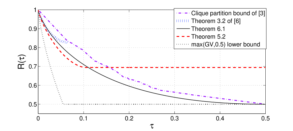
Figure 2. The upper bounds of Theorems 5.2 and 6.1, along with bounds from [3] and [6].

The upper bounds of Theorems 5.2 and 6.1 are plotted in Figure 2. For comparison, also plotted are upper and lower bounds from [3, Figure 1], and the upper bound of Sharov and Roth [6, Theorem 3.2]. The upper bounds from [3] and [6] are the best bounds in the prior literature. Figure 2 clearly shows that the upper bounds of Theorem 5.2 and 6.1 improve upon the previously known upper bounds, but still remain far from the lower bound plotted. It should be pointed that a slightly better lower bound was found by Sharov and Roth [5]. Unfortunately, the improvement is only minor: the lower bound of [5] remains above $0.5$ only in the interval $[0,0.0566]$, and in that interval, the improvement does not exceed $0.012$.

7. Concluding Remarks

In this paper, we derived upper bounds on the maximum cardinality, $M(n,t)$, of a binary $t$-grain-correcting code of blocklength $n$, and also on the asymptotic rate $R(\tau$). In nearly all cases, the gap between the upper bound and the best known lower bound remains significant. A natural question to ask is whether the putative upper bounds on $M(n,t)$ in Conjectures 12 and 16 would yield a better bound on $R(\tau)$.

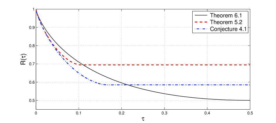
Figure 3. The upper bounds of Theorems 5.2 and 6.1 compared with the asymptotic bound obtained from Conjecture 16.

The bound in Conjecture 16 is the stronger of the two conjectured bounds, and its asymptotics are straightforward to analyze. Let $\overline{M}(n,t)=2\sum_{\omega=0}^{n-1}\binom{n-1}{\omega}\,\frac{1}{V(\omega,t)}$ denote the upper bound in (16), and let $\overline{R}(\tau)=\lim_{n\to\infty}\frac{1}{n}\log_{2}\overline{M}(n,n\tau)$. Conjecture 16 implies that $R(\tau)\leq\overline{R}(\tau)$. By standard asymptotic analysis, we obtain

$$\overline{R}(\tau)=\max_{0\leq\nu\leq 1}[{\mathsf{h}}(\nu)-\eta(\nu)],$$

where $\eta(\nu)$ equals $\nu$ if $\nu\leq 2\tau$, and equals $\nu{\mathsf{h}}(\tau/\nu)$ otherwise. Thus,

$$\overline{R}(\tau)=\max\biggl{\{}\max_{0\leq\nu\leq 2\tau}[{\mathsf{h}}(\nu)-\nu],\,\max_{2\tau\leq\nu\leq 1}[{\mathsf{h}}(\nu)-\nu{\mathsf{h}}(\tau/\nu)]\biggr{\}}.$$

Using elementary calculus to solve the two maximization problems within the braces in the above equation, and comparing the solutions (details of these calculations are omitted), we obtain the following:

$$\overline{R}(\tau)=\begin{cases}{\mathsf{h}}(\nu^{*})-\nu^{*}{\mathsf{h}}(\tau/\nu^{*})&\text{ if }\tau<1/6\\ {\mathsf{h}}(1/3)-1/3&\text{ if }\tau\geq 1/6\end{cases}$$ (31)

where $\nu^{*}=\frac{1}{4}(\tau+1+\sqrt{\tau^{2}-6\tau+1})$. Numerically, ${\mathsf{h}}(1/3)-1/3\approx 0.5850$. This bound is compared with the bounds of Theorem 6.1 in Figure 3. The plot shows that the conjectured upper bound (31) is (expectedly) better than the bound of Theorem 5.2, and improves upon the bound of Theorem 6.1 for $\tau<0.214$.

Appendix A

In this appendix, we prove the following lemma.

Lemma A.1.

For $t=2,3$, a pairing satisfying (13) can be constructed.

We introduce some convenient notation that will be used in the proof. Notation of the form

$$\breve{a}b\longrightarrow cd\ \ \text{ or }\ \ \breve{a}b\stackrel{{\scriptstyle E}}{{\longrightarrow}}cd$$

will be used to denote the fact that a length-2 grain (from the grain pattern $E$) acting on $a$ converts the substring $ab$ of the derivative sequence ${\mathbf{x}}^{\prime}$ to the substring $cd$ of ${\mathbf{y}}^{\prime}$.

Case I: $t=2$.   Let ${\mathbf{y}}\in\Phi_{2}({\mathbf{x}})$. Let $\omega$ and $m$ be the number of $1$-runs and the Hamming weight, respectively, of ${\mathbf{x}}^{\prime}$, and let $\tilde{\omega}$ and $\tilde{m}$ denote the same for ${\mathbf{y}}^{\prime}$. Since the action of a grain pattern cannot increase the weight of ${\mathbf{x}}^{\prime}$, we have $\tilde{\omega}\leq\omega$. Also, note that a single grain can cause the number of $1$-runs in ${\mathbf{x}}^{\prime}$ to increase by a most $1$ — an increase by $1$ happens either when $*1\breve{1}00*\longrightarrow*1010*$, or when $*1\breve{1}11*\longrightarrow*1001*$. Thus, $\tilde{m}\leq m+2$.

We first show that $|\Phi_{2}({\mathbf{y}})|>|\Phi_{2}({\mathbf{x}})|$ iff $\tilde{\omega}=\omega$ and $\tilde{m}>m$. The “if” part is clearly true by Proposition 2.1(b). For the “only if” part, suppose that $\tilde{m}\leq m$. Then, since $\tilde{\omega}\leq\omega$ is always true, we have $|\Phi_{2}({\mathbf{y}})|\leq|\Phi_{2}({\mathbf{x}})|$ by Proposition 2.1(b). On the other hand, if $\tilde{\omega}\leq\omega-1$, then since $\tilde{m}\leq\tilde{\omega}$ is always true (the number of $1$-runs cannot exceed the number of $1$s), we have

$$|\Phi_{2}({\mathbf{y}})|-|\Phi_{2}({\mathbf{x}})|=(\tilde{m}-m)+\binom{\tilde{\omega}}{2}-\binom{\omega}{2}\leq\tilde{\omega}+\binom{\omega-1}{2}-\binom{\omega}{2}=\tilde{\omega}-(\omega-1)\leq 0.$$

Hence, $|\Phi_{2}({\mathbf{y}})|\leq|\Phi_{2}({\mathbf{x}})|$.

Thus, $F_{2}({\mathbf{x}})=\{{\mathbf{y}}\in\Phi_{2}({\mathbf{x}}):\tilde{\omega}=\omega\text{ and }\tilde{m}>m\}$. If ${\mathbf{x}}$ has weight $\omega=1$, then there is no ${\mathbf{y}}\in\Phi_{2}({\mathbf{x}})$ for which $\tilde{m}>m$, so that $F_{2}({\mathbf{x}})=\emptyset$. We henceforth consider $\omega\geq 2$. We assume ${\mathbf{y}}\in F_{2}({\mathbf{x}})$, and suppose that $E\in{\mathcal{E}}_{n,2}$ is a grain pattern such that ${\mathbf{y}}=\phi_{E}({\mathbf{x}})$. Since $\tilde{\omega}=\omega$, the grains in $E$ do not act upon non-trailing $1$s in ${\mathbf{x}}^{\prime}$. Let $\tilde{m}=m+a$, $a=1$ or $2$, so that $|\Phi_{2}({\mathbf{y}})|=|\Phi_{2}({\mathbf{x}})|+a$. We will construct a ${\mathbf{z}}\in G_{2}({\mathbf{x}})$ with which ${\mathbf{y}}$ can be paired.

Suppose first that $a=1$, i.e., $\tilde{m}=m+1$. There is a unique segment $*1100*$ of ${\mathbf{x}}^{\prime}$ such that $*1\breve{1}00*\stackrel{{\scriptstyle E}}{{\longrightarrow}}*1010*$. Let $j$ be the position of the trailing $1$ affected. Consider the grain pattern $E^{\prime}\in{\mathcal{E}}_{n,2}$ that acts instead on the preceding $1$, i.e., the position $j$ in $E$ is replaced by ${j-1}$ in $E^{\prime}$. Let ${\mathbf{z}}=\phi_{E^{\prime}}({\mathbf{x}})$, and note that in ${\mathbf{x}}^{\prime}\stackrel{{\scriptstyle E^{\prime}}}{{\longrightarrow}}{\mathbf{z}}^{\prime}$, the same segment $*1100*$ of ${\mathbf{x}}^{\prime}$ now undergoes the change $*\breve{1}100*\stackrel{{\scriptstyle E^{\prime}}}{{\longrightarrow}}*0000*$. Thus, the number of $1$-runs in ${\mathbf{z}}^{\prime}$ does not exceed the number, $m$, of $1$-runs in ${\mathbf{x}}^{\prime}$; and moreover, $\omega({\mathbf{z}}^{\prime})=\omega-2$. Hence, $|\Phi_{2}({\mathbf{z}})|-|\Phi_{2}({\mathbf{x}})|\leq\binom{\omega-2}{2}-\binom{\omega}{2}=-(2\omega-3)\leq-1$, since we assumed $\omega\geq 2$ at the outset.

Thus, we have $|\Phi_{2}({\mathbf{y}})|=|\Phi_{2}({\mathbf{x}})|+1$ and $|\Phi_{2}({\mathbf{z}})|\leq|\Phi_{2}({\mathbf{x}})|-1$. With this, we have $\frac{1}{|\Phi_{2}({\mathbf{y}})|}+\frac{1}{|\Phi_{2}({\mathbf{z}})|}\geq\frac{2}{|\Phi_{2}({\mathbf{x}})|}$. So, we can pair ${\mathbf{y}}\in F_{2}({\mathbf{x}})$ with ${\mathbf{z}}$.

Now, suppose that $a=2$, i.e., $\tilde{m}=m+2$. There are now exactly two segments of ${\mathbf{x}}^{\prime}$ such that $*1\breve{1}00*\stackrel{{\scriptstyle E}}{{\longrightarrow}}*1010*$. Let $E^{\prime}=E-1$ be obtained by replacing each $j\in E$ by $j-1$, and consider ${\mathbf{z}}=\phi_{E^{\prime}}({\mathbf{x}})$. Once again, the number of $1$-runs in ${\mathbf{z}}^{\prime}$ does not exceed $m$, but now, we have $\omega({\mathbf{z}}^{\prime})=\omega-4$. This time, $|\Phi_{2}({\mathbf{z}})|-|\Phi_{2}({\mathbf{x}})|\leq\binom{\omega-4}{2}-\binom{\omega}{2}=-(4\omega-10)$. Note that $\omega$ must be at least $3$, since $\tilde{m}=m+2$ is not possible when $\omega=2$. Therefore, $|\Phi_{2}({\mathbf{z}})|-|\Phi_{2}({\mathbf{x}})|\leq-4(\omega-10)\leq-2$. Thus, $|\Phi_{2}({\mathbf{y}})|=|\Phi_{2}({\mathbf{x}})|+2$ and $|\Phi_{2}({\mathbf{z}})|\leq|\Phi_{2}({\mathbf{x}})|-2$. Hence, $\frac{1}{|\Phi_{2}({\mathbf{y}})|}+\frac{1}{|\Phi_{2}({\mathbf{z}})|}\geq\frac{2}{|\Phi_{2}({\mathbf{x}})|}$, and we can pair ${\mathbf{y}}$ with this ${\mathbf{z}}$.

By construction, the pairing ${\mathbf{y}}\mapsto{\mathbf{z}}$ is a one-to-one map.

Case II: $t=3$.   Consider any ${\mathbf{y}}\in F_{3}({\mathbf{x}})$. To the notation introduced above, we add $m_{1}$ and $\tilde{m}_{1}$ to denote the number of $1$-runs of length $1$ in ${\mathbf{x}}^{\prime}$ and ${\mathbf{y}}^{\prime}$, respectively. As before, $\tilde{\omega}\leq\omega$, but this time, $\tilde{m}\leq m+3$ since ${\mathbf{x}}^{\prime}$ can be affected by up to three grains. Also, a single grain can cause an increase of $2$ in $m_{1}$: $*01\breve{1}110*\longrightarrow*010010*$ or $*01\breve{1}00*\longrightarrow*01010*$. Hence, $\tilde{m}_{1}\leq m_{1}+6$.

Suppose first that $\tilde{\omega}\leq\omega-2$. Then, from Proposition 2.1(c), we have $|\Phi_{3}({\mathbf{y}})|\leq 1+(m_{1}+6)+(m+3)(\omega-2-3)+2(\binom{\omega-2}{3}+\binom{\omega-2}{2}+2(\omega-2)$. Upon simplifying, we obtain $|\Phi_{3}({\mathbf{y}})|-|\Phi_{3}({\mathbf{x}})|\leq-(\omega^{2}-9\omega+20)-2m$. Since $m\geq 1$, we further obtain $|\Phi_{3}({\mathbf{y}})|-|\Phi_{3}({\mathbf{x}})|\leq-(\omega^{2}-9\omega+22)$, which is a negative quantity. This cannot happen for ${\mathbf{y}}\in F_{3}({\mathbf{x}})$, so $\tilde{\omega}$ must equal $\omega-1$ or $\omega$.

Since $\tilde{\omega}$ equals $\omega-1$ or $\omega$, we may assume that ${\mathbf{y}}=\phi_{E}({\mathbf{x}})$, for some grain pattern $E\in{\mathcal{E}}_{n,3}$ that acts only upon the trailing $1$s in ${\mathbf{x}}^{\prime}$. Let $E_{i}$, $i=1,2,3$ be the subset of $E$ consisting of grains $j$ that act on the trailing $1$s of $1$-runs of length $i$; also let $E_{4}=E\setminus(E_{1}\cup E_{2}\cup E_{3})$ be the subset of $E$ acting on the trailing $1$s of $1$-runs of length at least $4$. Set $e_{i}=|E_{i}|$, $i=1,2,3,4$. It is easy to see that $\tilde{m}\leq m+e_{2}+e_{3}+e_{4}$, while $\tilde{m}_{1}\leq m_{1}+2e_{2}+e_{3}+e_{4}$.

Let $d=e_{2}+e_{3}+e_{4}$. If $d=0$, then $\tilde{m}\leq m$ and $\tilde{m}_{1}\leq m_{1}$. Since $\tilde{\omega}\leq\omega$ always, we have $|\Phi_{3}({\mathbf{y}})|\leq|\Phi_{3}({\mathbf{x}})|$ by Proposition 2.1(c), which is not possible for ${\mathbf{y}}\in F_{3}({\mathbf{x}})$.

At this point, we have that $\tilde{\omega}$ equals $\omega-1$ or $\omega$, and $d$ equals 1, 2, or 3. We will now construct a ${\mathbf{z}}$ to be paired with ${\mathbf{y}}$. Let $E^{\prime}=E_{1}\cup\{j-1:j\in E_{2}\cup E_{3}\cup E_{4}\}$. Thus, $E^{\prime}$ is a grain pattern in ${\mathcal{E}}_{n,3}$ that retains the grains from $E$ that act on trailing $1$s from $1$-runs of length $1$, but pushes back all the other grains in $E$ by one position. Let ${\mathbf{z}}=\phi_{E^{\prime}}({\mathbf{x}})$. We claim that the desired inequality $\frac{1}{|\Phi_{3}({\mathbf{y}})|}+\frac{1}{|\Phi_{3}({\mathbf{z}})|}\geq\frac{2}{|\Phi_{3}({\mathbf{x}})|}$ holds. The remainder of this proof justifies this claim.

It is enough to show that $\frac{1}{2}[|\Phi_{3}({\mathbf{y}})|+|\Phi_{3}({\mathbf{z}})|]\leq|\Phi_{3}({\mathbf{x}})|$, since by the concavity of the function $f(x)=1/x$, we would then have

$$\frac{1}{2}\left[\frac{1}{|\Phi_{3}({\mathbf{y}})|}+\frac{1}{|\Phi_{3}({\mathbf{z}})|}\right]\geq\frac{1}{\frac{1}{2}[|\Phi_{3}({\mathbf{y}})|+|\Phi_{3}({\mathbf{z}})|]}\geq\frac{1}{|\Phi_{3}({\mathbf{x}})|}.$$

To this end, note first that

$$|\Phi_{3}({\mathbf{y}})|-|\Phi_{3}({\mathbf{x}})|\leq 2e_{2}+e_{3}+e_{4}+(\omega-3)d.$$ (32)

Next, we bound $|\Phi_{3}({\mathbf{z}})|-|\Phi_{3}({\mathbf{x}})|$. It is not difficult to check that $\omega({\mathbf{z}}^{\prime})=\omega-2d$, the number of $1$-runs in ${\mathbf{z}}^{\prime}$ is at most $m$, and at most $m_{1}+e_{3}$ of these are of length $1$. Thus, $|\Phi_{3}({\mathbf{z}})|\leq 1+(m_{1}+e_{3})+m(\omega-2d-3)+\binom{\omega-2d}{3}-\binom{\omega-2d}{2}+2(\omega-2d)$, and hence,

$$|\Phi_{3}({\mathbf{z}})|-|\Phi_{3}({\mathbf{x}})|\leq e_{3}-2md-\xi(\omega,d),$$ (33)

where $\xi(\omega,d)=\binom{\omega}{3}-\binom{\omega}{2}+2\omega-\bigl{[}\binom{\omega-2d}{3}-\binom{\omega-2d}{2}+2(\omega-2d)\bigr{]}$. From (32) and (33), we obtain

$$\frac{1}{2}[|\Phi_{3}({\mathbf{y}})|+|\Phi_{3}({\mathbf{z}})|]-|\Phi_{3}({\mathbf{x}})| \leq e_{2}+e_{3}+\frac{1}{2}e_{4}+\frac{1}{2}(\omega-3)d-md-\frac{1}{2}\xi(\omega,d)$$ (34)

$$\leq d+\frac{1}{2}(\omega-3)d-d^{2}-\frac{1}{2}\xi(\omega,d),$$

where we have used the fact that $m\geq d$, which is simply the observation that $|E_{2}\cup E_{3}\cup E_{4}|$ cannot exceed the number of $1$-runs in ${\mathbf{x}}^{\prime}$.

If $d=1$, the expression in (34) reduces to $-\frac{1}{2}(\omega^{2}-7\omega+14)$, a negative quantity. If $d=2$, we obtain $-(\omega^{2}-9\omega+24)$ instead, which is still a negative quantity. If $d=3$, we get $-\frac{3}{2}(\omega^{2}-11\omega+\frac{110}{3})$, which is also a negative quantity. Thus, in all cases, we have $\frac{1}{2}[|\Phi_{3}({\mathbf{y}})|+|\Phi_{3}({\mathbf{z}})|]\leq|\Phi_{3}({\mathbf{x}})|$ as desired. ∎

Appendix B

We prove Theorem 5.2 here. Throughout this appendix, we set $t=\lceil\tau n\rceil$ and $r=\lceil\rho n\rceil$ for some $\tau\in[0,\frac{1}{2}]$ and $\rho\in[0,1]$.

The asymptotics of $\varphi_{n,t}(r)$ is determined by the largest term within the summation in (25). Letting $\zeta_{j}=\binom{r-j}{j}$, it is easy to verify that the ratio $\zeta_{j-1}/\zeta_{j}$ is at most $1$ when $j\leq\frac{1}{10}(5r+7-\sqrt{5r^{2}+10r+9})$, and is strictly larger than $1$ for $\frac{1}{10}(5r+7-\sqrt{5r^{2}+10r+9})<j\leq r/2$; for $j>r/2$, we have $\zeta_{j}=0$. Therefore, setting $J=\lfloor{\frac{1}{10}(5r+7-\sqrt{5r^{2}+10r+9})}\rfloor$, we see that if $t<J$, then the dominant term in (25) is $\zeta_{t}$; and if $t\geq J$, the dominant term is $\zeta_{J}$. Passing to asymptotics, it follows that if we define $\alpha=\frac{5-\sqrt{5}}{10}$, then

$$\lim_{n\to\infty}\frac{1}{n}\log_{2}\varphi_{n,\lceil{\tau n\rceil}}(\lceil\rho n\rceil)=\begin{cases}(\rho-\tau){\mathsf{h}}\left(\frac{\tau}{\rho-\tau}\right)&\text{ if }\tau\leq\alpha\rho\\ \rho(1-\alpha){\mathsf{h}}(\frac{\alpha}{1-\alpha})&\text{ if }\tau\geq\alpha\rho\end{cases}$$ (35)

We record in the following lemma some facts about the constant $\alpha=\frac{5-\sqrt{5}}{10}$ that will be useful in the sequel. They are proved by straightforward algebraic manipulations. For ease of verification, we give a proof of part (c) at the end of this appendix.

Lemma B.1.

Recall that $\phi=\frac{1+\sqrt{5}}{2}$ is the golden ratio.

• $\alpha^{-1}=\sqrt{5}\phi$

• $\frac{\alpha}{1-\alpha}=\frac{1}{1+\phi}$

• $(1-\alpha){\mathsf{h}}(\frac{\alpha}{1-\alpha})=\log_{2}\phi$.

Resuming the proof of Theorem 5.2, from (24), we obtain

$$R(\tau)\leq\max_{0\leq\rho\leq 1}\left[{\mathsf{h}}(\rho)-\lim_{n\to\infty}\frac{1}{n}\varphi_{n,\lceil\tau n\rceil}(\lceil\rho n\rceil)\right].$$

Hence, using (35) and Lemma B.1, we have

$$R(\tau)\leq\max\{A(\tau),B(\tau)\},$$ (36)

where

$$A(\tau)=\max_{0\leq\rho\leq\min\{\alpha^{-1}\tau,1\}}[{\mathsf{h}}(\rho)-\rho\log_{2}\phi],$$ (37)

and

$$B(\tau)=\max_{\alpha^{-1}\tau\leq\rho\leq 1}\left[{\mathsf{h}}(\rho)-(\rho-\tau){\mathsf{h}}\left(\frac{\tau}{\rho-\tau}\right)\right]$$ (38)

For convenience, we define $B(\tau)=0$ if $\alpha^{-1}\tau>1$. Note that the term within square brackets in (38) reduces to ${\mathsf{h}}(\alpha^{-1}\tau)-\alpha^{-1}\tau\log_{2}\phi$ if we set $\rho=\alpha^{-1}\tau$; therefore, ${\mathsf{h}}(\alpha^{-1}\tau)-\alpha^{-1}\tau\log_{2}\phi\leq B(\tau)$.

Now, using elementary calculus to solve the maximization problem in (37), we obtain

$$A(\tau)=\begin{cases}{\mathsf{h}}(\alpha^{-1}\tau)-\alpha^{-1}\tau\log_{2}\phi&\text{ if }\alpha^{-1}\tau\leq\frac{1}{1+\phi}\\ {\mathsf{h}}\left(\frac{1}{1+\phi}\right)-\frac{1}{1+\phi}\cdot\log_{2}\phi&\text{ if }\alpha^{-1}\tau\geq\frac{1}{1+\phi}\end{cases}$$

Somewhat miraculously, the expression ${\mathsf{h}}(\frac{1}{1+\phi})-\frac{1}{1+\phi}\cdot\log_{2}\phi$ simplifies to $\log_{2}\phi$ using parts (b) and (c) of Lemma B.1: replace $\frac{1}{1+\phi}$ and $\log_{2}\phi$ by $\frac{\alpha}{1-\alpha}$ and $(1-\alpha){\mathsf{h}}(\frac{\alpha}{1-\alpha})$, respectively, and simplify. Thus, we have

$$A(\tau)=\begin{cases}{\mathsf{h}}(\alpha^{-1}\tau)-\alpha^{-1}\tau\log_{2}\phi&\text{ if }\alpha^{-1}\tau\leq\frac{1}{1+\phi}\\ \log_{2}\phi&\text{ if }\alpha^{-1}\tau\geq\frac{1}{1+\phi}\end{cases}$$ (39)

As a result, when $\alpha^{-1}\tau\leq\frac{1}{1+\phi}$, we have $A(\tau)={\mathsf{h}}(\alpha^{-1}\tau)-\alpha^{-1}\tau\log_{2}\phi\leq B(\tau)$. Thus, (36) reduces to $R(\tau)\leq B(\tau)$, which proves one half of Theorem 5.2.

To complete the proof of the theorem, we must show that when $\alpha^{-1}\tau\geq\frac{1}{1+\phi}$, we have $A(\tau)\geq B(\tau)$. This would then imply that $\max\{A(\tau),B(\tau)\}=A(\tau)=\log_{2}\phi$ by (39). The above clearly holds when $\alpha^{-1}\tau>1$, since $B(\tau)=0$ in this case; so we henceforth assume $1\geq\alpha^{-1}\tau\geq\frac{1}{1+\phi}$.

We will show that the maximum in the definition of $B(\tau)$ is achieved at $\rho=\alpha^{-1}\tau$. With this, $B(\tau)={\mathsf{h}}(\alpha^{-1}\tau)-\alpha^{-1}\tau\log_{2}\phi\leq{\displaystyle\max_{0\leq\rho\leq\alpha^{-1}\tau}}[{\mathsf{h}}(\rho)-\rho\log_{2}\phi]=A(\tau)$.

Define $f_{\tau}(\rho)={\mathsf{h}}(\rho)-(\rho-\tau){\mathsf{h}}(\frac{\tau}{\rho-\tau})$, so that $B(\tau)=\max_{\alpha^{-1}\tau\leq\rho\leq 1}f_{\tau}(\rho)$. We want to show that, under the assumption $1\geq\alpha^{-1}\tau\geq\frac{1}{1+\phi}$, the function $f_{\tau}(\rho)$ is monotonically decreasing in the range $\alpha^{-1}\tau\leq\rho\leq 1$. We accomplish this by showing that $f_{\tau}^{\prime}(\alpha^{-1}\tau)\leq 0$, and $f^{\prime\prime}_{\tau}(\rho)<0$ for $\alpha^{-1}\tau\leq\rho\leq 1$. Here, all derivatives are with respect to the variable $\rho$.

$f_{\tau}^{\prime}(\alpha^{-1}\tau)\leq 0$: Computing the derivative $f_{\tau}^{\prime}(\rho)$ by direct differentiation, then plugging in $\rho=\alpha^{-1}\tau$ and simplifying using Lemma B.1, we obtain

$$f_{\tau}^{\prime}(\alpha^{-1}\tau)=\log_{2}\frac{1-\alpha^{-1}\tau}{\alpha^{-1}\tau}-\log_{2}\phi=g^{\prime}(\alpha^{-1}\tau),$$

where $g$ is the function defined by $g(x)={\mathsf{h}}(x)-(\log_{2}\phi)x$. Observe that $g(x)$ is strictly concave on $[0,1]$, and attains its unique maximum at $x=\frac{1}{1+\phi}$. Hence, for $x\geq\frac{1}{1+\phi}$, $g^{\prime}(x)\leq 0$. In particular, $g^{\prime}(\alpha^{-1}\tau)\leq 0$.

$f_{\tau}^{\prime\prime}(\rho)<0$ for $\alpha^{-1}\tau\leq\rho\leq 1$: Routine differentiation yields

$$f_{\tau}^{\prime\prime}(\rho)=-\frac{1}{1-\rho}-\frac{1}{\rho}+\frac{\tau}{(\rho-\tau)(\rho-2\tau)}.$$

For $\tau\leq\alpha\rho$, we have

$$\frac{\tau}{(\rho-\tau)(\rho-2\tau)} \ \leq\ \frac{\alpha\rho}{(\rho-\alpha\rho)(\rho-2\alpha\rho)}$$

$$\ =\ \frac{\alpha}{(1-\alpha)(1-2\alpha)}\cdot\frac{1}{\rho}\ =\ \frac{5-\sqrt{5}}{1+\sqrt{5}}\cdot\frac{1}{\rho}\ <\ \frac{1}{\rho}.$$

Hence, $f_{\tau}^{\prime\prime}(\rho)<-\frac{1}{1-\rho}<0$.

This completes the proof of Theorem 5.2, modulo the promised proof of Lemma B.1(c).

Proof of Lemma B.1(c): We first write

$$(1-\alpha){\mathsf{h}}\left(\frac{\alpha}{1-\alpha}\right)=-\alpha\log_{2}(\alpha(1-\alpha))-(1-2\alpha)\log_{2}(1-2\alpha)+\log_{2}(1-\alpha).$$

Using $\alpha(1-\alpha)=\frac{1}{5}$ and $1-2\alpha=\frac{1}{\sqrt{5}}$, the right-hand side above simplifies to

$$\frac{1}{2}\log_{2}5+\log_{2}(1-\alpha)\ =\ \log_{2}[\sqrt{5}(1-\alpha)].$$

It is easy to verify that $\sqrt{5}(1-\alpha)=\phi$. ∎

References

[1] A.A. Kulkarni and N. Kiyavash, “Non-asymptotic upper bounds for deletion correcting codes,”
arXiv:1211.3128, Nov. 2012.
[2]
C. Berge, “Packing Problems and Hypergraph Theory: A Survey,”
Annals of Discrete Mathematics, vol. 4, pp. 3–37, 1979.
[3] A. Mazumdar, A. Barg and N. Kashyap, “Coding for high-density recording on a 1-d granular magnetic medium,” IEEE Trans. Inform. Theory, vol. 57, no. 11, pp. 7403–7417, Nov. 2011.
[4] L. Pan, W.E. Ryan, R. Wood and B. Vasic, “Coding and detection for rectangular grain models,”
IEEE Trans. Magn., vol. 47, no. 6, pp. 1705–1711, June 2011.
[5] A. Sharov and R.M. Roth, “Bounds and constructions for granular media coding,”
Proc. 2011 IEEE Int. Symp. Inform. Theory (ISIT 2011), pp. 2304–2308.
[6] A. Sharov and R.M. Roth, “Bounds and constructions for granular media coding,”
submitted to IEEE Trans. Inform. Theory, 2013.
[7] R. Wood, M. Williams, A. Kavcic and J. Miles, “The feasibility of magnetic recording at
10 Terabits per square inch on conventional media,” IEEE Trans. Magn., vol. 45, no. 2, pp. 917–923, Feb. 2009.