Generation of Electrostatic Waves via Parametric Instability and Heating of Solar Corona

Abstract

Context. In the upper layers of the solar atmosphere the temperature increases sharply. We studied possibility of the transfer of neutrals motion energy into the electrostatic waves.Electrostatic waves could damp in the upper layers of the solar atmosphere and their energy could be transformed into the thermal energy of the solar atmosphere plasma.

Aims. We have used the two fluid approximation when studying plasma dynamics in the low altitudes of the solar atmosphere. In order to study evolution of disturbances of high amplitudes the parametric resonance technique is used.

Methods. The dispersion relation for the electrostatic waves excited due tot he motion of neutrals is derived. The frequencies of electromagnetic waves which could be excited due to existence of the acoustic wave are found. The increment of excited electrostatic waves are determined.

Results. The motion of the neutrals in the lower solar atmosphere, where ionization rate is low, could excite electrostatic waves. In the upper solar atmosphere the ionization rate increases and motion of the neutrals could not support electrostatic waves and these waves could damp due to the collision of the charged particles. The energy of the damping waves could be transformed into the thermal energy of the plasma in the upper atmosphere.

Conclusions.

1 Introduction

In the solar atmosphere the temperature raises sharply from photospheric 6000K to few $10^{6}K$ in the corona. The problem of heating solar atmosphere is a long standing problem in solar Physics. The detailed physical mechanism of coronal heating is not yet well understood, fundamental problems have to be solved in order to find proper theoretical models explaining observational data. Fundamental questions related with the coronal heating include identification of the source of thermal energy, proposition of the energy release mechanism and comparison of theoretically predicted values of the physical characteristics with observations (Klimchuk, 2006). Investigation of the coronal heating needs the study of the highly disparate spatial scales, in particular the study of MHD wave dispassion, MHD reconnection, quasi-periodic oscillations and small-scale bursts occurring in corona is necessary (Klimchuk, 2006, Walsh & Irelan, 2003).In addition, the heating of the chromosphere requires much more energy, and this related process is equally difficult to understand.

Based on the UV and X-ray observations of the sun, Parker suggested (1988) that the X-ray solar corona is created by the dissipation at the many tangential discontinuities arising spontaneously in the bipolar fields of the solar active regions as consequence of random continuous motion of the footpoints of the field in the photospheric convection. Parker named these elementary energy release vents as nanoflares. Number of studies were dedicated to finding observational evidences of nanoflares (Cargill, 1994, Sakamoto et al., 2008, Vekstein, 2009). Prominent researchers found Parkers’s idea very promising and investigated nanoflares contribution into energy budget of the solar corona (Klimchuk, 2006).

Parker’s model does not address following questions: where the excess magnetic energy comes form and what is its original source? According to Rappazzo et al., (2008) slow photospheric motions induce a Poynting flux which saturates by driving an anisotropic turbulent cascade dominated by magnetic energy. In this case magnetic field lines are barely tangential and current sheets are continuously formed and dissipated (current sheets correspond to tangential discontinuities Proposed by Parker).

Another mechanism was suggested by Krasnoselskikh et al., (2010), that electric waves could be generated by motion of neutral gas. A huge energy reservoir exists in the form of turbulent motion of neutral gas at end beneath the photosphere. It is widely accepted that this energy could be partially transformed into the excess magnetic energy in the chromosphere and corona.

The mechanism of transformation of neutral gas motion energy into the electromagnetic disturbances was investigated by Aburjania & Machabeli (1998). In this paper authors derived dispersion equations for coupled acoustic and electromagnetic modes. The authors considered studied parametric instability. This technique enables to study nonlinear processes, i.e. pumping energy from the acoustic waves with high amplitudes. In Aburjania & Machabeli (1998) authors implied discussed mechanism to explain observed data and predict characteristic expected atmospheric wave preprocesses before the earthquakes.

In order to study excitation of the electromagnetic waves in solar atmosphere we use data, describing parameters of solar atmosphere given by Vernaza et al. (1981). We consider the case where excited velocities, electric field and wave vector and are parallel to external magnetic field.

2 Main consideration

In the low layers of the solar atmosphere (up to 1000 km, see Vernaza et al. 1981), the concentration of neutral is much higher than concentration of the charged component of plasma. At this altitudes of the solar atmosphere the motion of neutrals could influence dynamics of electrons and ions, therefore the energy of motion of neutrals could be transformed into the electromagnetic energy, in particular energy of the acoustic waves could be pumped into the energy of the electrostatic waves. The intensive acoustic wave draws charged particles into the motion due to friction with neutrals.

Here we investigate how the energy of acoustic waves with high amplitude, could be transformed into the energy of electrostatic waves. When considering the disturbances of high amplitudes, we could not neglect nonlinear terms, more over these terms play a key role in the process. The nonlinear pumping of the electromagnetic wave energy into the plasma, due to the parametric instability was studied by Silin (1973), in order to investigate neutral wave energy pumping into the plasma the parametric instability mechanism was studied by Aburjania Machabeli (1998), in this work we also apply parametric instability technique.

If we write and sum the equations of motion for electrons and ions,

we will get:

$$m_{e}n_{e}\frac{d\upsilon_{e}}{dt}+m_{i}n_{i}\frac{d\upsilon_{i}}{dt}=$$

$$-\nabla\left(p_{e}+p_{i}\right)-m_{i}n_{i}\nu_{in}\left(\upsilon_{i}-\upsilon_{n}\right)+m_{i}n_{i}\nu_{ie}\left(\upsilon_{e}-\upsilon_{i}\right)$$

$$+m_{e}n_{e}\nu_{ei}\left(\upsilon_{i}-\upsilon_{e}\right)+m_{e}n_{e}\nu_{en}\left(\upsilon_{n}-\upsilon_{e}\right).$$

Here is assumed that charged particle move along the magnetic field lines ant the direction of electric field and wave vector coincides with the direction of the magnetic field, i.e we consider electrostatic waves.

In the low altitude (beyond 1000km) of the solar atmosphere the relations given below by Eq. 2a-2d are satisfied:

$$\frac{\nu_{en}}{\nu_{in}}=\sqrt{\frac{m_{i}}{m_{e}}},$$

$$\frac{\nu_{ei}}{\nu_{ie}}=\sqrt{\frac{m_{i}}{m_{e}}},$$

$$\frac{\nu_{in}}{\nu_{ni}}\approx\frac{n_{0n}}{n_{0i}}\gg 1,$$

If the electric field changes with frequency much less than the cyclotron frequency we could assume that the charged particle moves in a constant electric field during the Larmour rotation period. In this case the velocity of the charged particle is: $\upsilon_{\alpha z}=q_{\alpha}\frac{E_{z}}{m_{\alpha}}t$ (here indices $\alpha$ shows the sort of particle and $t$ is time). In order to define the interval between collisions of the charged particle kind $\alpha$ with neutrals we use the law of statistical distribution (see Aburjania & Machabeli 1998), i.e the probability that collision of particle $\alpha$ with neutrals happens between $t$ and $t+dt$ is: $f_{\alpha n}=\nu_{\alpha n}e^{-\nu_{\alpha n}t}dt.$ Multiplication of $\upsilon_{\alpha z}=q_{\alpha}\frac{E_{z}}{m_{\alpha}}t$ by $f_{\alpha n}=\nu_{\alpha n}e^{-\nu_{\alpha n}t}dt$ and integration by time leads to the following relation between velocities of electron and ions:

$$\upsilon_{ez}=-\beta\upsilon_{iz},$$

here:

$\beta=\frac{m_{i}\nu_{in}}{m_{e}\nu_{en}}.$ Eq. 2d helps us to solve us three component hydrodynamic equations system.

After taking into account relations given by Eq. 2a-2d and comparing similar terms in Eq. (1), we obtain:

$$\frac{m_{i}n_{i}}{m_{e}n_{e}}\frac{d\upsilon_{i}/dt}{d\upsilon_{e}/dt}\approx\frac{n_{i}\omega_{pi}}{n_{e}\omega_{pe}}\approx\sqrt{\frac{m_{i}}{m_{e}}}\gg 1,$$

$$\frac{m_{i}n_{i}\nu_{in}}{m_{e}n_{e}\nu_{en}}=\sqrt{\frac{m_{i}}{m_{e}}}\gg 1,$$

$$\frac{m_{i}n_{i}\nu_{ie}(\upsilon_{e}-\upsilon_{i})}{m_{e}n_{e}\nu_{ei}(\upsilon_{e}-\upsilon_{i})}=\sqrt{\frac{m_{i}}{m_{e}}}\gg 1,$$

$$\upsilon_{e}\gg\upsilon_{i}.$$

After taking into account Eq. (3a-3d) and neglecting electron inertia, we could rewrite Eq. 1 as follows:

$$\frac{\partial\upsilon_{i}}{\partial t}+\left(\nabla\upsilon_{i}\right)\upsilon_{i}=$$

$$-\frac{1}{m_{i}n_{i}}\nabla\left(p_{e}+p_{i}\right)-\nu_{in}\left(\upsilon_{i}-\upsilon_{n}\right)+\nu_{ie}\left(\upsilon_{e}-\upsilon_{i}\right).$$

If we represent ion velocity as:

$$\upsilon_{i}-\upsilon_{n}=-V_{i},$$

we express the velocity of neutrals as follows:

$$\upsilon_{n}=V_{0}\cos(\Omega t+\Psi),$$

Eq. 5b describes oscillatory motion of the neutrals, this type of motion accompanies the excitation and propagation of waves interacting with neutrals. In Eq. 5b $\Psi$ is casual, initial phase of neutrals oscillations. Because of the collisions between particles the phase of the oscillations changes casually, the final expressions of the variables obtained after solving hydrodynamic equations should be averaged by $\Psi$.

After substitution of (5a-5b) in Eq. (4) we get

$$\frac{\partial V_{i}}{\partial t}-V_{0}\Omega\sin(\Omega t+\Psi)+ikV_{i}V_{0}\cos(\Omega t+\Psi)=$$

$$-\frac{1}{m_{i}n_{i}}\nabla\left(p_{e}+p_{i}\right)-V_{i}\left(\nu_{in}+\beta\nu_{ie}\right)-\nu_{ie}\beta V_{0}\cos(\Omega t+\Psi),$$

and

$$\frac{\partial V_{i}}{\partial t}-V_{0}\left[\Omega\sin(\Omega t+\Psi)+\nu_{ei}\cos(\Omega t+\Psi)\right]+ikV_{i}V_{0}\cos(\Omega t+\Psi)=$$

$$-\frac{1}{m_{i}n_{i}}\nabla\left(p_{e}+p_{i}\right)-V_{i}\left(\nu_{in}+\nu_{ei}\right).$$

It is convenient to use notation:

$$V_{i}\equiv U\exp\left[ia\sin(\Omega t+\Psi)\right].$$

Substitution of Eq. (7) into Eq. (6b) leads to equation:

$$\frac{\partial U}{\partial t}-V_{0}\left[\Omega\sin(\Omega t+\Psi)+\nu_{ei}\cos(\Omega t+\Psi)\right]\exp\left[-ia\sin(\Omega t+\Psi)\right]=$$

$$-\frac{1}{m_{i}n_{i}}\nabla\left(p_{e}+p_{i}\right)\exp\left[-ia\sin(\Omega t+\Psi)\right]-U\left(\nu_{in}+\nu_{ei}\right).$$

Let us write equation of continuity:

$$\frac{\partial{(n_{0}+n_{e})}}{\partial t}+\nabla(n_{0}+n_{e})\mathbf{\upsilon_{e}}=0,$$

unperturbed value of concentration-$n_{0}$ does not depend on time, therefore $\frac{\partial n_{0}}{\partial t}=0.$ It is convenient to introduce notation $n_{e}=N_{e}(t)\exp\left[-ib\sin(\Omega t+\Psi)\right],$ here $a=\frac{kV_{0}}{\Omega},b=\beta\frac{kV_{0}}{\Omega},\beta=\sqrt{\frac{m_{i}}{m_{e}}}.$ For $N_{e}$ we get equation:

$$\frac{\partial N_{e}}{\partial t}-ik\beta U(t)n_{0}\exp\left[-ib\sin(\Omega t+\Psi)+ia\sin(\Omega t+\Psi)\right],$$

solution of Eq. 9b gives

$$n_{e}=ikn_{0}\beta\exp[ib\sin(\Omega t+\Psi)]\times$$

$$\times\sum J_{\eta}(b)\exp(i\eta\Psi)\int\frac{U(\omega^{\prime})\exp\left[-i(\omega^{\prime}+\eta\Omega)\right]}{\omega^{\prime}+\eta\Omega}d\omega^{\prime}.$$

For pressure gradients we have:

$$\frac{1}{m_{i}n_{0}}\nabla p_{i}=\frac{k^{2}V_{Ti}^{2}}{\omega},$$

$$\frac{1}{m_{i}n_{0}}\nabla p_{e}=\frac{-ikT_{e}n_{e}}{m_{i}n_{0}},$$

here $V_{Ti}=\sqrt{\frac{\gamma kT_{i}}{m_{i}}}.$

After substitution of expressions (9c), (10a), (10b) into equation (8) and averaging by $\Psi$ (it is casual phase of neutrals oscillations) we could derive equation for frequency of excited electrostatic waves:

$$\omega^{2}+i\nu\omega-k^{2}V_{Ti}^{2}-\beta(kV_{se})^{2}\omega\sum{\frac{J_{j_{0}}^{2}(b)}{\omega-j_{0}\Omega}}=0,$$

where:

$\nu=\nu_{in}+\nu_{ei},$ $\omega_{0}=j_{0}\Omega,$

$V_{se}=\sqrt{\frac{\gamma kT_{e}}{m_{i}}}.$

For $\nu_{in}$ and $\nu_{ei}$ the expressions given in Braginskii (1963) are used.

Because of the nonlinear character of the investigated processes, the averaging by casual phase $\Psi$, the terms of hydrodynamic equations, which depend on $\Psi$ do not vanish.

In Eq. 9 we see that resonance occurs when $\omega\approx j_{0}\Omega$. It is convenient to represent $\omega$ in the following way:

$$\omega=\omega_{0}+i\delta.$$

here $\omega_{0}=j_{0}\Omega$

after substitution of Eq. 12 into Eq. 11 we obtain expression for frequency of the excited wave and their increment:

$$\omega_{0}=\pm\sqrt{\delta\nu+k^{2}V_{Ti}^{2}+J_{j_{0}}^{2}(b)\beta(kV_{se})^{2}},$$

$$\delta=-\frac{\nu}{4}\pm\sqrt{\frac{\nu^{2}}{16}+0.5J_{j_{0}}^{2}(b)\beta(kV_{se})^{2}},$$

We could solve equations 13a and 13b numerically. Fig. 1 shows values of the function $f_{\omega}(k,j_{0})$, where $f_{\omega}(k,j_{0})=\omega$ if the Eqs.13a-b have solution and $f_{\omega}(k,j_{0})=0$ if Eqs.13a-b do not have solutions. Fig. 2 represents values of the function $f_{\delta}(k,j_{0})$, where $f_{\delta}(k,j_{0})=\delta$ if the Eqs.13a-b have solution and $f_{\delta}(k,j_{0})=0$ if Eqs.13a-b do not have solutions. When solving equations the parameters, given in paper by Vernazza et al. (1981), are used.

In our model the only source of excitation of electrostatic waves is the oscillation of neutrals, in the case of absence of acoustic waves i.e. $V_{0}=0$, in the fourth term of Eq. 11 $\sum{\frac{J_{j_{0}}^{2}(b)}{\omega-j_{0}\Omega}}=\frac{J_{0}(0)}{\omega}=\frac{1}{\omega}$, therefore we have:

$$\omega^{2}+i\nu_{ei}\omega-k^{2}V_{Ti}^{2}-\beta(kV_{se})^{2}=0,$$

the solution of Eq. 14 is:

$$\omega=-\frac{i\nu_{ei}}{2}\pm\sqrt{\frac{\nu_{ei}^{2}}{4}+k^{2}V_{Ti}^{2}+\beta(kV_{se})^{2}}.$$

Eq. 15 represent the damping wave with decrement $\frac{\nu_{ei}}{2}$ and dispersion relation $\omega_{0}=\pm\sqrt{\frac{\nu_{ei}^{2}}{4}+k^{2}V_{Ti}^{2}+\beta(kV_{se})^{2}}$, this result shows the fact that in the absence of acoustic waves the electrostatic waves could not be excited and where the motion of the neutrals does not play a role the damping of propagating electrostatic waves will occur.

In the regions of the solar atmosphere where the plasma ionization rate is high the motion of the neutrals does not influence the dynamics of the charged particles. Due to collisions between the charged particles the damping of the electrostatic wave will occur and the energy of electrostatic waves could be transformed into the thermal energy of the solar atmosphere. The Fig. 3 shows dependence of the collision frequencies $\nu_{ei}$ and $\nu_{en}$ on the altitude in the solar corona, we see that at high altitudes $\nu_{ei}$ (which is responsible for wave damping) is higher than $\nu_{en}$. For the Fig. 3 the solar atmosphere model given by Vernazza et al. (1981) is used. The dependence of the characteristic frequencies on the altitude in the solar atmosphere is given in Krasnoselskikh et al. (2010), where the model of the sun described in Fontenla et al. (2009) is used.

3 Conclusions

We investigated possibility of transformation of neutral gas motion energy into the electromagnetic energy, in the solar atmosphere. We described pumping of the acoustic wave energy into the energy of electrostatic waves in the regions of the solar atmosphere where concentration of the neutrals is much higher than concentration of the charged particles.

With increasing of the height in the solar atmosphere the ionization rate of the plasma increases i.e the role of the motion of the neutrals in the process of wave generation decreases and waves damp due tot he collision of the charged particles. The energy of the damping waves could be transferred in to the thermal energy of the solar atmosphere plasma, at higher altitudes the temperature of the solar atmosphere plasma increases (Vernazza et al. 1981).

We used two fluid approach and the parametric instability technique is used. We have determined that for particular parameters anergy of acoustic waves of certain frequencies and certain wavelength could be pumped into the energy of the electrostatic waves. Figs 1 and 2 what kind of acoustic waves could contribute into the growth of the electrostatic waves.

In this paper the problem was investigated using two fluid MHD approximation, we find it interesting to study transformation of neutral gas energy into the electromagnetic energy using kinetic approach, these approach could lead to more precise results.

4 Acknowledgments

G.Machabeli would like to thank A.S. Volokitin for interesting discussions and he is grateful to LPC2E, CNRS-University of Orl eans for support of his research.

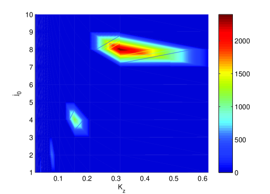
Figure 1: Dependence of ”filtered”, excited waves frequency on wave number and $j_{0}$. Following particular parameters are chosen: $n_{0n}=10^{21}\rm{m^{-3}},$ $T=4070K$.

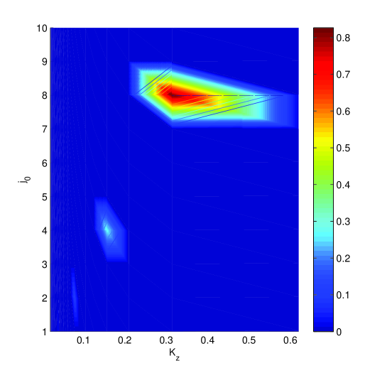
Figure 2: Dependence of excited waves ”filtered” increment on wave number and $j_{0}$. Following particular parameters are chosen: $n_{0n}=10^{21}\rm{m^{-3}},$ $T=4070K$.

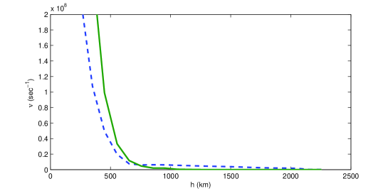
Figure 3: Dependence of the collision frequencies $\nu_{ie}$-dashed line and $\nu_{en}$-solid line, on the altitude in the solar atmosphere.

References

- aburjaniamachabeli (1998) Aburjania, G., Machabeli, G., 1998, J. Geophys. Res., 103, 9441
- braginskii (1963) Braginskii, S. L., The phenomenon of transpher in plasma, 1963, Atomizdat, Moscow
- WalshIreland (2003) walshireland03) Walsh, R. E.,Ireland, J., 2003, A%A. Rev., 12, 1
- Cargill (1994) cargill94) Cargill, P. J., 1994, ApJ, 422, 381
- Fontenla (2009) Fontenla, J. M., Curdt, W., Habbereiter, M., Harder J., Tian, H., 2009, ApJ, 7070, 482
- Klimchuk (2006) klimchuk06) Klimchuk, J. A., 2006, Sol.Phys., 234, 41
- kranoselskikh et al. (2010) Krasnoselskikh, V., Vekstein, G., Hudson, H. S., Bale, S. D., Abbett, W. P., 2010, ApJ, 724, 1542
- Parker (1988) parker08) Parker, E. N., 1988, APJ, 330, 474
- Rappazzo (2008) rappazo08) Rappazzo, A. F., Velli, M., Einaudi, G., Dalburg, R. B., 2008, ApJ, 677, 1348
- Sakamoto (2008) sakamoto08) Sakamoto, Y., Tsuneta, S., Vekstein, G., 2008, APJ, 689, 1421
- silin (1973) Silin, V. P., Parametric Influence High-Intensity Radiation Upon Plasma, 1973, Nauka, Moscow
- Vekstein (2009) vekstein09) Vekstein, G., 2009, A$A, 499, L5
- vernazza (1981) Vernazza, J. E., Avrett, E. H., Loeser, R., 1981, ApJs, 45, 635