Designing Unimodular Codes via Quadratic Optimization is not Always Hard

Abstract

The NP-hard problem of optimizing a quadratic form over the unimodular vector set arises in radar code design scenarios as well as other active sensing and communication applications. To tackle this problem (which we call unimodular quadratic programming (UQP)), several computational approaches are devised and studied. A specialized local optimization scheme for UQP is introduced and shown to yield superior results compared to general local optimization methods. Furthermore, a monotonically error-bound improving technique (MERIT) is proposed to obtain the global optimum or a local optimum of UQP with good sub-optimality guarantees. The provided sub-optimality guarantees are case-dependent and generally outperform the $\pi/4$ approximation guarantee of semi-definite relaxation. Several numerical examples are presented to illustrate the performance of the proposed method. The examples show that for cases including several matrix structures used in radar code design, MERIT can solve UQP efficiently in the sense of sub-optimality guarantee and computational time.

I Introduction

Unimodular codes are used in many active sensing and communication systems mainly as a result of the their optimal (i.e. unity) peak-to-average-power ratio (PAR). The design of such codes can be often formulated as the optimization of a quadratic form (see sub-section I-A for examples). Therefore, we will study the problem

$$\mbox{UQP: }~{}\max_{{\boldsymbol{s}}\in\Omega^{n}}{\boldsymbol{s}}^{H}{\boldsymbol{R}}{\boldsymbol{s}}$$ (1)

where ${\boldsymbol{R}}\in{\mathbb{C}}^{n\times n}$ is a given Hermitian matrix, $(.)^{H}$ denotes the vector/matrix Hermitian transpose, $\Omega$ represents the unit circle, i.e. $\Omega=\{s\in{\mathbb{C}}:~{}|s|=1\}$ and UQP stands for Unimodular Quadratic Program(ming).

I-A Motivating Applications

To motivate the UQP formulation considered above, we present four scenarios in which a design problem in active sensing or communication boils down to an UQP.

$\bullet$  Designing codes that optimize the SNR or the CRLB: We consider a monostatic radar which transmits a linearly encoded burst of pulses. The observed backscattered signal ${\boldsymbol{v}}$ can be written as (see, e.g. [1]):

$${\boldsymbol{v}}=a({\boldsymbol{c}}\odot{\boldsymbol{p}})+{\boldsymbol{w}},$$ (2)

where $a$ represents both channel propagation and backscattering effects, ${\boldsymbol{w}}$ is the disturbance/noise component, ${\boldsymbol{c}}$ is the unimodular vector containing the code elements, ${\boldsymbol{p}}=(1,e^{j2\pi f_{d}T_{r}},\cdots,e^{j2\pi(n-1)f_{d}T_{r}})^{T}$ is the temporal steering vector with $f_{d}$ and $T_{r}$ being the target Doppler frequency and pulse repetition time, respectively, and the symbol $\odot$ stands for the Hadamard (element-wise) product of matrices.

Under the assumption that ${\boldsymbol{w}}$ is a zero-mean complex-valued circular Gaussian vector with known positive definite covariance matrix $\mathbb{E}[{\boldsymbol{w}}{\boldsymbol{w}}^{H}]={\boldsymbol{M}}$, the signal-to-noise ratio (SNR) is given by [2]

$$\mbox{SNR}=|a|^{2}{\boldsymbol{c}}^{H}{\boldsymbol{R}}{\boldsymbol{c}}$$ (3)

where ${\boldsymbol{R}}={\boldsymbol{M}}^{-1}\odot({\boldsymbol{p}}{\boldsymbol{p}}^{H})^{*}$ with $(.)^{*}$ denoting the vector/matrix complex conjugate. Therefore, the problem of designing codes optimizing the SNR of the radar system can be formulated directly as an UQP. Additionally, the Cramer-Rao lower bound (CRLB) for the target Doppler frequency estimation (which yields a lower bound on the variance of any unbiased target Doppler frequency estimator) is given by [2]

CRLB $$= \left(2|a|^{2}({\boldsymbol{c}}\odot{\boldsymbol{p}}\odot{\boldsymbol{u}})^{H}{\boldsymbol{M}}^{-1}({\boldsymbol{c}}\odot{\boldsymbol{p}}\odot{\boldsymbol{u}})\right)^{-1}$$

$$= \left(2|a|^{2}{\boldsymbol{c}}^{H}{\boldsymbol{R}}^{\prime}{\boldsymbol{c}}\right)^{-1}$$

where ${\boldsymbol{u}}=(0,j2\pi T_{r},\cdots,j2\pi(n-1)T_{r})^{T}$ and ${\boldsymbol{R}}^{\prime}={\boldsymbol{M}}^{-1}\odot({\boldsymbol{p}}{\boldsymbol{p}}^{H})^{*}\odot({\boldsymbol{u}}{\boldsymbol{u}}^{H})^{*}$. Therefore the minimization of CRLB can also be formulated as an UQP. For the simultaneous optimization of SNR and CRLB see [2].

$\bullet$  Synthesizing cross ambiguity functions (CAFs): The ambiguity function (which is widely used in active sensing applications [3][4]) represents the two-dimensional response of the matched filter to a signal with time delay $\tau$ and Doppler frequency shift $f$. The more general concept of cross ambiguity function occurs when the match filter is replaced by a mismatched filter. The cross ambiguity function (CAF) is defined as

$$\chi(\tau,f)=\int_{-\infty}^{\infty}u(t)v^{*}(t+\tau)e^{j2\pi ft}dt$$ (5)

where $u(t)$ and $v(t)$ are the transmit signal and the receiver filter, respectively (the ambiguity function is obtained from (5) with $v(t)=u(t)$). In several applications $u(t)$ and $v(t)$ are given by:

$$u(t)=\sum_{k=1}^{n}x_{k}p_{k}(t),~{}~{}~{}v(t)=\sum_{k=1}^{n}y_{k}p_{k}(t)$$ (6)

where $\{p_{k}(t)\}$ are pulse-shaping functions (with the rectangular pulse as a common example), and

$${\boldsymbol{x}}=(x_{1}\cdots x_{n})^{T},~{}~{}{\boldsymbol{y}}=(y_{1}\cdots y_{n})^{T}$$ (7)

are the code and, respectively, the filter vectors. The design problem of synthesizing a desired CAF has a small number of free variables (i.e. the entries of the vectors ${\boldsymbol{x}}$ and ${\boldsymbol{y}}$) compared to the large number of constraints arising from two-dimensional matching criteria (to a given $|\chi(\tau,f)|$). Therefore, the problem is generally considered to be difficult and there are not many methods to synthesize a desired (cross) ambiguity function. Below, we describe briefly the cyclic approach of [5] for CAF design.

The problem of matching a desired $|\chi(\tau,f)|=d(\tau,f)$ can be formulated as the minimization of the criterion [5]

$$g({\boldsymbol{x}},{\boldsymbol{y}},\phi)=\int_{-\infty}^{\infty}\int_{-\infty}^{\infty}w(\tau,f)\left|d(\tau,f)e^{j\phi(\tau,f)}-{\boldsymbol{y}}^{H}{\boldsymbol{J}}(\tau,f){\boldsymbol{x}}\right|^{2}\ d\tau df$$ (8)

where ${\boldsymbol{J}}(\tau,f)\in{\mathbb{C}}^{n\times n}$ is given, $w(\tau,f)$ is a weighting function that specifies the CAF area which needs to be emphasized and $\phi(\tau,f)$ represent auxiliary phase variables. It is not difficult to see that for fixed ${\boldsymbol{x}}$ and ${\boldsymbol{y}}$, the minimizer $\phi(\tau,f)$ is given by $\phi(\tau,f)=\arg\{{\boldsymbol{y}}^{H}{\boldsymbol{J}}(\tau,f){\boldsymbol{x}}\}$. For fixed $\phi(\tau,f)$ and ${\boldsymbol{x}}$, the criterion $g$ can be written as

$$g({\boldsymbol{y}}) = {\boldsymbol{y}}^{H}{\boldsymbol{D}}_{1}{\boldsymbol{y}}-{\boldsymbol{y}}^{H}{\boldsymbol{B}}^{H}{\boldsymbol{x}}-{\boldsymbol{x}}^{H}{\boldsymbol{B}}{\boldsymbol{y}}+\mbox{const}_{1}$$

$$= ({\boldsymbol{y}}-{\boldsymbol{D}}_{1}^{-1}{\boldsymbol{B}}^{H}{\boldsymbol{x}})^{H}{\boldsymbol{D}}_{1}({\boldsymbol{y}}-{\boldsymbol{D}}_{1}^{-1}{\boldsymbol{B}}^{H}{\boldsymbol{x}})+\mbox{const}_{2}$$

where ${\boldsymbol{B}}$ and ${\boldsymbol{D}}_{1}$ are given matrices in ${\mathbb{C}}^{n\times n}$ [5]. Due to practical considerations, the transmit coefficients $\{x_{k}\}$ must have low PAR values. However, the receiver coefficients $\{y_{k}\}$ need not be constrained in such a way. Therefore, the minimizer ${\boldsymbol{y}}$ of $g({\boldsymbol{y}})$ is given by ${\boldsymbol{y}}={\boldsymbol{D}}_{1}^{-1}{\boldsymbol{B}}^{H}{\boldsymbol{x}}$. Similarly, for fixed $\phi(\tau,f)$ and ${\boldsymbol{y}}$, the criterion $g$ can be written as

$$g({\boldsymbol{x}})={\boldsymbol{x}}^{H}{\boldsymbol{D}}_{2}{\boldsymbol{x}}-{\boldsymbol{x}}^{H}{\boldsymbol{B}}{\boldsymbol{y}}-{\boldsymbol{y}}^{H}{\boldsymbol{B}}^{H}{\boldsymbol{x}}+\mbox{const}_{3}$$ (10)

where ${\boldsymbol{D}}_{2}\in{\mathbb{C}}^{n\times n}$ is given [5]. If a unimodular code vector ${\boldsymbol{x}}$ is desired then the optimization of $g({\boldsymbol{x}})$ is an UQP as $g({\boldsymbol{x}})$ can be written as

$$g({\boldsymbol{x}})=\left(\begin{array}[]{c}e^{j\varphi}{\boldsymbol{x}}\\ e^{j\varphi}\\ \end{array}\right)^{H}\left(\begin{array}[]{cc}{\boldsymbol{D}}_{2}&-{\boldsymbol{B}}{\boldsymbol{y}}\\ -({\boldsymbol{B}}{\boldsymbol{y}})^{H}&0\\ \end{array}\right)\left(\begin{array}[]{c}e^{j\varphi}{\boldsymbol{x}}\\ e^{j\varphi}\\ \end{array}\right)+\mbox{const}_{3}$$ (17)

where $\varphi\in[0,2\pi)$ is a free phase variable.

$\bullet$  Steering vector estimation in adaptive beamforming: Consider a linear array with $n$ antennas. The output of the array at time instant $k$ can be expressed as [6]

$${\boldsymbol{x}}_{k}=s_{k}{\boldsymbol{a}}+{\boldsymbol{n}}_{k}$$ (18)

with $\{s_{k}\}$ being the signal waveform, ${\boldsymbol{a}}$ the associated steering vector (with $|[{\boldsymbol{a}}]_{l}|=1$, $1\leq l\leq n$), and ${\boldsymbol{n}}_{k}$ the vector accounting for all independent interferences.

The true steering vector is usually unknown in practice, and it can therefore be considered as an unimodular vector to be determined [7]. Define the sample covariance matrix of $\{{\boldsymbol{x}}_{k}\}$ as $\widehat{{\boldsymbol{R}}}=\frac{1}{T}\sum_{k=1}^{T}{\boldsymbol{x}}_{k}{\boldsymbol{x}}^{H}_{k}$ where $T$ is the number of training data samples. Assuming some prior knowledge on ${\boldsymbol{a}}$ (which can be represented by $\arg({\boldsymbol{a}})$ being in a given sector $\Theta$), the problem of estimating the steering vector can be formulated as [8]

$$\min_{{\boldsymbol{a}}}~{}~{}{\boldsymbol{a}}^{H}\widehat{{\boldsymbol{R}}}^{-1}{\boldsymbol{a}}~{}$$ (19)

$$\mbox{s.t. }\arg({\boldsymbol{a}})\in\Theta,$$

hence an UQP-type problem. Such problems can be tackled using general local optimization techniques or the optimization scheme introduced in Section III.

$\bullet$  Maximum likelihood (ML) detection of unimodular codes: Assume the linear model

$${\boldsymbol{y}}={\boldsymbol{Q}}{\boldsymbol{s}}+{\boldsymbol{n}}$$ (20)

where ${\boldsymbol{Q}}$ represents a multiple-input multiple-output (MIMO) channel, ${\boldsymbol{y}}$ is the received signal, ${\boldsymbol{n}}$ is the additive white Gaussian noise and ${\boldsymbol{s}}$ contains the unimodular symbols which are to be estimated. The ML detection of ${\boldsymbol{s}}$ may be stated as

$$\widehat{{\boldsymbol{s}}}_{ML}=\arg\min_{{\boldsymbol{s}}\in\Omega^{n}}\|{\boldsymbol{y}}-{\boldsymbol{Q}}{\boldsymbol{s}}\|_{2}$$ (21)

It is straightforward to verify that the above optimization problem is equivalent to the UQP [9]:

$$\min_{\overline{{\boldsymbol{s}}}\in\Omega^{n+1}}~{}\overline{{\boldsymbol{s}}}^{H}{\boldsymbol{R}}\overline{{\boldsymbol{s}}}$$ (22)

where

$${\boldsymbol{R}}=\left(\begin{array}[]{cc}{\boldsymbol{Q}}^{H}{\boldsymbol{Q}}&-{\boldsymbol{Q}}^{H}{\boldsymbol{y}}\\ -{\boldsymbol{y}}^{H}{\boldsymbol{Q}}&0\\ \end{array}\right)\mbox{, }\overline{{\boldsymbol{s}}}=\left(\begin{array}[]{c}e^{j\varphi}{\boldsymbol{s}}\\ e^{j\varphi}\\ \end{array}\right)$$ (27)

and $\varphi\in[0,2\pi)$ is a free phase variable.

I-B Related Work

In [10], the NP-hardness of UQP is proven by employing a reduction from an NP-complete matrix partitioning problem. The UQP in (1) is often studied along with the following (still NP-hard) related problem in which the decision variables are discrete:

$$\mbox{$m$-UQP:}~{}\max_{{\boldsymbol{s}}\in\Omega^{n}_{m}}{\boldsymbol{s}}^{H}{\boldsymbol{R}}{\boldsymbol{s}}$$ (28)

where $\Omega_{m}=\{1,e^{j\frac{2\pi}{m}},\cdots,e^{j\frac{2\pi}{m}(m-1)}\}$. Note that the latter problem coincides with the UQP in (1) as $m\rightarrow\infty$. The authors of [11] show that when the matrix ${\boldsymbol{R}}$ is rank-deficient (more precisely, when $d=$rank$({\boldsymbol{R}})$ behaves like $\mathcal{O}(1)$ with respect to the problem dimension) the $m$-UQP problem can be solved in polynomial-time and they propose a $\mathcal{O}((mn/2)^{2d})$-complexity algorithm to solve (28). However, such algorithms are not applicable to the UQP which corresponds to an infinite $m$.

Studies on polynomial-time algorithms for UQP (and $m$-UQP) have been extensive (e.g. see [9]-[19] and the references therein). In particular, the semi-definite relaxation (SDR) technique has been one of the most appealing approaches to the researchers. To derive an SDR, we note that ${\boldsymbol{s}}^{H}{\boldsymbol{R}}{\boldsymbol{s}}=\mbox{tr}({\boldsymbol{s}}^{H}{\boldsymbol{R}}{\boldsymbol{s}})=\mbox{tr}({\boldsymbol{R}}{\boldsymbol{s}}{\boldsymbol{s}}^{H})$. Hence, the UQP can be rewritten as

$$\max_{{\boldsymbol{S}}}\,\mbox{tr}({\boldsymbol{R}}{\boldsymbol{S}})~{}~{}~{}~{}~{}~{}~{}$$ (29)

$$\mbox{s.t. }{\boldsymbol{S}}={\boldsymbol{s}}{\boldsymbol{s}}^{H},~{}{\boldsymbol{s}}\in\Omega^{n}.$$

If we relax (29) by removing the rank constraint on ${\boldsymbol{S}}$ and the unimodularity constraint on ${\boldsymbol{s}}$ then the result is a semi-definite program:

$$\mbox{SDP: }~{}\max_{{\boldsymbol{S}}}\mbox{tr}({\boldsymbol{R}}{\boldsymbol{S}})~{}~{}~{}~{}~{}~{}~{}$$ (30)

$$\mbox{s.t. }[{\boldsymbol{S}}]_{k,k}=1,~{}~{}1\leq k\leq n,~{}~{}~{}$$

$$~{}~{}~{}~{}~{}~{}{\boldsymbol{S}}\mbox{ is positive semi-definite.}$$

The above SDP can be solved in polynomial time using interior-point methods [15]. The approximation of the UQP solution based on the SDP solution can be accomplished in several ways. For example, we can approximate the phase values of the solution ${\boldsymbol{s}}$ using a rank-one approximation of ${\boldsymbol{S}}$. A more effective approach for guessing ${\boldsymbol{s}}$ is based on randomized approximations (see [10], [16] and [17]). A detailed guideline for randomized approximation of the UQP solution can be found in [17]. In addition, we refer the interested reader to the survey of the rich literature on SDR in [18].

Analytical assessments of the quality of the UQP solutions obtained by SDR and randomized approximation are available. Let $v_{SDR}$ be the expected value of the UQP objective at the obtained randomized solution. Let $v_{opt}$ represent the optimal value of the UQP objective. We have

$$\gamma v_{opt}\leq v_{SDR}\leq v_{opt}$$ (31)

with the sub-optimality guarantee coefficient $\gamma=\pi/4$ [10][19]. Note that the sub-optimality coefficient of the solution obtained by SDR can be arbitrarily close to $\pi/4$ (e.g., see [19]).

I-C Contributions of this Work

Besides SDR, the literature does not offer many other numerical approaches to tackle UQP. In this paper, a specialized local optimization scheme for UQP is proposed. The proposed computationally efficient local optimization approach can be used to tackle UQP as well as improve upon the solutions obtained by other methods such as SDR. Furthermore, a monotonically error-bound improving technique (called MERIT) is introduced to obtain the global optimum or a local optimum of UQP with good sub-optimality guarantees. Note that:

• MERIT provides case-dependent sub-optimality guarantees. To the best of our knowledge, such guarantees for UQP were not known prior to this work. Using the proposed method one can generally obtain better performance guarantees compared to the analytical worst-case guarantees (such as $\gamma=\pi/4$ for SDR).

• The provided case-dependent sub-optimality guarantees are of practical importance in decision making scenarios. For instance in some cases the UQP solution obtained by SDR (or other optimization methods) might achieve good objective values. However, unless the goodness of the obtained solution is known (this goodness can be determined using the proposed bounds), the solution cannot be trusted.

• Using MERIT, numerical evidence is provided to show that several UQPs (particularly those which occur in active sensing code design) can be solved efficiently without sacrificing the solution accuracy.

Finally, we believe that the general ideas of this work can be adopted to tackle $m$-UQP as the finite alphabet case of UQP. However, a detailed study of $m$-UQP is beyond the scope of this paper.

I-D Organization of the Paper

The rest of this work is organized as follows. Section II discusses several properties of UQP. Section III introduces a specialized local optimization method. Section IV presents a cone approximation that is used in Section V to derive the algorithmic form of MERIT for UQP. Several numerical examples are provided in section VI. Finally, Section VII concludes the paper.

Notation: We use bold lowercase letters for vectors/sequences and bold uppercase letters for matrices. $(.)^{T}$ denotes the vector/matrix transpose. ${\boldsymbol{1}}$ and ${\boldsymbol{0}}$ are the all-one and all-zero vectors/matrices. ${\boldsymbol{e}}_{k}$ is the $k^{th}$ standard basis vector in ${\mathbb{C}}^{n}$. $\|{\boldsymbol{x}}\|_{n}$ or the $l_{n}$-norm of the vector ${\boldsymbol{x}}$ is defined as $\left(\sum_{k}|{\boldsymbol{x}}(k)|^{n}\right)^{\frac{1}{n}}$ where $\{{\boldsymbol{x}}(k)\}$ are the entries of ${\boldsymbol{x}}$. The Frobenius norm of a matrix ${\boldsymbol{X}}$ (denoted by $\|{\boldsymbol{X}}\|_{F}$) with entries $\{{\boldsymbol{X}}(k,l)\}$ is equal to $\left(\sum_{k,l}|{\boldsymbol{X}}(k,l)|^{2}\right)^{\frac{1}{2}}$. We use $\Re({\boldsymbol{X}})$ to denote the matrix obtained by collecting the real parts of the entries of ${\boldsymbol{X}}$. The matrix $e^{j{\boldsymbol{X}}}$ is defined element-wisely as $\left[e^{j{\boldsymbol{X}}}\right]_{k,l}=e^{j[{\boldsymbol{X}}]_{k,l}}$. $\arg(.)$ denotes the phase angle (in radians) of the vector/matrix argument. $\mathbb{E}[.]$ stands for the expectation operator. $\mathbf{Diag}(.)$ denotes the diagonal matrix formed by the entries of the vector argument, whereas $\mathbf{diag}(.)$ denotes the vector formed by collecting the diagonal entries of the matrix argument. $\sigma_{k}({\boldsymbol{X}})$ represents the $k^{th}$ maximal eigenvalue of ${\boldsymbol{X}}$. Finally, ${\mathbb{R}}$ and ${\mathbb{C}}$ represent the set of real and complex numbers, respectively.

II Some Properties of UQP

In this section, we study several properties of UQP. The discussed properties lay the grounds for a better understanding of UQP as well as the tools proposed to tackle it in the following sections.

II-A Basic Properties

The UQP formulation in (1) covers both maximization and minimization of quadratic forms (one can obtain the minimization of the quadratic form in (1) by considering $-{\boldsymbol{R}}$ in lieu of ${\boldsymbol{R}}$). In addition, without loss of generality, the Hermitian matrix ${\boldsymbol{R}}$ can be assumed to be positive (semi)definite. If ${\boldsymbol{R}}$ is not positive (semi)definite, we can make it so using the diagonal loading technique (i.e. ${\boldsymbol{R}}\leftarrow{\boldsymbol{R}}+\lambda{\boldsymbol{I}}$ where $\lambda\geq-\sigma_{n}({\boldsymbol{R}})$). Note that such a diagonal loading does not change the solution of UQP as ${\boldsymbol{s}}^{H}({\boldsymbol{R}}+\lambda{\boldsymbol{I}}){\boldsymbol{s}}={\boldsymbol{s}}^{H}{\boldsymbol{R}}{\boldsymbol{s}}+\lambda n$. Next, we note that if $\widetilde{{\boldsymbol{s}}}$ is a solution to UQP then $e^{j\phi}\widetilde{{\boldsymbol{s}}}$ (for any $\phi\in[0,2\pi)$) is also a valid solution. To establish connections among different UQPs, Theorem 1 presents a bijection among the set of matrices leading to the same solution.

Theorem 1.

Let $\mathcal{K}({\boldsymbol{s}})$ represent the set of matrices ${\boldsymbol{R}}$ for which a given ${\boldsymbol{s}}\in\Omega^{n}$ is the global optimizer of UQP. Then

1. $\mathcal{K}({\boldsymbol{s}})$ is a convex cone.

2. For any two vectors ${\boldsymbol{s}}_{1},{\boldsymbol{s}}_{2}\in\Omega^{n}$, the one-to-one mapping (where ${\boldsymbol{s}}_{0}={\boldsymbol{s}}_{1}^{*}\odot{\boldsymbol{s}}_{2}$)

   $${\boldsymbol{R}}\in\mathcal{K}({\boldsymbol{s}}_{1})\Longleftrightarrow{\boldsymbol{R}}\odot({\boldsymbol{s}}_{0}{\boldsymbol{s}}_{0}^{H})\in\mathcal{K}({\boldsymbol{s}}_{2})$$ (32)

   holds among the matrices in $\mathcal{K}({\boldsymbol{s}}_{1})$ and $\mathcal{K}({\boldsymbol{s}}_{2})$.

Proof: See the Appendix. $\blacksquare$ It is interesting to note that in light of the above result, the characterization of the cone $\mathcal{K}({\boldsymbol{s}})$ for any given ${\boldsymbol{s}}=\widetilde{{\boldsymbol{s}}}$ leads to a complete characterization of all $\mathcal{K}({\boldsymbol{s}})$, ${\boldsymbol{s}}\in\Omega^{n}$, and thus solving any UQP. However, the NP-hardness of UQP suggests that such a characterization cannot be expected. Further discussions regarding the characterization of $\mathcal{K}({\boldsymbol{s}})$ are deferred to Section IV.

II-B Analytical Solutions to UQP

There exist cases for which the analytical global optima of UQP are easy to obtain. In this sub-section, we consider two such cases which will be used later to provide an approximate characterization of $\mathcal{K}({\boldsymbol{s}})$. A special example is the case in which $e^{j\arg({\boldsymbol{R}})}$ (see the notation definition in I-D) is a rank-one matrix. More precisely, let ${\boldsymbol{R}}={\boldsymbol{R}}_{1}\odot(\widetilde{{\boldsymbol{s}}}\widetilde{{\boldsymbol{s}}}^{H})$ where ${\boldsymbol{R}}_{1}$ is a real-valued Hermitian matrix with non-negative entries and $\widetilde{{\boldsymbol{s}}}\in\Omega^{n}$ (a simple special case of this example is when ${\boldsymbol{R}}$ is a rank-one matrix itself). In this case, it can be easily verified that ${\boldsymbol{R}}_{1}\in\mathcal{K}({\boldsymbol{1}}_{n\times 1})$. Therefore, using Theorem 1 one concludes that ${\boldsymbol{R}}\in\mathcal{K}(\widetilde{{\boldsymbol{s}}})$ i.e. ${\boldsymbol{s}}=\widetilde{{\boldsymbol{s}}}$ yields the global optimum of UQP. As another example, Theorem 2 considers the case for which several largest eigenvalues of the matrix ${\boldsymbol{R}}$ are identical.

Theorem 2.

Let ${\boldsymbol{R}}$ be a Hermitian matrix with eigenvalue decomposition ${\boldsymbol{R}}={\boldsymbol{U}}{\boldsymbol{\Sigma}}{\boldsymbol{U}}^{H}$. Suppose ${\boldsymbol{\Sigma}}$ is of the form

$${\boldsymbol{\Sigma}}=\mathbf{Diag}([\underbrace{\sigma_{1}~{}\cdots~{}\sigma_{1}}_{m~{}\mbox{times}}~{}\sigma_{2}~{}\cdots~{}\sigma_{n-m+1}]^{T})$$ (33)

$$\sigma_{1}>\sigma_{2}\geq\cdots\geq\sigma_{n-m+1}$$

and let ${\boldsymbol{U}}_{m}$ be the matrix made from the first $m$ columns of ${\boldsymbol{U}}$. Now suppose $\widetilde{{\boldsymbol{s}}}\in\Omega^{n}$ lies in the linear space spanned by the columns of ${\boldsymbol{U}}_{m}$, i.e. there exists a vector ${\boldsymbol{\alpha}}\in{\mathbb{C}}^{m}$ such that

$$\widetilde{{\boldsymbol{s}}}={\boldsymbol{U}}_{m}{\boldsymbol{\alpha}}.$$ (34)

Then $\widetilde{{\boldsymbol{s}}}$ is a global optimizer of UQP.

Proof: Refer to the Appendix. $\blacksquare$

We end this section by noting that the solution to an UQP is not necessarily unique. For any set of unimodular vectors $\{{\boldsymbol{s}}_{1},{\boldsymbol{s}}_{2},\cdots,{\boldsymbol{s}}_{k}\}$, $k\leq n$, we can use the Gram-Schmidt process to obtain a unitary matrix ${\boldsymbol{U}}$ the first $k$ columns of which span the same linear space as ${\boldsymbol{s}}_{1},{\boldsymbol{s}}_{2},\cdots,{\boldsymbol{s}}_{k}$. In this case, Theorem 2 suggests a method to construct a matrix ${\boldsymbol{R}}$ (by choosing a ${\boldsymbol{\Sigma}}$ with $k$ identical largest eigenvalues) for which all ${\boldsymbol{s}}_{1},{\boldsymbol{s}}_{2},\cdots,{\boldsymbol{s}}_{k}$ are global optimizers of the corresponding UQP.

III Specialized Local Optimization of UQP

Due to its NP-hard nature, UQP has in general a highly multi-modal optimization objective. Finding and studying the local optima of UQP is not only useful to tackle the problem itself (particularly for UQP-related problems such as (19)), but also to improve the UQP approximate solutions obtained by SDR or other optimization techniques. In this section, we introduce a computationally efficient procedure to obtain a local optimum of UQP.

Note that, while the risk for this to happen in practice is nearly zero, local optimization methods can in theory converge to a saddle point. Consequently, in the sequel we let $L$ represent the set of all local optima and saddle points of UQP. Moreover, we assume that ${\boldsymbol{R}}$ is positive definite. Consider the following relaxed version of UQP:

$$\mbox{(RUQP) }~{}\max_{{\boldsymbol{s}}_{1},{\boldsymbol{s}}_{2}\in\Omega^{n}}\Re({\boldsymbol{s}}_{1}^{H}{\boldsymbol{R}}{\boldsymbol{s}}_{2})$$ (35)

We note that for fixed ${\boldsymbol{s}}_{2}$ the maximizer of RUQP is given by

$${\boldsymbol{s}}_{1}=e^{j\arg({\boldsymbol{R}}{\boldsymbol{s}}_{2})}.$$ (36)

Similarly, for any fixed ${\boldsymbol{s}}_{1}$ the maximizer of RUQP is given by

$${\boldsymbol{s}}_{2}=e^{j\arg({\boldsymbol{R}}{\boldsymbol{s}}_{1})}.$$ (37)

In the following, we show that such a cyclic maximization of (35) can be used to find local optima of UQP. It is not difficult to see that the criterion in (35) increases and is upper bounded (by $\sum_{k,l}|{\boldsymbol{R}}(k,l)|$) through the iterations in (36)-(37), thus the said iterations are convergent in the sense of associated objective value. Next consider the identity

$$2\Re({\boldsymbol{s}}_{1}^{H}{\boldsymbol{R}}{\boldsymbol{s}}_{2}) = {\boldsymbol{s}}_{1}^{H}{\boldsymbol{R}}{\boldsymbol{s}}_{1}+{\boldsymbol{s}}_{2}^{H}{\boldsymbol{R}}{\boldsymbol{s}}_{2}$$

$$- ({\boldsymbol{s}}_{1}-{\boldsymbol{s}}_{2})^{H}{\boldsymbol{R}}({\boldsymbol{s}}_{1}-{\boldsymbol{s}}_{2}).$$

Define $\varepsilon_{\boldsymbol{s}}=\|{\boldsymbol{s}}_{1}-{\boldsymbol{s}}_{2}\|_{2}^{2}$ and suppose that ${\boldsymbol{s}}_{2}$ is fixed and its associated optimal ${\boldsymbol{s}}_{1}$ is obtained by (36). It follows from (III) that

$$\Re({\boldsymbol{s}}_{1}^{H}{\boldsymbol{R}}{\boldsymbol{s}}_{2})\leq\frac{1}{2}\left({\boldsymbol{s}}_{1}^{H}{\boldsymbol{R}}{\boldsymbol{s}}_{1}+{\boldsymbol{s}}_{2}^{H}{\boldsymbol{R}}{\boldsymbol{s}}_{2}\right)-\frac{\varepsilon_{\boldsymbol{s}}}{2}\sigma_{n}({\boldsymbol{R}}).$$ (39)

Now suppose ${\boldsymbol{s}}^{\prime}_{2}$ is the optimal vector in $\Omega^{n}$ obtained by (37) for the above ${\boldsymbol{s}}_{1}$. Observe that $\Re({\boldsymbol{s}}_{1}^{H}{\boldsymbol{R}}{\boldsymbol{s}}^{\prime}_{2})\geq\Re({\boldsymbol{s}}_{1}^{H}{\boldsymbol{R}}{\boldsymbol{s}}_{1})$ and that $\Re({\boldsymbol{s}}_{1}^{H}{\boldsymbol{R}}{\boldsymbol{s}}^{\prime}_{2})\geq\Re({\boldsymbol{s}}_{1}^{H}{\boldsymbol{R}}{\boldsymbol{s}}_{2})\geq\Re({\boldsymbol{s}}_{2}^{H}{\boldsymbol{R}}{\boldsymbol{s}}_{2})$ which imply

$$\Re({\boldsymbol{s}}_{1}^{H}{\boldsymbol{R}}{\boldsymbol{s}}^{\prime}_{2}) \geq \frac{1}{2}\left({\boldsymbol{s}}_{1}^{H}{\boldsymbol{R}}{\boldsymbol{s}}_{1}+{\boldsymbol{s}}_{2}^{H}{\boldsymbol{R}}{\boldsymbol{s}}_{2}\right)$$

$$\geq \Re({\boldsymbol{s}}_{1}^{H}{\boldsymbol{R}}{\boldsymbol{s}}_{2})+\frac{\varepsilon_{\boldsymbol{s}}}{2}\sigma_{n}({\boldsymbol{R}}).$$

It follows from (III) that

$$\varepsilon_{\boldsymbol{s}}\leq\frac{2}{\sigma_{n}({\boldsymbol{R}})}\left|\Re({\boldsymbol{s}}_{1}^{H}{\boldsymbol{R}}{\boldsymbol{s}}^{\prime}_{2})-\Re({\boldsymbol{s}}_{1}^{H}{\boldsymbol{R}}{\boldsymbol{s}}_{2})\right|.$$ (41)

The right-hand side of (41) vanishes through the cyclic minimization in (36)-(37) which implies that $\varepsilon_{\boldsymbol{s}}$ converges to zero at the same time. Note that the above arguments can be repeated for fixed ${\boldsymbol{s}}_{1}$. We conclude that the iterations in (36)-(37) are convergent and also that they cannot converge to $({\boldsymbol{s}}_{1},{\boldsymbol{s}}_{2})$ with ${\boldsymbol{s}}_{1}\neq{\boldsymbol{s}}_{2}$. Moreover, as ${\boldsymbol{s}}^{H}{\boldsymbol{R}}{\boldsymbol{s}}=\Re({\boldsymbol{s}}_{1}^{H}{\boldsymbol{R}}{\boldsymbol{s}}_{2})$ for any ${\boldsymbol{s}}_{1}={\boldsymbol{s}}_{2}={\boldsymbol{s}}$ then any local optimum $({\boldsymbol{s}}_{1},{\boldsymbol{s}}_{2})$ of RUQP satisfying ${\boldsymbol{s}}_{1}={\boldsymbol{s}}_{2}={\boldsymbol{s}}$ yields a local optimum ${\boldsymbol{s}}$ of UQP. Based on the above discussions, the cyclic optimization of RUQP can be used to find local optima of UQP. Particularly, starting from any vector ${\boldsymbol{s}}^{(0)}\in\Omega^{n}$, the power method-like iterations

$${\boldsymbol{s}}^{(t+1)}=e^{j\arg({\boldsymbol{R}}{\boldsymbol{s}}^{(t)})}$$ (42)

converge to an element in $L$. As an aside remark, we show that the objective of UQP is also increasing through the iterations of (42). Using (III) with ${\boldsymbol{s}}_{1}={\boldsymbol{s}}^{(t+1)}$, and ${\boldsymbol{s}}_{2}={\boldsymbol{s}}^{(t)}$ (${\boldsymbol{s}}^{(t+1)}\neq{\boldsymbol{s}}^{(t)}$) implies that

$${\boldsymbol{s}}^{(t+1)\,H}{\boldsymbol{R}}{\boldsymbol{s}}^{(t+1)} > -{\boldsymbol{s}}^{(t)\,H}{\boldsymbol{R}}{\boldsymbol{s}}^{(t)}+2\Re({\boldsymbol{s}}^{(t+1)\,H}{\boldsymbol{R}}{\boldsymbol{s}}^{(t)})$$ (43)

$$\geq {\boldsymbol{s}}^{(t)\,H}{\boldsymbol{R}}{\boldsymbol{s}}^{(t)}.$$

Note that while (42) can obtain the local optima of UQP, it might not converge to every of them. To observe this, let $\widetilde{{\boldsymbol{s}}_{1}}$ be a local optimum of UQP and initialize (42) with ${\boldsymbol{s}}^{(0)}=\widetilde{{\boldsymbol{s}}_{1}}$. Let $\widetilde{{\boldsymbol{s}}_{2}}$ be another local optimum of UQP but with a larger value of UQP than that at $\widetilde{{\boldsymbol{s}}_{1}}$. Now one can observe from (III) that if $\widetilde{{\boldsymbol{s}}_{2}}$ is sufficiently close to $\widetilde{{\boldsymbol{s}}_{1}}$ then the above power method-like iterations can move away from $\widetilde{{\boldsymbol{s}}_{1}}$, meaning that they can converge to another local optimum of UQP with a larger value of the UQP objective than that at $\widetilde{{\boldsymbol{s}}_{1}}$. Therefore, (42) bypasses some local optima of UQP with relatively small UQP objective values (which can be considered as an advantage compared to a general local optimization method). Moreover, one can note that there exist initializations for which (42) leads to the global optimum of UQP (i.e. the global optimum is not excluded from the local optima to which (42) can converge).

Next, we observe that any $\widetilde{{\boldsymbol{s}}}\in L$ obtained by the above local optimization can be characterized by the equation

$$\arg(\widetilde{{\boldsymbol{s}}})=\arg({\boldsymbol{R}}\widetilde{{\boldsymbol{s}}}).$$ (44)

We refer to the subset of $L$ satisfying (44) as the hyper points of UQP. Note that if $\widetilde{{\boldsymbol{s}}}\in\Omega^{n}$ is a hyper point of UQP, then (44) follows from the convergence of (42). On the other hand, if (44) is satisfied, it implies the convergence of the iterations in (42) and as a result $\widetilde{{\boldsymbol{s}}}$ being a hyper point of UQP. The characterization given in (44) is used below to motivate the characterization approach of Theorem 3.

IV Results on the cone $\mathcal{K}({\boldsymbol{s}})$

While a complete characterization of $\mathcal{K}({\boldsymbol{s}})$ cannot be expected (due to the NP-hardness of UQP), approximate characterizations of $\mathcal{K}({\boldsymbol{s}})$ are possible. The goal of this section is to provide an approximate characterization of the cone $\mathcal{K}({\boldsymbol{s}})$ which can be used to tackle the UQP problem. Our main result is as follows:

Theorem 3.

For any given ${\boldsymbol{s}}=(e^{j\phi_{1}},\cdots,e^{j\phi_{n}})^{T}\in\Omega^{n}$, let $\{{\boldsymbol{B}}_{k,l}\}$ be a set of matrices defined as

$${\boldsymbol{B}}_{k,l} = ({\boldsymbol{e}}_{k}{\boldsymbol{e}}_{l}^{H}+{\boldsymbol{e}}_{l}{\boldsymbol{e}}_{k}^{H})\odot({\boldsymbol{s}}{\boldsymbol{s}}^{H})$$ (45)

and $V_{\boldsymbol{s}}=\{{\boldsymbol{B}}_{k,l}:1\leq k\leq l\leq n\}\cup\{-{\boldsymbol{I}}_{n}\}$. Let $\mathcal{C}(V_{\boldsymbol{s}})$ represent the convex cone associated with the basis matrices in $V_{\boldsymbol{s}}$. Also let $\mathcal{C}_{\boldsymbol{s}}$ represent the convex cone of matrices with ${\boldsymbol{s}}$ being their dominant eigenvector (i.e the eigenvector corresponding to the maximal eigenvalue). Then for any ${\boldsymbol{R}}\in\mathcal{K}({\boldsymbol{s}})$, there exists $\alpha_{0}\geq 0$ such that for all $\alpha\geq\alpha_{0}$,

$${\boldsymbol{R}}+\alpha{\boldsymbol{s}}{\boldsymbol{s}}^{H}\in\mathcal{C}(V_{\boldsymbol{s}})\cup\mathcal{C}_{\boldsymbol{s}}.$$ (46)

The proof of Theorem 3 will be presented in several steps (Theorems 4-7 and thereafter). Note that we show that (46) can be satisfied even if ${\boldsymbol{s}}$ is a hyper point of UQP (satisfying (44)). However, since ${\boldsymbol{s}}$ is the global optimum of UQP for all matrices in $\mathcal{C}_{\boldsymbol{s}}$ and $\mathcal{C}(V_{\boldsymbol{s}})$, the case of $\alpha_{0}=0$ can occur only when ${\boldsymbol{s}}$ is a global optimum of UQP associated with ${\boldsymbol{R}}$.

Suppose ${\boldsymbol{s}}$ is a hyper point of UQP associated with a given positive definite matrix ${\boldsymbol{R}}$, and let $\theta_{k,l}=[\arg({\boldsymbol{R}})]_{k,l}$. We define the matrix ${\boldsymbol{R}}_{+}$ as

$${\boldsymbol{R}}_{+}(k,l)\!=\!\left\{\begin{array}[]{ll}\!|{\boldsymbol{R}}(k,l)|\!\cos(\theta_{k,l}-(\phi_{k}-\phi_{l}))\!&\!(k,l)\!\in\Theta,\\ 0&otherwise\end{array}\right.$$ (49)

where $\Theta$ represents the set of all $(k,l)$ such that $|\theta_{k,l}-(\phi_{k}-\phi_{l})|<\pi/2$. Now, let $\rho$ be a positive real number such that

$$\rho>\max_{(k,l)\notin\Theta}\left\{|{\boldsymbol{R}}(k,l)\cos(\theta_{k,l}-(\phi_{k}-\phi_{l}))|\right\}$$ (50)

and consider the sequence of matrices $\{{\boldsymbol{R}}^{(t)}\}$ defined (in an iterative manner) by ${\boldsymbol{R}}^{(0)}={\boldsymbol{R}}$, and

$${\boldsymbol{R}}^{(t+1)}={\boldsymbol{R}}^{(t)}-({\boldsymbol{R}}_{+}^{(t)}-\rho{\boldsymbol{1}}_{n\times n})\odot({\boldsymbol{s}}{\boldsymbol{s}}^{H})$$ (51)

for $t\geq 0$. The next two theorems (whose proofs are given in the Appendix) study some useful properties of the sequence $\{{\boldsymbol{R}}^{(t)}\}$.

Theorem 4.

$\{{\boldsymbol{R}}^{(t)}\}$ is convergent in at most two iterations:

$${\boldsymbol{R}}^{(t)}={\boldsymbol{R}}^{(2)},~{}~{}\forall~{}t\geq 2.$$ (52)

Theorem 5.

${\boldsymbol{R}}^{(t)}$ is a function of $\rho$. Let $\rho$ and $\rho^{\prime}$ both satisfy the criterion (50). At the convergence of $\{{\boldsymbol{R}}^{(t)}\}$ (which is attained for $t=2$) we have:

$${\boldsymbol{R}}^{(2)}(\rho^{\prime})={\boldsymbol{R}}^{(2)}(\rho)+(\rho^{\prime}-\rho)({\boldsymbol{s}}{\boldsymbol{s}}^{H}).$$ (53)

Using the above results, Theorems 6 (whose proof is given in the Appendix) and 7 pave the way for a constructive proof of Theorem 3.

Theorem 6.

If ${\boldsymbol{s}}$ is a hyper point of the UQP associated with ${\boldsymbol{R}}^{(0)}={\boldsymbol{R}}$ then it is also a hyper point of the UQPs associated with ${\boldsymbol{R}}^{(1)}$ and ${\boldsymbol{R}}^{(2)}$. Furthermore, ${\boldsymbol{s}}$ is an eigenvector of ${\boldsymbol{R}}^{(2)}$ corresponding to the eigenvalue $n\rho$.

Theorem 7.

If ${\boldsymbol{s}}$ is a hyper point of UQP for ${\boldsymbol{R}}^{(0)}={\boldsymbol{R}}$ then it will be the dominant eigenvector of ${\boldsymbol{R}}^{(2)}$ if $\rho$ is sufficiently large. In particular, let $\mu$ be the largest eigenvalue of ${\boldsymbol{R}}^{(2)}$ which belongs to an eigenvector other than ${\boldsymbol{s}}$. Then for any $\rho\geq\mu/n$, ${\boldsymbol{s}}$ is a dominant eigenvector of ${\boldsymbol{R}}^{(2)}$.

Proof: We know from Theorem 6 that ${\boldsymbol{s}}$ is an eigenvector of ${\boldsymbol{R}}^{(2)}$ corresponding to the eigenvalue $n\rho$. However, if ${\boldsymbol{s}}$ is not the dominant eigenvector of ${\boldsymbol{R}}^{(2)}$, Theorem 5 implies that increasing $\rho$ would not change any of the eigenvalues/vectors of ${\boldsymbol{R}}^{(2)}$ except that it increases the eigenvalue corresponding to ${\boldsymbol{s}}$. As a result, for ${\boldsymbol{s}}$ to be the dominant eigenvector of ${\boldsymbol{R}}^{(2)}$ we only need $\rho$ to satisfy $n\rho\geq\mu$ or equivalently $\rho\geq\mu/n$, which concludes the proof. $\blacksquare$ Returning to Theorem 3, note that ${\boldsymbol{R}}$ can be written as

$${\boldsymbol{R}} = {\boldsymbol{R}}^{(0)}$$

$$= {\boldsymbol{R}}^{(2)}+({\boldsymbol{R}}_{+}^{(0)}+{\boldsymbol{R}}_{+}^{(1)})\odot({\boldsymbol{s}}{\boldsymbol{s}}^{H})-2\rho{\boldsymbol{s}}{\boldsymbol{s}}^{H}.$$

For sufficiently large $\rho$ (satisfying both (50) and the condition of Theorem 7) we have that

$${\boldsymbol{R}}+2\rho{\boldsymbol{s}}{\boldsymbol{s}}^{H}={\boldsymbol{R}}^{(2)}+({\boldsymbol{R}}_{+}^{(0)}+{\boldsymbol{R}}_{+}^{(1)})\odot({\boldsymbol{s}}{\boldsymbol{s}}^{H})$$ (55)

where ${\boldsymbol{R}}^{(2)}\in\mathcal{C}_{\boldsymbol{s}}$ and $({\boldsymbol{R}}_{+}^{(0)}+{\boldsymbol{R}}_{+}^{(1)})\odot({\boldsymbol{s}}{\boldsymbol{s}}^{H})\in\mathcal{C}(V_{\boldsymbol{s}})$. Theorem 3 can thus be directly satisfied using Eq. (55) with $\alpha_{0}=2\rho$.

We conclude this section with two remarks. First of all, the above proof of Theorem 3 does not attempt to derive the minimal $\alpha_{0}$. In the following section we study a computational method to obtain an $\alpha_{0}$ which is as small as possible. Secondly, we can use $\mathcal{C}(V_{\boldsymbol{s}})\cup\mathcal{C}_{\boldsymbol{s}}$ as an approximate characterization of $\mathcal{K}({\boldsymbol{s}})$ noting that the accuracy of such a characterization can be measured by the minimal value of $\alpha_{0}$. An explicit formulation of a sub-optimality guarantee for a solution of UQP based on the above $\mathcal{K}({\boldsymbol{s}})$ approximation is derived in the following section.

V MERIT for UQP

Using the previous results, namely the one-to-one mapping introduced in Theorem 1 and the approximation of $\mathcal{K}({\boldsymbol{s}})$ derived in Section IV, we build a sequence of matrices (for which the UQP global optima are known) whose distance from a given matrix is decreasing. The proposed iterative approach can be used to solve for the global optimum of UQP or at least to obtain a local optimum (with an upper bound on the sub-optimality of the solution). The sub-optimality guarantees are derived noting that the proposed method decreases an upper bound on the sub-optimality of the obtained UQP solution in each iteration.

We know from Theorem 3 that if ${\boldsymbol{s}}$ is a hyper point of the UQP associated with ${\boldsymbol{R}}$ then there exist matrices ${\boldsymbol{Q}}_{\boldsymbol{s}}\in\mathcal{C}_{\boldsymbol{s}}$, ${\boldsymbol{P}}_{\boldsymbol{s}}\in\mathcal{C}(V_{\boldsymbol{s}})$ and a scalar $\alpha_{0}\geq 0$ such that

$${\boldsymbol{R}}+\alpha_{0}{\boldsymbol{s}}{\boldsymbol{s}}^{H}={\boldsymbol{Q}}_{\boldsymbol{s}}+{\boldsymbol{P}}_{\boldsymbol{s}}.$$ (56)

Eq. (56) can be rewritten as

$${\boldsymbol{R}}+\alpha_{0}{\boldsymbol{s}}{\boldsymbol{s}}^{H}=({\boldsymbol{Q}}_{\boldsymbol{1}}+{\boldsymbol{P}}_{\boldsymbol{1}})\odot({\boldsymbol{s}}{\boldsymbol{s}}^{H})$$ (57)

where ${\boldsymbol{Q}}_{\boldsymbol{1}}\in\mathcal{C}_{\boldsymbol{1}}$, ${\boldsymbol{P}}_{\boldsymbol{1}}\in\mathcal{C}(V_{\boldsymbol{1}})$. We first consider the case of $\alpha_{0}=0$ which corresponds to the global optimality of ${\boldsymbol{s}}$.

V-A Global Optimization of UQP (the Case of $\alpha_{0}=0$)

Consider the optimization problem:

$$\min_{{\boldsymbol{s}}\in\Omega^{n},{\boldsymbol{Q}}_{\boldsymbol{1}}\in\mathcal{C}_{\boldsymbol{1}},{\boldsymbol{P}}_{\boldsymbol{1}}\in\mathcal{C}(V_{\boldsymbol{1}})}\|{\boldsymbol{R}}-({\boldsymbol{Q}}_{\boldsymbol{1}}+{\boldsymbol{P}}_{\boldsymbol{1}})\odot({\boldsymbol{s}}{\boldsymbol{s}}^{H})\|_{F}$$ (58)

Note that, as $\mathcal{C}_{\boldsymbol{1}}\cup\mathcal{C}(V_{\boldsymbol{1}})$ is a convex cone, the global optimizers ${\boldsymbol{Q}}_{\boldsymbol{1}}$ and ${\boldsymbol{P}}_{\boldsymbol{1}}$ of (58) for any given ${\boldsymbol{s}}$ can be easily found. On the other hand, the problem of finding an optimal ${\boldsymbol{s}}$ for fixed ${\boldsymbol{R}}_{\boldsymbol{1}}={\boldsymbol{Q}}_{\boldsymbol{1}}+{\boldsymbol{P}}_{\boldsymbol{1}}$ is non-convex and hence more difficult to solve globally (see below for details).

We will assume that ${\boldsymbol{R}}_{\boldsymbol{1}}$ is a positive definite matrix. To justify this assumption let $\overline{{\boldsymbol{R}}}={\boldsymbol{R}}\odot({\boldsymbol{s}}{\boldsymbol{s}}^{H})^{*}$ and note that the eigenvalues of $\overline{{\boldsymbol{R}}}$ are exactly the same as those of ${\boldsymbol{R}}$, hence $\overline{{\boldsymbol{R}}}$ is positive definite. Suppose that we have

$$\left\{\begin{array}[]{l}{\boldsymbol{x}}^{H}\overline{{\boldsymbol{R}}}{\boldsymbol{x}}>\varepsilon,~{}~{}\forall\mbox{ unit-norm }{\boldsymbol{x}}\in{\mathbb{C}}^{n\times 1}\\ \|\overline{{\boldsymbol{R}}}-{\boldsymbol{R}}_{\boldsymbol{1}}\|_{F}\leq\varepsilon\end{array}\right.$$ (61)

for some $\varepsilon\geq 0$. It follows from (61) that

$${\boldsymbol{x}}^{H}{\boldsymbol{R}}_{\boldsymbol{1}}{\boldsymbol{x}} \geq {\boldsymbol{x}}^{H}\overline{{\boldsymbol{R}}}{\boldsymbol{x}}-|{\boldsymbol{x}}^{H}\overline{{\boldsymbol{R}}}{\boldsymbol{x}}-{\boldsymbol{x}}^{H}{\boldsymbol{R}}_{\boldsymbol{1}}{\boldsymbol{x}}|$$

$$> \varepsilon-|{\boldsymbol{x}}^{H}(\overline{{\boldsymbol{R}}}-{\boldsymbol{R}}_{\boldsymbol{1}}){\boldsymbol{x}}|$$

$$\geq \varepsilon-|\sigma_{1}(\overline{{\boldsymbol{R}}}-{\boldsymbol{R}}_{\boldsymbol{1}})|$$

$$\geq \varepsilon-\|\overline{{\boldsymbol{R}}}-{\boldsymbol{R}}_{\boldsymbol{1}}\|_{F}\geq 0$$

which implies that ${\boldsymbol{R}}_{\boldsymbol{1}}$ is also a positive definite matrix. The conditions in (61) can be met as follows. By considering only the component of ${\boldsymbol{R}}_{\boldsymbol{1}}$ in $\mathcal{C}(V_{\boldsymbol{1}})$ (namely ${\boldsymbol{P}}_{\boldsymbol{1}}$) we observe that any positive (i.e. with $\lambda>0$) diagonal loading of ${\boldsymbol{R}}$, which leads to the same diagonal loading of $\overline{{\boldsymbol{R}}}$ (as $\overline{{\boldsymbol{R}}}+\lambda{\boldsymbol{I}}={\boldsymbol{R}}\odot({\boldsymbol{s}}{\boldsymbol{s}}^{H})^{*}+\lambda{\boldsymbol{I}}=({\boldsymbol{R}}+\lambda{\boldsymbol{I}})\odot({\boldsymbol{s}}{\boldsymbol{s}}^{H})^{*}$), will be absorbed in ${\boldsymbol{P}}_{\boldsymbol{1}}$. Therefore, a positive diagonal loading of ${\boldsymbol{R}}$ does not change $\|\overline{{\boldsymbol{R}}}-{\boldsymbol{R}}_{\boldsymbol{1}}\|_{F}$ but increases ${\boldsymbol{x}}^{H}\overline{{\boldsymbol{R}}}{\boldsymbol{x}}$ by $\lambda$. We also note that due to $\|\overline{{\boldsymbol{R}}}-{\boldsymbol{R}}_{\boldsymbol{1}}\|_{F}$ being monotonically decreasing through the iterations of the method, if the conditions in (61) hold for the solution obtained in any iteration, it will hold for all the iterations afterward.

In the following, we study a suitable diagonal loading of ${\boldsymbol{R}}$ that ensures meeting the conditions in (61). Next the optimization of the function in (58) is discussed through a separate optimization over the three variables of the problem.
$\bullet$  Diagonal loading of ${\boldsymbol{R}}$: As will be explained later, we can compute ${\boldsymbol{Q}}_{\boldsymbol{1}}$ and ${\boldsymbol{P}}_{\boldsymbol{1}}$, (hence ${\boldsymbol{R}}_{\boldsymbol{1}}={\boldsymbol{Q}}_{\boldsymbol{1}}+{\boldsymbol{P}}_{\boldsymbol{1}}$) for any initialization of ${\boldsymbol{s}}$. In order to guarantee the positive definiteness of ${\boldsymbol{R}}_{\boldsymbol{1}}$, define

$$\varepsilon_{0}\triangleq\|\overline{{\boldsymbol{R}}}-{\boldsymbol{R}}_{\boldsymbol{1}}\|_{F}.$$ (63)

Then we suggest to diagonally load ${\boldsymbol{R}}$ with $\lambda>\lambda_{0}=-\sigma_{n}({\boldsymbol{R}})+\varepsilon_{0}$:

$${\boldsymbol{R}}\leftarrow{\boldsymbol{R}}+\lambda{\boldsymbol{I}}.$$ (64)

$\bullet$  Optimization with respect to ${\boldsymbol{Q}}_{\boldsymbol{1}}$: We restate the objective function of (58) as

$$\|{\boldsymbol{R}}-({\boldsymbol{Q}}_{\boldsymbol{1}}+{\boldsymbol{P}}_{\boldsymbol{1}})\odot({\boldsymbol{s}}{\boldsymbol{s}}^{H})\|_{F}$$

$$= \|\underbrace{\left({\boldsymbol{R}}\odot({\boldsymbol{s}}{\boldsymbol{s}}^{H})^{*}-{\boldsymbol{P}}_{\boldsymbol{1}}\right)}_{{\boldsymbol{R}}_{Q}}-{\boldsymbol{Q}}_{\boldsymbol{1}}\|_{F}.$$

Given ${\boldsymbol{R}}_{Q}$, (58) can be written as

$$\min_{{\boldsymbol{Q}}_{\boldsymbol{1}}\in\mathcal{C}_{\boldsymbol{1}}}\|{\boldsymbol{R}}_{Q}-{\boldsymbol{Q}}_{\boldsymbol{1}}\|_{F}.$$ (66)

In [20], the authors have derived an explicit solution for the optimization problem

$$\min_{{\boldsymbol{Q}}_{\boldsymbol{1}}}\|{\boldsymbol{R}}_{Q}-{\boldsymbol{Q}}_{\boldsymbol{1}}\|_{F}~{}~{}~{}~{}$$ (67)

$$\mbox{s.t. }{\boldsymbol{Q}}_{\boldsymbol{1}}{\boldsymbol{1}}=\rho{\boldsymbol{1}}.\mbox{ ($\rho=$given)}$$

The explicit solution of (67) is given by

$${\boldsymbol{Q}}_{\boldsymbol{1}}(\rho) = \rho{\boldsymbol{I}}_{n}+({\boldsymbol{I}}_{n}-\frac{{\boldsymbol{1}}_{n\times n}}{n})({\boldsymbol{R}}_{Q}-\rho{\boldsymbol{I}}_{n})({\boldsymbol{I}}_{n}-\frac{{\boldsymbol{1}}_{n\times n}}{n})$$

$$= {\boldsymbol{R}}_{Q}+\frac{\rho}{n}{\boldsymbol{1}}_{n\times n}-\frac{2}{n}({\boldsymbol{R}}_{Q}{\boldsymbol{1}}_{n\times n})+\frac{1}{n^{2}}({\boldsymbol{1}}_{n\times n}{\boldsymbol{R}}_{Q}{\boldsymbol{1}}_{n\times n})$$

Note that

$${\boldsymbol{Q}}_{\boldsymbol{1}}(\rho^{\prime})-{\boldsymbol{Q}}_{\boldsymbol{1}}(\rho)=(\rho^{\prime}-\rho)({\boldsymbol{1}}_{n\times 1}/\sqrt{n})({\boldsymbol{1}}_{n\times 1}/\sqrt{n})^{T}$$ (69)

which implies that except for the eigenpair $({\boldsymbol{1}}_{n\times 1}/\sqrt{n},\rho)$, all other eigenvalue/vectors are independent of $\rho$. Let $\rho_{0}$ represent the maximal eigenvalue of ${\boldsymbol{Q}}_{\boldsymbol{1}}(0)$ corresponding to an eigenvector other than ${\boldsymbol{1}}_{n\times 1}/\sqrt{n}$. Therefore, (66) is equivalent to

$$\min_{\rho}\|{\boldsymbol{R}}_{Q}-{\boldsymbol{Q}}_{\boldsymbol{1}}(\rho)\|_{F}$$ (70)

$$\mbox{s.t. }\rho\geq\rho_{0}.~{}~{}~{}~{}~{}~{}~{}$$

It follows from (V-A) that

$$\|{\boldsymbol{R}}_{Q}-{\boldsymbol{Q}}_{\boldsymbol{1}}(\rho)\|^{2}_{F}=\sum_{k=1}^{n}n\left|\frac{\rho}{n}-\frac{2G_{k}}{n}+\frac{H}{n^{2}}\right|^{2}$$ (71)

where $G_{k}$ and $H$ are the sum of the $k^{th}$ row and, respectively, the sum of all entries of ${\boldsymbol{R}}_{Q}$. The $\rho$ that minimizes (71) is given by

$$\rho=\frac{1}{n}\sum_{k=1}^{n}\Re\left(2G_{k}-\frac{H}{n}\right)=\frac{H}{n}$$ (72)

which implies that the minimizer $\rho=\rho_{\star}$ of (70) is equal to

$$\rho_{\star}=\left\{\begin{array}[]{ll}\frac{H}{n}&\frac{H}{n}\geq\rho_{0},\\ \rho_{0}&\mbox{otherwise.}\end{array}\right.$$ (75)

Finally, the optimal solution ${\boldsymbol{Q}}_{\boldsymbol{1}}$ to (66) is given by

$${\boldsymbol{Q}}_{\boldsymbol{1}}={\boldsymbol{Q}}_{\boldsymbol{1}}(\rho_{\star}).$$ (76)

$\bullet$  Optimization with respect to ${\boldsymbol{P}}_{\boldsymbol{1}}$: Similar to the previous case, (58) can be rephrased as

$$\min_{{\boldsymbol{Q}}_{\boldsymbol{1}}\in\mathcal{C}(V_{\boldsymbol{1}})}\|{\boldsymbol{R}}_{P}-{\boldsymbol{P}}_{\boldsymbol{1}}\|_{F}$$ (77)

where ${\boldsymbol{R}}_{P}={\boldsymbol{R}}\odot({\boldsymbol{s}}{\boldsymbol{s}}^{H})^{*}-{\boldsymbol{Q}}_{\boldsymbol{1}}$. The solution of (77) is simply given by

$${\boldsymbol{P}}_{\boldsymbol{1}}(k,l)=\left\{\begin{array}[]{ll}{\boldsymbol{R}}^{\prime}_{P}(k,l)&{\boldsymbol{R}}^{\prime}_{P}(k,l)\geq 0\mbox{ or }k=l,\\ 0&\mbox{otherwise}\end{array}\right.$$ (80)

where ${\boldsymbol{R}}^{\prime}_{P}=\Re\{{\boldsymbol{R}}_{P}\}$.
$\bullet$  Optimization with respect to ${\boldsymbol{s}}$: Suppose that ${\boldsymbol{Q}}_{\boldsymbol{1}}$ and ${\boldsymbol{P}}_{\boldsymbol{1}}$ are given and that ${\boldsymbol{R}}_{\boldsymbol{1}}={\boldsymbol{Q}}_{\boldsymbol{1}}+{\boldsymbol{P}}_{\boldsymbol{1}}$ is a positive definite matrix (see the discussion on this aspect following Eq. (58)). We consider a relaxed version of (58),

$$\min_{{\boldsymbol{s}}_{1},{\boldsymbol{s}}_{2}\in\Omega^{n}}\|{\boldsymbol{R}}-{\boldsymbol{R}}_{\boldsymbol{1}}\odot({\boldsymbol{s}}_{1}{\boldsymbol{s}}_{2}^{H})\|_{F}$$ (81)

The objective function in (81) can be re-written as

$$\|{\boldsymbol{R}}-{\boldsymbol{R}}_{\boldsymbol{1}}\odot({\boldsymbol{s}}_{1}{\boldsymbol{s}}_{2}^{H})\|^{2}_{F}$$

$$= \|{\boldsymbol{R}}-\mathbf{Diag}({\boldsymbol{s}}_{1})\,{\boldsymbol{R}}_{\boldsymbol{1}}\,\mathbf{Diag}({\boldsymbol{s}}_{2}^{*})\|^{2}_{F}$$

$$= \mbox{tr}({\boldsymbol{R}}^{2})+\mbox{tr}({\boldsymbol{R}}_{\boldsymbol{1}}^{2})-2\Re\{\mbox{tr}({\boldsymbol{R}}~{}\mathbf{Diag}({\boldsymbol{s}}_{1})\,{\boldsymbol{R}}_{\boldsymbol{1}}\,\mathbf{Diag}({\boldsymbol{s}}_{2}^{*}))\}.$$

Note that only the third term of (V-A) is a function of ${\boldsymbol{s}}_{1}$ and ${\boldsymbol{s}}_{2}$. Moreover, it can be verified that [21]

$$\mbox{tr}({\boldsymbol{R}}~{}\mathbf{Diag}({\boldsymbol{s}}_{1})\,{\boldsymbol{R}}_{\boldsymbol{1}}\,\mathbf{Diag}({\boldsymbol{s}}_{2}^{*}))={\boldsymbol{s}}_{2}^{H}({\boldsymbol{R}}\odot{\boldsymbol{R}}_{\boldsymbol{1}}^{T}){\boldsymbol{s}}_{1}.$$ (83)

As ${\boldsymbol{R}}\odot{\boldsymbol{R}}_{\boldsymbol{1}}^{T}$ is positive definite, we can employ the power method-like iterations introduced in (42) to obtain a solution to (58) i.e. starting from the current ${\boldsymbol{s}}={\boldsymbol{s}}^{(0)}$, a local optimum of the problem can be obtained by the iterations

$${\boldsymbol{s}}^{(t+1)}=e^{j\arg(({\boldsymbol{R}}\odot{\boldsymbol{R}}_{\boldsymbol{1}}^{T}){\boldsymbol{s}}^{(t)})}.$$ (84)

Finally, the proposed algorithmic optimization of (58) based on the above results is summarized in Table I-A.

TABLE I: The MERIT Algorithm

(A) The case of $\alpha_{0}=0$
Step 0: Initialize the variables ${\boldsymbol{Q}}_{\boldsymbol{1}}$ and ${\boldsymbol{P}}_{\boldsymbol{1}}$ with ${\boldsymbol{I}}$. Let ${\boldsymbol{s}}$ be a random vector in $\Omega^{n}$.
Step 1: Perform the diagonal loading of ${\boldsymbol{R}}$ as in (63)-(64) (note that this diagonal loading is sufficient to keep ${\boldsymbol{R}}_{\boldsymbol{1}}={\boldsymbol{Q}}_{\boldsymbol{1}}+{\boldsymbol{P}}_{\boldsymbol{1}}$ always positive definite).
Step 2: Obtain the minimum of (58) with respect to ${\boldsymbol{Q}}_{\boldsymbol{1}}$ as in (76).
Step 3: Obtain the minimum of (58) with respect to ${\boldsymbol{P}}_{\boldsymbol{1}}$ using (80).
Step 4: Minimize (58) with respect to ${\boldsymbol{s}}$ using (84).
Step 5: Goto step 2 until a stop criterion is satisfied, e.g. $\|{\boldsymbol{R}}-({\boldsymbol{Q}}_{\boldsymbol{1}}+{\boldsymbol{P}}_{\boldsymbol{1}})\odot({\boldsymbol{s}}{\boldsymbol{s}}^{H})\|_{F}\leq\epsilon_{0}$ (or if the number of iterations exceeded a predefined maximum number).
(B) The case of $\alpha_{0}>0$
Step 0: Initialize the variables $({\boldsymbol{s}},{\boldsymbol{Q}}_{\boldsymbol{1}},{\boldsymbol{P}}_{\boldsymbol{1}})$ using the results obtained by the optimization of (58) as in Table I-A.
Step 1: Set $\delta$ (the step size for increasing $\alpha_{0}$ in each iteration). Let $\delta_{0}$ be the minimal $\delta$ to be considered and $\alpha_{0}=0$.
Step 2: Let $\alpha_{0}^{pre}=\alpha_{0}$, $\alpha_{0}^{new}=\alpha_{0}+\delta$ and ${\boldsymbol{R}}^{\prime}={\boldsymbol{R}}+\alpha_{0}^{new}{\boldsymbol{s}}{\boldsymbol{s}}^{H}$.
Step 3: Solve (85) using the steps 2-5 in Table I-A (particularly step 4 must be applied to (V-B)).
Step 4: If $\|{\boldsymbol{R}}^{\prime}-({\boldsymbol{Q}}_{\boldsymbol{1}}+{\boldsymbol{P}}_{\boldsymbol{1}})\odot({\boldsymbol{s}}{\boldsymbol{s}}^{H})\|_{F}\leq\epsilon_{0}$ do:
• Step 4-1: If $\delta\geq\delta_{0}$, let $\delta\leftarrow\delta/2$ and initialize (85) with the previously obtained variables $({\boldsymbol{s}},{\boldsymbol{Q}}_{\boldsymbol{1}},{\boldsymbol{P}}_{\boldsymbol{1}})$ for $\alpha_{0}=\alpha_{0}^{pre}$. Goto step 2. • Step 4-2: If $\delta<\delta_{0}$, stop. Else, let $\alpha_{0}=\alpha_{0}^{new}$ and goto step 2.

V-B Achieving a Local Optimum of UQP (the Case of $\alpha_{0}>0$)

There exist examples for which the objective function in (58) does not converge to zero. As a result, the proposed method cannot obtain a global optimum of UQP in such cases. However, it is still possible to obtain a local optimum of UQP for some $\alpha_{0}>0$. To do so, we solve the optimization problem,

$$\min_{{\boldsymbol{s}}\in\Omega,{\boldsymbol{Q}}_{\boldsymbol{1}}\in\mathcal{C}_{\boldsymbol{1}},{\boldsymbol{P}}_{\boldsymbol{1}}\in\mathcal{C}(V_{\boldsymbol{1}})}\|{\boldsymbol{R}}^{\prime}-({\boldsymbol{Q}}_{\boldsymbol{1}}+{\boldsymbol{P}}_{\boldsymbol{1}})\odot({\boldsymbol{s}}{\boldsymbol{s}}^{H})\|_{F}$$ (85)

with ${\boldsymbol{R}}^{\prime}={\boldsymbol{R}}+\alpha_{0}{\boldsymbol{s}}{\boldsymbol{s}}^{H}$, for increasing $\alpha_{0}$. The above optimization problem can be tackled using the same tools as proposed for (58). In particular, note that increasing $\alpha_{0}$ decreases (85). To observe this, suppose that the solution $({\boldsymbol{s}},{\boldsymbol{Q}}_{\boldsymbol{1}},{\boldsymbol{P}}_{\boldsymbol{1}})$ of (85) is given for an $\alpha_{0}\geq 0$. The minimization of (85) with respect to ${\boldsymbol{Q}}_{\boldsymbol{1}}$ for $\alpha_{0}^{new}=\alpha_{0}+\delta$ ($\delta>0$) yields $\widetilde{{\boldsymbol{Q}}}_{\boldsymbol{1}}\in\mathcal{C}_{\boldsymbol{1}}$ such that

$$\|{\boldsymbol{R}}+\alpha_{0}^{new}{\boldsymbol{s}}{\boldsymbol{s}}^{H}-(\widetilde{{\boldsymbol{Q}}}_{\boldsymbol{1}}+{\boldsymbol{P}}_{\boldsymbol{1}})\odot({\boldsymbol{s}}{\boldsymbol{s}}^{H})\|_{F}$$

$$\leq \|{\boldsymbol{R}}+\alpha_{0}^{new}{\boldsymbol{s}}{\boldsymbol{s}}^{H}-(({\boldsymbol{Q}}_{\boldsymbol{1}}+\delta{\boldsymbol{1}}{\boldsymbol{1}}^{T})+{\boldsymbol{P}}_{\boldsymbol{1}})\odot({\boldsymbol{s}}{\boldsymbol{s}}^{H})\|_{F}$$

$$= \|{\boldsymbol{R}}+\alpha_{0}{\boldsymbol{s}}{\boldsymbol{s}}^{H}-({\boldsymbol{Q}}_{\boldsymbol{1}}+{\boldsymbol{P}}_{\boldsymbol{1}})\odot({\boldsymbol{s}}{\boldsymbol{s}}^{H})\|_{F}$$

where ${\boldsymbol{Q}}_{\boldsymbol{1}}+\delta{\boldsymbol{1}}{\boldsymbol{1}}^{T}\in\mathcal{C}_{\boldsymbol{1}}$. The optimization of (85) with respect to ${\boldsymbol{P}}_{\boldsymbol{1}}$ can be dealt with as before (see (58) and it leads to a further decrease of the objective function. Furthermore,

$$\|{\boldsymbol{R}}+\alpha_{0}{\boldsymbol{s}}{\boldsymbol{s}}^{H}-({\boldsymbol{Q}}_{\boldsymbol{1}}+{\boldsymbol{P}}_{\boldsymbol{1}})\odot({\boldsymbol{s}}{\boldsymbol{s}}^{H})\|_{F}$$

$$= \|{\boldsymbol{R}}+\lambda^{\prime}{\boldsymbol{I}}-({\boldsymbol{Q}}_{\boldsymbol{1}}+{\boldsymbol{P}}_{\boldsymbol{1}}-\alpha_{0}{\boldsymbol{1}}{\boldsymbol{1}}^{T}+\lambda^{\prime}{\boldsymbol{I}})\odot({\boldsymbol{s}}{\boldsymbol{s}}^{H})\|_{F}$$

which implies that a solution ${\boldsymbol{s}}$ of (85) can be obtained via optimizing (V-B) with respect to ${\boldsymbol{s}}$ in a similar way as we described for (58) provided that $\lambda^{\prime}\geq 0$ is such that ${\boldsymbol{Q}}_{\boldsymbol{1}}+{\boldsymbol{P}}_{\boldsymbol{1}}-\alpha_{0}{\boldsymbol{1}}{\boldsymbol{1}}^{T}+\lambda^{\prime}{\boldsymbol{I}}$ is positive definite. Finally, note that the obtained solution $({\boldsymbol{s}},{\boldsymbol{Q}}_{\boldsymbol{1}},{\boldsymbol{P}}_{\boldsymbol{1}})$ of (58) can be used to initialize the corresponding variables in (85). In effect, the solution of (85) for any $\alpha_{0}$ can be used for the initialization of (85) with an increased $\alpha_{0}$.

Based on the above discussion and the fact that small values of $\alpha_{0}$ are of interest, a bisection approach can be used to obtain $\alpha_{0}$. The proposed method for obtaining a local optimum of UQP along with the corresponding $\alpha_{0}$ is described in Table I-B.

V-C Sub-optimality Analysis

In this sub-section, we show that the proposed method can provide a sub-optimality guarantee ($\gamma$) that is close to $1$. Let $\alpha_{0}=0$ (as a result ${\boldsymbol{R}}^{\prime}={\boldsymbol{R}}$) and define

$${\boldsymbol{E}}\triangleq{\boldsymbol{R}}^{\prime}-\underbrace{({\boldsymbol{Q}}_{\boldsymbol{1}}+{\boldsymbol{P}}_{\boldsymbol{1}})\odot({\boldsymbol{s}}{\boldsymbol{s}}^{H})}_{{\boldsymbol{R}}_{\boldsymbol{s}}}$$ (88)

where ${\boldsymbol{Q}}_{\boldsymbol{1}}\in\mathcal{C}_{\boldsymbol{1}}$ and ${\boldsymbol{P}}_{\boldsymbol{1}}\in\mathcal{C}(V_{\boldsymbol{1}})$. The global optimum of the UQP associated with ${\boldsymbol{R}}_{\boldsymbol{s}}$ is ${\boldsymbol{s}}$. We have that

$$\max_{{\boldsymbol{s}}^{\prime}\in\Omega^{n}}{\boldsymbol{s}}^{\prime H}{\boldsymbol{R}}{\boldsymbol{s}}^{\prime} \leq \max_{{\boldsymbol{s}}^{\prime}\in\Omega^{n}}{\boldsymbol{s}}^{\prime H}{\boldsymbol{R}}_{\boldsymbol{s}}{\boldsymbol{s}}^{\prime}+\max_{{\boldsymbol{s}}^{\prime}\in\Omega^{n}}{\boldsymbol{s}}^{\prime H}{\boldsymbol{E}}{\boldsymbol{s}}^{\prime}$$

$$\leq \max_{{\boldsymbol{s}}^{\prime}\in\Omega^{n}}{\boldsymbol{s}}^{\prime H}{\boldsymbol{R}}_{\boldsymbol{s}}{\boldsymbol{s}}^{\prime}+n\sigma_{1}({\boldsymbol{E}})$$

$$= {\boldsymbol{s}}^{H}{\boldsymbol{R}}_{\boldsymbol{s}}{\boldsymbol{s}}+n\sigma_{1}({\boldsymbol{E}})$$

Furthermore,

$$\max_{{\boldsymbol{s}}^{\prime}\in\Omega^{n}}{\boldsymbol{s}}^{\prime H}{\boldsymbol{R}}{\boldsymbol{s}}^{\prime} \geq \max_{{\boldsymbol{s}}^{\prime}\in\Omega^{n}}{\boldsymbol{s}}^{\prime H}{\boldsymbol{R}}_{\boldsymbol{s}}{\boldsymbol{s}}^{\prime}+\min_{{\boldsymbol{s}}^{\prime}\in\Omega^{n}}{\boldsymbol{s}}^{\prime H}{\boldsymbol{E}}{\boldsymbol{s}}^{\prime}$$

$$\geq \max_{{\boldsymbol{s}}^{\prime}\in\Omega^{n}}{\boldsymbol{s}}^{\prime H}{\boldsymbol{R}}_{\boldsymbol{s}}{\boldsymbol{s}}^{\prime}+n\sigma_{n}({\boldsymbol{E}})$$

$$= {\boldsymbol{s}}^{H}{\boldsymbol{R}}_{\boldsymbol{s}}{\boldsymbol{s}}+n\sigma_{n}({\boldsymbol{E}})$$

As a result, an upper bound and a lower bound on the objective function for the global optimum of (58) can be obtained at each iteration. Furthermore, as

$$|\sigma_{1}({\boldsymbol{E}})|\leq\|{\boldsymbol{E}}\|_{F},~{}|\sigma_{n}({\boldsymbol{E}})|\leq\|{\boldsymbol{E}}\|_{F}$$ (91)

if $\|{\boldsymbol{E}}\|_{F}$ converges to zero we conclude for (V-C) and (V-C) that

$$\max_{{\boldsymbol{s}}^{\prime}\in\Omega^{n}}{\boldsymbol{s}}^{\prime H}{\boldsymbol{R}}{\boldsymbol{s}}^{\prime}={\boldsymbol{s}}^{H}{\boldsymbol{R}}_{\boldsymbol{s}}{\boldsymbol{s}}={\boldsymbol{s}}^{H}{\boldsymbol{R}}{\boldsymbol{s}}$$ (92)

and hence ${\boldsymbol{s}}$ is the global optimum of the UQP associated with ${\boldsymbol{R}}$ (i.e. a sub-optimality guarantee of $\gamma=1$ is achieved).

Next, suppose that we have to increase $\alpha_{0}$ in order to obtain the convergence of $\|{\boldsymbol{E}}\|_{F}$ to zero. In such a case, we have that ${\boldsymbol{R}}={\boldsymbol{R}}_{\boldsymbol{s}}-\alpha_{0}{\boldsymbol{s}}{\boldsymbol{s}}^{H}$ and as a result, $\max_{{\boldsymbol{s}}^{\prime}\in\Omega^{n}}{\boldsymbol{s}}^{\prime H}{\boldsymbol{R}}_{\boldsymbol{s}}{\boldsymbol{s}}^{\prime}-\alpha_{0}n^{2}\leq\ \max_{{\boldsymbol{s}}^{\prime}\in\Omega^{n}}{\boldsymbol{s}}^{\prime H}{\boldsymbol{R}}{\boldsymbol{s}}^{\prime}\leq\max_{{\boldsymbol{s}}^{\prime}\in\Omega^{n}}{\boldsymbol{s}}^{\prime H}{\boldsymbol{R}}_{\boldsymbol{s}}{\boldsymbol{s}}^{\prime}$ or equivalently,

$${\boldsymbol{s}}^{H}{\boldsymbol{R}}_{\boldsymbol{s}}{\boldsymbol{s}}-\alpha_{0}n^{2}\leq\max_{{\boldsymbol{s}}^{\prime}\in\Omega^{n}}{\boldsymbol{s}}^{\prime H}{\boldsymbol{R}}{\boldsymbol{s}}^{\prime}\leq{\boldsymbol{s}}^{H}{\boldsymbol{R}}_{\boldsymbol{s}}{\boldsymbol{s}}.$$ (93)

The provided sub-optimality guarantee is thus given by

$$\gamma=\frac{{\boldsymbol{s}}^{H}{\boldsymbol{R}}{\boldsymbol{s}}}{{\boldsymbol{s}}^{H}{\boldsymbol{R}}_{\boldsymbol{s}}{\boldsymbol{s}}}=1-\frac{\alpha_{0}n^{2}}{{\boldsymbol{s}}^{H}{\boldsymbol{R}}_{\boldsymbol{s}}{\boldsymbol{s}}}.$$ (94)

Note that while solving the optimization problem (85) does not necessarily yield the exact optimal solution to UQP, the so-obtained solution can be still optimal. We also note that (94) generally yields tighter sub-optimality guarantees than the currently known approximation guarantee (i.e. $\pi/4$ for SDR). The following section provides empirical evidence for such a fact.

VI Numerical Examples

In order to examine the performance of the proposed method, several numerical examples will be presented. Random Hermitian matrices ${\boldsymbol{R}}$ are generated using the formula

$${\boldsymbol{R}}=\sum_{k=1}^{n}{\boldsymbol{x}}_{k}{\boldsymbol{x}}_{k}^{H}$$ (95)

where $\{{\boldsymbol{x}}_{k}\}$ are random vectors in ${\mathbb{C}}^{n}$ whose real-part and imaginary-part elements are i.i.d. with a standard Gaussian distribution $\mathcal{N}(0,1)$. In all cases, we stopped the iterations when $\|{\boldsymbol{E}}\|_{F}\leq 10^{-9}$.

We use the MERIT algorithm to solve the UQP for a random positive definite matrix of size $n=16$. The obtained values of the UQP objective for the true matrix (${\boldsymbol{R}}$) and the approximated matrix (${\boldsymbol{R}}_{\boldsymbol{s}}$) as well as the sub-optimality bounds (derived in (V-C) and (V-C)) are depicted in Fig. 1 versus the iteration number. In this example, a sub-optimality guarantee of $\gamma=1$ is achieved which implies that the method has successfully obtained the global optimum of the considered UQP. A computational time of 3.653 sec was required on a standard PC to accomplish the task.

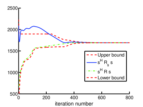
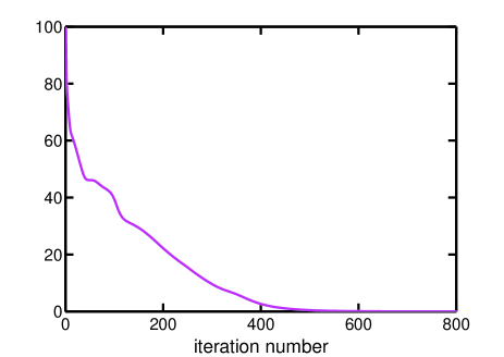
Figure 1: Different metrics versus the iteration number for an UQP solved by MERIT. (a) the UQP objective corresponding to the true matrix (${\boldsymbol{R}}$), the approximated matrix (${\boldsymbol{R}}_{\boldsymbol{s}}$) and also the upper/lower bounds at each iteration. The sub-optimality bounds are updated using (V-C)-(V-C). (b) the criterion $\|{\boldsymbol{E}}\|_{F}=\|{\boldsymbol{R}}-{\boldsymbol{R}}_{s}\|_{F}$ (it reaches values which are practically zero).

Next, we solve the UQP for $20$ full-rank random positive definite matrices of sizes $n\in\{8,16,32,64\}$. Inspired by [11] and [22], we also consider rank-deficient matrices ${\boldsymbol{R}}=\sum_{k=1}^{d}{\boldsymbol{x}}_{k}{\boldsymbol{x}}_{k}^{H}$ where $\{{\boldsymbol{x}}_{k}\}$ are as in (95), but $d\ll n$. The performance of MERIT for different values of $d$ is shown in Table II. Interestingly, the solution of UQP for rank-deficient matrices appears to be obtained more efficiently than for the full-rank matrices. For each problem solved by MERIT, we also let the SDR algorithm of [17] use the same computational time for solving the problem. The SDR algorithm is able to solve the problem only if its core semi-definite program can be solved within the available time. Any remaining time is dedicated to the randomization procedure. The results can be found in Table II. Note that the maximum UQP objective values obtained by MERIT and SDR were nearly identical in those cases in which SDR was able to solve the UQPs in the same amount of time as MERIT. Note also that given the solutions obtained by MERIT and SDR as well as the sub-optimality guarantee of MERIT, a case-dependent sub-optimality guarantee for SDR can be computed as

$$\gamma_{\mbox{SDR}}\triangleq\gamma_{\mbox{MERIT}}\left(\frac{v_{SDR}}{v_{MERIT}}\right).$$ (96)

This can be used to examine the goodness of the solutions obtained by SDR.

$n$	Rank ($d$)	#problems for which $\gamma=1$	Average $\gamma$	Minimum $\gamma$	Average CPU time (sec)	#problems solved by SDR
8	2	$17$	$0.9841$	$0.8184$	$0.13$	$4$
	8	$16$	$0.9912$	$0.9117$	$0.69$	$7$
	2	$15$	$0.9789$	$0.8301$	$1.06$	$2$
16	4	$13$	$0.9773$	$0.8692$	$1.58$	$10$
	16	$4$	$0.9610$	$0.8693$	$3.54$	$13$
	2	$9$	$0.9536$	$0.8190$	$47.04$	$3$
32	6	$4$	$0.9077$	$0.8106$	$55.59$	$7$
	32	$2$	$0.9031$	$0.8021$	$94.90$	$16$
	2	$3$	$0.8893$	$0.8177$	$406.56$	$4$
64	8	$1$	$0.8567$	$0.7727$	$560.35$	$10$
	64	$0$	$0.8369$	$0.7811$	$1017.69$	$15$

TABLE II: Comparison of the performance of MERIT (see Table I) and SDR [17] when solving the UQP for $20$ random positive definite matrices of different sizes $n$ and ranks $d$.

Besides random matrices, we also consider several other matrix structures for which solving the UQP using the proposed method is not “hard”, as explained below.

• Case 1: An exponentially shaped disturbance matrix [1] with correlation coefficient $\eta=0.8$,

  $${\boldsymbol{M}}(k,l)=\eta^{|k-l|},~{}~{}~{}1\leq k,l\leq n.$$ (97)

• Case 2: A disturbance matrix with the structure

  $${\boldsymbol{M}}(k,l)=\eta_{1}^{|k-l|}e^{j2\pi\rho(k-l)}+10\eta_{2}^{|k-l|}+10^{-2}{\boldsymbol{I}}(k,l),~{}~{}~{}1\leq k,l\leq n$$ (98)

  whose terms represent the effects of sea clutter, land clutter and thermal noise, respectively. The values of $(\eta_{1},\eta_{2},\rho)$ are set to $(0.8,0.9,0.2)$ in accordance to an example provided in [23].

• Case 3: A disturbance matrix accounting for both discrete clutter scatterers and thermal noise [17],

  $${\boldsymbol{M}}=\sum_{k=1}^{n_{c}}\eta_{k}{\boldsymbol{p}}_{v_{d,k}}{\boldsymbol{p}}_{v_{d,k}}^{H}+\eta{\boldsymbol{I}}$$ (99)

  where $n_{c}=10$, $\eta_{k}=10^{3}$, $v_{d,k}=(k-1)/2$,

  $${\boldsymbol{p}}_{v_{d,k}}=(1,e^{j2\pi v_{d,k}},\cdots,e^{j2\pi(n-1)v_{d,k}})^{T},~{}~{}~{}1\leq k\leq n_{c},$$ (100)

  and $\eta=10^{-2}$. The chosen values are the same as those considered in [17].

We let ${\boldsymbol{R}}={\boldsymbol{M}}^{-1}\odot({\boldsymbol{p}}{\boldsymbol{p}}^{H})^{*}$ (see (3) and the following discussion) where ${\boldsymbol{p}}$ is an unimodular vector with a structure similar to that of $\{{\boldsymbol{p}}_{v_{d,k}}\}$ in (100). The UQP for the above cases is solved via MERIT using $20$ different random initializations for sizes $n\in\{8,16,32,64\}$. Similar to the previous example, we also used SDR to solve the same UQPs. The results are shown in Table III. The obtained solutions can be considered to be quite accurate in the sense of a sub-optimality guarantee $\gamma$ close to one.

$n$	Rank ($d$)	#problems for which $\gamma=1$	Average $\gamma$	Minimum $\gamma$	Average CPU time (sec)	#problems solved by SDR
	Case 1	$20$	$1.0000$	$1.0000$	$2.82$	$17$
8	Case 2	$20$	$1.0000$	$1.0000$	$0.60$	$20$
	Case 3	$20$	$1.0000$	$1.0000$	$0.27$	$10$
	Case 1	$20$	$1.0000$	$1.0000$	$42.83$	$20$
16	Case 2	$18$	$0.9812$	$0.8075$	$21.58$	$20$
	Case 3	$20$	$1.0000$	$1.0000$	$2.01$	$12$
	Case 1	$20$	$1.0000$	$1.0000$	$990.90$	$20$
32	Case 2	$19$	$0.9995$	$0.9913$	$525.34$	$20$
	Case 3	$20$	$1.0000$	$1.0000$	$7.52$	$7$
	Case 1	$17$	$0.9901$	$0.9862$	$5574.98$	$20$
64	Case 2	$16$	$0.9540$	$0.8359$	$2053.26$	$20$
	Case 3	$20$	$1.0000$	$1.0000$	$22.78$	$9$

TABLE III: Comparison of the performance of MERIT (see Table I) and SDR [17] when solving the UQP for the matrix structures described in Cases 1-3 using $20$ different initializations and for different sizes $n$.

A different code design problem arises when synthesizing waveforms that have good resolution properties in range and Doppler [3]-[5],[24]-[26]. In the following, we consider the design of a thumbtack CAF (see the definitions in sub-section I-A):

$$d(\tau,f)=\left\{\begin{array}[]{ll}n&(\tau,f)=(0,0),\\ 0&\mbox{otherwise.}\end{array}\right.$$ (103)

Suppose $n=53$, let $T$ be the time duration of the total waveform, and let $t_{p}=T/n$ represent the time duration of each sub-pulse. Define the weighting function as

$$w(\tau,f)=\left\{\begin{array}[]{ll}1&(\tau,f)\in\Psi\backslash\Psi_{ml},\\ 0&\mbox{otherwise,}\end{array}\right.$$ (106)

where $\Psi=[-10t_{p},10t_{p}]\times[-2/T,2/T]$ is the region of interest and $\Psi_{ml}=([-t_{p},t_{p}]\backslash\{0\})\times([-1/T,1/T]\\ \backslash\{0\})$ is the mainlobe area which is excluded due to the sharp changes near the origin of $d(\tau,f)$. Note that the time delay $\tau$ and the Doppler frequency $f$ are typically normalized by $T$ and $1/T$, respectively, and as a result the value of $t_{p}$ can be chosen freely without changing the performance of CAF design. The synthesis of the desired CAF is accomplished via the cyclic minimization of (8) with respect to ${\boldsymbol{x}}$ and ${\boldsymbol{y}}$ (see sub-section I-A). In particular, we use MERIT to obtain a unimodular ${\boldsymbol{x}}$ in each iteration. A Björck code is used to initialize both vectors ${\boldsymbol{x}}$ and ${\boldsymbol{y}}$. The Björck code of length $n=p$ (where $p$ is a prime number for which $p\equiv 1~{}(\bmod~{}4)$) is given by ${\boldsymbol{b}}(k)=e^{j(\frac{k}{p})\arccos\left(1/(1+\sqrt{p})\right)}$, $0\leq k<p$, with $(\frac{k}{p})$ denoting the Legendre symbol. Fig. 2 depicts the normalized CAF modulus of the Björck code (i.e. the initial CAF) and the obtained CAF using the UQP formulation in (17) and the proposed method. Despite the fact that designing CAF with a unimodular transmit vector ${\boldsymbol{x}}$ is a rather constrained problem, MERIT is able to efficiently suppress the CAF sidelobes in the region of interest.

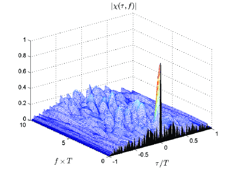
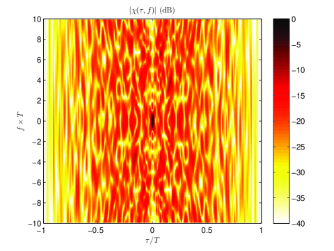
(a) left: 3D plot, right: 2D plot

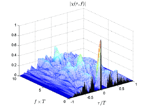
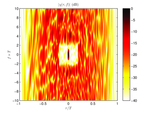
(b) left: 3D plot, right: 2D plot

Figure 2: The normalized CAF modulus for (a) the Björck code of length $n=53$ (i.e. the initial CAF), and (b) the UQP formulation in (17) and MERIT.

VII Concluding Remarks

A computational approach to the NP-hard problem of optimizing a quadratic form over the unimodular vector set (called UQP) has been introduced. The main results can be summarized as follows:

• Some applications of the UQP were reviewed. It was shown that the solution to UQP is not necessarily unique. Several examples were provided for which an accurate global optimum of UQP can be obtained efficiently.

• Using a relaxed version of UQP, a specialized local optimization scheme for UQP was devised and was shown to yield superior results compared to any general local optimization of UQP.

• It was shown that the set of matrices ($\mathcal{K}({\boldsymbol{s}})$) leading to the same solution (${\boldsymbol{s}}$) as the global optimum of UQP is a convex cone. An one-to-one mapping between any two such convex cones was introduced and an approximate characterization of $\mathcal{K}({\boldsymbol{s}})$ was proposed.

• Using the approximate characterization of $\mathcal{K}({\boldsymbol{s}})$, an iterative approach (called MERIT) to the UQP was proposed. It was shown that MERIT provides case-dependent sub-optimality guarantees. The available numerical evidence shows that the sub-optimality guarantees obtained by MERIT are generally better than the currently known approximation guarantee (of $\pi/4$ for SDR).

• Numerical examples were provided to examine the potential of MERIT for different UQPs. In particular, it was shown that the UQP solutions for certain matrices used in active sensing code design can be obtained efficiently via MERIT.

We should note that no theoretical efficiency assessment of the method was provided. It is clear that $\mathcal{C}(V_{\boldsymbol{s}})\cup\mathcal{C}_{\boldsymbol{s}}\subset\mathcal{K}({\boldsymbol{s}})$. A possible approach would be to determine how large is the part of $\mathcal{K}({\boldsymbol{s}})$ that is “covered” by $\mathcal{C}(V_{\boldsymbol{s}})\cup\mathcal{C}_{\boldsymbol{s}}$. However, this problem is left for future work. Furthermore, a study of $m$-UQP using the ideas in this paper will be the subject of another paper.

-A Proof of Theorem 1

In order to verify the first part of the theorem, consider any two matrices ${\boldsymbol{R}}_{1},{\boldsymbol{R}}_{2}\in\mathcal{K}(\widetilde{{\boldsymbol{s}}})$. For any two non-negative scalars $\gamma_{1},\gamma_{2}$ we have that

$${\boldsymbol{s}}^{H}(\gamma_{1}{\boldsymbol{R}}_{1}+\gamma_{2}{\boldsymbol{R}}_{2}){\boldsymbol{s}}=\gamma_{1}{\boldsymbol{s}}^{H}{\boldsymbol{R}}_{1}{\boldsymbol{s}}+\gamma_{2}{\boldsymbol{s}}^{H}{\boldsymbol{R}}_{2}{\boldsymbol{s}}.$$ (107)

Clearly, if some ${\boldsymbol{s}}=\widetilde{{\boldsymbol{s}}}$ is the global maximizer of both ${\boldsymbol{s}}^{H}{\boldsymbol{R}}_{1}{\boldsymbol{s}}$ and ${\boldsymbol{s}}^{H}{\boldsymbol{R}}_{2}{\boldsymbol{s}}$ then it is the global maximizer of ${\boldsymbol{s}}^{H}(\gamma_{1}{\boldsymbol{R}}_{1}+\gamma_{2}{\boldsymbol{R}}_{2}){\boldsymbol{s}}$ which implies $\gamma_{1}{\boldsymbol{R}}_{1}+\gamma_{2}{\boldsymbol{R}}_{2}\in\mathcal{K}(\widetilde{{\boldsymbol{s}}})$.

The second part of the theorem can be shown noting that

$${\boldsymbol{s}}_{2}^{H}({\boldsymbol{R}}\odot({\boldsymbol{s}}_{0}{\boldsymbol{s}}_{0}^{H})){\boldsymbol{s}}_{2} = ({\boldsymbol{s}}_{0}^{*}\odot{\boldsymbol{s}}_{2})^{H}{\boldsymbol{R}}({\boldsymbol{s}}_{0}^{*}\odot{\boldsymbol{s}}_{2})$$

$$= {\boldsymbol{s}}_{1}^{H}{\boldsymbol{R}}{\boldsymbol{s}}_{1}$$

for all ${\boldsymbol{s}}_{1},{\boldsymbol{s}}_{2}\in\Omega^{n}$ and ${\boldsymbol{s}}_{0}={\boldsymbol{s}}_{1}^{*}\odot{\boldsymbol{s}}_{2}$. Therefore, if ${\boldsymbol{R}}\in\mathcal{K}(\widetilde{{\boldsymbol{s}}}_{1})$ then ${\boldsymbol{R}}\odot(\widetilde{{\boldsymbol{s}}}_{0}\widetilde{{\boldsymbol{s}}}_{0}^{H})\in\mathcal{K}(\widetilde{{\boldsymbol{s}}}_{2})$ (for $\widetilde{{\boldsymbol{s}}}_{0}=\widetilde{{\boldsymbol{s}}}_{1}^{*}\odot\widetilde{{\boldsymbol{s}}}_{2}$) and vice versa.

-B Proof of Theorem 2

It is well-known that ${\boldsymbol{x}}^{H}{\boldsymbol{R}}{\boldsymbol{x}}\leq\sigma_{1}\|{\boldsymbol{x}}\|_{2}^{2}$ for all vectors ${\boldsymbol{x}}\in{\mathbb{C}}^{n}$. Let

$${\boldsymbol{\alpha}}^{\prime}=\left(\begin{array}[]{c}{\boldsymbol{\alpha}}\\ {\boldsymbol{0}}_{(n-m)\times 1}\end{array}\right).$$ (111)

It follows from (34) that $\widetilde{{\boldsymbol{s}}}={\boldsymbol{U}}{\boldsymbol{\alpha}}^{\prime}$ and therefore

$$\widetilde{{\boldsymbol{s}}}^{H}{\boldsymbol{R}}\widetilde{{\boldsymbol{s}}} = {\boldsymbol{\alpha}}^{\prime H}{\boldsymbol{\Sigma}}{\boldsymbol{\alpha}}^{\prime}=\sigma_{1}\|{\boldsymbol{\alpha}}^{\prime}\|_{2}^{2}$$

$$= \sigma_{1}\|\widetilde{{\boldsymbol{s}}}\|_{2}^{2}=n\sigma_{1}$$

which implies the global optimality of $\widetilde{{\boldsymbol{s}}}$ for the considered UQP.

-C Proof of Theorem 4

It is worthwhile to observe that the convergence rate of $\{{\boldsymbol{R}}^{(t)}\}$ is not dependent on the problem dimension ($n$), as each entry of $\{{\boldsymbol{R}}^{(t)}\}$ is treated independently from the other entries (i.e. all the operations are element-wise). Therefore, without loss of generality we study the convergence of one entry (say $\{{\boldsymbol{R}}^{(t)}(k,l)\}=\{r_{t}e^{j\theta_{t}}\}$) in the following.

Note that in cases for which $|\theta_{t}-(\phi_{k}-\phi_{l})|>\pi/2$, the next element of the sequence $\{r_{t}e^{j\theta_{t}}\}$ can be written as

$$r_{t+1}e^{j\theta_{t+1}}=r_{t}e^{j\theta_{t}}+\rho e^{j(\phi_{k}-\phi_{l})}$$ (113)

which implies that the proposed operation tends to make $\theta_{t}$ closer to $(\phi_{k}-\phi_{l})$ in each iteration, and finally puts $\theta_{t}$ within the $\pi/2$ distance from $(\phi_{k}-\phi_{l})$.

Let us suppose that $|\theta_{0}-(\phi_{k}-\phi_{l})|>\pi/2$, and that the latter phase criterion remains satisfied for all $\theta_{t}$, $t<T$. We have that

$$r_{T}e^{j\theta_{T}}=r_{0}e^{j\theta_{0}}+T\rho e^{j(\phi_{k}-\phi_{l})}$$ (114)

which yields

$$r_{T}\cos(\theta_{T}-(\phi_{k}-\phi_{l}))=r_{0}\cos(\theta_{0}-(\phi_{k}-\phi_{l}))+T\rho.$$ (115)

Therefore it takes only $T=\left\lceil-r_{0}\cos(\theta_{0}-(\phi_{k}-\phi_{l}))/\rho\right\rceil=1$ iteration for $\theta_{t}$ to stand within the $\pi/2$ distance from $(\phi_{k}-\phi_{l})$.

Now, suppose that $|\theta_{0}-(\phi_{k}-\phi_{l})|\leq\pi/2$. For every $t\geq 1$ we can write that

$$r_{t+1}e^{j\theta_{t+1}} = r_{t}e^{j\theta_{t}}+\rho e^{j(\phi_{k}-\phi_{l})}$$

$$- r_{t}\cos(\theta_{t}-(\phi_{k}-\phi_{l}))e^{j(\phi_{k}-\phi_{l})}$$

$$= e^{j(\phi_{k}-\phi_{l})}\left(\rho+jr_{t}\sin(\theta_{t}-(\phi_{k}-\phi_{l}))\right).$$

Let $\delta_{t+1}=r_{t+1}e^{j\theta_{t+1}}-r_{t}e^{j\theta_{t}}$. The first equality in (-C) implies that

$$\delta_{t+1}=e^{j(\phi_{k}-\phi_{l})}(\rho-r_{t}\cos(\theta_{t}-(\phi_{k}-\phi_{l}))).$$ (117)

On the other hand, the second equality in (-C) implies that

$$\delta_{t+1}=je^{j(\phi_{k}-\phi_{l})}(r_{t}\sin(\theta_{t}-(\phi_{k}-\phi_{l}))~{}~{}~{}~{}~{}~{}~{}~{}~{}~{}~{}~{}$$ (118)

$$-r_{t-1}\sin(\theta_{t-1}-(\phi_{k}-\phi_{l})))$$

for all $t\geq 1$. Note that in (117) and (118), $\delta_{t+1}$ is a complex number having different phases. We conclude

$$\delta_{t+1}=0,~{}~{}\forall~{}t\geq 1$$ (119)

which shows that the sequence $\{r_{t}e^{j\theta_{t}}\}$ is convergent in one iteration. In sum, every entry of the matrix $R$ will converge in at most two iterations (i.e. at most one to achieve a phase value within the $\pi/2$ distance from $(\phi_{k}-\phi_{l})$, and one iteration thereafter).

-D Proof of Theorem 5

We use the same notations as in the proof of Theorem 4. If $|\theta_{0}-(\phi_{k}-\phi_{l})|\leq\pi/2$ then

$$r_{2}e^{j\theta_{2}} = r_{1}e^{j\theta_{1}}$$

$$= r_{0}e^{j\theta_{0}}+\rho e^{j(\phi_{k}-\phi_{l})}$$

$$- r_{0}\cos(\theta_{0}-(\phi_{k}-\phi_{l}))e^{j(\phi_{k}-\phi_{l})}.$$

On the other hand, if $|\theta_{0}-(\phi_{k}-\phi_{l})|>\pi/2$ we have that $r_{1}e^{j\theta_{1}}=r_{0}e^{j\theta_{0}}+\rho e^{j(\phi_{k}-\phi_{l})}$. As a result, $r_{1}\cos(\theta_{1}-(\phi_{k}-\phi_{l}))=\rho+r_{0}\cos(\theta_{0}-(\phi_{k}-\phi_{l}))$ which implies

$$r_{2}e^{j\theta_{2}} = r_{1}e^{j\theta_{1}}+\rho e^{j(\phi_{k}-\phi_{l})}$$

$$- r_{1}\cos(\theta_{1}-(\phi_{k}-\phi_{l}))e^{j(\phi_{k}-\phi_{l})}$$

$$= r_{0}e^{j\theta_{0}}+\rho e^{j(\phi_{k}-\phi_{l})}$$

$$- r_{0}\cos(\theta_{0}-(\phi_{k}-\phi_{l}))e^{j(\phi_{k}-\phi_{l})}.$$

Now, it is easy to verify that (53) follows directly from (-D) and (-D).

-E Proof of Theorem 6

If ${\boldsymbol{s}}$ is a hyper point of UQP associated with ${\boldsymbol{R}}^{(0)}={\boldsymbol{R}}$ then we have that $\arg({\boldsymbol{s}})=\arg({\boldsymbol{R}}{\boldsymbol{s}})$. Let ${\boldsymbol{R}}{\boldsymbol{s}}={\boldsymbol{v}}\odot{\boldsymbol{s}}$ where ${\boldsymbol{v}}$ is a non-negative real-valued vector in ${\mathbb{R}}^{n}$. It follows that

$${\boldsymbol{v}}(k)e^{j\phi_{k}}=\sum_{l=1}^{n}|{\boldsymbol{R}}(k,l)|e^{j\theta_{k,l}}e^{j\phi_{l}}$$ (122)

or equivalently

$${\boldsymbol{v}}(k)=\sum_{l=1}^{n}|{\boldsymbol{R}}(k,l)|e^{j(\theta_{k,l}-(\phi_{k}-\phi_{l}))}$$ (123)

which implies that

$$\left\{\begin{array}[]{l}\sum_{l=1}^{n}|{\boldsymbol{R}}(k,l)|\cos(\theta_{k,l}-(\phi_{k}-\phi_{l}))\geq 0\\ \sum_{l=1}^{n}|{\boldsymbol{R}}(k,l)|\sin(\theta_{k,l}-(\phi_{k}-\phi_{l}))=0\end{array}\right.$$ (126)

for all $1\leq k\leq n$. Now, note that the recursive formula of the sequence $\{{\boldsymbol{R}}^{(t)}\}$ can be rewritten as

$${\boldsymbol{R}}^{(t+1)}={\boldsymbol{R}}^{(t)}-\mathbf{Diag}({\boldsymbol{s}})~{}({\boldsymbol{R}}_{+}^{(t)}-\rho{\boldsymbol{1}}_{n\times n})~{}\mathbf{Diag}({\boldsymbol{s}}^{*})$$ (127)

and as a result,

$${\boldsymbol{R}}^{(t+1)}{\boldsymbol{s}}={\boldsymbol{R}}^{(t)}{\boldsymbol{s}}-\mathbf{Diag}({\boldsymbol{s}})~{}({\boldsymbol{R}}_{+}^{(t)}-\rho{\boldsymbol{1}}_{n\times n})~{}{\boldsymbol{1}}_{n\times 1}.$$ (128)

It follows from (128) that if ${\boldsymbol{s}}$ is a hyper point of the UQP associated with ${\boldsymbol{R}}^{(t)}$ (which implies the existence of non-negative real-valued vector ${\boldsymbol{v}}^{(t)}$ such that ${\boldsymbol{R}}^{(t)}{\boldsymbol{s}}={\boldsymbol{v}}^{(t)}\odot{\boldsymbol{s}}$), then there exists ${\boldsymbol{v}}^{(t+1)}\in{\mathbb{R}}^{n}$ for which ${\boldsymbol{R}}^{(t+1)}{\boldsymbol{s}}={\boldsymbol{v}}^{(t+1)}\odot{\boldsymbol{s}}$ and therefore,

$${\boldsymbol{v}}^{(t+1)}(k)\,e^{j\phi_{k}} = \sum_{l=1}^{n}|{\boldsymbol{R}}^{(t)}(k,l)|e^{j\theta_{k,l}}e^{j\phi_{l}}$$

$$- \left(\left(\sum_{l=1}^{n}{\boldsymbol{R}}^{(t)}_{+}(k,l)\right)-n\rho\right)e^{j\phi_{k}}.$$

Eq. (-E) can be rewritten as

$${\boldsymbol{v}}^{(t+1)}(k) = \sum_{l=1}^{n}|{\boldsymbol{R}}^{(t)}(k,l)|e^{j(\theta_{k,l}-(\phi_{k}-\phi_{l}))}$$

$$- \left(\sum_{l=1}^{n}{\boldsymbol{R}}^{(t)}_{+}(k,l)\right)+n\rho$$

As indicated earlier, ${\boldsymbol{s}}$ being a hyper point for ${\boldsymbol{R}}^{(0)}$ assures that the imaginary part of (-E) is zero. To show that ${\boldsymbol{s}}$ is a hyper point of the UQP associated with ${\boldsymbol{R}}^{(t+1)}$, we only need to verify that ${\boldsymbol{v}}^{(t+1)}(k)\geq 0$:

$${\boldsymbol{v}}^{(t+1)}(k) = \sum_{l=1}^{n}|{\boldsymbol{R}}^{(t)}(k,l)|\cos(\theta_{k,l}-(\phi_{k}-\phi_{l}))$$

$$- \left(\sum_{l=1}^{n}{\boldsymbol{R}}^{(t)}_{+}(k,l)\right)+n\rho$$

$$= n\rho$$

$$+ \sum_{l:~{}(k,l)\notin\Theta}|{\boldsymbol{R}}^{(t)}(k,l)|\cos(\theta_{k,l}-(\phi_{k}-\phi_{l}))$$

Now note that the positivity of ${\boldsymbol{v}}^{(t+1)}(k)$ is concluded from (50). In particular, based on the discussions in the proof of Theorem 4, for $t=1$, there is no $\theta_{k,l}$ such that $|\theta_{k,l}-(\phi_{k}-\phi_{l})|\geq\pi/2$ and therefore ${\boldsymbol{v}}^{(2)}(k)=n\rho$ for all $1\leq k\leq n$. As a result,

$${\boldsymbol{R}}^{(2)}{\boldsymbol{s}}=n\rho{\boldsymbol{s}}$$ (132)

which implies that ${\boldsymbol{s}}$ is an eigenvector of ${\boldsymbol{R}}^{(2)}$ corresponding to the eigenvalue $n\rho$.

References

- [1] A. De Maio, S. De Nicola, Y. Huang, S. Zhang, and A. Farina, “Code design to optimize radar detection performance under accuracy and similarity constraints,” IEEE Transactions on Signal Processing, vol. 56, no. 11, pp. 5618 –5629, Nov. 2008.
- [2] A. De Maio and A. Farina, “Code selection for radar performance optimization,” in Waveform Diversity and Design Conference, Pisa, Italy, June 2007, pp. 219–223.
- [3] H. He, J. Li, and P. Stoica, Waveform Design for Active Sensing Systems: A Computational Approach. Cambridge, UK: Cambridge University Press, 2012.
- [4] N. Levanon and E. Mozeson, Radar Signals. New York: Wiley, 2004.
- [5] H. He, P. Stoica, and J. Li, “On synthesizing cross ambiguity functions,” in IEEE International Conference on Acoustics, Speech and Signal Processing (ICASSP), Prague, Czech Republic, May 2011, pp. 3536–3539.
- [6] J. Li and P. Stoica, Eds., Robust Adaptive Beamforming. NJ, USA.: John Wiley & Sons, Inc., 2005.
- [7] K.-C. Tan, G.-L. Oh, and M. Er, “A study of the uniqueness of steering vectors in array processing,” Signal Processing, vol. 34, no. 3, pp. 245–256, 1993.
- [8] A. Khabbazibasmenj, S. Vorobyov, and A. Hassanien, “Robust adaptive beamforming via estimating steering vector based on semidefinite relaxation,” in Conference on Signals, Systems and Computers (ASILOMAR), California, USA, Nov. 2010, pp. 1102–1106.
- [9] J. Jalden, C. Martin, and B. Ottersten, “Semidefinite programming for detection in linear systems - optimality conditions and space-time decoding,” in IEEE International Conference on Acoustics, Speech, and Signal Processing (ICASSP), vol. 4, Hong Kong, April 2003, pp. 9–12.
- [10] S. Zhang and Y. Huang, “Complex quadratic optimization and semidefinite programming,” SIAM Journal on Optimization, vol. 16, no. 3, pp. 871–890, 2006.
- [11] A. T. Kyrillidis and G. N. Karystinos, “Rank-deficient quadratic-form maximization over M-phase alphabet: Polynomial-complexity solvability and algorithmic developments,” in IEEE International Conference on Acoustics, Speech and Signal Processing (ICASSP), May 2011, pp. 3856–3859.
- [12] S. Verdú, “Computational complexity of optimum multiuser detection,” Algorithmica, vol. 4, pp. 303–312, 1989.
- [13] W.-K. Ma, B.-N. Vo, T. Davidson, and P.-C. Ching, “Blind ML detection of orthogonal space-time block codes: efficient high-performance implementations,” IEEE Transactions on Signal Processing, vol. 54, no. 2, pp. 738–751, feb. 2006.
- [14] T. Cui and C. Tellambura, “Joint channel estimation and data detection for OFDM systems via sphere decoding,” in IEEE Global Telecommunications Conference (GLOBECOM), vol. 6, Texas, USA, Dec. 2004, pp. 3656–3660.
- [15] S. Boyd and L. Vandenberghe, Convex Optimization. Cambridge, UK: Cambridge University Press, 2004.
- [16] M. X. Goemans and D. P. Williamson, “Improved approximation algorithms for maximum cut and satisfiability problems using semidefinite programming,” ACM Journal, vol. 42, no. 6, pp. 1115–1145, Nov. 1995.
- [17] A. De Maio, Y. Huang, M. Piezzo, S. Zhang, and A. Farina, “Design of optimized radar codes with a peak to average power ratio constraint,” IEEE Transactions on Signal Processing, vol. 59, no. 6, pp. 2683–2697, June 2011.
- [18] Z. Q. Luo, W. K. Ma, A.-C. So, Y. Ye, and S. Zhang, “Semidefinite relaxation of quadratic optimization problems,” IEEE Signal Processing Magazine, vol. 27, no. 3, pp. 20 –34, May 2010.
- [19] A. So, J. Zhang, and Y. Ye, “On approximating complex quadratic optimization problems via semidefinite programming relaxations,” Mathematical Programming, vol. 110, pp. 93–110, 2007.
- [20] W. Glunt, T. L. Hayden, and R. Reams, “The nearest doubly stochastic matrix to a real matrix with the same first moment,” Numerical Linear Algebra with Applications, vol. 5, no. 6, pp. 475–482, 1998.
- [21] R. Horn and C. Johnson, Matrix Analysis. Cambridge, UK: Cambridge University Press, 1990.
- [22] G. Karystinos and A. Liavas, “Efficient computation of the binary vector that maximizes a rank-deficient quadratic form,” IEEE Transactions on Information Theory, vol. 56, no. 7, pp. 3581–3593, July 2010.
- [23] A. De Maio, Y. Huang, and M. Piezzo, “A Doppler robust max-min approach to radar code design,” IEEE Transactions on Signal Processing, vol. 58, no. 9, pp. 4943–4947, Sept. 2010.
- [24] P. Stoica, H. He, and J. Li, “New algorithms for designing unimodular sequences with good correlation properties,” IEEE Transactions on Signal Processing, vol. 57, no. 4, pp. 1415–1425, April 2009.
- [25] M. Soltanalian and P. Stoica, “Computational design of sequences with good correlation properties,” IEEE Transactions on Signal Processing, vol. 60, no. 5, pp. 2180–2193, May 2012.
- [26] J. Benedetto, I. Konstantinidis, and M. Rangaswamy, “Phase-coded waveforms and their design,” IEEE Signal Processing Magazine, vol. 26, no. 1, pp. 22–31, Jan. 2009.